Abstract
Empirical-statistical downscaling (ESD) can be a computationally advantageous alternative to dynamical downscaling in representing a high-resolution regional climate. Two distinct strategies of ESD are employed here to reconstruct near-surface winds in a region of rugged terrain. ESD is used to reconstruct the innermost grid of a multiply nested mesoscale model framework for regional climate downscaling. An analog ensemble (AnEn) and a convolutional neural network (CNN) are compared in their ability to represent near-surface winds in the innermost grid in lieu of dynamical downscaling. Downscaling for a 30 year climatology of 10 m April winds is performed for southern MO, USA. Five years of training suffices for producing low mean absolute error and bias for both ESD techniques. However, root-mean-squared error is not significantly reduced by either scheme. In the case of the AnEn, this is due to a minority of cases not producing a satisfactory representation of high-resolution wind, accentuating the root-mean-squared error in spite of a small mean absolute error. Homogeneous comparison shows that the AnEn produces smaller errors than the CNN. Though further tuning may improve results, the ESD techniques considered here show that they can produce a reliable, computationally inexpensive method for reconstructing high-resolution 10 m winds over complex terrain.
1. Introduction
In climate modeling, empirical-statistical downscaling (ESD) is a valuable technique with a prime objective of reliably depicting a region’s climate details not resolved in a relatively coarse-resolution global climate model or in reanalysis data. These regional climate details simultaneously depend on the large-scale weather and climate patterns and also on the local topography and other surface details. In contrast with ESD, dynamical downscaling employs a high-resolution numerical model furnished with initial and boundary conditions from a relatively coarse-resolution prediction or reanalysis to directly simulate smaller-scale details of a region’s climate. The latter approach is usually preferred when seeking the most accurate representation of the fine-scale atmospheric state of a region. However, ESD can be a computationally attractive alternative to dynamical downscaling when dealing with climate timescales and large regional climate datasets.
The essential objective of ESD is to establish empirical relationships from historical data between large-scale atmospheric conditions and local-scale weather and climate patterns. The majority of ESD approaches fall into three categories: regression-based techniques, weather classification approaches, and stochastic weather generators [1]. Regression-based techniques and weather classification methods are the primary emphasis of this study, so the reader is referred to [1] for further information on the weather generator technique.
Regression-based ESD varies widely in complexity from multilinear regression [2] and generalized learning models [3] to machine learning and artificial intelligence models [4,5,6]. Regression techniques establish either linear or nonlinear relationships between a set of predictors and a predictand. The typical application of regression-based ESD is spatial downscaling.
One of the primary weather classification approaches is the analog-based methods of ESD. The inception of analog techniques dates back to Lorenz’s [7] paper on using historical analog weather patterns to predict future weather. A fundamental challenge of the analog technique, however, is that a best matching historical event will not evolve in exactly the same way as the current pattern. This challenge is typically overcome by constructing an ensemble of best matching historical events and combining them in a way that optimally reproduces the target pattern [8,9,10,11,12,13]. Limitations to analog methods include the following: the requirement of a large historical record of observations to adequately identify an analog atmospheric state, simulated predictands cannot be found if they occur outside the range of historical analogs, and the method may suffer in the case of a non-stationary baseline climate [8,14,15,16].
While there are now many applications of downscaling in the geosciences at numerous timescales, ranging from weather to climate applications, a relatively novel area for downscaling applications is in deriving from climatology typical regional mesoscale flow patterns in the planetary boundary layer (PBL). One example is a climatological-based typical-day dispersion pattern for hazardous releases of a given tracer field [17]. Another area concerned with PBL flow patterns is in quantifying a region’s wind power capabilities from regional climate characteristics [18]. Moreover, while ESD techniques typically use both historical model data and observations to downscale climate variables from a global circulation model to a regional scale, ESD can be used simply as an alternative to high-resolution inner nests in dynamical models to reconstruct regional climate variables.
In this paper, two ESD downscaling strategies are applied to reconstruct climatological 10 m wind speeds in lieu of high-resolution dynamical downscaling in a region with complex terrain. The first method is a simple analog method known as the analog ensemble [10], and the second method is a regression-based technique that is the convolutional neural network. These two ESD schemes were also used in [19] but for downscaling precipitation in complex topography instead of 10 m winds. It will be shown that both techniques perform well in producing a low mean absolute error, but some outlier cases contribute to a higher root-mean-squared error.
2. Methods
The overall purpose of this work was to demonstrate and compare two types of ESD techniques for PBL parameters. The focus of the present study was on reconstructing 10 m winds. It should be noted, however, that the methods of this work can be generalized to other PBL parameters in a straightforward manner. The two ESD techniques demonstrated here are the analog ensemble and the convolutional neural network methods. A mesoscale model with nested grids was used to perform high-resolution dynamical downscaling over a domain of interest, which provided the two ESD techniques with sufficient training and testing data. These ESD techniques were applied to the innermost grid nest to achieve a computationally inexpensive high-resolution reconstruction of near-surface winds over a climate timescale.
Dynamical downscaling was performed using the Weather Research and Forecasting (WRF) model [20]. The WRF model version applied here was 3.5.1, and the WRF was run using the Global Climatology Analysis Tool (GCAT) [17]. In particular, GCAT was used here to produce a regional 30 year climatology of PBL parameters over the years 1988–2017 and for a period of 1 month (0000 UTC 1 April–2300 UTC 30 April). Each year’s initialization and lateral boundary conditions, the latter of which are available in 6 h increments, came from the NOAA Climate Forecast System Reanalysis (CSFR) dataset and were nudged toward the Global Data Assimilation System (GDAS) observations. The WRF was run with four 66 × 66 grids centered at 36.8° N and 91.39° W (Figure 1) to downscale the CSFR 0.5 °C dataset on the nested grids containing 30, 10, 3.3, and 1.1 km grid spacings. The model configuration also included 56 vertical levels extending up to 50 hPa. The center of the innermost high-resolution grid (grid 4) was in southern Missouri USA. The WRF model was restarted every 5 days at 0000 UTC. The physics parameterizations included WRF single-moment microphysics, Kain–Fritsch cumulus parameterization on grids 1 and 2, the rapid radiative transfer model (RRTM) with Dudhia long- and short-wave radiation schemes, the Yonsei University (YSU) PBL scheme, and the Noah land-surface model.
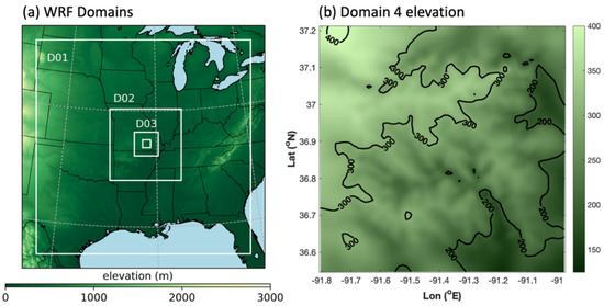
Figure 1.
(a) A geographic representation of the four nested WRF domains used in this study with surface elevation (m) above sea level shown in green shading; (b) a more detailed presentation of the surface elevation above sea level (m) in the innermost grid (i.e., grid 4).
Two post-processing techniques were used to statistically downscale WRF grid 3 (the penultimate nest at 3.3 km grid spacing) and grid 4. As mentioned previously, the two schemes demonstrated here are the analog ensemble (AnEn) and the convolutional neural network (CNN). The AnEn is a weather classification technique, and the CNN is a nonlinear regression, machine learning technique. The details of each method are summarized below.
The AnEn algorithm was initially developed in [10] for the ensemble prediction of PBL parameters. More recently, the AnEn was successfully applied in downscaling precipitation [19,21]. In the current application, the AnEn was used to downscale 10 m winds from the 3.3 km WRF grid 3 to the 1.1 km grid 4. The most fundamental goal was to produce a representation of high-resolution winds that was more accurate than simply interpolating grid 3 10 m winds to grid 4. To this end, the 30 years of WRF April simulations covering 1988–2017 were divided into training and testing groups, with 2013–2017 arbitrarily chosen as training data and 1988–2012 serving as testing and evaluation data. In both the training and testing groups, certain PBL-related fields from grid 3 were interpolated to grid 4 to compare against the dynamically downscaled grid 4. The particular fields considered in this study included the 10 m components of the horizontal wind (u and v), mean sea-level pressure (ps), the Monin–Obukhov length (L), and the PBL height (HPBL). These interpolated data were used as AnEn predictors to determine the downscaled u and v at each grid point in grid 4.
The details of the AnEn downscaling methodology are described as follows. For each grid point on grid 4, the AnEn was run to downscale for grid 4 u and v using grid 3 data. At each grid point, the interpolated u, v, ps, L, and HPBL were used as AnEn features (also known as predictors in prediction applications). The AnEn downscaling strategy for each grid point is sketched out in Figure 2. When evaluating the testing data for each hour and grid point on grid 4, there were 5 years of hourly training data covering a certain time period (e.g., a month). In other words, for reconstructing high-resolution winds in the month of April, there were 5 years × 24 h × 30 days = 3600 hourly training cases per grid point (for the period between 2013 and 2017). By similar reasoning, there were 18,000 hourly testing cases per grid point (for April data between 1988 and 2012). Similar to the case in [22], AnEn predictor weighting was optimized individually for each grid point. Optimal weighting as determined from finding weights that minimize bias in the training data is shown in Figure 3. It is worth noting that this was done using brute force and may not be practical to do in a real-time setting, but there are more efficient forward selection features [23]. The downscaled value for u and v was the mean of 20 ensemble members. Twenty members and the simple mean were chosen since they performed the best in trial-and-error testing. While not considered in the current study, a neighborhood averaging method for downscaling at each grid point as described in [11] may be a way to further improve this method.
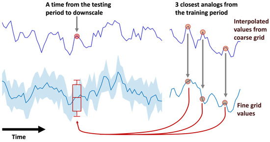
Figure 2.
A conceptual diagram of the AnEn method applied to a given grid point and time in the testing period. The top curve shows a timeseries of a particular variable (i.e., u, v, ps, L, or HPBL) interpolated from the coarse grid to the fine grid, with the left-hand timeseries representing the testing period and the right-hand series representing the training period. The bottom curve and ensemble spread at the left is constructed from the AnEn estimates of the dynamically downscaled variable whereas the bottom right curve is the actual WRF downscaled variable. In this example, three analogs to the given grid point and time are found in the training period using the five AnEn variables (or “predictors”) u, v, ps, L, and HPBL. Furthermore, real-world applications of the AnEn typically have many more ensemble members (20 are used in this study). The three-member ensemble shown here, then, provides a range of values of the empirically downscaled variable (u and v in the current application). The mean is used in this situation for the downscaled u and v values. This figure was adapted from Figure 1 in [24].
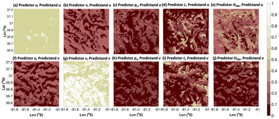
Figure 3.
The spatial distribution of variable weighting. The top row (a–e) here shows the weighting for variables (predictors) u, v, ps, L, and HPBL, respectively, chosen for downscaling u. The bottom row (f–j) is the same as the top row except for downscaling v. The weights in each row add up to 1 at every grid point.
As an alternative regression-based method to the weather-classification AnEn method, a convolutional neural network (CNN) was applied to the entire grid 3 and grid 4 fields to empirically reconstruct u and v from grid 3 to grid 4. CNNs are a type of artificial neural network that are applied to imagery to discern nonlinear relationships between input data and a predictand. The derivation of a CNN entails training a kernel weighting matrix that is passed over an image to abstract relevant image features. This process can be continued over a number of times (layers). Weights are found iteratively through backward optimization and gradient descent. In particular, each iteration is performed to minimize the cost of a loss function, which is the mean-squared error between the CNN output and the target post-processed variable. In each iteration, the gradient field of the weights with respect to the loss function is calculated and a step is taken in the opposite direction of the gradient.
In a similar vein to [19], the CNN in the current application used multiple PBL fields to reconstruct u and v from the 66 × 66–sized grid 3 to the higher-resolution 66 × 66–sized grid 4. The PBL fields input into the CNN were the same five u, v, ps, L, HPBL variables used in the AnEn method. As before, the downscaling application was conducted in the month of April. Per sample, the input data formed a 66 × 66 × 5 variable matrix, which provided a spatial relationship that the convolutional kernels learned. After two convolutional layers, the resulting salient feature maps were flattened and used as input in a feed-forward neural network producing downscaled u or v fields on the high-resolution 66 × 66–sized grid 4. It is worth emphasizing that CNNs are derived individually for downscaling u and v. The actual downscaled WRF variables on grid 4 were used to establish the mean-squared error (MSE) that served as the loss function. To train the CNN, the years 1988–1992 were used. Years 1996–2017 were used as validation in the training process. The CNN was tested on years 1993–1995. To later compare with the AnEn, the AnEn was retrained on data from the years 1988–1992 and tested on the years 1993–1995 in order to ensure a homogeneous comparison. The CNN architecture parameters are summarized in Table 1 and were guided by Meech et al.’s [19] successful application of the CNN to downscaling. Considerable trial and error runs were performed on the CNN architecture parameters to seek optimal performance, but the configuration in [19] worked best. The Python library Keras [25] with a TensorFlow Backend [26] was used to train the CNN.

Table 1.
The architecture of the CNN used to reconstruct both u and v. Input is 66 × 66 grid points and five input forecast fields (u, v, ps, L, and HPBL). Leaky ReLU activation is used in every layer except in the final layer, which is activated through a linear function for the final downscaled field. The loss is defined as the mean-squared error (MSE) between the output and actual grid 4 WRF downscaled variable.
To ensure a reduced computational cost in using the AnEn or CNN for a 30 year regional climatology of high-resolution winds, this study chiefly considered the scenario where 5 years of training data were generated by the high-resolution configuration of WRF (i.e., with four grids) and where 25 years of data were generated using the coarser-resolution configuration of WRF (i.e., with three grids). In practice, spatially constant predictor weighting in the case of the AnEn and a fixed architecture (i.e., set number of convolutional layers) of the CNN can be imposed without any major impact on the quality of the reconstructed 10 m grid 4 winds. In these scenarios, the computational cost savings of using either ESD scheme to reconstruct 25 years of grid 4 10 m winds resulted in a roughly 10 times faster execution than that of running the full-resolution WRF for all 30 years.
3. Results
3.1. The Analog Ensemble
As stated earlier, 20 analog ensemble members were averaged at each grid point on grid 4 to reconstruct u and v from grid 3 with the AnEn ESD method. The performance of the AnEn was examined here with basic statistics, including spatial mean absolute error (MAE), spatial bias, and spatial root-mean-squared error (RMSE). These error metrics were computed for the testing period (1988–2012) by comparing the AnEn and interpolated fields to the dynamically downscaled result for grid 4. This evaluation included all 30 days of April at each hour of day.
Figure 4 shows the MAE on grid 4 associated with both simple interpolation and the AnEn reconstruction of 10- m winds. It is immediately clear that the AnEn performs better than interpolation in terms of MAE for both the u and v components of 10-m wind. The area-averaged MAE for u improved from 0.052 to 0.019 m s−1 when using the AnEn instead of interpolation. The improvement in MAE for v was from 0.066 to 0.010 m s−1. Both the interpolated and AnEn error spatial distributions seen in Figure 4 are noisy. It is possible that this cellular error pattern was related to complex terrain effects on low-level flow, but further investigation would be required to confirm this.
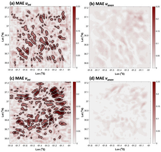
Figure 4.
The grid 4 spatial distribution of MAE for (a) interpolated u (domain average MAEave = 0.052 m s−1), (b) the AnEn-produced u (MAEave = 0.019 m s−1), (c) interpolated v (MAEave = 0.066 m s−1), and (d) AnEn-produced v (MAEave = 0.010 m s−1). Here, solid contours are plotted every 0.1 m s−1.
Another vital error metric is the bias, which is closely related to MAE in that it is the same metric but without an absolute value applied to each term in the summation of errors across the entire sample. Unlike MAE, the area-averaged AnEn bias did not appear to be superior to that of simple interpolation. In fact, there was a negative bias of −0.019 and −0.007 m s−1 for the AnEn downscaled u and v. Compared to the area-average biases for interpolated u and v (0.004 and 0.006 m s−1), the AnEn was mildly worse. However, the spatial distributions of bias tell a significantly different story. Figure 5 shows that interpolated fields of bias have relatively high-amplitude regions of negative and positive bias (with magnitudes of about 0.25 m s−1). The area-average of bias happened to obscure localized peaks in the bias for the interpolated results. This mirage is unveiled in the MAE panels of Figure 4a,c, which reveal that the area-average leads to the cancelation of oppositely signed regions of enhanced error. On the other hand, the AnEn produced comparatively less noisy bias fields, indicating that its small overall area-average bias was representative of most grid points. The MAE confirmed this result.
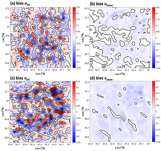
Figure 5.
The grid 4 spatial distribution of bias for (a) interpolated u (domain average biasave = 0.004 m s−1), (b) the AnEn-produced u (biasave = −0.019 m s−1), (c) interpolated v (biasave = 0.006 m s−1), and (d) AnEn-produced v (biasave = −0.007 m s−1). Here, solid contours are plotted every 0.1 m s−1, with negative contours plotted at the same interval indicated by dotted lines.
At first glance, the RMSE results for the AnEn were not as successful as the MAE and bias results (Figure 6). The RMSE domain averages and overall spatial distribution of errors were similar for both interpolation and the AnEn. However, the peak magnitudes of RMSE were not as high in the AnEn RMSE fields as in the interpolated fields. Therefore, the spatial peaks in RMSE-type errors were reduced by the AnEn, which implies that RMSE errors must have been a bit worse in other regions to obtain its area-average result. This was confirmed in a cumulative distribution function of domain-average wind speed RMSE shown in Figure 7. Here, the RMSE was sorted from best to worst for both the AnEn and interpolation for all 18,000 cases in the testing dataset. The best performing AnEn cases did not produce RMSE as low as the best performing interpolation cases, but for the majority of cases where interpolation produced worse errors (RMSE > 0.31 m s−1), the AnEn performed better. Shown in Figure 7b is a scatter diagram of the RMSEs for the AnEn versus interpolation. The scatterplot emphasizes that, more often than not, the AnEn reduced the error, but there is a wide range of scatter above the one-to-one diagonal, showing that the AnEn’s overall RMSE was being penalized by a relative minority of cases.
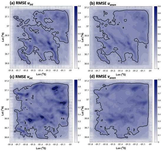
Figure 6.
The grid 4 spatial distribution of RMSE for (a) interpolated u (domain average RMSEave = 0.347 m s−1), (b) the AnEn-produced u (RMSEave = 0.371 m s−1), (c) interpolated v (RMSEave = 0.399 m s−1), and (d) AnEn-produced v (RMSEave = 0.398 m s−1). Here, solid contours are plotted every 0.3 m s−1, with negative contours plotted at the same interval indicated by dotted lines.
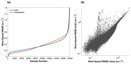
Figure 7.
(a) Cumulative distribution functions of the RMSE for the wind speed associated with the AnEn (blue) and interpolation (red); (b) A scatterplot of RMSE for the AnEn versus interpolation. A logarithmic scale for the axes in (b) was chosen to emphasize the majority of points concentrated at RMSEs less than 1 m s−1.
An inspection of the case studies showed that the majority of AnEn reconstructed wind fields scrupulously reproduced the fine-scale details of WRF grid 4 wind speed patterns when compared against a smoothed-out interpolated field. However, as can be discerned in Figure 7b, there were a minority of instances where the downscaled AnEn field did not faithfully reproduce the verifying WRF solution for grid 4. Figure 8 shows a typical example of one of the poorly behaved AnEn cases for total wind speed (RMSE = 1.6 m s−1) for 0400 UTC 23 April 2006. Here, the AnEn structurally resembled the interpolated field more than the WRF field. In fact, the interpolated field better resolved some of the higher-amplitude winds. However, the majority of case studies were consistent with the results of Figure 7, showing that the AnEn better resembled the WRF’s dynamically downscaled fields for grid 4. A typical example is shown in Figure 9 for 1200 UTC 1 April 1988. The AnEn was able to better resolve small-scale details that were not resolved by interpolation from grid 3. Nonetheless, future research should be conducted to more closely investigate the few pathological cases in order to understand why the empirical downscaling technique does not work well in some cases. One hypothesis is that the testing sample contains weather patterns that are not well captured in the training data. Indeed, a sensitivity experiment (not shown) using 15 years of training data greatly reduces all types of AnEn errors, including the RMSE.
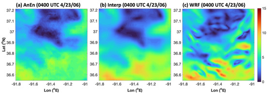
Figure 8.
An example of a poor AnEn reconstruction of grid 4 winds for the total wind speed (RMSE = 1.6 m s−1). Plotted here is the grid 4 wind speed (m s−1) at 0400 UTC 23 April 2006 produced by (a) the AnEn, (b) the interpolation, and (c) the WRF.
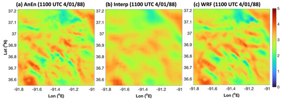
Figure 9.
An example of a typical AnEn reconstruction of the total wind speed (RMSE = 0.2 m s−1). Plotted here is the grid 4 wind speed (m s−1) at 1100 UTC 1 April 1988 produced by (a) the AnEn, (b) the interpolation, and (c) the WRF.
3.2. The Convolutional Neural Network
The evaluation of the CNN ESD method for reconstructing high-resolution winds was done in exactly the same manner as in the AnEn error analysis above. For example, Figure 10 shows the fields of MAE for the 10-m u and v wind components downscaled from grid 3 to grid 4 through simple interpolation and with the CNN. Qualitatively, the MAE results were similar to the AnEn versus interpolation results. The CNN improved area-averaged MAE, though the fractional improvement was not as great as that for the AnEn. However, it is important to note that the AnEn was tested for many more years than the three (1993–1995) used in the evaluation of the CNN. To more rigorously compare the AnEn and CNN, a homogeneous comparison of the two ESD techniques follows in Section 3.3.
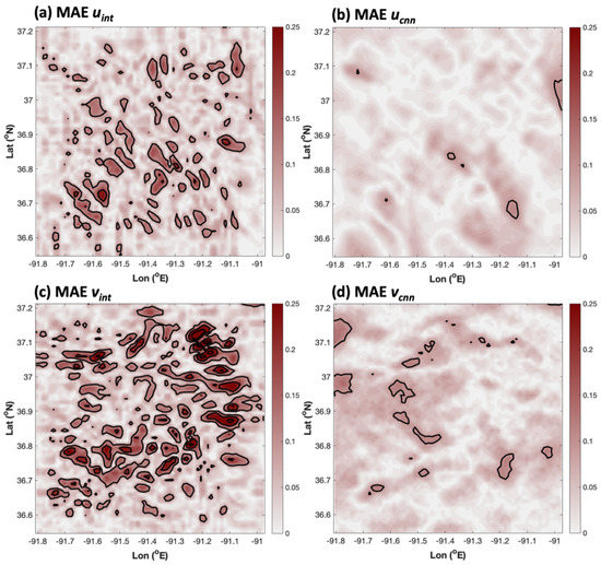
Figure 10.
The grid 4 spatial distribution of MAE for (a) interpolated u (domain average MAEave = 0.050 m s−1), (b) the CNN-produced u (MAEave = 0.029 m s−1), (c) interpolated v (MAEave = 0.068 m s−1), and (d) CNN-produced v (MAEave = 0.041 m s−1). Here, solid contours are plotted every 0.1 m s−1.
Figure 11 depicts the spatial distributions of bias for both the interpolated and CNN-reconstructed u and v fields. Once again, the spatial distribution of error for the CNN was better than that obtained by simply interpolating data from grid 3 to grid 4, though the relative improvements were not as great as seen in the case of the AnEn. Offsetting biases are an issue for both the interpolation and CNN results, so area averages are deceptive when comparing performance, though once again the interpolated fields and offsetting bias errors across the domain yielded smaller area-averaged bias magnitudes for both u and v.
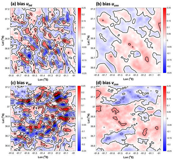
Figure 11.
The grid 4 spatial distribution of bias for (a) interpolated u (domain average biasave = 0.002 m s−1), (b) the CNN-produced u (biasave = 0.012 m s−1), (c) interpolated v (biasave = 0.009 m s−1), and (d) CNN-produced v (biasave = 0.017 m s−1). Here, solid contours are plotted every 0.1 m s−1, with negative contours plotted at the same interval indicated by dotted lines.
Finally, the RMSE for the CNN versus interpolation is displayed in Figure 12. As in the case of the AnEn, RMSE was not improved with CNN-based downscaling. In fact, in the case of the CNN, the RMSE was actually qualitatively worse than that resulting from interpolation for both u and v. However, simple interpolation does result in some isolated regions of enhanced RMSE exceeding the maxima in CNN-based RMSE.
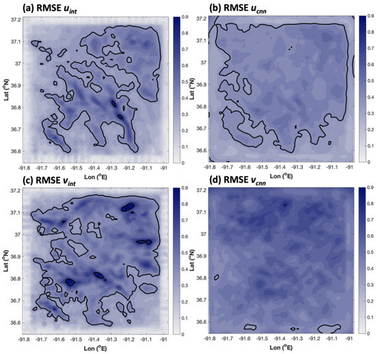
Figure 12.
The grid 4 spatial distribution of RMSE for (a) interpolated u (domain average RMSEave = 0.333 m s−1), (b) the CNN-produced u (RMSEave = 0.414 m s−1), (c) interpolated v (RMSEave = 0.380 m s−1), and (d) CNN-produced v (RMSEave = 0.553 m s−1). Here, solid contours are plotted every 0.3 m s−1, with negative contours plotted at the same interval indicated by dotted lines.
Figure 13 shows a typical case study of CNN-based ESD for reconstructing high-resolution wind speed. This specific example was for 1400 UTC 2 April 1993. When comparing with the elevation data in Figure 1, it becomes evident that the higher wind speeds occurred on ridges, giving the wind speed its conspicuous tendril-like structure. Similar to the AnEn case studies, the CNN-based ESD method produced a more fine-scale wind structure on grid 4 than did the simple interpolation of grid 3 data to grid 4. In this example, the fine-scale details qualitatively agreed with the verifying dynamically downscaled winds produced by WRF. However, the CNN did not quite capture the highest and lowest values of wind speed in the domain, contributing to some of the nonzero RMSE values. Systematically, these types of case-by-case amplitude errors sum up to the elevated RMSE errors seen in Figure 12.
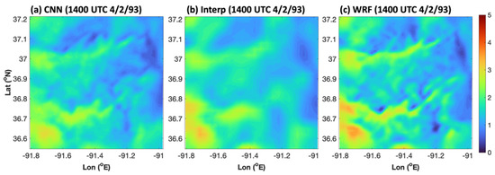
Figure 13.
An example of a typical CNN downscaling for the total wind speed (RMSE = 0.24 m s−1). Plotted here is the grid 4 wind speed (m s−1) at 1400 UTC 2 April 1993 produced by (a) the CNN, (b) the interpolation, and (c) the WRF.
3.3. A Homogeneous Comparison of the AnEn and the CNN
To fairly evaluate the relative performance of the AnEn versus the CNN ESD methods, it is necessary that the two techniques are trained and tested on the exact same data samples. To achieve this, both the AnEn and CNN were trained over the 1988–1992 time period. Here, the weighting scheme devised in Figure 3 was used for the AnEn. The AnEn was then tested over the 1993–1995 time period as in the CNN evaluation. This was a strict evaluation of the AnEn in that the CNN used data from 1996 to 2017 for validation purposes in training the CNN, whereas the AnEn did not enjoy this advantage. On the other hand, it is possible that the subjective and clearly imperfect process of trial and error did not optimize the CNN, so general conclusions drawn from this comparison should still be treated with some caution.
Figure 14 shows the difference fields in MAE and RMSE for the AnEn versus the CNN as determined through homogeneous comparison. In this case, any positive region would indicate that the AnEn produced higher errors, and any negative region would indicate that the CNN produced worse errors. The differences in MAE in Figure 14a,b visually look like a competitive draw between the two schemes in reconstructing the high-resolution u and v, but a domain average shows that the CNN produced about 0.010 m s−1 higher values of MAE overall for u. In the case of v, the AnEn’s relative performance in terms of MAE was even better, with the area-average difference being twice as large as in the case of u. More substantial differences appeared in the RMSE difference fields (Figure 14c,d), especially in the case of the v field. Here, it was quite apparent that the RMSE error increased away from the center in the CNN results relative to the AnEn results. This spatial pattern is consistent with the individual RMSE results for the AnEn and CNN summarized in Section 3.1 and Section 3.2.
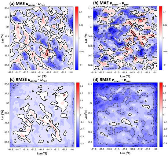
Figure 14.
The grid 4 spatial distribution of differences in MAE between the AnEn and CNN for (a) u (domain average DMAEave = −0.010 m s−1) and (b) v (DMAEave = −0.019 m s−1) and grid 4 spatial distributions of differences in RMSE between the AnEn and CNN for (c) u (DRMSEave = −0.035 m s−1) and (d) v (DRMSEave = −0.162 m s−1). In (a,b), solid contours are plotted every 0.05 m s−1, with negative contours at the same intervals indicated by dotted lines. In (c,d), solid contours are plotted every 0.15 m s−1, with negative contours at the same intervals indicated by dotted lines.
4. Discussion and Conclusions
In this study, two distinct strategies for empirical-statistical downscaling (ESD) of near-surface winds in a region containing rugged terrain were compared. The motivation for ESD was derived from the fact that high-resolution dynamical downscaling with a numerical mesoscale model often involves a series of nested grids, with the innermost grid containing the smallest spatial grid spacing. ESD was proposed in this context as a computationally inexpensive alternative to dynamical downscaling for reconstructing high-resolution fields of 10 m winds in the innermost grid, with the potential to generalize to ESD over multiple nests. To perform ESD on the innermost grid, an analog ensemble (AnEn) was used as a weather classification ESD approach and a convolutional neural network (CNN) was employed as a regression-based ESD option. In the current downscaling setting, a 30 year climatology of hourly 10 m wind was considered for southern MO, USA, over the month of April. The methods demonstrated here are readily extensible to other variables, regions, and time periods.
The 30 year climatology of 10 m wind in this study covers the years from 1988 to 2017. This 30 year time period was divided into training and testing periods for the AnEn and CNN. Using 5 years of training was sufficient to produce low mean absolute error and bias for both ESD approaches. An ESD method that can reconstruct climatological depictions of high-resolution 10 m winds as a computationally inexpensive alternative to high-resolution dynamical downscaling and do so with low bias would be beneficial in a number of applications, including studies involving wind power generation potential. In contrast with the low bias and mean absolute error, the root-mean-squared error was not significantly reduced by either ESD scheme, especially in the case of the CNN. For the AnEn, this undesirable result was shown to be a consequence of a minority of cases not producing a reliable reconstruction of low-level winds, which augmented the root-mean-squared error while keeping the mean absolute error small. The CNN, on the other hand, often underestimated the wind speed extrema in the grid 4 domain. Using a direct homogeneous comparison, the AnEn produced smaller errors than the CNN. This does not necessarily imply that one technique is fundamentally superior to the other because the hyperparameters and architecture design of the CNN span a capacious space that is impractical to explore fully by trial and error. By the same token, the AnEn can likely be further improved by including additional variables, changing the training strategy, or considering a neighborhood approach similar to that produced in [11]. Nonetheless, the results here show the existence of two distinct ESD techniques that offer a computationally inexpensive alternative to high-resolution dynamical downscaling for 10 m wind over rugged terrain with mean absolute errors that are significantly lower than those for simple interpolation.
Author Contributions
Conceptualization, S.A; methodology, S.A. and C.M.R.; software, S.A. and C.M.R.; validation, C.M.R.; formal analysis, C.M.R.; writing—original draft preparation, C.M.R. and S.A.; funding acquisition, S.A. All authors have read and agreed to the published version of the manuscript.
Funding
The National Center of Atmospheric Research is sponsored by the National Science Foundation.
Institutional Review Board Statement
Not applicable.
Informed Consent Statement
Not applicable.
Data Availability Statement
Anyone interested in data involved with this research may contact the corresponding author for full access to data.
Acknowledgments
We would like to thank the National Ground Intelligence Center (NGIC) of the U.S. Army for supporting the development of the Global Climatological Analysis Tool (GCAT). This material is also based upon work supported by the National Center for Atmospheric Research, which is a major facility sponsored by the National Science Foundation under Cooperative Agreement no. 1852977. Furthermore, we are grateful for the patient help of Howard Soh, Rong Shyang Sheu, and Francois Vandenberghe (NCAR) for help with running the GCAT system. Will Chapman (NCAR) kindly provided the initial CNN Python scripts that were used and modified in this manuscript and also provided helpful advice in the early stages of training the model. Xiaodong Chen (NWRA)’s GitHub-provided Python routine was used to plot the WRF domains in Figure 1a. We thank two anonymous reviewers for comments that helped improve this manuscript.
Conflicts of Interest
The authors declare no conflict of interest. The funders had no role in the design of the study; in the collection, analyses, or interpretation of data; in the writing of the manuscript; or in the decision to publish the results.
References
- Wilby, R.L.; Charles, S.P.; Zorita, E.; Timbal, B.; Whetton, P.; Mearns, L.O. Guidelines for use of climate scenarios developed from statistical downscaling methods. In Supporting Material of the Intergovernmental Panel on Climate Change; World Meteorological organization: Geneva, Switzerland, 2004; pp. 3–21. [Google Scholar]
- Sachindra, D.A.; Huang, F.; Barton, A.F.; Perera, B.J.C. Multi-model ensemble approach for statistically downscaling general circulation model output to precipitation. Q. J. R. Meteorol. Soc. 2014, 140, 1161–1178. [Google Scholar] [CrossRef] [Green Version]
- Beecham, S.; Rashid, M.; Chowdhury, R.K. Statistical downscaling of multi-site daily rainfall in a south Australian catchment using a generalized linear model. Int. J. Climatol. 2014, 34, 3654–3670. [Google Scholar] [CrossRef]
- Tripathi, S.; Srinivas, V.V.; Nanjundiah, R.S. Downscaling of precipitation for climate change scenarios: A support vector machine approach. J. Hydrol. 2006, 330, 621–640. [Google Scholar] [CrossRef]
- Sachindra, D.A.; Ahmed, K.; Rashid, M.M.; Shahid, S.; Perera, B.J.C. Statistical downscaling of precipitation using machine learning techniques. Atmos. Res. 2018, 212, 240–258. [Google Scholar] [CrossRef]
- Hsu, K.; Sorooshian, S.; Pan, B.; Aghakouchak, A. Improving precipitation estimation using convolutional neural network. Water Resour. Res. 2019, 55, 2301–2321. [Google Scholar]
- Lorenz, E.N. Atmospheric predictability as revealed by naturally occurring analogues. J. Atmos. Sci. 1969, 26, 636–646. [Google Scholar] [CrossRef] [Green Version]
- Zorita, E.; von Storch, H. The analog method as a simple statistical downscaling technique: Comparison with more complicated methods. J. Clim. 1999, 12, 2474–2489. [Google Scholar] [CrossRef]
- Hidalgo, H.G.; Dettinger, M.D.; Cayan, D.R. Downscaling with constructed analogues: Daily precipitation and temperature fields over the United States. In CEC PIER Project Report CEC-500-2007-123; California Energy Commission: Sacramento, CA, USA, 2008; 48p. [Google Scholar]
- Monache, L.D.; Eckel, F.A.; Rife, D.L.; Nagarajan, B.; Searight, K. Probabilistic weather prediction with an analog ensemble. Mon. Weather Rev. 2013, 141, 3498–3516. [Google Scholar] [CrossRef] [Green Version]
- Pierce, D.W.; Cayan, D.R.; Thrasher, B.L. Statistical downscaling using Localized Constructed Analogs (LOCA). J. Hydrometeorol. 2014, 15, 2558–2585. [Google Scholar] [CrossRef]
- Bettoli, M.L. Analog Methods for Empirical-Statistical Downscaling. Oxford Research Encyclopedia of Climate Science. 2021. Available online: https://oxfordre.com/climatescience/view/10.1093/acrefore/9780190228620.001.0001/acrefore-9780190228620-e-738 (accessed on 31 January 2022).
- Ghilain, N.; Vannitsem, S.; Dalaiden, Q.; Goosse, H.; De Cruz, L.; Wei, W. Reconstruction of daily snowfall accumulation of 5.5 km resolution over Dronning Maud Land, Antarctica, from 1850 to 2014 using an analog-based downscaling technique. Earth Syst. Sci. Data Discuss 2021. [Google Scholar] [CrossRef]
- Benestad, R.E. Downscaling precipitation extremes: Correction of analog methods through PDF predictions. Theor. Appl. Climatol. 2010, 100, 1–21. [Google Scholar] [CrossRef] [Green Version]
- Gutiérrez, J.M.; San Martin, D.; Brands, S.; Manzanas, R.; Herrera, S. Reassessing statistical downscaling techniques for their robust application under climate change conditions. J. Clim. 2013, 26, 171–188. [Google Scholar] [CrossRef] [Green Version]
- Castellano, C.M.; De Gaetano, A.T. Downscaling extreme precipitation from CMIP5 simulations using historical analogs. J. Appl. Meteorol. Climatol. 2017, 56, 2421–2439. [Google Scholar] [CrossRef]
- Alessandrini, S.; Vandenberghe, F.; Hacker, J.P. Definition of typical-day dispersion patterns as a consequence of hazardous release. Int. J. Environ. Pollut. 2017, 62, 305–318. [Google Scholar] [CrossRef]
- González-Aparicio, I.; Monforti, F.; Volker, P.; Zucker, A.; Careri, F.; Huld, T.; Badger, J. Simulating European wind power generation applying statistical downscaling to reanalysis data. Appl. Energy 2017, 199, 155–168. [Google Scholar] [CrossRef]
- Meech, S.; Alessandrini, S.; Chapman, W.; Monache, L.D. Post-processing rainfall in a high-resolution simulation of the 1994 Piedmont flood. Bull. Atmos. Sci. Technol. 2020, 1, 373–385. [Google Scholar] [CrossRef]
- Skamarock, W.; Klemp, J.; Dudhia, J.; Gill, D. A Description of the Advanced Research WRF Version 3. NCAR Technical Note-475+STR. 2008. Available online: http://citeseerx.ist.psu.edu/viewdoc/summary?doi=10.1.1.484.3656 (accessed on 24 February 2022).
- Keller, J.D.; Monache, L.D.; Alessandrini, S. Statistical downscaling of a high-resolution precipitation reanalysis using the analog ensemble method. J. Appl. Meteorol. Climatol. 2017, 56, 2081–2095. [Google Scholar] [CrossRef]
- Sperati, S.; Alessandrini, S.; Monache, L.D. Gridded probabilistic weather forecasts with an analog ensemble. Q. J. R. Meteorol. Soc. 2017, 143, 2874–2885. [Google Scholar] [CrossRef]
- Alessandrini, S.; Monach, L.D.; Rozoff, C.M.; Lewis, W.E. Probabilistic prediction of tropical cyclone intensity with an analog ensemble. Mon. Weather Rev. 2018, 146, 1723–1744. [Google Scholar] [CrossRef]
- Vanvyve, E.; Monache, L.D.; Monaghan, A.J.; Pinto, J.O. Wind resource estimates with an analog ensemble approach. Renew. Energy 2015, 74, 761–773. [Google Scholar] [CrossRef]
- Chollet, F. Keras: The Python Deep Learning Library. 2015. Available online: https://keras.io (accessed on 24 February 2022).
- Abadi, M.; Barham, P.; Chen, J.; Chen, Z.; Davis, A.; Dean, J.; Devin, M.; Ghemawat, S.; Irving, G.; Isard, M.; et al. TensorFlow: A system for large-scale machine learning. In Proceedings of the 12th USENIX Symposium on Operating Systems Design and Implementation, Savannah, GA, USA, 2–4 November 2016; Available online: https://www.usenix.org/conference/osdi16/technical-sessions/presentation/abadi (accessed on 24 February 2022).
Publisher’s Note: MDPI stays neutral with regard to jurisdictional claims in published maps and institutional affiliations. |
© 2022 by the authors. Licensee MDPI, Basel, Switzerland. This article is an open access article distributed under the terms and conditions of the Creative Commons Attribution (CC BY) license (https://creativecommons.org/licenses/by/4.0/).