Detection and Diagnosis of Dependent Faults That Trigger False Symptoms of Heating and Mechanical Ventilation Systems Using Combined Machine Learning and Rule-Based Techniques

Abstract

Detection and diagnosis of the malfunction of the heating, ventilation, and air conditioning (HVAC) systems result in more energy efficient systems with a higher level of indoor comfort. The information from the system combined with the artificial intelligence methods contributes to powerful fault detection and diagnosis. The paper presents a novel method for the detection and diagnosis of multiple dependent faults in an air handling unit (AHU) of HVAC system of an institutional building during heating season. The proposed method guided the search for faults, by using the information and operation flow between sensors. Support vector regression (SVR) models, developed from building automation system (BAS) trend data, predicted air temperature of two target sensors, under normal operation conditions without known problems. The fault symptom was detected when the residual of measured and predicted values exceeded the threshold. The recurrent neural network (RNN) models predicted the normal operation values of regressor sensors, which were compared with measurements, as the first step for the identification of fault symptoms. Rule-based models were used for fault diagnosis of sensors or equipment. Results from a case study of an existing building showed the quality of proposed method for the detection and diagnosis of the multiple dependent faults.

1. Introduction

Approximately 40% of the total annual energy use in the United States is due to the building sector [1]. The operation of the heating, ventilation, and air conditioning (HVAC) systems is normally monitored, but the potential offered by building automation systems (BAS) trend data for the fault detection and diagnosis (FDD) is still not fully exploited, despite the extensive research over last decades. If HVAC systems are not maintained regularly or if they are inappropriately controlled, and if the system faults and degradation are not regularly detected, around 15 to 30% of the energy in the commercial buildings is wasted [2].

During the literature review, the authors did not discover publications about the automated detection and diagnosis of multiple dependent faults (MDFDD) in HVAC systems, where one fault can have an impact on one or more other faults. This is still a challenging problem, since the combination of several faults makes the separation of individual faults [3] difficult. Three examples are listed herein:

• One fault has a positive or negative impact on another fault;
• Two faults occur but their combined effect is not observed on the third sensor, which indicate normal operation; and
• Two faults occur, but only the effect of one fault on the third sensor is observed.

The objective of this paper was the detection and diagnosis of multiple dependent faults of air temperature sensors of an AHU. The supervised machine learning models were developed for the prediction of the target and regressor air temperature sensors to generate the predicted (expected) values. If the residual between the measured and predicted values exceeded the defined threshold, a fault symptom was detected. The rule-based technique was combined with the machine learning models to diagnose the main source of faults in the air temperature sensors of the AHU. The proposed method also detected the false symptoms of faulty sensors by using the relationship between sensors.

2. Literature Review

This section introduces publications related to the fault detection and diagnosis of different components of HVAC systems, which use measurements or synthetic data from computer simulation. FDD models for sensors and equipment were categorized into three groups [2,4]: (1) quantitative model-based, (2) qualitative model-based, and (3) process history-based models.

2.1. Quantitative Models (Physics-Based Models)

Physics-based models, which are also named white box, analytical, or first principle models, can predict the space thermal environment, HVAC operating conditions, and energy use [4,5]. Researchers have used single and hybrid physics-based models for FDD of HVAC system components [6,7,8,9,10,11,12,13,14] to capture steady and transient operation with acceptable accuracy and flexibility. However, they use complex models, need detailed information about the building and HVAC systems for the model development, validation, and application, and have large computing costs. For such reasons, this class of models has the least popularity for FDD applications.

2.2. Qualitative Models (Rule-Based Models)

These models use a series of rules derived from experts’ knowledge, and from energy and mass balance equations [15,16,17,18,19,20,21]. The rule-based models are used alone or combined with physics-based models [13,14,22] or process history-based models, such as decision trees [23], Bayesian networks [24,25,26], and principal component analysis (PCA) [27], to develop the hybrid models for FDD applications. Rules-based models can be developed without proper understanding and information about physical processes in HVAC systems. Since the rules are extracted from a specific system, the addition of new rules or generalization to other systems is challenging.

2.3. Process History-Based Models (Data-Driven Models)

Data-driven models such as black-box and grey-box models are developed by using only historical data, and with limited knowledge about the physical processes. The development of such models requires large and accurate data sets [28]. This class of models is the most popular for FDD applications in HVAC systems. Researchers have developed and applied machine learning (ML) models to detect and diagnose multi-faults of HVAC systems. Machine learning is a subfield of artificial intelligence (AI) domain, which learns patterns from data without being explicitly programmed [29]. For instance, they used Python programming language [30] with open-source packages such as Scikit-learn [31], Keras [32], and Tensorflow [33]. They also used the MATLAB program for FDD applications for HVAC system and components such as air handling unit (AHU), variable air volume system (VAV), chiller, fan coil unit, variable refrigerant flow (VRF), and ground source heat pump (GSHP).

2.4. Discussion

Out of a total 73 reviewed articles for the FDD, about 72% of publications covered the detection and diagnosis of one single fault, while only 28% covered multiple faults. The use of data-driven models for single fault or multiple faults is summarized below:

• Synthetic faulty data were used to develop support vector machine (SVM) models for single and multiple FDD in air handling units (AHU), centrifugal chillers and other HVAC equipment/systems [7,34,35,36,37,38,39,40]. Support vector regression (SVR) models were applied for single FDD [41,42,43,44,45].
• Artificial neural network (ANN) models [46,47], with only one hidden layer, have been used for single and multiple FDD. Shallow feedforward ANN that has only one hidden layer was used for MFDD in AHUs using experimental data [48]. ANN model was also applied by [49,50] using simulated data set from EnergyPlus and TRNSYS for multiple faults detection in HVAC systems.
• Deep artificial neural network (DANN) that consists of two or more hidden layers was applied in some studies using synthetic or experimental data for single and multiple FDD in the HVAC systems [48,51,52,53,54]. The selection of the optimum number of hidden layer neurons methods was proposed by [55,56,57,58].
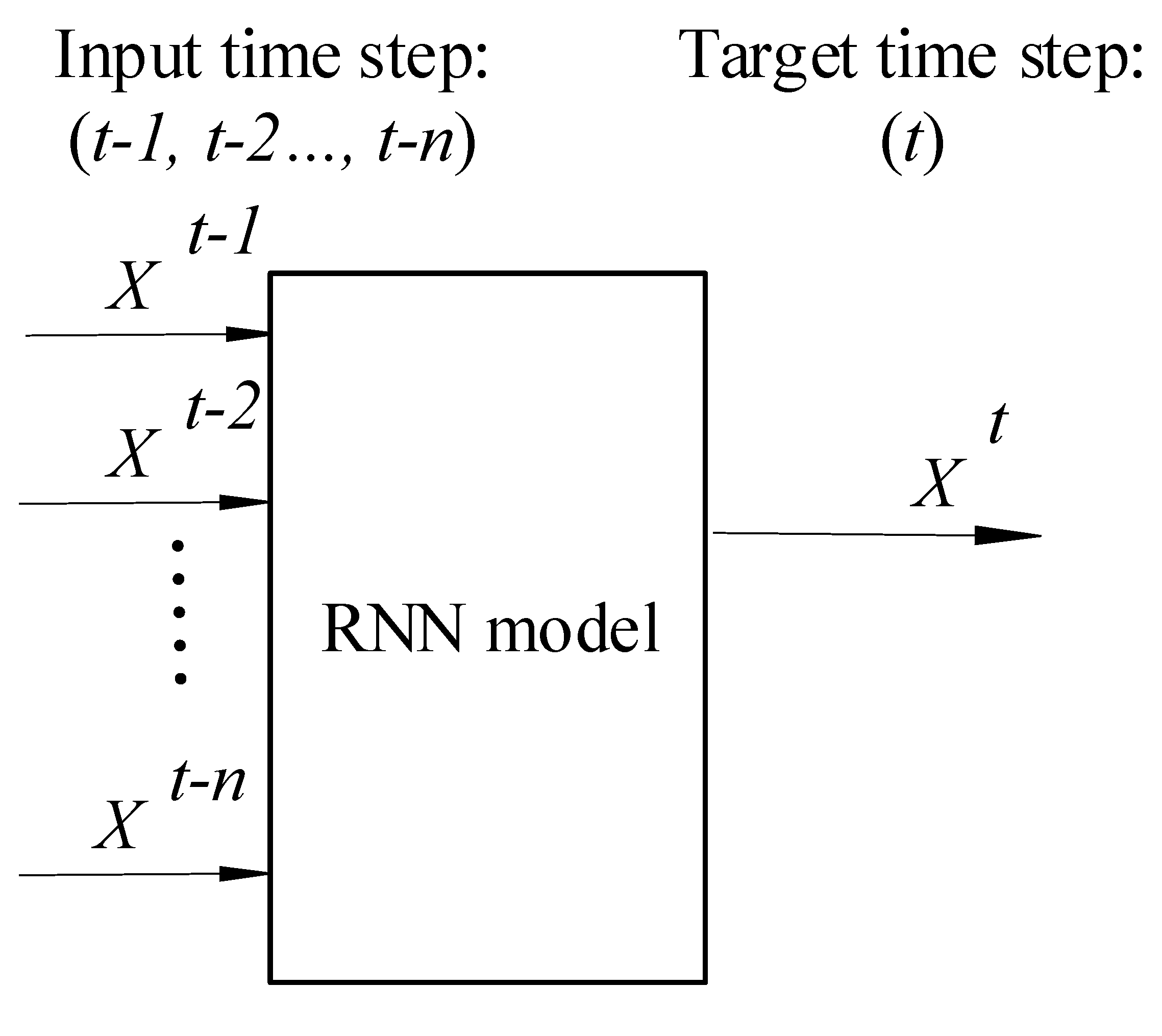
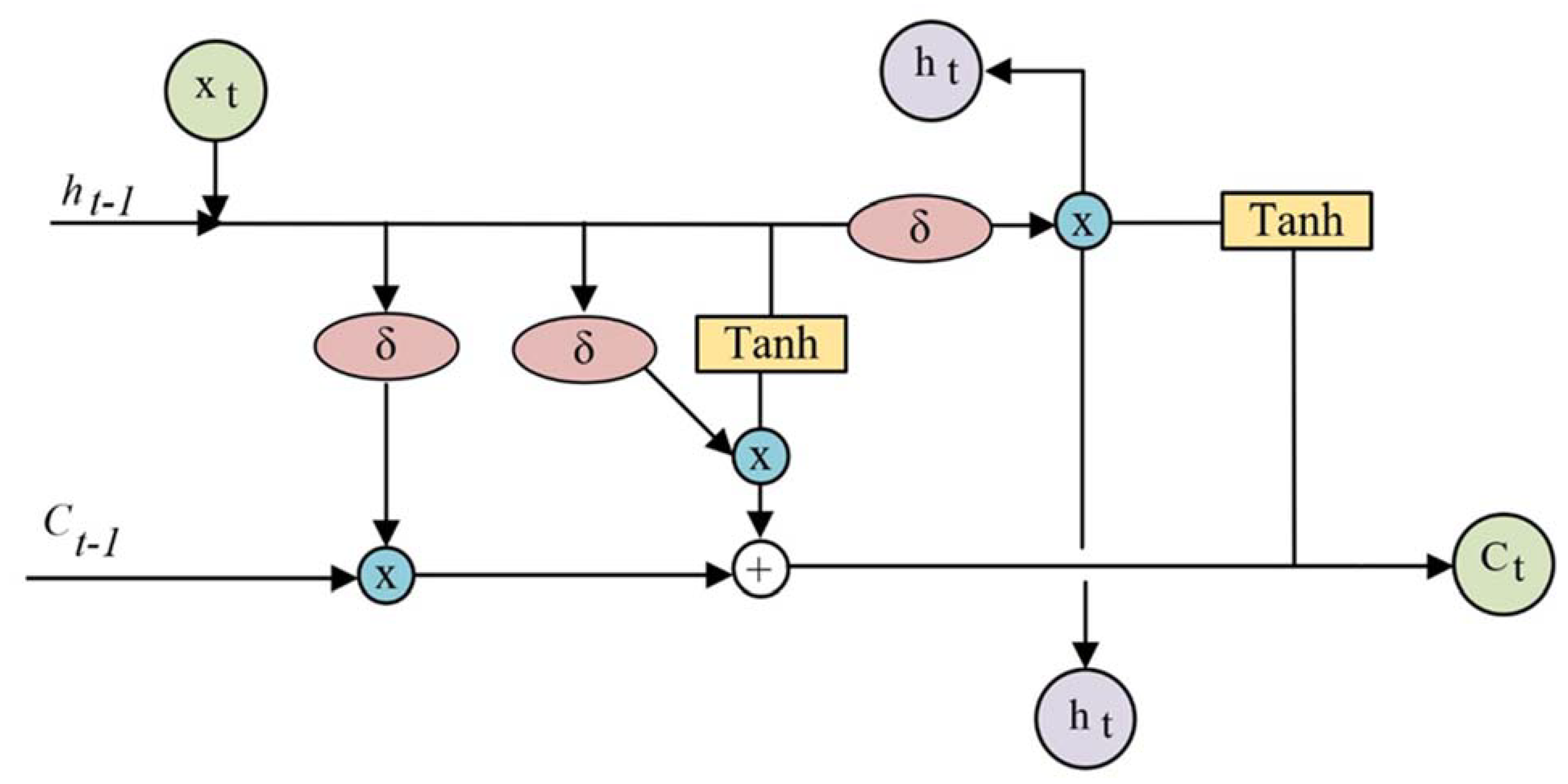
• The recurrent neural network (RNN), another deep learning method, which includes long-short-term memory (LSTM) architecture, was developed for multiple FDD using synthetic and measured databases [59]. The LSTM is capable of adding, storing and removing the information that is helpful for predictions [60].
• The PCA method, which is commonly used for dimension reduction and feature extraction [61,62], was applied using experimental data by [63,64] for single and multiple FDD in chillers and space heating and domestic hot water systems. Hybrid PCA models were applied for MFDD by [65,66,67,68].
• The naïve Bayes method was used for single and multiple FDD by [69,70].
• Clustering models were applied for multiple FDD of various HVAC systems by [71,72].

Compilation of MFDD models for HVAC systems from the literature review reveal the following trends [10,22,34,36,37,49,50,51,59,71,73,74,75,76,77,78,79,80,81]:

• Hybrid models accounted for 22% of the total number of studies, ANN and SVM accounted each for 22%, K-NN 17%, Bayesian network 11%, rule-based 5%, decision tree 5%, random forest 5%, clustering 5%, SVDD 5%, Deep ANN 5%, CNN 5%, and linear regression and linear discriminant analysis accounted each for about 5% of total publications.
• Measurements’ data were used in 67% of the publications, while synthetic data were used in 33%.
• About 44% of the publications focused on the FDD models for AHUs, 33% on chillers; other HVAC systems/components (i.e., whole HVAC system, packaged rooftop unit, and ground source heat pump) accounted each for 5% of studies.
• While most publications presented FDD methods for one faulty sensor, a smaller number of publications covered the multiple dependent FDD (sequential or concurrent) in HVAC systems.

In conclusion of the literature review, the data-driven techniques have the most attention for FDD in HVAC system, because they can be used if there is limited information about the system operation model. The black-box model is the most common model of the process history-based technique due to its simplicity, performance, and accuracy. However, the second most common technique was the rule-based model which is a qualitative-based model. The quantitative-based model is the least common popular method for FDD due to its complexity in development.

The summary of the strengths and weaknesses of the FDD models are represented in

Table 1. Strengths and weaknesses of FDD methods.

Model	Strengths	Weaknesses
Process history-based	- The models are well developed with just input and output of the system without knowing the physical system information (Black-Box). - Simplicity. - Good performance. - Applicable for non-linear systems.	- A large and reliable data set is required to develop an accurate model.
Qualitative model-based	- Simplicity for development and application. - No need to know the mathematical models of the system operation.	- Rules can be developed and applied for a specific system which the mode cannot be applied for other systems.
Quantitative model-based	- Accuracy on the target value prediction. - Capture steady and transient system operation. - Flexibility. - Generalisation with enough information, etc.	- Complexity of models. - Computationally intensive. - If there is not enough information of the system operation, the estimation of the target variable may not be accurate.

.

For development of the black-box models, selection of the correlated variables is so important to consider the effectiveness of the mode, the accuracy, and stability. For the HVAC system components, the system operation variables (air temperature, supply/ return water temperature, flow rate, etc.), environmental variable (temperature, etc.), time indicators (wee-days, weekend), and operation conditions (operation schedule, on/off) were potential correlated variables.

The model hyperparameter selection was another important aspect for the machine learning model developments. If a few parameters were used as the input data set, short training dataset and less hidden layer neurons were selected, the model may not be developed perfectly; in other words, it will be underfitted, i.e., the model has not been trained very well, and cannot predict the system performance. However, if many parameters and features were used as the input, and many hidden layer neurons in ANN model were selected, the model will be overfitted. The model was trained perfectly and predicts accurately in training set. However, prediction in the new (testing) dataset was not accurate.

The advantages and limitations of models were reported, and some are summarized here. This review section can be used as a guideline for development and application of models for detection and diagnosis of the multiple dependent faults in the components of the HVAC systems.

The novelty of this study for multiple dependent fault detection and diagnosis of air temperature sensors in the AHU is summarized below:

-

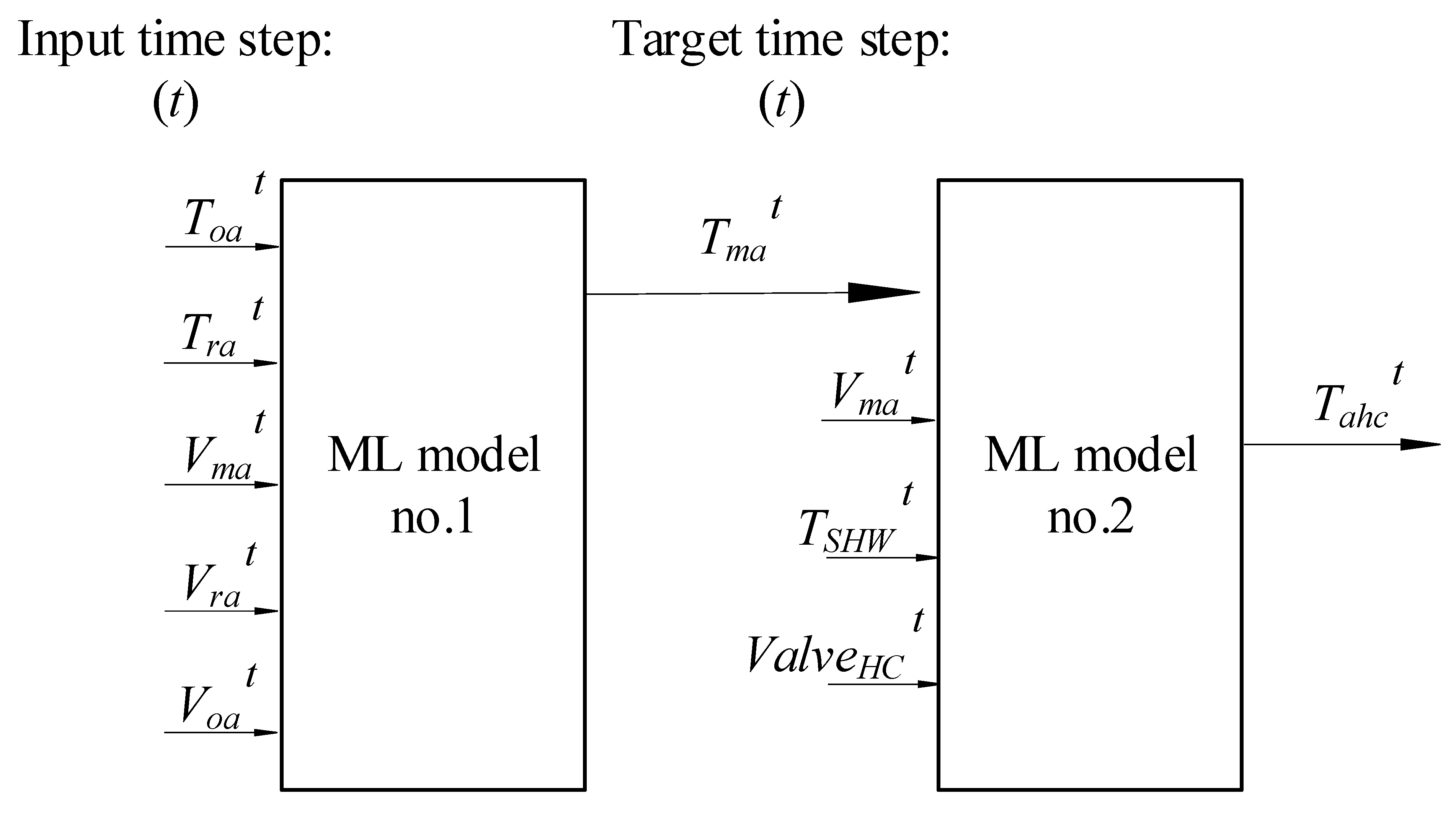
A novel sequential (compound) machine learning model for the prediction of the target variable (T_ma and T_ahc) in the AHU for the scope of MDFDD was proposed.

-

A novel technique for the threshold definition for the scope of MDFDD was proposed, which combines the sensor uncertainty and ML model uncertainty.

-

A hybrid technique, which combines machine learning models and rule-based techniques, was proposed for the MDFDD of the air temperature sensors in an AHU.

-

Different machine learning, deep learning, and hybrid models for the MDFDD scope were developed with the application of the K-fold cross validation of models.

This paper tests two hypotheses: (i) a combination of machine learning (ML) models using BAS trend data and rule-based models were successful in the multiple dependent faults detection and diagnosis (MDFDD) in the sensors of an AHU, and (ii) the information about relationship between sensors was essential for correctly detecting and diagnosing the faults.

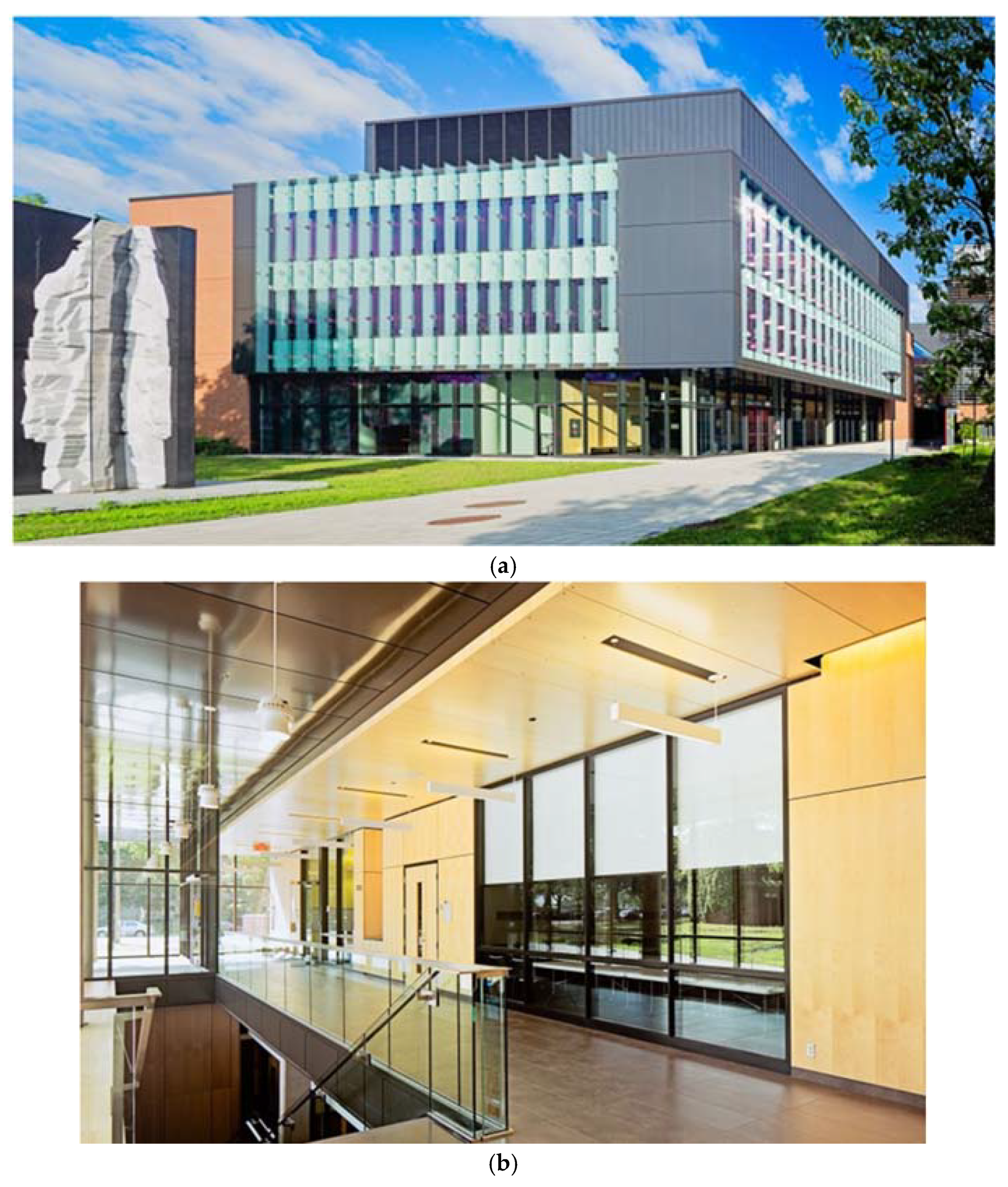
3. Case Study

The case study was an air handling unit of an institutional building, the Genomic building, with a total floor area of 5400 m², including three floors (Figure 1). The building was located in Montreal, Canada, with an orientation of 60° NW and a window-to-wall ratio of 33%. This building had 48 offices, three conference rooms and corridors which allocated for about 53% of the total floor area. The laboratories with the fume hoods accounted for 30% of the area, and the remaining areas were accounted for the kitchen (lounge) and restroom on each floor. The design capacity of the HVAC system was 42,472 L/s and 119.2 kW of electric power input to fans. More details are presented in [82,83].

Measurements used in this paper were recorded by 10 physical sensors (

Table 2. List of AHU variables.

No.	Variable	Description	Fixed (Bias) (Bx)	Random Error (Rx)	Total Uncertainty	Unit
1	Toa	Outdoor air dry-bulb temperature	0.45	0.19	0.49	°C
2	Tra	Return air temperature				°C
3	Tma	Mixed air temperature				°C
4	Tahc	Air temperature after heating coil				°C
5	Tsa	Supply air temperature				°C
6	TSHW	Supply hot water temperature	0.31	2.20	2.22	°C
7	Vma	Mixed air volumetric flow rate	222.0	506.11	552.65	L/s
8	Vra	Return air volumetric flow rate	222.0	229.84	319.55	L/s
9	Voa	Outdoor air volumetric flow rate	222.0	355.98	419.53	L/s
10	ValveHC	Heating coil valve position	-	-	2	%
11	ΔTs,fan	Air temperature rise over supply fan	-	-	-	°C

) at 15-min interval, over the heating season from 26 December 2016 to 29 January 2017. For comparison with measurements, four sensors were modelled: T_ma and T_ahc by using SVR models, and T_oa and T_ra by using RNN models.

In the air handling unit (Figure 2), the outdoor air at temperature T_oa and volumetric flow rate V_oa is mixed with recirculated air (removed from the building) at temperature T_ra and volumetric flow rate V_ra air flow rate. The mixed air has the temperature T_ma and volumetric flow rate V_ma = V_oa + V_ra, which equals the volumetric flow rate supplied to all building spaces. The heating coil heated the mixed air from T_ma to T_ahc, which was controlled by a thermostat connected with a hearing coil valve that regulated the heat water flow at temperature T_SHW.

The sensors uncertainty, calculated from fixed (bias) and random errors, was used to generate the threshold to detect and diagnose the multiple faults. The fixed (bias) and random errors for the sensor’s uncertainty were obtained from previous study of the same AHU [82,83].

4. Method

This paper proposes a method for the detection and diagnosis of multiple dependent faults of sensors of an AHU, by using a combination of machine learning (ML) models, which proved in the past good performance for linear and non-linear systems [4,84], and rule-based models. The ML models are developed from BAS trend data and implemented using Python (version 3.8.1) [30] with open-source libraries such as Scikit-learn [31], Keras [32], and Tensorflow [33].

One possible approach would consist of launching an exhaustive search, by using ML models, for detecting faults of all sensors in the AHU at time t. However, this is not an efficient solution.

The novelty of method proposed in this paper consists in the guidance for faults search, by considering the information and operation flow between sensors, and between sensors and devices. For this purpose, only two target sensors installed in the AHU are considered as the starting point (Figure 2), the mixed air temperature (T_ma) sensor, and the air temperature sensor after heating coil (T_ahc).

The following steps are implemented for the detection and diagnosis of the dependent multiple faults in the air temperature sensors of the AHU (Figure 3):

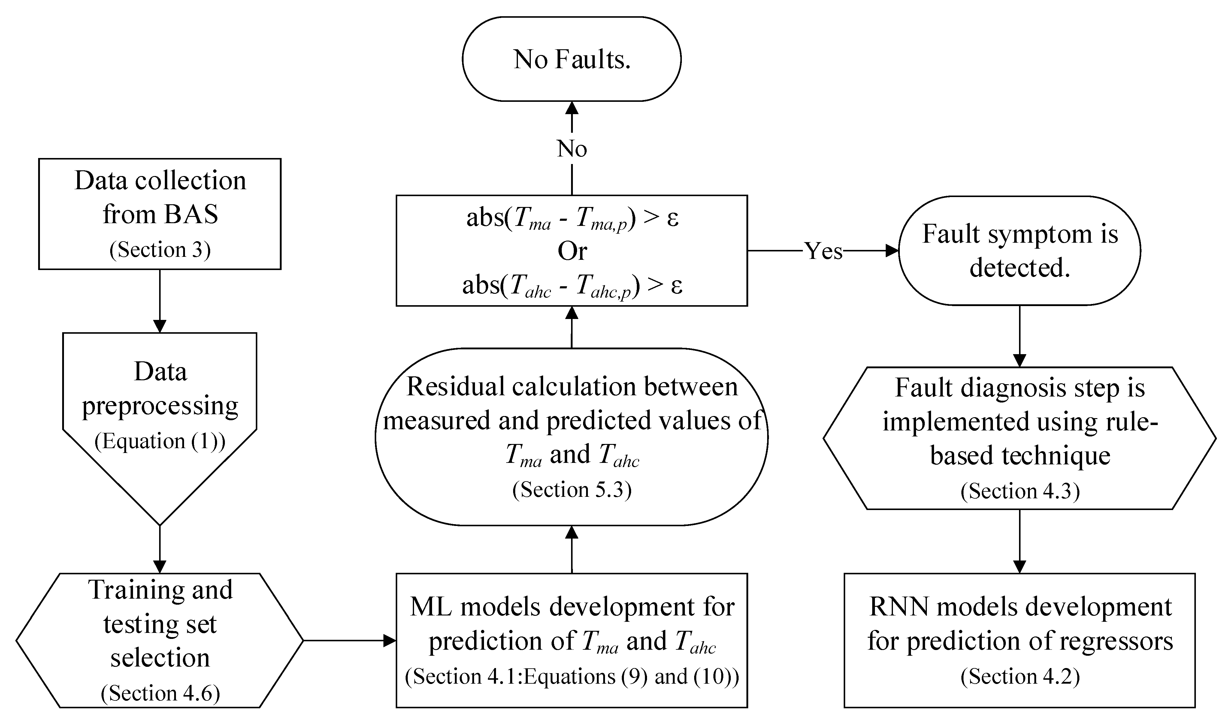
(1)

Data collection from BAS.

(2)

Data pre-processing for quality control, missing data, and data normalization. Measurements X that does not respect Equation (1) are removed.

(3)

Selection of training and testing data sets.

(4)

ML model development for the prediction of first target sensor (T_ma).

(5)

ML model development for the prediction of second target sensor (T_ahc).

(6)

Calculation of residuals between measured and predicted values of T_ma and T_ahc, respectively.

(7)

Detection of fault symptom.

(8)

Application of rule-based technique for the fault diagnosis step.

A compound ML model is proposed (Figure 4) that uses two distinct but related models (ML no.1 and ML no.2), one for the prediction of T_ma sensor value, and another for the prediction of T_ahc sensor value, each one measuring the impact of several inputs. Sensors that measure those independent inputs are called regressor sensors.

$${\mathsf{\mu }}_{dataset}-2\times { \mathsf{\sigma }}_{dataset}<\mathrm{X}<{\mathsf{\mu }}_{dataset}+2\times {\mathsf{\sigma }}_{dataset}$$

(1)

where, ${\mathsf{\mu }}_{dataset}$ is the average of the data set, ${\mathsf{\sigma }}_{dataset}$ is the standard deviation of the dataset, and $\mathrm{X}$ is the data point.

In this paper, the support vector regression (SVR) is developed to predict the mixed air temperature T_ma,p that corresponds to normal operation. If the residual (Res) of actual measurements of T_ma and predicted values (T_ma,p) exceeds the defined threshold ε, with positive or negative measuring bias, i.e., Res_ma = abs(T_ma − T_ma,p) > ε, the fault symptom for T_ma sensor is detected. Then the fault diagnosis method is activated.

The fault symptom could be generated by abnormal measurements of faulty target sensor, or by abnormal operation of other sensors/devices due to the improper control or degradation of performance. Therefore, one can ask the question: is the T_ma sensor faulty, and/or the regressor sensors (T_oa, T_ra, V_ma, V_ra, V_oa) are faulty (Figure 4)? If the regressor sensors are faulty, and T_ma sensor if not faulty, then a false symptom of T_ma sensor is detected.

To respond to this question, the recurrent neural network (RNN) is used for the fault symptom identification of regressor sensors. The value of each regressor sensor X at time t is predicted by using the past measured values at t-1, t-2, …, t-n (Figure 5). If the residual between actual measurements and predicted values, corresponding to normal operation of regressor sensor X, exceeds the defined threshold ε, the fault symptom of regressor sensor X is detected.

As an example, fault symptoms might be detected on two sensors, T_ma and T_oa. The diagnosis must clarify if both sensors are faulty, or only one sensor. If the fault symptom of regressor sensor T_oa is detected, the corrected sensor output T_ma,R under the influence of faulty T_oa is calculated by using a grey-box model, which is based on energy balance equation of mixing box (Equation (2)):

T_ma,R = a T_oa + b T_ra

(2)

where T_ma,R is the expected value of T_ma as affected by the faulty T_oa; a = V_oa/V_ma, and b = 1-a = V_ra/V_ma; coefficients a and b are identified by using the least square method (LSM) with training data set. For simplification, it is assumed that other regressor sensors are accurate.

If the residual of measurements of T_ma and corrected predicted values T_ma,R (Equation (2)) does not exceed the threshold ε, then T_ma is not a faulty sensor, but it signals the deviation due to the faulty T_oa. Hence, a false symptom of T_ma is detected. Therefore, only T_oa sensor is faulty. Similar approach is used for other regressor sensors such as T_ra. A few examples of rule-based diagnosis models are presented in Section 4.3.

The support vector regression (SVR) is also used to predict T_ahc,p that corresponds to normal operation, without known problems. If the residual (Res) of actual measurements of T_ahc and predicted values T_ahc,p exceeds the threshold ε, i.e., Res_ahc = (T_ahc − T_ahc,p) > ε, the fault symptom of T_ahc sensor is detected.

If the regressor sensor T_ma is faulty, the corrected sensor output T_ahc,R under the influence of faulty T_ma is calculated by using a grey-box model, which is based on energy balance equation of heating coil (Equation (3)):

$$T_{ahc,R}=\frac{\mathrm{c} T_{SHW}}{\mathrm{d} V_{ma}}+\mathrm{e} T_{ma}$$

(3)

where T_ahc,R is the expected value when T_ahc is affected by the faulty T_ma; and coefficients c, d and e are identified by using the least square method with training data set. If the residual of measured T_ahc and predicted T_ahc,R (Equation (3)) does not exceed the threshold, we can conclude that T_ahc is not faulty, but it signals the deviation due to the faulty T_ma. A few examples of rule-based diagnosis models are presented in Section 4.3.

The optimum hyperparameters of the RNN models were selected by using The RandomizedSearchCV method [31]: the number of hidden layers = 4, number of hidden neurons in each hidden layer = 50, the dropout regularization ratio = 0.2, and the sigmoid activation function. Ten time-lags of measurement are selected by random search as inputs of regressors.

4.1. Fault Symptom Detection Model Using Support Vector Regression (SVR)

Support vector regression (SVR) is a supervised machined learning model which comes from the support vector machine (SVM) for regression-based purposes [85,86,87,88]. The SVM model predicts the target value with the function of ($f$) by mapping using a nonlinear function ($\varnothing$), the data set of $x$ into a higher dimension feature space.

$$f\left(x\right)=\langle w, \varnothing \left(x\right)\rangle +b$$

(4)

where, $w$ is the matrix of regression coefficients, $b$ is the intercept, $x$ is the matrix of regressors.

The optimization model was proposed by Vapnik [89] to formulate function $f$ which includes regression coefficient ($w)$ and intercept $\left(b\right)$ to predict the target vectors $\left(y\right)$ with a precision of $\delta$.

$$\begin{gathered} mi{n}_{w,b,\xi ,{\xi }^{\ast }}\frac{1}{2}\Vert w^2\Vert +C{{\displaystyle \sum }}_{i=1}^l\left({\xi }_i+{\xi }_i^{*}\right) \\ \langle w, \varnothing \left(x_i\right)\rangle +b-y_i\le \delta +{\xi }_i , \\ {y}_i-\langle w, \varnothing \left(x_i\right)\rangle -b\le \delta +{\xi }_i , \\ {\xi }_i, {\xi }_i^{*}\ge 0,i=1,\dots ,l. \end{gathered}$$

(5)

where, $y_i$ is the target vector observation, ${\xi }_i$ is a slack variable, and $\delta$ and $C$ are the parameters that need to be selected through random search over a given range of values.

The regression function $f\left(x\right)$ and regression coefficients $\left(w\right)$ are presented in Equations (6) and (7).

$$f\left(x\right)=\left({\alpha }_i+{\alpha }_i^{*}\right)k\left(x_i,x\right)+b$$

(6)

$$w={{\displaystyle \sum }}_{i=1}^l\left({\alpha }_i+{\alpha }_i^{*}\right)x_i$$

(7)

where, ${\alpha }_i$ and ${\alpha }_i^{*}$ are the Lagrange multipliers and $k$ is the kernel function.

The kernel function is used for the distribution representation of input values of the training data set [90]. Radial basis function is used as the kernel function as represented in Equation (8).

$$k\left(x_i,x_j\right)=exp\left(-\gamma \Vert x_i-x_j\Vert {}^2\right)$$

(8)

where, $\gamma$ is the width parameter which reflects the variation range of all regressors in the training data set.

The values of required parameters ($\delta , C, \gamma$) are identified using the training data set, and thus the SVR model is developed. The predicted target values are obtained by using the testing data set.

The compound SVR models for the prediction of the T_ma and T_ahc are summarized by Equations (9) and (10).

$$T_{ma}{}^t=f\left(\begin{array}{c}{T}_{oa}{}^t,T_{ra}{}^t,V_{oa}{}^t, V_{ra}{}^t,V_{ma}{}^t\end{array}\right)$$

(9)

$$T_{ahc}{}^t=f\left(\begin{array}{c}{T}_{ma}{}^t,V_{ma}{}^t,T_{SHW}{}^t,Valv{e}_{HC}{}^t\end{array}\right)$$

(10)

4.2. Recurrent Neural Network (RNN) for Prediction of Regressor Sensors

In this paper, RNN models predict the values of correlated regressor sensors at time t by using the previous values at times t-1, t-2, …, t-n. These values are further used for the generation of expected target value (e.g., T_ma) as affected by faulty regressors (e.g., T_oa). This information was used for the fault symptom detection (see Section 4—Method). The RNN model is a deep learning model with long-short-term memory (LSTM) architecture that uses the previous sequential information to learn and predict the present values. LSTM architecture has the chain-like structure of the neural networks and is able to learn the long-term dependencies. The LSTM is capable of adding, storing and removing the information [61]. The internal schematic structure of the RNN with the LSTM algorithm is illustrated in Figure 6.

Where X _t is the input vector, h _t is the hidden layer or output vector, tanh is the tanh activation function and δ is the sigmoid activation function, and C _t is the state of cell.

The RNN models of regressors sensors are summarized by Equations (11)–(14). The regressor sensors values are predicted by the previous time step values. At this step, for the prediction of regressors, the individual sensors are used without consideration of the impact of other sensors.

$$T_{oa}{}^t=f\left(T_{oa}{}^{t-1}, T_{oa}{}^{t-2},\dots ,T_{oa}{}^{t-n}\right)$$

(11)

$$T_{ra}{}^t=f\left(T_{ra}{}^{t-1}, T_{ra}{}^{t-2},\dots ,T_{ra}{}^{t-n}\right)$$

(12)

$$T_{SHW}{}^t=f\left(T_{SHW}{}^{t-1}, T_{SHW}{}^{t-2},\dots ,T_{SHW}{}^{t-n}\right)$$

(13)

$$Valv{e}_{HC}{}^t=f\left(Valv{e}_{HC}{}^{t-1}, Valv{e}_{HC}{}^{t-2},\dots ,Valv{e}_{HC}{}^{t-n}\right)$$

(14)

4.3. Fault Diagnosis of Sensors Using Rule-Based Models

After the fault symptoms were detected for target and regressor sensors, some rule-based models were used to diagnose the potential causes of faults. A few examples of such rules are presented below. When some sensors or devices were identified as possibly faulty, physical investigation by the maintenance staff was needed. In the meantime, the values of T_ma,p, T_ra,p, T_oa,p, and T_ahc,p, which are predicted by SVR or RNN models (used as virtual sensors), could be used for the continuation of correct operation of AHU.

The values of regressor sensors (e.g., T_oa, T_ra) depended only on the previous values, and are not affected by other sensors. The reading of T_ma was affected by the regressor sensors, and this effect was introduced by the grey-box model.

A.

Group A of rule-based models

When the fault symptom of sensor T_ma was detected (i.e., Res_ma = abs(T_ma − T_ma,p) > ε), the following rules apply (for the simplification of explanation, all other regressor sensors are assumed to be correct):

• If Res_oa = abs(T_oa − T_oa,p) > ε, and Res_ma = abs(T_ma − T_ma,p) > ε, then both T_ma and T_oa sensors have fault symptoms.
• If Res_ra = abs(T_ra – T_ra,p) > ε, and Res_ma = abs(T_ma − T_ma,p) > ε, then both T_ma and T_ra sensors have fault symptoms.
• If Res_oa> ε, and/or Res_ra > ε, and Res_ma = abs(T_ma − T_ma,R) < ε, then T_ma sensor is not faulty; and T_oa and/or T_ra sensors are faulty.
• If Res_oa < ε, and/or Res_ra < ε, and Res_ma = abs(T_ma − T_ma,p) > ε, then only T_ma sensor is faulty.
• If Res_oa > ε, and Res_ra > ε, and Res_ma = abs(T_ma − T_ma,P) > ε, then all three sensors, T_oa, T_ra, and T_ma, are faulty.

Other rules can be used for the diagnosis of outdoor and return air flow dampers position.

B.

Group B of rule-based models

When the fault symptom of sensor T_ahc is detected with positive measuring bias Res_ahc = (T_ah − T_ahc,p) > ε, the corrected sensor output T_ahc,R under the influence of faulty T_ma is calculated, and the following rules apply:

• If Res = (T_ahc − T_ahc,R) < ε, then T_ahc sensor is not faulty.
• If Res = (T_ahc − T_ahc,R) > ε, then T_ahc sensor is faulty.
• If the heating coil valve position (Valve_HC) is recorded open with (Valve_HC − Valve_HC,p) < ε, abs(T_ma − T_ma,p) < ε, and (T_SHW − T_SHW,p) > ε, then the T_ahc sensor is possibly faulty, and/or the hot water temperature is too high.
• If (Valve_HC) is recorded open with (Valve_HC − Valve_HC,p) > ε, abs(T_ma − T_ma,p) < ε, and (T_SHW − T_SHW,p) < ε, then T_ahc sensor is possibly faulty, and/or the heating coil valve might be stuck opened.
• If (Valve_HC) is recorded open with abs(Valve_HC − Valve_HC,p) < ε, abs(T_ma − T_ma,p) < ε, and (T_SHW − T_SHW,p) < ε, the T_ahc sensor is possibly faulty with positive bias.
• If (Valve_HC) is recorded as closed, and abs(T_ma − T_ma,p) < ε, then Valve_HC and/or heating coil leaks.
• If (Valve_HC) is recorded open, and (T_ma − T_ma,p) > ε, then T_ma sensor and/or T_ahc sensor might be faulty.

4.4. Performance Evaluation

The performance of prediction models of target variables was evaluated with statistical indices (Equations (15)–(19)): Coefficient of determination (R²), root-mean-squared-error ($\mathrm{RMSE}$), mean absolute percentage error ($\mathrm{MAPE}$), mean bias error ($\mathrm{MBE}$), and maximum absolute error (${\mathrm{ME}}_{\max }$) [91,92].

$${\mathrm{R}}^2 \left[1-\frac{{{\displaystyle \sum }}_{i=1}^n{(y_i-{\widehat{y}}_i)}^2}{{{\displaystyle \sum }}_{i=1}^n{(y_i-{\overline{y}}_i)}^2}\right]\times 100$$

(15)

$$\mathrm{RMSE}=\sqrt{\frac{{{\displaystyle \sum }}_{i=1}^n{\left({\widehat{y}}_i-y_i\right)}^2}{n}}$$

(16)

$$\mathrm{MAPE}=\frac{1}{n}{{\displaystyle \sum }}_{i=1}^n\left|\frac{{\widehat{y}}_i-y_i}{y_i}\right|\times 100$$

(17)

$$\mathrm{MBE}=\frac{{{\displaystyle \sum }}_{i=1}^n\left({\widehat{y}}_i-y_i\right)}{n}$$

(18)

$${\mathrm{ME}}_{\max }=\left|{\widehat{y}}_i-y_i\right|$$

(19)

where, ${\widehat{y}}_i$ is the predicted value, $y_i$ is the measured value, and $\overline{y}$ is the average measured value over the selected time interval.

4.5. Fault Detection and Diagnosis Performance

The performance of MDFDD models was evaluated by using the accuracy, precision, and sensitivity measures (Equations (20)–(22)) [93,94,95]. Accuracy measured the number of correct predictions of faulty and normal readings, respectively, over the total number of predictions (Equation (20)). Precision measured the number of correct predictions of faults out of all predicted faulty readings (Equation (21)). Sensitivity measured the number of faults predictions out of all actual faults (Equation (22)).

$$\mathrm{Accuracy}=\frac{\mathrm{TP}+\mathrm{TN}}{\mathrm{TP}+\mathrm{TN}+\mathrm{FP}+\mathrm{FN}}100\%$$

(20)

$$\mathrm{Precision}=\frac{\mathrm{TP}}{\mathrm{TP}+\mathrm{FP}}100\%$$

(21)

$$\mathrm{Sensitivity}=\frac{\mathrm{TP}}{\mathrm{TP}+\mathrm{FN}}100\%$$

(22)

where, TP is number of true positives, e.g., the number of correctly predicted faults; FP is number of false positives, i.e., the incorrectly predicted faults; FN is number of false negatives, e.g., the incorrectly labelled data as no-fault; and TN is number of true negatives, e.g., the correctly labelled readings as no-fault. The confusion matrix (

Table 3. Confusion matrix for fault detection.

		True (Known) Faults
		Negative (0)	Positive (1)
Predicted faults	Negative (0)	TN	FP
	Positive (1)	FN	TP

) describes the classification of predicted faults compared with true (known) faults.

4.6. Optimization of Training Data Sets for Model Development

The size of training set and selection of models hyperparameters were optimized. The hyperparameters for the SVR model are δ, C, γ (Section 4.1). The hyperparameters for the development of optimized RNN models are the input time lags, size of training set, number of hidden layers, number of hidden neurons, and the dropout regularization ratio.

The developed ML models were optimized using RandomizedSearchCV tool [31]. This is a tool in the Scikit-learn package of Python, which randomly selects the hyperparameters out of the values and options assigned by the user, to obtain the optimum ML models for T_ma and T_ahc over k-fold cross validation.

The following steps are applied for the optimization of training data set size:

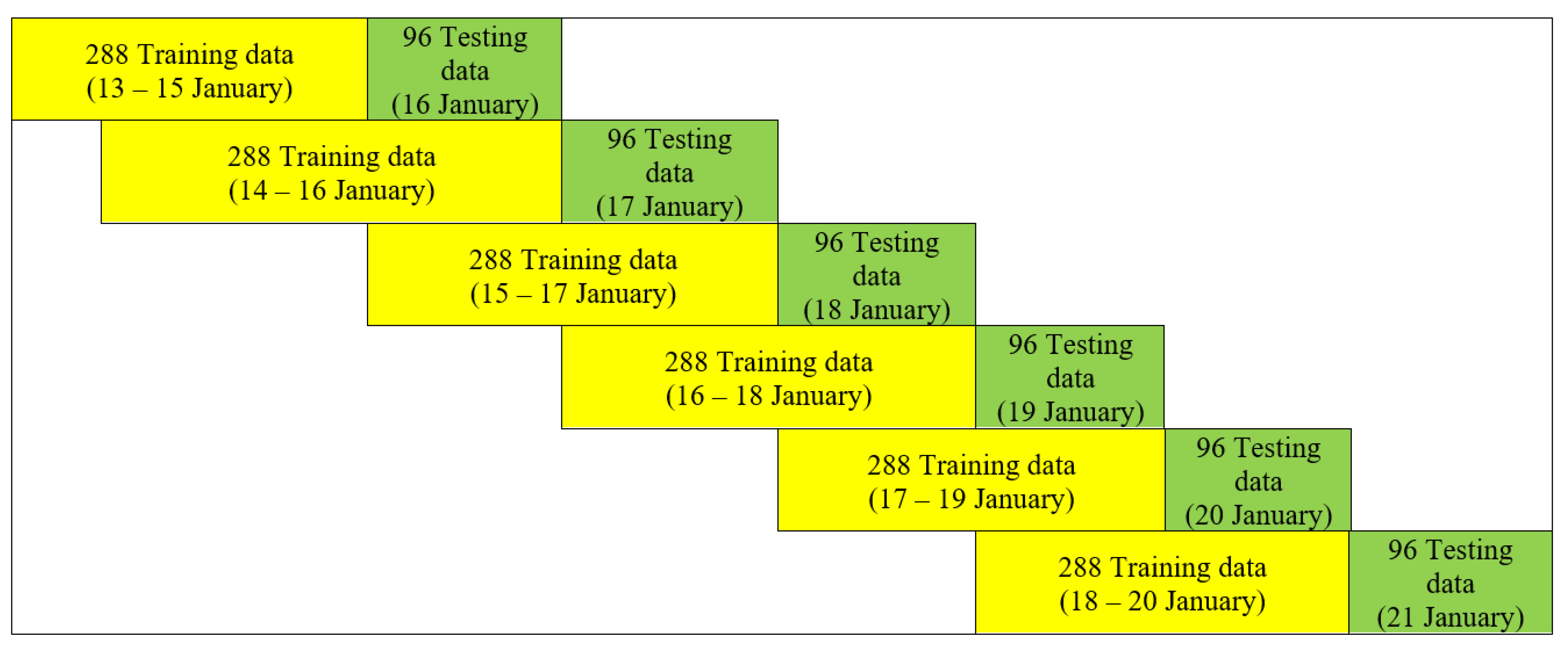
(a)

Let’s assume, for the purpose of explanation, the length of training the data set was three days, including 288 data points, from 13–15 January (Figure 7) and was tested with data from 16 January (96 data points). A new training data set was selected, with the same length of three days, by applying the sliding window technique, from 14–16 January, and tested with data of 17 January. In all, the sliding window moved over six consecutive days. Hence, the 6-fold cross validation used six different training data sets. The average RMSE value of predictions of T_ma over the corresponding testing data set was 0.41 °C. By using a similar approach, the average RMSE value of predictions of T_ahc was 0.21 °C.

(b)

The sliding window technique was implemented in this paper to evaluate the length of training data set over the course of consecutive days.

(c)

Results from different training data sets with lengths of 288, 480, 672, 864, 1,056, and 1,248 data points measured at 15-min intervals were compared. The optimum length of training a data set for the development of ML models of T_ma and T_ahc was composed of 288 data points.

(d)

The RandomizedSearchCV tool, including 10 cross-validation and 30 times for the number of iterations, was applied to obtain the optimum values for the hyperparameters of the SVR model for the T_ma and T_ahc. The optimum values for T_ma are C = 15.32 and γ = 0.015; and for T_ahc are C = 12.87 and γ = 0.057; the kernel was set to RBF for all SVR models.

5. Results and Discussion

This chapter presents the results of proposed MDFDD method with two different data sets: (i) a set with normal operation data, and (ii) a set with abnormal operation data.

5.1. Detection of Faults of T_ma Sensor under Normal Operation Conditions

Table 4. Prediction performance of SVR model of T_ma over training data set of three days and average testing results over the next six days.

Target	Input Variables	Prediction Performance of Model Over Training Data Set (288 Data Points)					Average of 6-Fold Cross-Validation of Prediction Performance Over Testing Data Set of One-Day (96 Data Points)
		R2 (%)	RMSE (°C)	MAPE (%)	MBE (°C)	$\mathbf{M}{\mathbf{E}}_{\mathbf{m}\mathbf{a}\mathbf{x}}$ (°C)	RMSE (°C)	MAPE (%)	MBE (°C)	$\mathbf{M}{\mathbf{E}}_{\mathbf{m}\mathbf{a}\mathbf{x}}$ (°C)
Tma	Toa, Tra, Vma, Vra, Voa	98.33	0.31	0.43	0.04	1.51	0.41	2.63	0.34	0.97

reports the average statistical indices from the prediction of T_ma by using the SVR model over six consecutive testing days (16–21 January). The threshold of 0.90 °C for fault detection is set by considering the sensor uncertainty and RMSE of model prediction.

The comparison of measured and predicted values of T_ma over testing data set is illustrated in Figure 8. A few fault symptoms were detected on 20 January, when the residual of measured and predicted values of T_ma exceeded the threshold of 0.90 °C. However, the anomaly of measurements was detected only for about 75 min, and then the measurements returned to normal values. Most likely, this symptom was created by staff entering the AHU for maintenance purpose. Therefore, no faults of T_ma were detected under normal operation conditions.

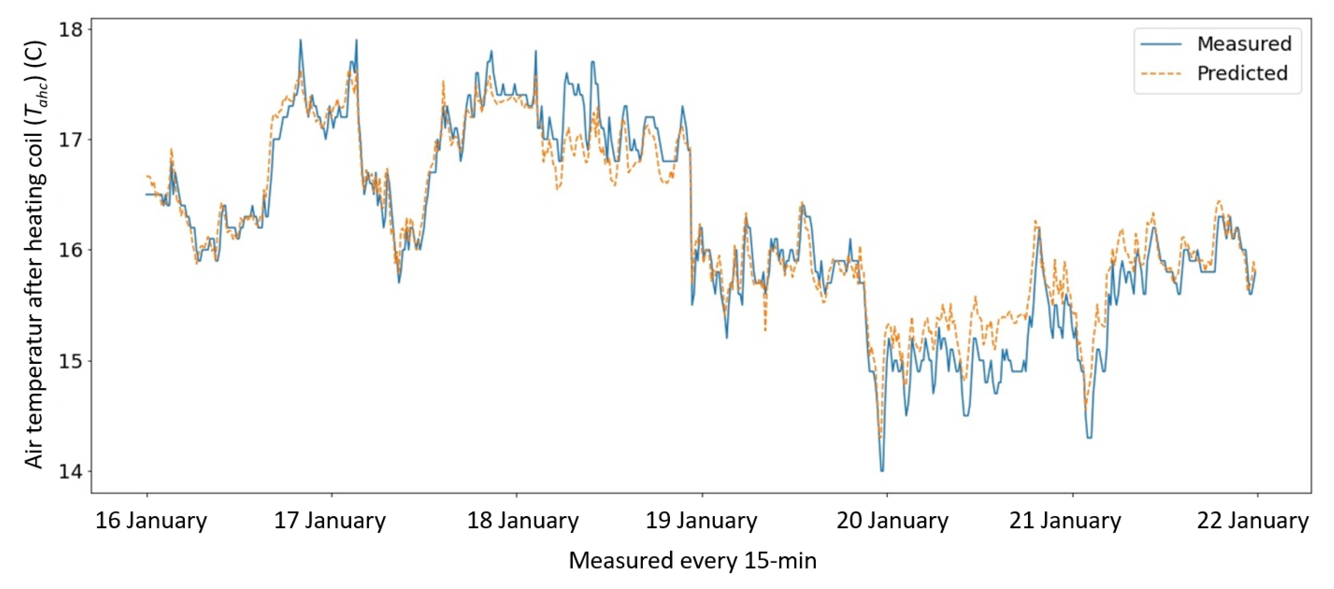
5.2. Detection of Faults of T_ahc Sensor under Normal Operation Conditions

Table 5. Prediction performance of SVR models of T_ahc over training data set of seven days and testing over the next day.

Target	Input Variables	Prediction Performance of Model Over Training Data Set (288 Data Points)					Average of 6-Fold Cross-Validation of Prediction Performance Over Testing Data Set of One-Day (96 Data Points)
		R2 (%)	RMSE (°C)	MAPE (%)	MBE (°C)	MEmax (°C)	RMSE (°C)	MAPE (%)	MBE (°C)	MEmax (°C)
Tahc	Tma, Vma, TSHW, ValveHC	98.83	0.16	0.14	0.02	0.57	0.21	1.08	0.17	0.60

reports the average statistical indices from the prediction of T_ahc over six consecutive testing days (16–21 January). The comparison of measured and predicted values of T_ahc over testing data set is illustrated in Figure 9. Since the residual of measured and predicted values of T_ahc did not exceed the threshold of 0.60 °C, no faults of T_ahc were detected.

Statistical indices of predictions of RNN models over normal operation conditions, and the threshold for each sensor are presented in

Table 6. Prediction performance of Recurrent Neural Network for selected regressors sensors.

Regressor Sensor at Time ‘t’	Average of 6-Fold Cross-Validation of Prediction Performance Over Testing Data Set of One Day (96 Data Points)					Threshold for Fault Detection
Variable	Unit	RMSE	MAPE (%)	MBE	$\mathbf{M}{\mathbf{E}}_{\mathbf{m}\mathbf{a}\mathbf{x}}$	ɛ = Sensor Uncertainty + RMSE
Toa	°C	0.89	100.03	1.98	3.42	1.38
Tra	°C	0.08	0.91	0.20	0.38	0.57
TSHW	°C	0.70	4.75	1.99	2.74	1.00
ValveHC	%	1.41	10.72	4.61	3.79	3.41

.

5.3. Detection and Diagnosis of Faults from Abnormal Operation Data

As in most cases of measurements from BAS, the available data set does not contain enough abnormal operation data that are due to sensor faults. In absence of faulty data, artificial faults of sensors were inserted in the testing data set of T_oa and T_ra. In addition, a grey-box model (Equation (2)) was applied to predict the target sensor T_ma output as induced by the artificial faults of T_oa and T_ra (

Table 7. Grey-box model for prediction T_ma as influenced by regressor sensors T_oa and T_ra.

No.	Model	Training Data Set (288 Data Points (3-Days))					Test Data Set (96 Data Points (1-Day))
		Parameter	Value	Unit	R2 (%)	RMSE (°C)	R2 (%)	RMSE (°C)
1	Equation (2)	a	0.204	-	92.24	0.53	95.98	0.55
		b	0.796	-

).

In a similar way, the relationship between the target sensor T_ahc and regressor sensors (Equation (3)) was applied.

One example of application of proposed method of MDFDD using artificial faults is presented in this section. Artificial faults were generated by adding to actual measurements of T_oa and T_ra a bias error of 0.5 °C on 19 January at 12:01 a.m., followed by a ramp of 0.02356 C/time step until 21 January at 12:00 a.m. (Figure 10 and Figure 11).

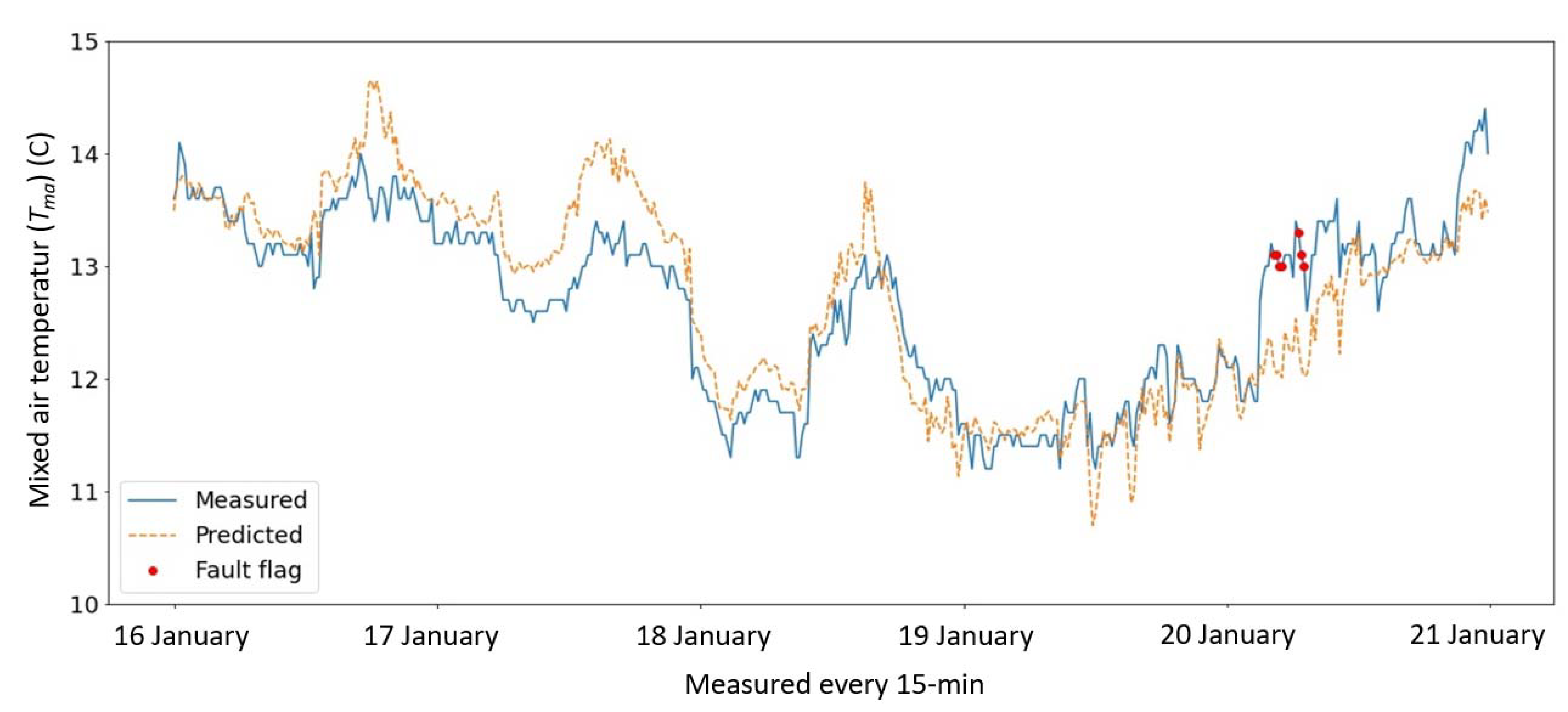
5.3.1. Detection of Fault Symptoms

The T_ma,p value expected to be measured under normal operation (Figure 12) was predicted by the SVR model. Since the residual of measured values (i.e., due to artificial faults) of T_ma and predicted values T_ma,p exceeded the threshold ε = 0.90 °C, a fault symptom of T_ma sensor was detected (Figure 13). Is the sensor T_ma faulty, or is the T_ma sensor correct under the influence of regressor sensors T_oa and T_ra?

5.3.2. Diagnosis of Faults

(1)

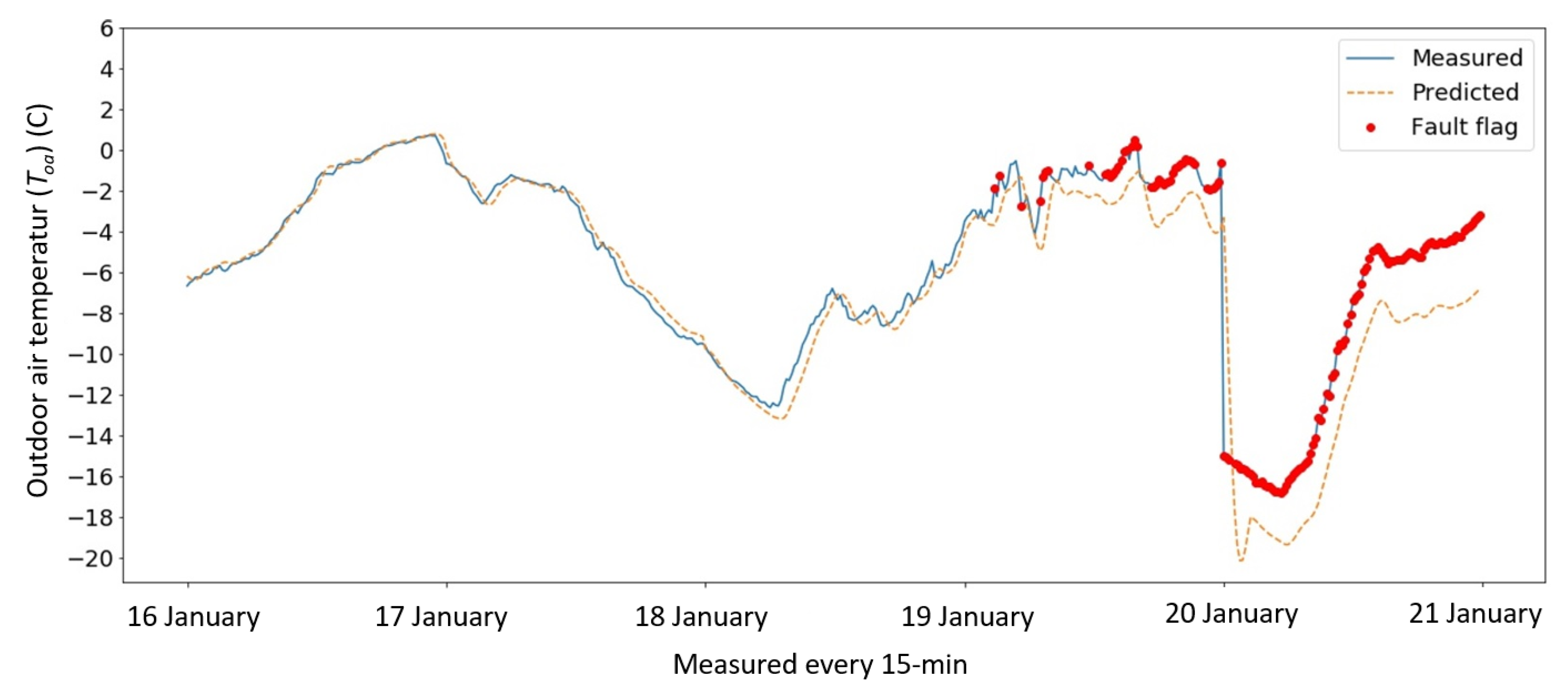
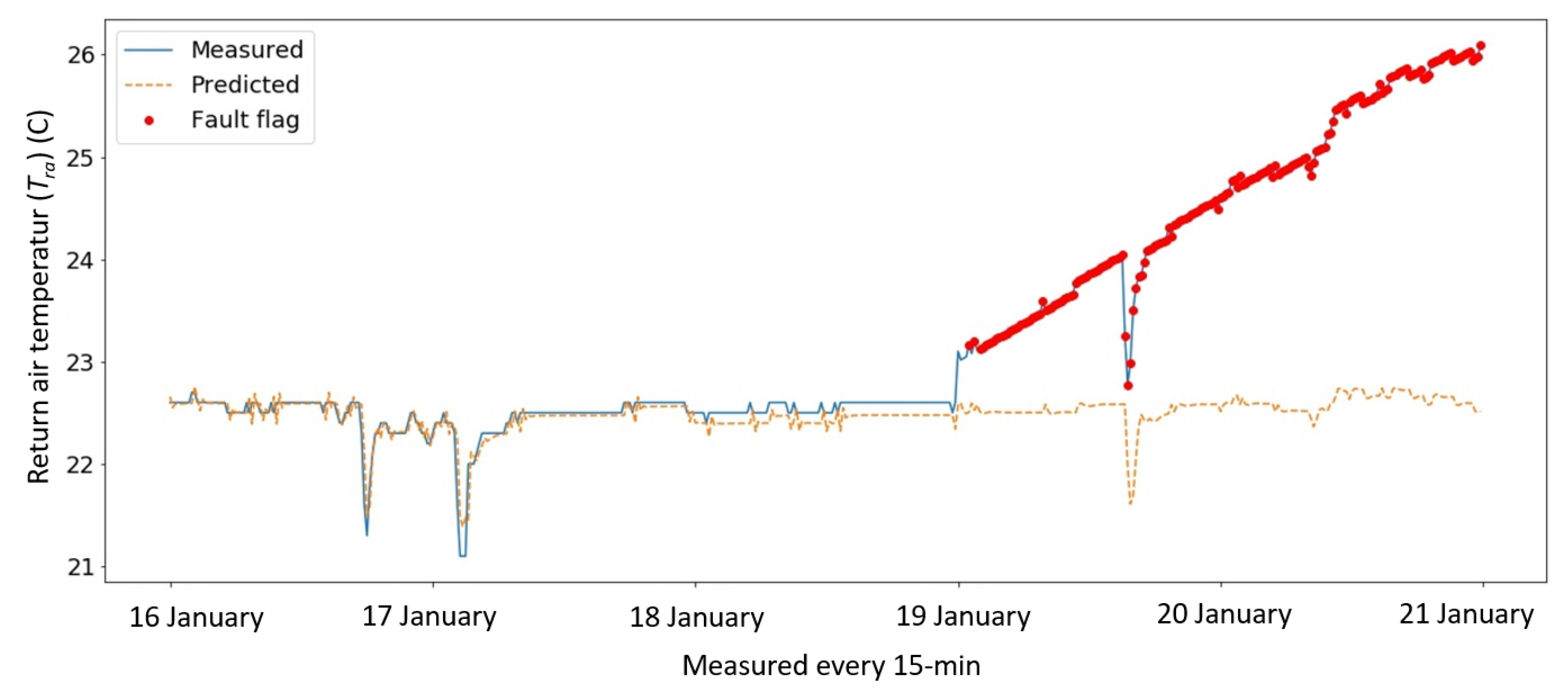
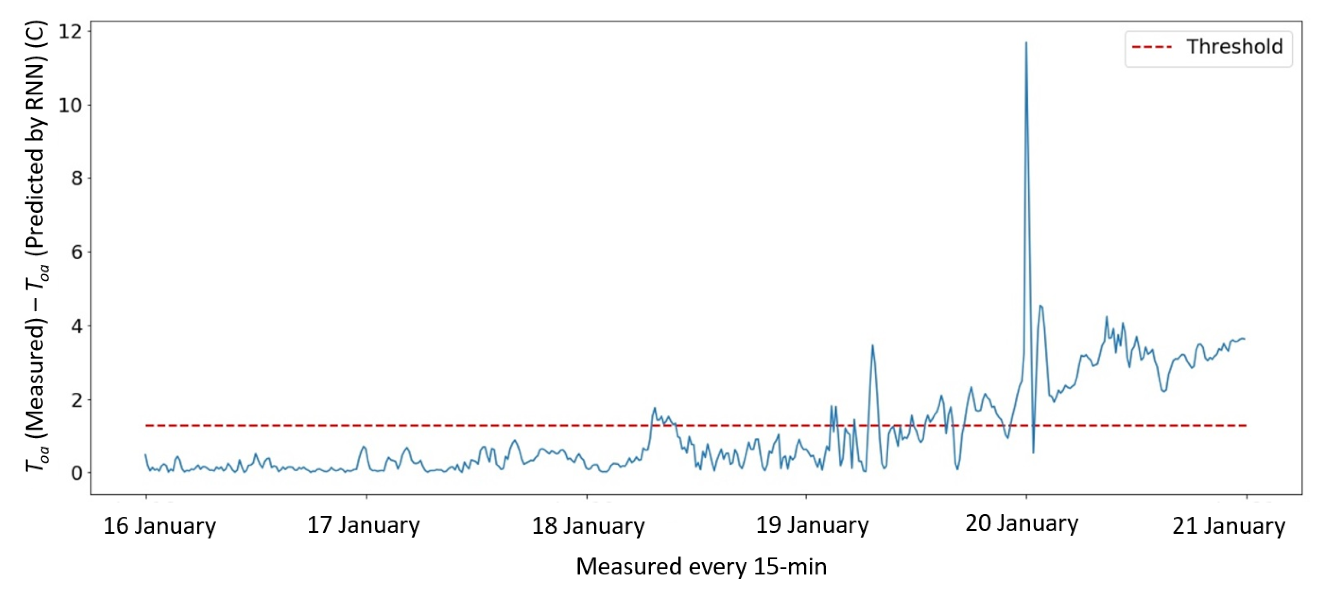
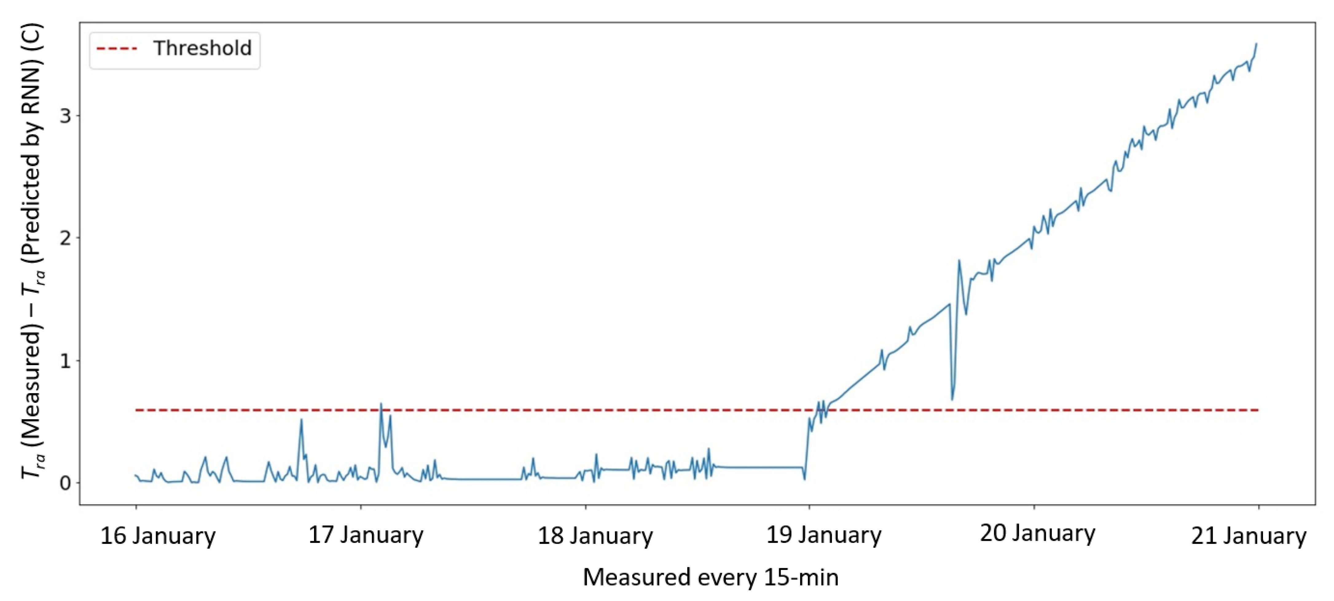
When the fault symptom of T_ma sensor was detected, the next step consisted of the analysis of regressor sensors T_oa and T_ra. RNN models predicted the values of T_oa,p and T_ra,p under normal operation conditions. When the residuals exceeded the threshold (i.e., Res_oa = abs(T_oa − T_oa,p) > ε, and Res_ra = abs(T_ra − T_ra,p) > ε), the fault symptoms of T_oa and T_ra were detected (Figure 14 and Figure 15).

Out of 160 artificial faults of T_oa, 138 faults were detected correctly (

Table 8. Confusion matrix for fault detection of T_oa.

		Actual Faults
		Normal (0)	Faulty (1)
Predicted faults	Normal (0)	311	22
	Faulty (1)	9	138

). Out of 189 artificial faults of T_ra, 187 faults were detected correctly (

Table 9. Confusion matrix for fault detection of T_ra.

		Actual Faults
		Normal (0)	Faulty (1)
Predicted faults	Normal (0)	289	2
	Faulty (1)	2	187

). The accuracy, precision, and sensitivity of the RNN models had values greater than 86% for T_oa, and around 99% for T_ra (

Table 10. Performance of MDFDD models: accuracy, precision and sensitivity.

Target	Prediction Performance of Model over Testing Data Set (6-Days, 576 Data Points)
	Accuracy (%)	Precision (%)	Sensitivity (%)
Toa	93.54	86.25	93.88
Tra	99.16	98.95	98.95

).

Therefore, T_oa and T_ra sensors were detected as faulty, which corresponded to artificial faults inserted in the data set.

(2)

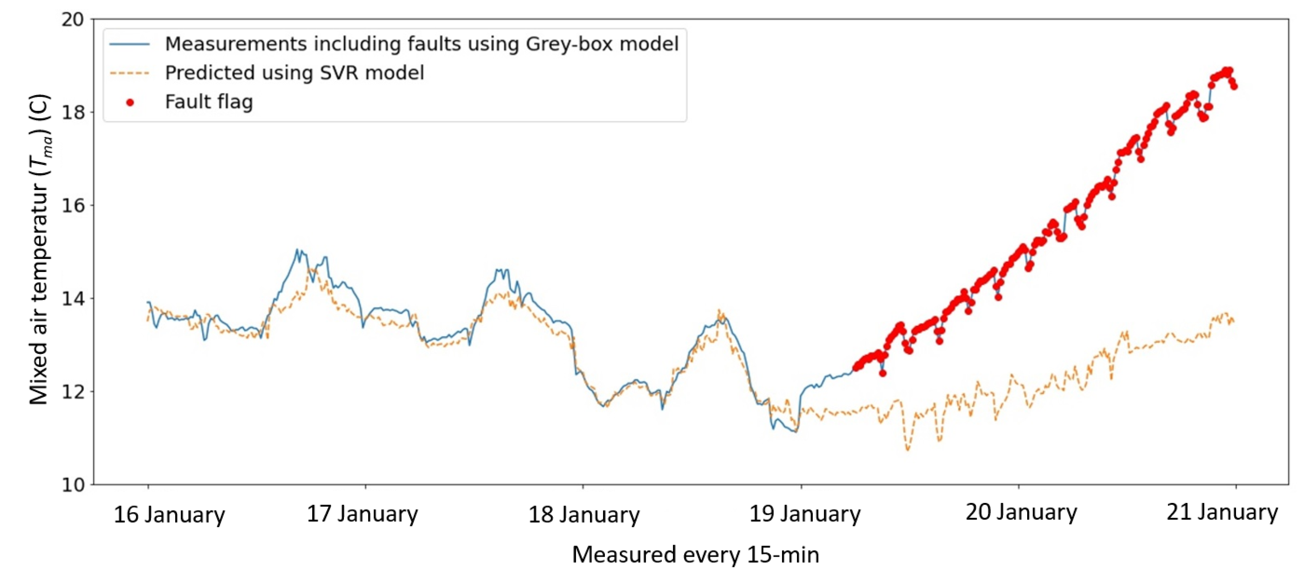
The expected output of T_ma,R under the influence of faulty T_oa and T_ra sensors was calculated by using a grey-box model (Equation (2), with coefficients a and b of Table 7.

(3)

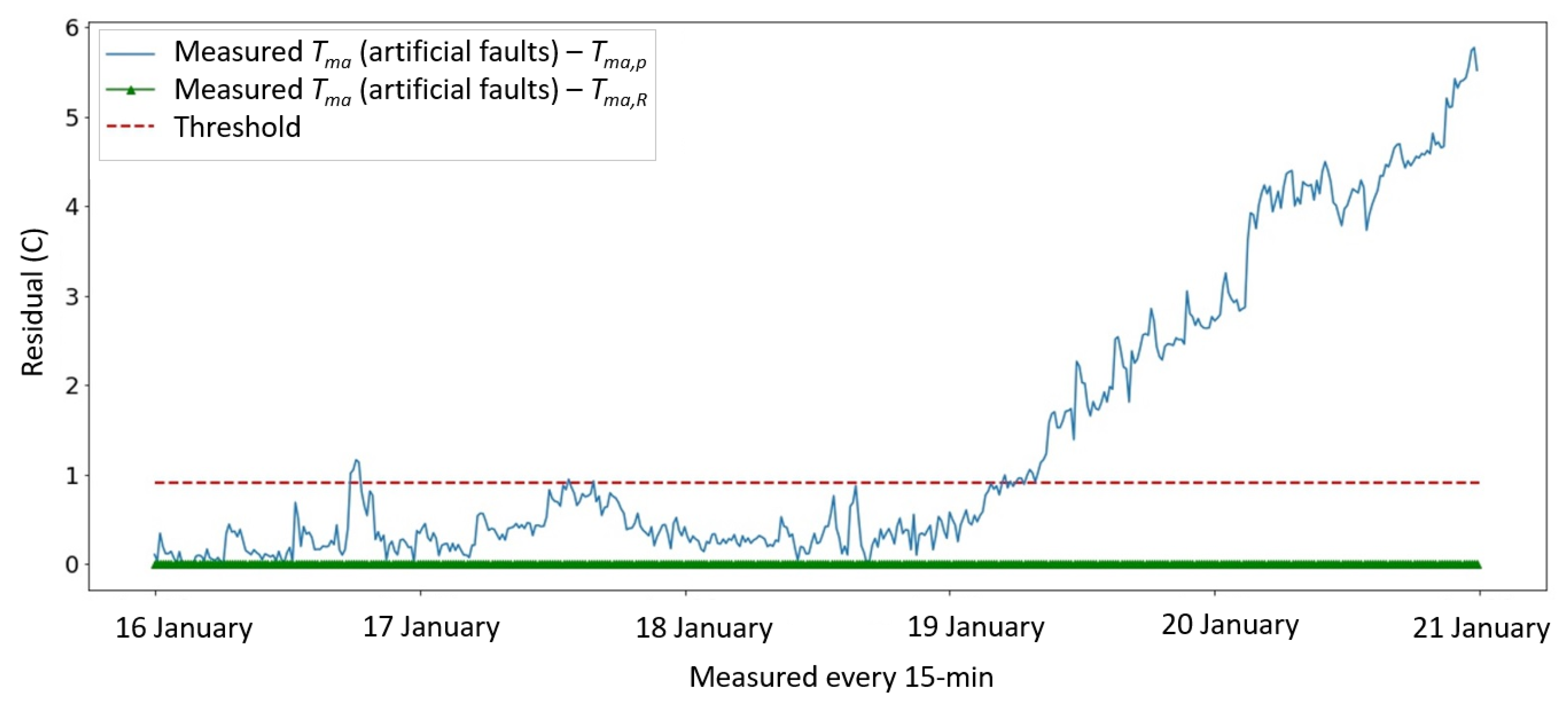
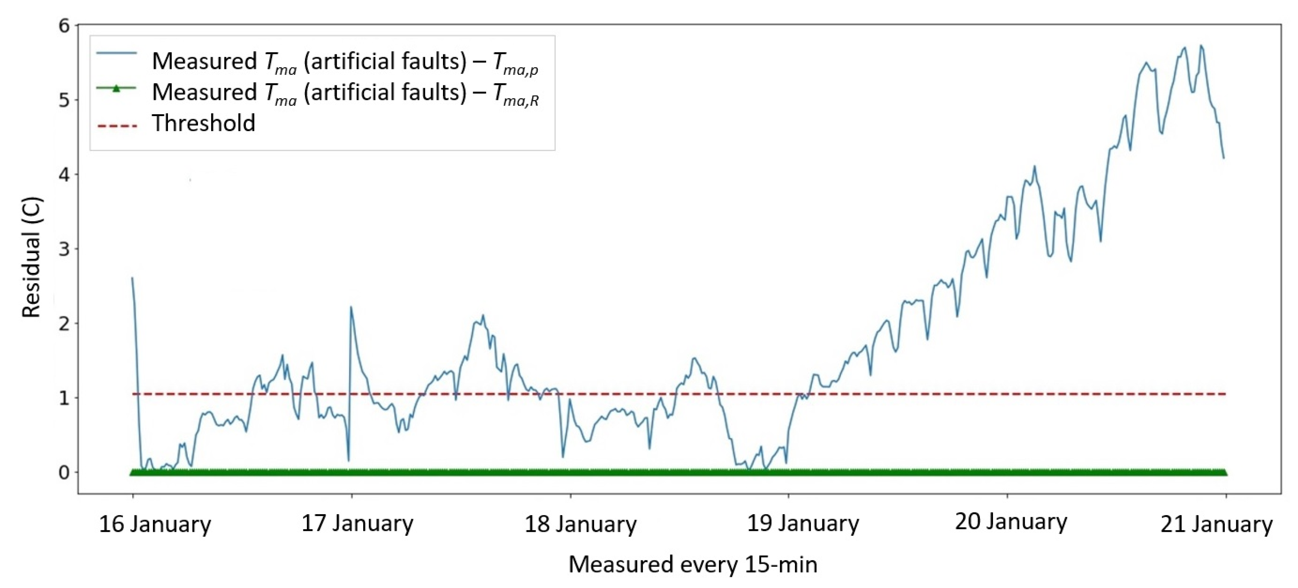
Since the residual of measured values (i.e., due to artificial faults) of T_ma and predicted values T_ma,R did not exceeds the threshold ε, the T_ma sensor was not faulty (Figure 13), and, thus, a false symptom was detected.

(4)

According to rule A.c. (Section 4.3), if T_oa and T_ra sensors were faulty, but the residual Res_ma = abs(T_ma − T_ma,R) < ε, then T_ma sensor was not faulty; only T_oa and/or T_ra sensors were faulty.

In conclusion of this example, without this approach, all three sensors T_ma, T_oa, and T_ra, would be wrongly considered as faulty.

If, in another case, the residual of measurements and predictions of T_ma, T_oa, and T_ra, respectively, exceeded the threshold, we could conclude that all three sensors (T_ma, T_ra, T_ma) had fault symptoms.

5.4. Comparison with Another Method

For comparison, this section presents the detection of faults by RNN models applied to all three sensors T_ma, T_ra, T_ma, but without any information about the relationship between sensors (

Table 11. Prediction performance of Recurrent Neural Network for selected regressors sensors.

Regressor Sensor at Time ‘t’	Average of 6-Fold Cross-Validation of Prediction Performance over Testing Data Set of One Day (96 Data Points)					Threshold for Fault Detection
Variable	Unit	RMSE	MAPE (%)	MBE	$\mathbf{M}{\mathbf{E}}_{\mathbf{m}\mathbf{a}\mathbf{x}}$	ɛ = Sensor Uncertainty + RMSE
Toa	°C	0.89	100.03	1.98	3.42	1.38
Tra		0.08	0.91	0.20	0.38	0.57
Tma		0.55	14.04	2.82	1.71	1.04

).

In addition of residuals obtained from the use of RNN models for T_oa and T_ra sensors (Figure 14 and Figure 15), Figure 16 shows the residual of T_ma obtained from RNN model applied to artificial faults. One can conclude that, by using RNN models without any information between sensors, the results showed that all three sensors were faulty, which is not true.

In conclusion, the proposed MDFDD method detected the faulty sensors, while the broad application of ML models to all sensors, without any information between the dependent sensors, did not detect correctly the faulty sensors.

6. Conclusions, Contributions, and Limitations

6.1. Conclusions

In this paper, the application of hybrid models was proposed, which combines the machine learning models and rule-based techniques for the detection and diagnosis of multiple depended faults of air temperature sensors of an AHU of an institutional building. Hybrid models were developed and evaluated using experimental data.

The results were summarized as follows:

-

The combination of machine learning (ML) models using BAS trend data, and rule-based models was successful for the multiple dependent faults detection and diagnosis (MDFDD).

-

The information about relationship between sensors was essential for the correct detection and diagnosis of dependent faults. For this purpose, a novel method that guides for faults search by using the information and operation flow between sensors, and between sensors and devices was presented. This approach was not found in any other publication.

-

ML models were used for the prediction of two target variables, the mixed air temperature (T_ma) and air temperature after heating coil (T_ahc). The RNN models were used for the prediction of regressor sensors values (T_oa, T_ra, T_SHW, Valve_HC). Rules-based models were used for the diagnosis of faults. These results revealed good performance of these models for the fault detection and diagnosis purposes.

-

The proposed method was tested with measurements from BAS trend data under normal operation, and with artificial faults inserted in the measurements data file. The results revealed good performance of the proposed method for the multiple dependent faults of air temperature sensors of an AHU.

-

Three days of training data with 288 data points recorded every 15-min was enough for the development of the SVR models for the prediction of target sensors (T_ma and T_ahc). RMSE over training and testing data sets were 0.31 °C and 0.41 °C, respectively, for the prediction of T_ma, and 0.16 °C and 0.21 °C, respectively, for the prediction of T_ahc.

-

The accuracy of models for the fault prediction of air temperature sensors of T_oa and T_ra was 93.54 and 99.16%, respectively.

6.2. Contributions

The contributions are listed as follows:

-

A novel sequential (compound) machine learning model for the prediction of the target variables (T_ma and T_ahc) for the scope of MDFDD was proposed.

-

A hybrid technique that combines machine learning models and rule-based techniques was proposed.

-

A new definition of threshold value was applied, which combined the sensor uncertainty and the ML model uncertainty.

-

Machine learning models were developed using the K-fold cross validation.

-

Models hyperparameters were optimized using RandomizedSearchCV tool.

6.3. Limitations

-

The proposed method should be tested over several heating season data sets and compared with physical faults detected by the maintenance team and recorded in workbooks.

-

Ideally, all sensors used in such a study should be periodically re-calibrated to ensure high quality of measurements. However, we understand that such a re-calibration is not always possible, when considering that the operation team had sometimes more urgent and essential calls for fixing HVAC systems.

-

Oher approaches should be used for the generation of artificial faults. The use of real experimental data from faults was important.

-

The work presented in this paper focused on the detection and diagnosis of multiple dependent faults of air temperature sensors. The work will be expanded by including faults of actuators and components of HVAC systems.

-

The machine learning models (SVR and RNN) have been developed using Python with application of the open source scikit-learn, Keras, and TensorFlow packages. A laptop with the following configuration was used: Windows 10, Intel(R) Core (TM) i5-1035G7 CPU @ 1.20GHz, 1498 Mhz, 4 Cores, 8 Logical Processors, and 8 GB RAM. The system was sufficient in development and optimization of the proposed ML models, taking no more than 60 s for SVR and 10 min for RNN models’ development. However, for the development of RNN models with more data and other optimization methods, longer computing time was expected. Hence, a more powerful computer was needed.

7. Future Works

The proposed method will be extended: (1) to other sensors of the AHU (e.g., volumetric air flow rate, water flow rate) and to other HVAC systems configuration and controls; (2) by using other ML models such as artificial neural network (ANN), decision tree regression, random forest regression model, and principal component analysis (PCA); (3) as an application software of building automation system (BAS) of HVAC systems, to trigger alarms for potential abnormal operation; and (4) as a portable online software for smartphones to control remotely the operation of the HVAC system in the commercial buildings.

References

- Beiter, P.; Elchinger, M.; Tian, T. 2016 Renewable Energy Data Book; National Renewable Energy Lab. (NREL): Golden, CO, USA, 2017. [Google Scholar]
- Katipamula, S.; Brambley, M.R. Review Article: Methods for Fault Detection, Diagnostics, and Prognostics for Building Systems—A Review, Part I. HVAC&R Res. 2005, 11, 3–25. [Google Scholar]
- Yua, Y.; Woradechjumroena, D.; Yub, D. A review of fault detection and diagnosis methodologies on air-handling units. Energy Build. 2014, 82, 550–562. [Google Scholar] [CrossRef]
- Kim, W.; Katipamula, S. A review of fault detection and diagnostics methods for building systems. Sci. Technol. Built Environ. 2018, 24, 3–21. [Google Scholar] [CrossRef]
- Cengel, Y.; Boles, M.A. Thermodynamics, An Engineering Approach, 6th ed.; McGraw Hill: New York, NY, USA, 2001. [Google Scholar]
- Zhao, Z.; Wang, S.; Xiao, F.; Ma, Z. A simplified physical model-based fault detection and diagnosis strategy and its customized tool for centrifugal chillers. HVAC & R Res. 2013, 19, 283–294. [Google Scholar]
- Liang, J.; Du, R. Model-based Fault Detection and Diagnosis of HVAC systems using Support Vector Machine method. Int. J. Refrig. 2007, 30, 1104–1114. [Google Scholar] [CrossRef]
- Pourariana, S.; Wen, J.; Veronica, D.; Pertzborn, A.; Zhouc, X.; Liu, R. A tool for evaluating fault detection and diagnostic methods for fan coil units. Energy Build. 2017, 136, 151–160. [Google Scholar] [CrossRef] [Green Version]
- Mulumba, T.; Afshari, A.; Yana, K.; Shena, W.; Norford, L.K. Robust model-based fault diagnosis for air handling units. Energy Build. 2015, 86, 698–707. [Google Scholar] [CrossRef]
- Bonvini, M.; Sohn, M.D.; Granderson, J.; Wetter, M.; Piette, M.A. Robust on-line fault detection diagnosis for HVAC components based on nonlinear state estimation techniques. Appl. Energy 2014, 124, 156–166. [Google Scholar] [CrossRef]
- Najafi, M. Modeling and Measurement Constraints in Fault Diagnostics for HVAC Systems; Lawrence Berkeley National Laboratory, University of California: Berkeley, CA, USA, 2010. [Google Scholar]
- Najafi, M.; Auslander, D.M.; Bartlett, P.L.; Haves, P.; Sohn, M.D. Application of machine learning in the fault diagnostics of air handling units. Appl. Energy 2012, 96, 347–358. [Google Scholar] [CrossRef]
- Wang, H.; Chen, Y.; Chan, C.W.H.; Qin, J.; Wang, J. Online model-based fault detection and diagnosis strategy for VAV air handling. Energy Build. 2012, 55, 252–263. [Google Scholar] [CrossRef]
- Deshmukh, S.; Glicksman, L.; Norford, L. Case study results: Fault detection in air-handling units in buildings. Adv. Build. Energy Res. 2018, 14, 305–321. [Google Scholar] [CrossRef]
- Schein, J.; Bushby, S.T.; Castro, N.S.; House, J.M. A rule-based fault detection method for air handling units. Energy Build. 2006, 38, 1485–1492. [Google Scholar] [CrossRef]
- Schein, J. Results from Field Testing of Embedded Air Handling Unit and Variable Air Volume Box Fault Detection Tools; U.S. Department of Commerce, National Institute of Standards and Technology: Gaithersburg, CA, USA, 2006.
- Katipamula, S.; Brambley, M.R.; Luskay, L. Automated Proactive Techniques for Commissioning Air handling unit. Sol. Energy Eng. Trans. ASME 2003, 125, 282–291. [Google Scholar] [CrossRef]
- House, J.M.; Vaezi-Nejad, H.; Whitcomb, J.M. An expert rule set for fault detection in air handling units. ASHRAE Trans. 2001, 107, 858–871. [Google Scholar]
- House, J.M.; Lee, W.Y.; Dong, R.S. Classification techniques for fault detection and diagnosis of an air handling unit. ASHRAE Trans. Symp. 1999, 105, 1087–1097. [Google Scholar]
- Katipamula, S.; Brambley, M.R.; Bauman, N.N.; Pratt, R.G. Enhancing Building Operations through Automated Diagnostics: Field Test Results. In Proceedings of the Third International Conference for Enhanced Building Operations, Berkeley, CA, USA, 13–15 October 2003. [Google Scholar]
- Yang, H.; Cho, S.; Tae, C.S.; Zaheeruddin, M. Sequential rule based algorithms for temperature sensor fault detection in air handling units. Energy Conversion Manag. 2008, 49, 2291–2306. [Google Scholar] [CrossRef]
- Wang, H.; Chen, Y. A robust fault detection and diagnosis strategy for multiple faults of VAV air handling units. Energy Build. 2016, 127, 442–451. [Google Scholar] [CrossRef]
- Katipamula, S.; Pratt, R.G.; Chassin, D.P.; Taylor, Z.T. Automated Fault Detection and Diagnostics for Outdoor-Air Ventilation Systems and Economizers: Methodology and Results from Field Testing. ASHRAE Trans. 1999, 105, 1–13. [Google Scholar]
- Zhao, Y.; Wen, J.; Xiao, F.; Yang, X.; Wang, S. Diagnostic Bayesian networks for diagnosing air handling units faults—Part I: Faults in dampers, fans, filters and sensors. Appl. Therm. Eng. 2017, 111, 1272–1286. [Google Scholar] [CrossRef]
- Zhao, Y.; Wen, J.; Wang, S. Diagnostic Bayesian networks for diagnosing air handling units faults—Part II: Faults in coils and sensors. Appl. Therm. Eng. 2015, 90, 145–157. [Google Scholar] [CrossRef]
- Dey, D.; Dong, B. A probabilistic approach to diagnose faults of air handling units in buildings. Energy Build. 2016, 130, 177–187. [Google Scholar] [CrossRef]
- Qin, J.; Wang, S. A fault detection and diagnosis strategy of VAV air-conditioning systems for improved energy and control performances. Energy Build. 2005, 37, 1035–1048. [Google Scholar] [CrossRef]
- Annex 34. Technical Synthetic Report Computer Aided Evaluation of HVAC System Performance; International Energy Agency: Birmingham, UK, 2006. [Google Scholar]
- Samuel, A.L. Some Studies in Machine Learning Using the Game of Checkers. IBM J. Res. Dev. 1959, 3, 210–229. [Google Scholar] [CrossRef]
- Python, 3.8.1. Available online: https://www.python.org/ (accessed on 10 January 2022).
- Pedregosa, F.; Varoquaux, G.; Gramfort, A.; Michel, V.; Thirion, B.; Grisel, O.; Blondel, M.; Prettenhofer, P.; Weiss, R.; Dubourg, V.; et al. Scikit-learn: Machine Learning in Python. J. Mach. Learn. Res. 2011, 12, 2825–2830. [Google Scholar]
- Chollet, F. 2015. Available online: https://github.com/fchollet/keras (accessed on 15 October 2021).
- Abadi, M.; Barham, P.; Chen, J.; Chen, Z.; Davis, A.; Dean, J.; Devin, M.; Ghemawat, S.; Irving, G.; Isard, M. Large-Scale Machine Learning on Heterogeneous Systems. 2015. Available online: http://tensorflow.org/ (accessed on 10 November 2021).
- Yan, K.; Zhong, C.; Ji, Z.; Huang, J. Semi-supervised learning for early detection and diagnosis of various air handling unit faults. Energy Build. 2018, 181, 75–83. [Google Scholar] [CrossRef]
- Han, H.; Gu, B.; Wang, T.; Li, Z.R. Important sensors for chiller fault detection and diagnosis (FDD) from the perspective of feature selection and machine learning. Int. J. Refrig. 2011, 34, 586–599. [Google Scholar] [CrossRef]
- Han, H.; Gu, B.; Hong, Y.; Kang, J. Automated FDD of multiple-simultaneous faults (MSF) and the application to building chillers. Energy Build. 2011, 43, 2524–2532. [Google Scholar] [CrossRef]
- Han, H.; Gua, B.; Kang, J.; Li, Z.R. Study on a hybrid SVM model for chiller FDD applications. Appl. Therm. Eng. 2011, 31, 582–592. [Google Scholar] [CrossRef]
- Montazeri, A.; Kargar, S.M. Fault detection and diagnosis in air handling using data-driven methods. J. Build. Eng. 2020, 31, 101388. [Google Scholar] [CrossRef]
- Ebrahimifakhar, A.; Kabirikopaei, A.; Yuill, D. Data-driven fault detection and diagnosis for packaged rooftop units using statistical machine learning classification methods. Energy Build. 2020, 225, 110318. [Google Scholar] [CrossRef]
- Yan, K.; Chong, A.; Mo, Y. Generative adversarial network for fault detection diagnosis of chillers. Build. Environ. 2020, 172, 106698. [Google Scholar] [CrossRef]
- Le Cam, M.; Zmeureanu, R.; Daoud, A. Cascade-based short-term forecasting method of the electric demand of HVAC system. Energy 2017, 119, 1098–1107. [Google Scholar] [CrossRef]
- Zhijian, H.; Lian, Z. An application of support vector machines in cooling load prediction. In Proceedings of the International Workshop on Intelligent Systems and Applications, Wuhan, China, 23–24 May 2009; pp. 1–4. [Google Scholar]
- Ding, L.; Lv, J.; Li, X.; Li, L. Support Vector Regression and Ant Colony Optimization for HVAC Cooling Load Prediction. In Proceedings of the International Symposium on Computer, Communication, Control and Automation, Tainan, Taiwan, 5–7 May 2010; pp. 537–541. [Google Scholar]
- Xue-Cheng, X.; Poo, A.N.; Chou, S.K. Support vector regression model predictive control on a HVAC plant. Control. Eng. Pract. 2007, 15, 897–908. [Google Scholar]
- Xuemei, L.; Lixing, D.; Yan, L.; Gang, X.; Jibin, L. Hybrid Genetic Algorithm and Support Vector Regression in Cooling Load Prediction. In Proceedings of the Third International Conference on Knowledge Discovery and Data Mining, Phuket, Thailand, 9–10 January 2010. [Google Scholar]
- Braspenning, P.J.; Thuijsman, F.; Weijters, A.J.M.M. Artificial Neural Networks; Springer: Berlin/Heidelberg, Germany, 1995. [Google Scholar]
- LeCun, Y.; Bottou, L.; Orr, G.B.; Muller, K.R. Efficient BackProb; Springer: Berlin/Heidelberg, Germany, 1998. [Google Scholar]
- Chae, Y.T.; Horesh, R.; Hwang, Y.; Lee, Y.M. Artificial neural network model for forecasting sub-hourly electricity usage in commercial buildings. Energy Build. 2016, 111, 184–194. [Google Scholar] [CrossRef]
- Magoules, F.; Zhao, H.Z.; Elizondo, D. Development of an RDP neural network for building energy consumption fault detection and diagnosis. Energy Build. 2013, 62, 133–138. [Google Scholar] [CrossRef]
- Elnour, M.; Meskin, N.; Al-Naemi, M. Sensor data validation and fault diagnosis using Auto-Associative Neural Network for HVAC systems. J. Build. Eng. 2020, 27, 100935. [Google Scholar] [CrossRef]
- Lee, K.P.; Wu, B.H.; Peng, S.L. Deep-learning-based fault detection and diagnosis of air-handling units. Build. Environ. 2019, 157, 24–33. [Google Scholar] [CrossRef]
- Heo, S.; Lee, J.H. Fault detection and classification using artificial neural networks. IFAC PapersOnLine 2018, 51, 470–475. [Google Scholar] [CrossRef]
- Hou, Z.; Lian, Z.; Yao, Y.; Yuan, X. Data mining based sensor fault diagnosis and validation for building air conditioning system. Energy Convers. Manag. 2006, 47, 2479–2490. [Google Scholar] [CrossRef]
- Guo, Y.; Tanb, Z.; Chen, H.; Lic, G.; Wanga, J.; Huanga, R.; Liua, J.; Ahmada, T. Deep learning-based fault diagnosis of variable refrigerant flow air-conditioning system for building energy saving. Appl. Energy 2018, 225, 732–745. [Google Scholar] [CrossRef]
- Hecht-Nielsen, R. Kolmogorov's mapping neural network existence theorem. In Proceedings of the IEEE First International Conference on Neural Networks, San Diego, CA, USA, 23–26 July 1987; pp. 11–13. [Google Scholar]
- Heaton, J. Introduction to Neural Networks with Java; Heaton Research: St. Louis, MO, USA, 2008. [Google Scholar]
- Blum, A. Neural Networks in C++; Wiley: New York, NY, USA, 1992. [Google Scholar]
- Berry, M.J.; Linoff, G.S. Data Mining Techniques; Wiley: Hoboken, NJ, USA, 2006. [Google Scholar]
- Shahnazari, H.; Mhaskar, P.; House, J.M.; Salsbury, T.I. Modeling and fault diagnosis design for HVAC systems using recurrent neural networks. Comput. Chem. Eng. 2019, 126, 189–203. [Google Scholar] [CrossRef]
- Hochreiter, S.; Schmidhuber, J. Long Short-Term Memory. Neural Comput. 1997, 9, 1735–1780. [Google Scholar] [CrossRef] [PubMed]
- Jolliffe, I.T. Principal Component Analysis; Springer: New York, NY, USA, 1986. [Google Scholar]
- Jackson, J.E.; Mdholkar, G.S. Control Procedures for Residuals Associated With Principal Component Analysis. Technometrics 1979, 21, 341–349. [Google Scholar] [CrossRef]
- Cotrufo, N.; Zmeureanu, R. PCA-based method of soft fault detection and identification for the ongoing commissioning of chillers. Energy Build. 2016, 130, 443–452. [Google Scholar] [CrossRef]
- Bezyan, B.; Zmeureanu, R. Principal Component Analysis for the ongoing commissioning of northern houses. In Proceedings of the eSim 2018, the 10th Conference of IBPSA, Montreal, QC, Canada, 9–10 May 2018. [Google Scholar]
- Li, S.; Wen, J. A model-based fault detection and diagnostic methodology based on PCA method and wavelet transform. Energy Build. 2014, 68, 63–71. [Google Scholar] [CrossRef]
- Lia, G.; Hu, Y.; Chen, H.; Shena, L.; Li, H.; Hu, M.; Liua, J.; Sun, K. An improved fault detection method for incipient centrifugal chiller faults using the PCA-R-SVDD algorithm. Energy Build. 2016, 116, 104–113. [Google Scholar] [CrossRef]
- Tax, D.M.J.; Duin, R.P.W. Support vector domain description. Pattern Recognit. Lett. 1999, 20, 1191–1199. [Google Scholar] [CrossRef]
- Tax, D.M.J.; Duin, R.P.W. Support Vector Data Description. Mach. Learn. 2004, 54, 45–66. [Google Scholar] [CrossRef] [Green Version]
- Lewis, D.D. Naive (Bayes) at forty: The independence assumption in information retrieval. Lect. Notes Comput. Sci. 1998, 1398, 4–15. [Google Scholar]
- Zhang, H. The Optimality of Naive Bayes; American Association for Artificial Intelligence: Menlo Park, CA, USA, 2004. [Google Scholar]
- Cai, B.; Liu, Y.; Fan, Q.; Zhang, Y.; Liu, Z.; Yu, S.; Ji, R. Multi-source information fusion based fault diagnosis of ground-source heat pump using Bayesian network. Appl. Energy 2014, 114, 1–9. [Google Scholar] [CrossRef]
- Dey, M.; Rana, S.P.; Dudley, S. A case study based approach for remote fault detection using multi-level machine learning in a smart building. Smart Cities 2020, 3, 401–419. [Google Scholar] [CrossRef]
- Du, Z.; Fan, B.; Jin, X.; Chi, J. Fault detection and diagnosis for buildings and HVAC systems using combined neural networks and subtractive clustering analysis. Build. Environ. 2014, 73, 1–11. [Google Scholar] [CrossRef]
- Fan, B.; Du, Z.; Jin, X.; Yang, X.; Guo, Y. A hybrid FDD strategy for local system of AHU based on artificial neural network and wavelet analysis. Build. Environ. 2010, 45, 2698–2708. [Google Scholar] [CrossRef]
- Koçyigit, N. Fault and sensor error diagnostic strategies for a vapor compression refrigeration system by using fuzzy inference systems and artificial neural network. Int. J. Refrig. 2015, 50, 69–79. [Google Scholar] [CrossRef]
- Yan, K.; Huang, J.; Shen, W.; Ji, Z. Unsupervised learning for fault detection and diagnosis of air handling units. Energy Build. 2020, 210, 109689. [Google Scholar] [CrossRef]
- Zhao, Y.; Xiao, F.; Wen, J.; Lu, Y.; Wang, S. A robust pattern recognition-based fault detection and diagnosis (FDD) method for chillers. HVAC&R Res. 2014, 20, 798–809. [Google Scholar]
- Li, D.; Hu, G.; Spanos, C.J. A data-driven strategy for detection and diagnosis of building chiller faults using linear discriminant analysis. Energy Build. 2016, 128, 519–529. [Google Scholar] [CrossRef]
- Zhao, X. Lab test of three fault detection and diagnostic methods’ capability of diagnosing multiple simultaneous faults in chillers. Energy Build. 2015, 94, 43–51. [Google Scholar] [CrossRef]
- Miyata, S.; Akashi, Y.; Lim, J.; Kuwahara, Y.; Tanaka, K. Model-Based Fault Detection and Diagnosis for HVAC Systems Using Convolutional Neural Network; International Building Performance Simulation Association: Rome, Italy, 2019. [Google Scholar]
- Miyata, S.; Lim, J.; Akashi, Y.; Kuwahara, Y.; Tanaka, K. Fault detection and diagnosis for heat source system using convolutional neural network with imaged faulty behavior data. Sci. Technol. Built Environ. 2019, 26, 52–60. [Google Scholar] [CrossRef] [Green Version]
- Cotrufo, N.; Zmeureanu, R. Virtual outdoor air flow meter for an existing HVAC system in heating mode. Autom. Constr. 2018, 92, 166–172. [Google Scholar] [CrossRef]
- Zibin, N.; Zmeureanu, R.; Love, J. Bottom-up simulation calibration of zone and system level models using building automation system (BAS) trend data. In Proceedings of the eSim 2014 Conference, Ottawa, QC, Canada, 29 June 2014. [Google Scholar]
- Zhao, Y.; Li, T.; Zhang, X.; Zhang, C. Artificial intelligence-based fault detection and diagnosis methods for building energy systems: Advantages, challenges and the future. Renew. Sustain. Energy Rev. 2019, 109, 85–101. [Google Scholar] [CrossRef]
- Drucker, H.; Burges, C.J.C.; Kaufman, L.; Smola, A.; Vapnik, V. Support Vector Regression Machines; MIT Press: Cambridge, MA, USA, 1997; pp. 155–161. [Google Scholar]
- Cristianini, N.; Shawe-Taylor, J. An Introduction to Support Vector Machines; Cambridge University Press: Cambridge, UK, 2000. [Google Scholar]
- Burges, C.J.C. A Tutorial on Support Vector Machines for Pattern Recognition. Data Min. Knowl. Discov. 1998, 2, 121–167. [Google Scholar] [CrossRef]
- Ben-Hur, A.; Weston, J. A users guide to support vector machines. In Data Mining Techniques for the Life Sciences; Springer: Berlin/Heidelberg, Germany, 2010; pp. 223–239. [Google Scholar]
- Vapnik, V. The Nature of Statistical Learning Theory; Springer: Berlin/Heidelberg, Germany, 1995. [Google Scholar]
- Cherkassky, V.; Ma, Y. Practical selection of SVM parameters and noise estimation for SVM regression. Neural Netw. 2004, 17, 113–126. [Google Scholar] [CrossRef] [Green Version]
- Barnston, A.G. Correspondence among the correlation, RMSE, and Heidke forecast verification measures; refinement of the Heidke score. Notes Corresp. Clim. Anal. Cent. 1992, 7, 699–709. [Google Scholar] [CrossRef] [Green Version]
- Kenney, J.F. Mathematics of Statistics, Part 1, 3rd ed.; Van Nostrand: New York, NY, USA, 1962. [Google Scholar]
- Olson, L.D.; Delen, D. Advanced Data Mining Techniques; Springer: Berlin/Heidelberg, Germany, 2008. [Google Scholar]
- Van Rijsbergen, C.J. Information Retrieval; Butterworth-Heinemann: Oxford, UK, 1979. [Google Scholar]
- Sasaki, Y. The Truth of the F-Measure; School of Computer Science, University of Manchester: Manchester, UK, 2007. [Google Scholar]