A Mathematical Model of Electrical Arc Furnaces for Analysis of Electrical Mode Parameters and Synthesis of Controlling Influences

Abstract

The synthesis of a real-time model of the electric mode of an arc steelmaking furnace is shown. This model is based on the method of medium-voltage and can be used to analyze the impact of the arc steelmaking furnace on the supply network at different stages of the melting process at different control systems of the electromechanical electrode movement system, and to create model-predictive control systems of electrode movement, when control using hardware in the loop technology. To implement the chosen method, the dynamic arc resistance was used. The last was obtained on the basis of the averaged experimentally taken volt-ampere characteristics of the arc. In paper was proposed its approximation as a current function and arc length. The simulation results obtained using the created model for different operation modes of the arc steelmaking chipboard for a system with a traditional regulator of the electrode movement system are demonstrated.

1. Introduction

Modern high-tech systems, which are increasingly used in industry, place increasing demands on the quality of electricity. As a rule, the basic requirements for the quality of electricity in modern production are put forward to ensure the appropriate parameters of the supply voltage and harmonic composition of the current. Violation of electricity quality parameters can cause significant losses to the manufacturer both due to violation of the technological mode of production, and due to equipment failure or forced downtime. The main threats in terms of electricity quality are long-term and short-term voltage fluctuations, the appearance of harmonic current components due to the connection of nonlinear, abruptly changing and asymmetric loads. An example of such a load is an arc steelmaking furnace [1,2,3]. It should also be noted that steel arc furnaces are a source of rapid voltage fluctuations [4,5], which occur due to the asymmetry of currents and voltages. Today, the melting of scrap metal in arc steel furnaces provides about 1/3 of annual world steel production. A typical arc steelmaking furnace (EAF) during its operation consumes approximately 450 kWh of electrical energy for smelting one ton of steel [6]. The principle of melting scrap in chipboard is to convert electrical energy into thermal energy, which is dissipated from electric arcs and melts the materials loaded into the furnace. Arcs burn between graphite electrodes and conductive scrap (3-phase system without neutral) and are characterized by low voltage (400–1000 V) and high currents (40–60 kA) for each phase. The temperature in the arc column can reach 8500 K, which provides the ability to quickly and efficiently melt scrap. In alternating current furnaces, the power supply system consists of a power transformer with variable taps and, sometimes, a series reactor connected to the high voltage side to increase the reactance of the system. The electric arc length is regulated by the electrodes movement system, which provides to set a given power into the furnace, which is determined by the melting mode. In the melting process, the harmonic distortions of voltage and current signals change from larger values of the harmonic distortion factor (THD) in the initial stages of melting to smaller in the stages of purification and heating [7,8]. Random change of the arc length during the melting process leads to a significant change in the parameters of the electric mode and the corresponding reaction on the part of the electrode movement control system. It is necessary to deal with systems by different tempo both in the system of electrode movement and taking into account the interaction between the electrode movement system and electromagnetic processes in the furnace space. This, in turn, will require the use of special approaches when conducting research using the created mathematical model of EAF.

Thus, the model for studying the influence of EAF on the power supply network should contain a model of the electric circuit taking into account the nonlinearity of the volt-ampere characteristic of the arc, the model of the control system of EAF electrode movement and the model of random arc length processes [9,10,11,12,13]. Depending on the class of tasks, researchers often use simplified models of individual subsystems. In particular, in the synthesis of EAF electrodes movement control systems, the model of the power supply system is ignored as a whole, using only Volt-Ampere characteristics at different arc lengths [14,15,16]. On the other hand, when studying the influence of EAF on the electrical network, the processes in the EAF electrode movement are not taken into account, using Volt-Ampere characteristics of arcs at given values of arc length or given laws of its change [1,2,3,8,17,18,19]. In both cases, the Volt-Ampere characteristics of the arc are used, and therefore it is not surprising, that much of the work is devoted to the modeling of the electric arc [7,9,20,21,22]. Thus, a significant part of EAF models used in the control systems studing, does not take into account nonlinearities and changes in parameters. They also are based on the use of static Volt-Ampere characteristics.

The above works did not address the task of ensuring the functioning of models in real time. At the same time, the creation of such models in combination with the technology of “hardware-in-the-loop” significantly expands the possibilities of research and synthesis of modern control algorithms. The purpose of this article is to develop such a EAF model.

A feature of EAF is the presence of different tempo subsystems and a significant range of changes in its parameters in the melting modes (in particular, due to changes in the dynamic resistance of the arc). Reducing the numerical integration step to ensure the required modeling accuracy significantly slows down the calculation and hinders the operation of the model in real time. This complicates the task of choosing the method of numerical integration for real-time models, as noted in [23,24,25]. In particular, in [25] it was noted about the difficulties in applying the widely used trapezoidal rule and backward Euler method for this class of problems. In particular, the application of the backward Euler method requires a significant reduction in the step of numerical integration and thus an increase in computing power and speed of calculation. Instead, the use of the trapezoid method, although it allows to increase the step of numerical integration, however, can lead to numerical oscillations and violations of the stability of the calculation. Therefore, it is important to apply new approaches to real-time modeling of EAF systems.

One of such approaches, proposed in [23], will be used in this paper to create a comprehensive model for the analysis of the electrical operation mode of EAF. A feature of this approach is the application of a new method of algebraization of differential equations—the method of average voltages at the step of numerical integration (average voltage values in integration step AVIS). The advantage of this method is the increased numerical stability of the calculation, as well as the possibility of calculation with an increased step of numerical integration and maintaining the required accuracy of the calculation, which is justified in the works [23,24].

This approach has proven itself in the synthesis of real-time models of various electromechanical systems [24,25,26] and has been used to set up excitation systems for synchronous generators [27,28], including at the South Ukrainian NPP. The application of this approach in the EAF model will require the creation of a slightly different from the existing model of the arc space. Synthesis a real-time EAF model, which can be used in both—model predictive control systems and to establish control systems for the movement of EAF electrodes and analysis of the impact of EAF on the power supply network in different control systems is an urgent problem to solve.

The article is organized as follows: Section 2 presents, for the first time, a mathematical model of an electric branch with an arc, created using the method of average voltages at the step of numerical integration. Section 3 describes a mathematical model of arc space, in which new methods are used to approximate the volt-ampere characteristics of the arc and determine the dynamic resistance of the arc as a parameter of the developed model. Section 4 describes the mathematical models of the of the power supply system of the EAF elements, namely: short network with furnace space (arc), furnace transformer and power supply network with choke, created using the AVIS method. The peculiarity of these models is their representation in the form of multipoles. Section 5 presents the calculation scheme of the EAF power supply system formed by a combination of the previously described multipole elements and briefly describes the calculation algorithm (a detailed description of the algorithm for mathematical modeling of electrical systems using AVIS and multipole theory is given in [24]). Section 6 for the first time describes a mathematical model of the chipboard electrode movement system created using the AVIS method. Section 7 presents the results of studies of established symmetric and asymmetric modes in the EAF’s power supply system, as well as transient modes in EAF when the arc length is changing and during melting. The adequacy of the model was confirmed by comparison with the simulation results obtained by other authors using other approaches and the results of the experiment.

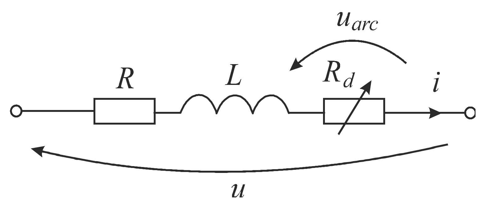
2. Mathematical Model of an Electric Branch with an Electrical Arc

In accordance with the main provisions of the method of average voltages in numerical integration step [23], the electric branch with inductance, active resistance and arc (Figure 1) is described by the following equation:

$$\frac{1}{\Delta t}{\displaystyle \underset{t_0}{\overset{t_0+\Delta t}{\int }}\left(u-u_R-u_L-u_{arc}(i)\right)dt}=0,$$

(1)

where u_R, u_L, u_arc—instantaneous values of voltage on active resistance, voltage on inductance, arc voltage, respectively; u—voltage applied to the branch; t₀—is the start time of integration step, Δt—is the numerical integration step.

The instantaneous values of voltages on the active resistance and on the arc are represented by the formulas:

$$u_R=u_{R0}+\Delta u_R, u_{arc}=u_{arc0}+\Delta u_{arc},$$

(2)

where u_R0, u_arc0—voltage values at the start of the step; Δu_R, Δu_arc—voltage gains at the step of numerical integration.

The voltage increments at the step of numerical integration are determined using the Taylor series:

$$\Delta u_R={\displaystyle \sum _{k=1}^m\frac{d^{\left(k\right)}{u}_{R0}}{d{t}^{\left(k\right)}}\cdot \frac{{\left(t-t_0\right)}^k}{k!}}, \Delta u_{arc}={\displaystyle \sum _{k=1}^m\frac{d^{\left(k\right)}{u}_{arc0}}{d{t}^{\left(k\right)}}\cdot \frac{{\left(t-t_0\right)}^k}{k!}}$$

(3)

where $\frac{d^{\left(k\right)}{u}_{R0}}{d{t}^{\left(k\right)}}$, $\frac{d^{\left(k\right)}{u}_{arc0}}{d{t}^{\left(k\right)}}$—k-th voltage derivatives on the active resistance and on the arc at the beginning of the step; m—is the number of derivatives taken into account (method order).

Taking into account the dependences between voltage and current for the active resistance of the circuit R and for the arc, respectively: $u_R\left(t\right)=Ri\left(t\right)$, $u_{arc}\left(t\right)=f\left(i\right)$, we obtain expressions for increments (4) and (5):

$$\Delta u_R={\displaystyle \sum _{k=1}^{m}R\frac{d^{\left(k\right)}{i}_0}{d{t}^{\left(k\right)}}\cdot \frac{{\left(t-t_0\right)}^k}{k!}}$$

(4)

$$\Delta u_{arc}={\displaystyle \sum _{k=1}^m\frac{d^{\left(k\right)}{u}_{arc0}}{d{i}^{\left(k\right)}}\frac{d^{\left(k\right)}{i}_0}{d{t}^{\left(k\right)}}\cdot \frac{{\left(t-t_0\right)}^k}{k!}}$$

(5)

For the 1st order method:

$$\Delta u_R=R\frac{d{i}_0}{dt}\Delta t, \Delta u_{arc}=\frac{d{u}_{arc0}}{di}\frac{d{i}_0}{dt}\Delta t=R_{d0}\frac{d{i}_0}{dt}\Delta t$$

(6)

where $R_d=\frac{d{u}_{arc}}{di}$—dynamic arc resistance (determined on the basis of instantaneous values of arc voltage u_arc and current (i); $R_{d0}$—dynamic arc resistance at the beginning of the step. Note that the dynamic resistance of the arc depends on the current of the arc and the length of the arc and is determined at each step.

Taking into account (2), (6) and the equation for the voltage on the inductance (the value of the inductance L is constant) $u_L(t)=L\frac{di(t)}{dt}$ from Equation (1) we obtain for the method of the 1st order:

$$U-u_{R0}-u_{arc0}-\left(\frac{R+R_{d0}}{2}+\frac{L}{\Delta t}\right)\left(i_1-i_0\right)=0$$

(7)

where i₀—current of circuit at the beginning of the integration step, i₁—is the current at the end of the integration step, $U=\frac{1}{\Delta t}{\displaystyle \underset{t_0}{\overset{t_0+\Delta t}{\int }}udt}$—the average value of the voltage applied to the circuit at the numerical integration step.

From Equation (7) we obtain the expression for determining the current of the branch at the end of the step:

$$i_1=i_0+{\left(\frac{R+R_{d0}}{2}+\frac{L}{\Delta t}\right)}^{-1}\left(U-R{i}_0-u_{arc0}\right).$$

(8)

The effective value of the arc voltage at each step of integration is calculated by the following formula:

$$u_{arc1}=u_{arc0}+R_d\Delta i,$$

(9)

where $\Delta i=i_1-i_0$—the increase in arc current on the step.

For the method of average voltages integration step of the 2nd order, the equations of voltage increments at the active resistance and at the arc will look like:

$$\Delta u_R=R\frac{d{i}_0}{dt}\Delta t+R\frac{d^2{i}_0}{d{t}^2}\frac{\Delta t^2}{2},$$

(10)

$$\Delta u_{arc}=\frac{d{u}_{arc0}}{di}\frac{d{i}_0}{dt}\Delta t+\frac{d^2{u}_{arc0}}{d{i}^2}\frac{d^2{i}_0}{d{t}^2}\frac{\Delta t^2}{2}=R_{d0}\frac{d{i}_0}{dt}\Delta t+\frac{d{R}_d}{di}\frac{d^2{i}_0}{d{t}^2}\frac{\Delta t^2}{2},$$

(11)

In this case, from Equations (1), (2), (10) and (11) we obtain:

$$U-R{i}_0-u_{arc0}+\left(\frac{R+R_{d0}}{3}+\frac{L}{\Delta t}\right)i_0-\frac{\Delta t}{6}(R+\frac{d{R}_{d0}}{di})\frac{d{i}_0}{dt}-\left(\frac{R+R_{d0}}{3}+\frac{L}{\Delta t}\right)i_1=0,$$

(12)

The expression for determining the circuit current at the end of the integration step will take the form:

$$i_1=i_0+{\left(\frac{R+R_{d0}}{3}+\frac{L}{\Delta t}\right)}^{-1}\left(U-R{i}_0-u_{arc0}\right)-\frac{\Delta t}{6}(R+\frac{d{R}_{d0}}{di})\frac{d{i}_0}{dt},$$

(13)

3. Mathematical Model of Arc Space of Electrical Arc Furnace

According to the chosen approach to EAF modeling, the description of the arc space does not use the arc model in the form of a volt-ampere characteristic, but rather the change of the dynamic arc resistance, which depends on both the current and the arc length. We demonstrate the application of this approach on the example of EAF-200. Experimentally obtained averaged dynamic Volt-Ampere characteristics for such a furnace are shown in Figure 2.

The dynamic Volt-Ampere characteristic of the arc has different curves when the current decreases and increases, and is also asymmetric. Then, obtained on the basis of experimental dynamic Volt-Ampere characteristics of the arc, the dependences of the dynamic resistance of the arc $R_d\left(I_{arc}, l_{arc}\right)$ for different lines will have the form shown in Figure 3.

The kind of the Volt-Ampere characteristic, which corresponds to the current drop, for a single arc length can be successfully approximated as:

$$U_{arc}=A_0\cdot th\left(\beta \cdot I_{arc}\right) if l_{arc}=const,$$

(14)

where A₀ and β approximation coefficients.

Then the equation for determining the dynamic resistance R_d will look like:

$$R_d\left(I_{arc},\right)=A_0\cdot \beta \cdot \left(1-\left(th{\left(\beta \cdot I_{arc}\right)}^2\right)\right),$$

(15)

The change in dynamic resistance R_d obtained on the basis of experimental volt-ampere characteristics and its approximation by the equation for R_d(I_arc) when I_arc = 10 mm are given in Figure 4. Significant deviations observed in the regions of large currents are explained primarily by the shortcomings of the construction of the Volt-Ampere characteristic based on experimental data.

In the case of current increasing, the approximation formula is much more complex. Analysis of different models of the current-voltage characteristic curves approximation is given in [22]. We need the derivative of a rather complex model to approximate the arc volt-ampere characteristic to determine R_d. In our opinion, it is more appropriate to approximate the dependence R_d(I_arc) for a given arc length.

If we ignore the asymmetry, the obtained dependence of the change in dynamic resistance resembles the curve obtained when using the Mexican hat wavelet [29].

The equation for approximating the characteristic R_d(I_arc) for a given arc length can be described as:

$$R_d\left({\mathrm{I}}_{arc}\right)=\frac{0.4337}{\sqrt{\sigma }}\cdot a_{11}\cdot \left(1-{\left(\frac{I_{arc}}{\sigma \cdot a_{21}}\right)}^2\right)\cdot exp\left(-a_{31}\cdot {\left(\frac{I_{arc}}{\sigma }\right)}^{2\cdot a_{41}}\right)$$

(16)

where $a_{11}, a_{21}, a_{31}, a_{41}$ are required parameters.

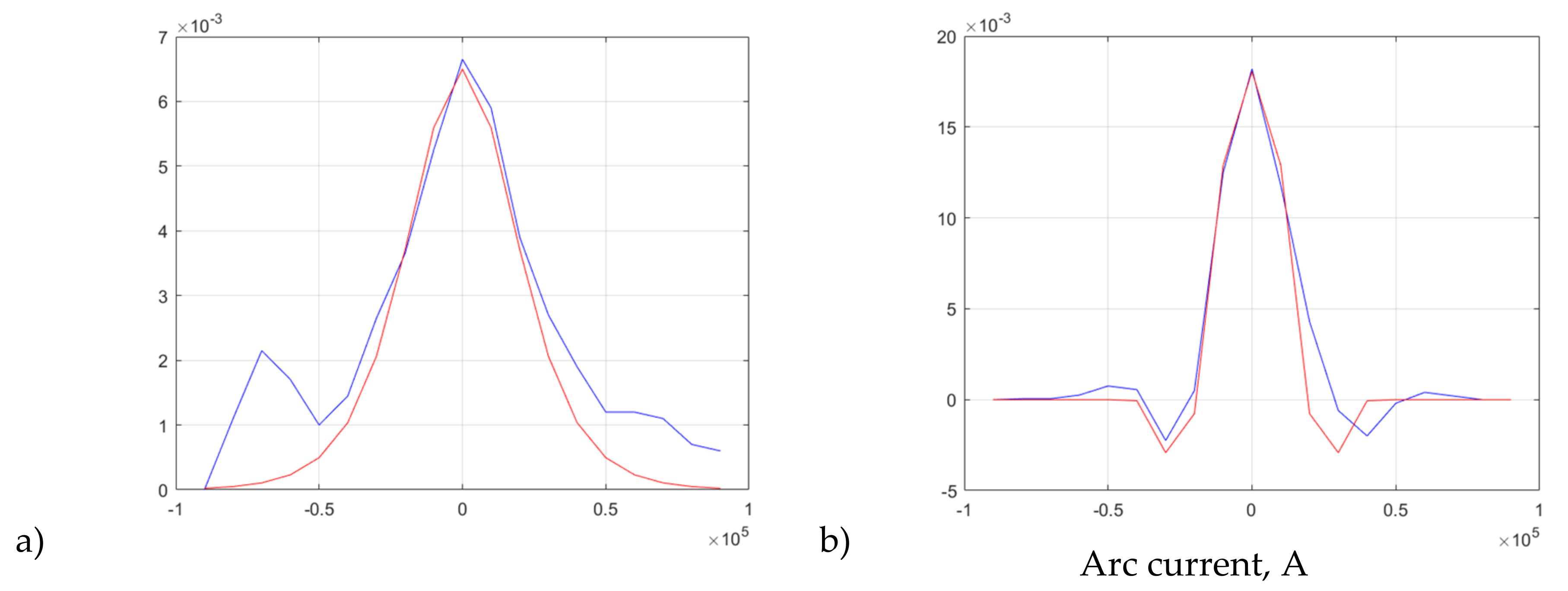
The change in dynamic resistance R_d obtained on the basis of experimental volt-ampere characteristics and its approximation using (16) for I_arc = 10 mm at $a_{11}=9.4, a_{21}=0.38, a_{31}=18, a_{41}=2$ and $\sigma =\mathrm{51,000}$ are given in Figure 4b. To take into account the asymmetry of the Volt-Ampere characteristic of the arc, it is necessary to separately determine the coefficients $a_{11}, a_{21}, a_{31}, a_{41}$ and $\sigma$ at I_arc < 0 and I_arc ≥ 0.

Approximating the obtained values of the coefficients at different arc lengths using polynomials of the appropriate order, we obtain the following equation to determine the dynamic resistance as a function of current and arc length:

if $I_{arc}\cdot \frac{d{I}_{arc}}{dt}>0$ then:

$$R_d\left(I_{arc}, l_{arc}\right)=\frac{0.4337}{\sqrt{\sigma \left( l_{arc}\right)}}\cdot a_{11}\left( l_{arc}\right)\cdot \left(1-{\left(\frac{I_{arc}}{\sigma \left( l_{arc}\right)\cdot a_{21}\left( l_{arc}\right)}\right)}^2\right)exp\left(-a_{31}\left( l_{arc}\right)\cdot {\left(\frac{I_{arc}}{\sigma \left( l_{arc}\right)}\right)}^{2\cdot a_{41}\left( l_{arc}\right)}\right)$$

if $I_{arc}\cdot \frac{d{I}_{arc}}{dt}<0$ then:

$$R_d\left(I_{arc},l_{arc}\right)=a_0\left( l_{arc}\right)\cdot \left(1-\left(th{\left(\frac{I_{arc}}{\sigma \left( l_{arc}\right)\cdot 0.5}\right)}^2\right)\right)$$

where:

$$a_{11}\left( l_{arc}\right)=0.9658\cdot l_{arc}-0.1282;$$

$$a_{21}\left( l_{arc}\right)=2.0477\cdot {10}^{-5}\cdot l_{arc}{}^3-0.0005\cdot l_{arc}{}^2+0.0019\cdot l_{arc}+0.3992;$$

$$a_{31}\left( l_{arc}\right)=-0.0026\cdot l_{arc}{}^3+0.0939\cdot l_{arc}{}^2-0.3429\cdot l_{arc}+14.0293;$$

$$a_{41}\left( l_{arc}\right)=2;$$

$$\sigma \left( l_{arc}\right)=\left(0.0093\cdot l_{arc}{}^2-0.4513\cdot l_{arc}+9.2986\right)\cdot \mathrm{10,000};$$

$$a_0\left( l_{arc}\right)=\left(0.0004\cdot l_{arc}{}^4-0.0124\cdot l_{arc}{}^3+0.1468\cdot l_{arc}{}^2+0.0081\cdot l_{arc}+0.1418\right)/1000.$$

The obtained dependences of the change of dynamic resistance R_d (I_arc, l_arc) when applying the found approximation functions are given in Figure 5.

Comparison of the obtained dependences of the dynamic resistance change with the ones shown in Figure 3 dependences allows us to state, that the dependences obtained on the basis approximation functions application of reproduce the nature of the change in dynamic resistance with a change in current and arc length.

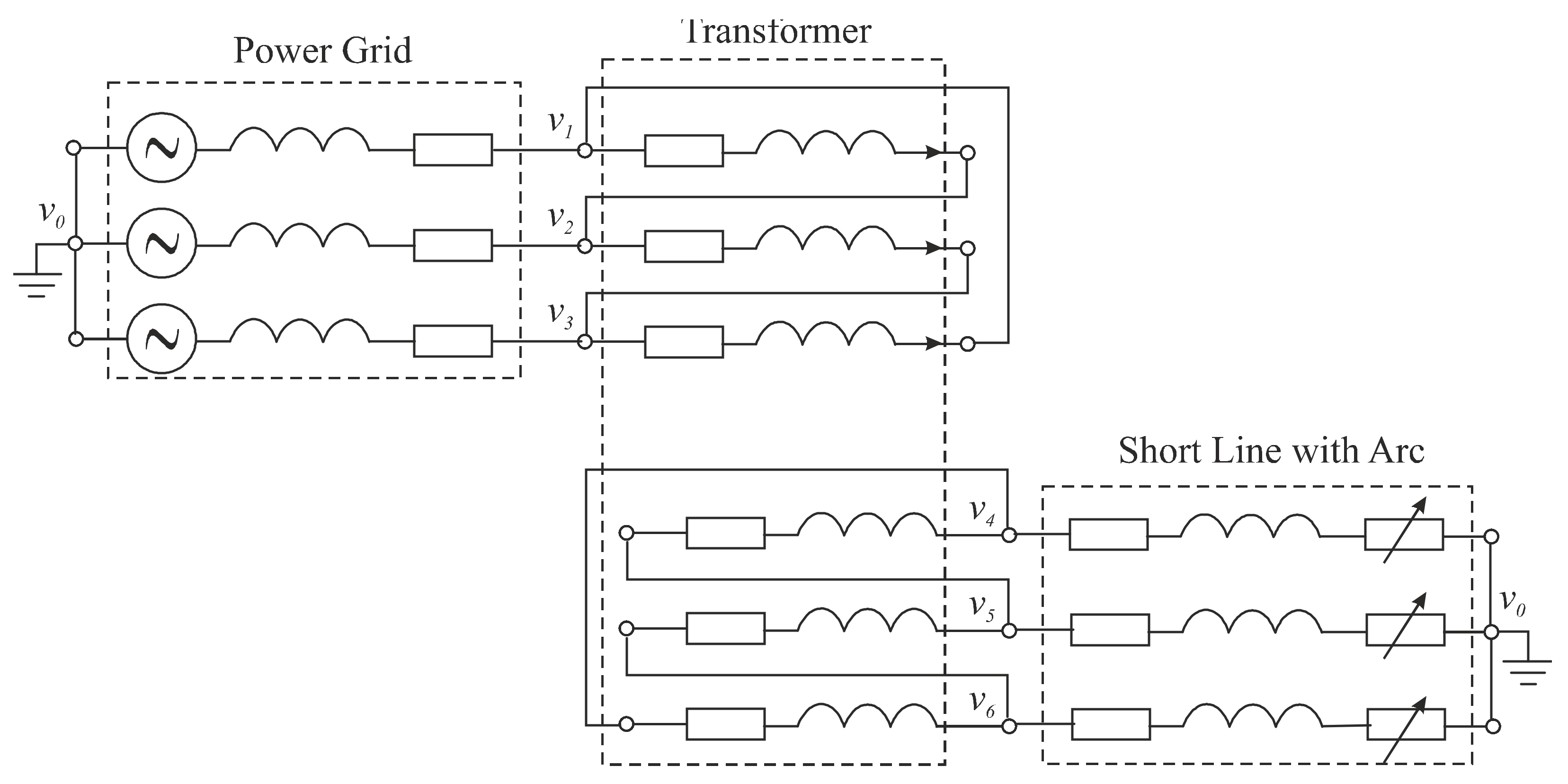
4. Mathematical Models of Power System Elements of Electrical Arc Furnace

According to the approach described in [23,24], the calculation scheme of a three-phase short network with a furnace space (arc) is presented in the form of a six-pole (Figure 6).

Such a multipole is described by a vector Equation (17):

$${\overrightarrow{i}}_{SL}+G_{SL}\frac{1}{\Delta t}{\displaystyle \underset{t_0}{\overset{t_0+\Delta t}{\int }}{\overrightarrow{v}}_{SL}dt}+{\overrightarrow{C}}_{SL}=0$$

(17)

which connects the currents of the outer branches of the multipole ${\overrightarrow{i}}_{SL}={\left(i_{SLA1},i_{SLB1},i_{SLC1},i_{SLA2},i_{SLB2},i_{SLC2}\right)}^T$ with the average values of the potentials of the external poles at the step of numerical integration $\frac{1}{\Delta t}{\displaystyle \underset{t_0}{\overset{t_0+\Delta t}{\int }}{\overrightarrow{v}}_{SL}dt}$, ${\overrightarrow{v}}_{SL}=\left(\begin{array}{c}{\overrightarrow{v}}_{SL1}\\ {\overrightarrow{v}}_{SL2}\end{array}\right)$, ${\overrightarrow{v}}_{SL1}={\left(v_{SLA1},v_{SLB1},v_{SLC1}\right)}^T$, ${\overrightarrow{v}}_{SL2}={\left(v_{SLA2},v_{SLB2},v_{SLC2}\right)}^T$.

Equation (17) is obtained from Equation (8), taking into account that the vector of the average values of the applied voltage at the integration step is equal to:

$${\overrightarrow{U}}_{SL}=\frac{1}{\Delta t}{\displaystyle \underset{t_0}{\overset{t_0+\Delta t}{\int }}{\overrightarrow{v}}_{SL1}dt}-\frac{1}{\Delta t}{\displaystyle \underset{t_0}{\overset{t_0+\Delta t}{\int }}{\overrightarrow{v}}_{SL2}dt}.$$

The coefficients of Equation (17) are defined as a matrix:

$$\begin{gathered} G_{SL}=\left[\begin{array}{cccccc}R{\ast }_{SLA}^{-1}& 0& 0& -R{\ast }_{LA}^{-1}& 0& 0\\ 0& R{\ast }_{LB}^{-1}& 0& 0& -R{\ast }_{LB}^{-1}& 0\\ 0& 0& R{\ast }_{LC}^{-1}& 0& 0& -R{\ast }_{LC}^{-1}\\ -R{\ast }_{LA}^{-1}& 0& 0& R{\ast }_{LA}^{-1}& 0& 0\\ 0& -R{\ast }_{LB}^{-1}& 0& 0& R{\ast }_{LB}^{-1}& 0\\ 0& 0& -R{\ast }_{LC}^{-1}& 0& 0& R{\ast }_{LC}^{-1}\end{array}\right] \\ {\overrightarrow{C}}_{SL}=\left[\begin{array}{c}-R{\ast }_{SLA}^{-1}\left(R_{SLA}{i}_{SLA0}+u_{arcA0}\right)+i_{SLA0}\\ -R{\ast }_{SLB}^{-1}\left(R_{SLB}{i}_{SLB0}+u_{arcB0}\right)+i_{SLB0}\\ -R{\ast }_{SLC}^{-1}\left(R_{SLC}{i}_{SLC0}+u_{arcC0}\right)+i_{SLC0}\\ R{\ast }_{SLA}^{-1}\left(R_{SLA}{i}_{SLA0}-u_{arcA0}\right)-i_{SLA0}\\ R{\ast }_{SLB}^{-1}\left(R_{SLB}{i}_{SLB0}-u_{arcB0}\right)-i_{SLB0}\\ R{\ast }_{SLC}^{-1}\left(R_{SLC}{i}_{SLC0}-u_{arcC0}\right)-i_{SLC0}\end{array}\right] \end{gathered}$$

where $R{\ast }_{SLA}=\frac{R_{SLA}+R_{\partial A0}}{2}+\frac{L_{SLA}}{\Delta t}$, $R{\ast }_{SLB}=\frac{R_{SLB}+R_{\partial B0}}{2}+\frac{L_{SLB}}{\Delta t}$, $R{\ast }_{SLC}=\frac{R_{SLC}+R_{\partial C0}}{2}+\frac{L_{SLC}}{\Delta t}$—step phases resistances, $i_{SLA}=-i_{SLA1}=i_{SLA2}$, $i_{SLB}=-i_{SLB1}=i_{SLB2}$, $i_{SLC}=-i_{SLC1}=i_{SLC2}$—phase currents.

The three-phase transformer is represented by a 12-pole (see Figure 7), the outer circuits of which are the winding outputs

Using an approach similar to the network model with an arc had need applied, we obtain the vector equation of a three-phase transformer:

$${\overrightarrow{i}}_{TR}+G_{TR}\frac{1}{\Delta t}{\displaystyle \underset{t_0}{\overset{t_0+\Delta t}{\int }}{\overrightarrow{v}}_{TR}dt}+{\overrightarrow{C}}_{TR}=0$$

(18)

where ${\overrightarrow{i}}_{TR}={\left(-{\overrightarrow{i}}_{tr},{\overrightarrow{i}}_{tr}\right)}^T$– vector of external branches currents; ${\overrightarrow{i}}_{tr}={\left({\mathrm{i}}_{TA},i_{TB},i_{TC},i_{T\mathrm{a}},i_{Tb},i_{Tc}\right)}^T$—vector of primary and secondary transformer windings currents; ${\overrightarrow{v}}_{TR}={\left(v_{TA1},v_{TB1},v_{TC1},v_{T\mathrm{a}1},v_{Tb1},v_{Tc1},v_{TA2},v_{TB2},v_{TC2},v_{T\mathrm{a}2},v_{Tb2},v_{Tc2}\right)}^T$—vector of external poles potentials.

The coefficients of Equation (18) are defined as follows:

$${\stackrel{⌣}{G}}_T=\left[\begin{array}{cc}R{\ast }_{TR}^{-1}& -R{\ast }_{TR}^{-1}\\ -R{\ast }_{TR}^{-1}& R{\ast }_{TR}^{-1}\end{array}\right],{\overrightarrow{C}}_{TR}=\left[\begin{array}{c}-R{\ast }_{TR}^{-1}\left(R_{TR}{\overrightarrow{i}}_{tr0}\right)+{\overrightarrow{i}}_{tr0}\\ R{\ast }_{TR}^{-1}\left(R_{TR}{\overrightarrow{i}}_{tr0}\right)-{\overrightarrow{i}}_{tr0}\end{array}\right]$$

where $R{\ast }_{TR}^{}=\frac{R_{TR}^{}}{2}+\frac{L_{TR}}{\Delta t}$—matrix of step resistances of the transformer; $R_{TR}=diag\left(R_{TA},R_{TB},R_{TC},R_{T\mathrm{a}},R_{Tb},R_{Tc}\right)$—matrix of windings active resistances; $L_{TR}$—matrix of self- and mutual- inductances of windings:

$$L_{TR}=\left[\begin{array}{cccccc}{L}_{AA}& L_{AB}& L_{AC}& L_{Aa}& L_{Ab}& L_{Ac}\\ L_{BA}& L_{BB}& L_{BC}& L_{Ba}& L_{Bb}& L_{Bc}\\ L_{CA}& L_{CB}& L_{CC}& L_{Ca}& L_{Cb}& L_{Cc}\\ L_{aA}& L_{aB}& L_{aC}& L_{aa}& L_{ab}& L_{ac}\\ L_{bA}& L_{bB}& L_{bC}& L_{ba}& L_{bb}& L_{bc}\\ L_{cA}& L_{cB}& L_{cC}& L_{ca}& L_{cb}& L_{cc}\end{array}\right]$$

A three-phase network with a choke is represented by a six-pole (Figure 8):

Similarly, applying of AVIS method into the electrical circuit of a three-phase network with a choke, we obtain the Equation (19):

$$\begin{gathered} i_{NA1}=i_{NA0}+{\left(\frac{R_{NA}}{2}+\frac{L_{NA}}{\Delta t}\right)}^{-1}\left(U_{NA}+E_{NA}-R_{NA}{i}_{NA0}\right) \\ {i}_{NB1}=i_{NB0}+{\left(\frac{R_{NB}}{2}+\frac{L_{NB}}{\Delta t}\right)}^{-1}\left(U_{NB}+E_{NB}-R_{NA}{i}_{NB0}\right) \\ {i}_{NC1}=i_{NC0}+{\left(\frac{R_{NC}}{2}+\frac{L_{NC}}{\Delta t}\right)}^{-1}\left(U_{NC}+E_{NC}-R_{NA}{i}_{NC0}\right) \end{gathered}$$

(19)

where R_NA, R_NB, R_NC—resistance of phases; L_NA, L_NB, L_NC inductance of phases in choke; $U_{NA}=\frac{1}{\Delta t}{\displaystyle \underset{t_0}{\overset{t_0+\Delta t}{\int }}{u}_{NA}dt}$, $U_{NB}=\frac{1}{\Delta t}{\displaystyle \underset{t_0}{\overset{t_0+\Delta t}{\int }}{u}_{NB}dt}$, $U_{NC}=\frac{1}{\Delta t}{\displaystyle \underset{t_0}{\overset{t_0+\Delta t}{\int }}{u}_{NC}dt}$—average of a branch voltages at the integration step; $E_{NA}=\frac{1}{\Delta t}{\displaystyle \underset{t_0}{\overset{t_0+\Delta t}{\int }}{e}_{NA}dt}$, $E_{NB}=\frac{1}{\Delta t}{\displaystyle \underset{t_0}{\overset{t_0+\Delta t}{\int }}{e}_{NB}dt}$, $E_{NC}=\frac{1}{\Delta t}{\displaystyle \underset{t_0}{\overset{t_0+\Delta t}{\int }}{e}_{NC}dt}$—average values of EMF in integration step.

Based on the system of Equation (19), the vector equation of a three-phase network with a choke as a six-pole can be written as:

$${\overrightarrow{i}}_N+G_N\frac{1}{\Delta t}{\displaystyle \underset{t_0}{\overset{t_0+\Delta t}{\int }}{\overrightarrow{v}}_{N}dt}+{\overrightarrow{C}}_N=0$$

(20)

where ${\overrightarrow{i}}_N={\left(i_{NA},i_{NB},i_{NC},-i_{NA},-i_{NB},-i_{NC}\right)}^T$—vector of currents of outer brunches, ${\overrightarrow{v}}_N={\left(v_{NA1},v_{NB1},v_{NC1},v_{NA2},v_{NB2},v_{NC2}\right)}^T$—vector of potentials of external poles:

$$\begin{gathered} G_N=\left[\begin{array}{cccccc}R{\ast }_{NA}^{-1}& 0& 0& -R{\ast }_{NA}^{-1}& 0& 0\\ 0& R{\ast }_{NB}^{-1}& 0& 0& -R{\ast }_{NB}^{-1}& 0\\ 0& 0& R{\ast }_{NC}^{-1}& 0& 0& -R{\ast }_{NC}^{-1}\\ -R{\ast }_{NA}^{-1}& 0& 0& R{\ast }_{NA}^{-1}& 0& 0\\ 0& -R{\ast }_{NB}^{-1}& 0& 0& R{\ast }_{NB}^{-1}& 0\\ 0& 0& -R{\ast }_{NC}^{-1}& 0& 0& R{\ast }_{NC}^{-1}\end{array}\right], \\ {\overrightarrow{C}}_{SL}=\left[\begin{array}{c}-R{\ast }_{NA}^{-1}\left(R_{NA}{i}_{NA0}\right)+i_{NA0}\\ -R{\ast }_{NB}^{-1}\left(R_{NB}{i}_{NB0}\right)+i_{NB0}\\ -R{\ast }_{NC}^{-1}\left(R_{NC}{i}_{NC0}\right)+i_{NC0}\\ R{\ast }_{NA}^{-1}\left(R_{NA}{i}_{NA0}\right)-i_{NA0}\\ R{\ast }_{NB}^{-1}\left(R_{NB}{i}_{NB0}\right)-i_{NB0}\\ R{\ast }_{NC}^{-1}\left(R_{NC}{i}_{NC0}\right)-i_{NC0}\end{array}\right] \end{gathered}$$

where $R{\ast }_{NA}=\frac{R_{NA}}{2}+\frac{L_{NA}}{\Delta t}$, $R{\ast }_{NB}=\frac{R_{NB}}{2}+\frac{L_{NB}}{\Delta t}$, $R{\ast }_{NC}=\frac{R_{NC}}{2}+\frac{L_{NC}}{\Delta t}$—step resistances of network with choke.

5. Simulation Model and Calculation Algorithm of Power Supply System of Electrical Arc Furnace

The mathematical model of the arc power supply system is formed from the models of its separate multipole elements connected according to the calculation scheme shown in Figure 9.

The outer branches of the multipoles are interconnected at the nodes of the electrical circuit. The connection method is mathematically described by incidence matrices, which indicate with which independent nodes of the system the poles of the multipole element are connected. For schemes, which shown in Figure 9, the incidence matrices of elements are following: for a three-phase network with a choke ${\Pi }_N=\left[\begin{array}{cccccc}0& 0& 0& 1& 0& 0\\ 0& 0& 0& 0& 1& 0\\ 0& 0& 0& 0& 0& 1\\ 0& 0& 0& 0& 0& 0\\ 0& 0& 0& 0& 0& 0\\ 0& 0& 0& 0& 0& 0\end{array}\right]$, ${\Pi }_{TR}=\left[\begin{array}{cccccccccccc}1& 0& 0& 0& 0& 0& 0& 0& 1& 0& 0& 0\\ 0& 1& 0& 0& 0& 0& 1& 0& 0& 0& 0& 0\\ 0& 0& 1& 0& 0& 0& 0& 1& 0& 0& 0& 0\\ 0& 0& 0& 0& 0& 1& 0& 0& 0& 1& 0& 0\\ 0& 0& 0& 1& 0& 0& 0& 0& 0& 0& 1& 0\\ 0& 0& 0& 0& 1& 0& 0& 0& 0& 0& 0& 1\end{array}\right]$—for transformer, ${\Pi }_{S\mathrm{L}}=\left[\begin{array}{cccccc}0& 0& 0& 0& 0& 0\\ 0& 0& 0& 0& 0& 0\\ 0& 0& 0& 0& 0& 0\\ 1& 0& 0& 0& 0& 0\\ 0& 1& 0& 0& 0& 0\\ 0& 0& 1& 0& 0& 0\end{array}\right]$—for the short network with furnace space.

According to the algorithm described in [24], the average in integration step values of the potentials of the independent nodes in system ${\overrightarrow{V}}_S=\frac{1}{\Delta t}{\displaystyle \underset{t_0}{\overset{t_0+\Delta t}{\int }}{\overrightarrow{v}}_{S}dt}$, ${\overrightarrow{v}}_S={\left(v_1,v_2,v_3,v_4,v_5,v_6\right)}^T$ we can find from Equation (21):

$$G_S\frac{1}{\Delta t}{\displaystyle \underset{t_0}{\overset{t_0+\Delta t}{\int }}{\overrightarrow{v}}_{S}dt}+{\overrightarrow{C}}_S=0,$$

(21)

matrices of coefficients which are determined on the basis of coefficients of Equations (17), (18) and (20) and incidence matrices as:

$$G_S={\Pi }_N{G}_N{\Pi }_N^T+{\Pi }_{TR}{G}_{TR}{\Pi }_{TR}^T+{\Pi }_{SL}{G}_{SL}{\Pi }_{SL}^T, {\overrightarrow{C}}_S={\Pi }_N{\overrightarrow{C}}_N+{\Pi }_{TR}{\overrightarrow{C}}_{TR}+{\Pi }_{SL}{\overrightarrow{C}}_{SL}.$$

The system (21) is solved at each integration step with respect to the vector of averages in step values of potentials of the independent nodes in the system, then determine the averages value of the pole potentials of each element can be rewriten as:

for three-phase network with a choke ${\overrightarrow{V}}_N=\frac{1}{\Delta t}{\displaystyle \underset{t_0}{\overset{t_0+\Delta t}{\int }}{\overrightarrow{v}}_{N}dt}={\Pi }_N^T\cdot {\overrightarrow{V}}_S={\Pi }_N^T\cdot \left(\frac{1}{\Delta t}{\displaystyle \underset{t_0}{\overset{t_0+\Delta t}{\int }}{\overrightarrow{v}}_{S}dt}\right)$, for transformer ${\overrightarrow{V}}_{TR}=\frac{1}{\Delta t}{\displaystyle \underset{t_0}{\overset{t_0+\Delta t}{\int }}{\overrightarrow{v}}_{TR}dt}={\Pi }_{TR}^T\cdot {\overrightarrow{V}}_S={\Pi }_{TR}^T\cdot \left(\frac{1}{\Delta t}{\displaystyle \underset{t_0}{\overset{t_0+\Delta t}{\int }}{\overrightarrow{v}}_{S}dt}\right)$ and for the short network with furnace space ${\overrightarrow{V}}_{SL}=\frac{1}{\Delta t}{\displaystyle \underset{t_0}{\overset{t_0+\Delta t}{\int }}{\overrightarrow{v}}_{SL}dt}={\Pi }_{SL}^T\cdot {\overrightarrow{V}}_S={\Pi }_{SL}^T\cdot \left(\frac{1}{\Delta t}{\displaystyle \underset{t_0}{\overset{t_0+\Delta t}{\int }}{\overrightarrow{v}}_{S}dt}\right)$.

After determining the average in the step values of the pole potentials of each element by Equations (17), (18) and (20), can be determined the vectors of the currents of the outer branches:

$$\begin{gathered} {\overrightarrow{i}}_N=-G_N\frac{1}{\Delta t}{\displaystyle \underset{t_0}{\overset{t_0+\Delta t}{\int }}{\overrightarrow{v}}_{N}dt}-{\overrightarrow{C}}_N, \\ {\overrightarrow{i}}_{TR}=-G_{TR}\frac{1}{\Delta t}{\displaystyle \underset{t_0}{\overset{t_0+\Delta t}{\int }}{\overrightarrow{v}}_{TR}dt}-{\overrightarrow{C}}_{TR}, \\ {\overrightarrow{i}}_{SL}=-G_{SL}\frac{1}{\Delta t}{\displaystyle \underset{t_0}{\overset{t_0+\Delta t}{\int }}{\overrightarrow{v}}_{SL}dt}-{\overrightarrow{C}}_{SL}. \end{gathered}$$

The calculation algorithm, which was described above, starting from finding of coefficients of vector equations of elements-multipoles (17), (18), (20) and finishing with definition of vectors of currents of external branches is cyclic.

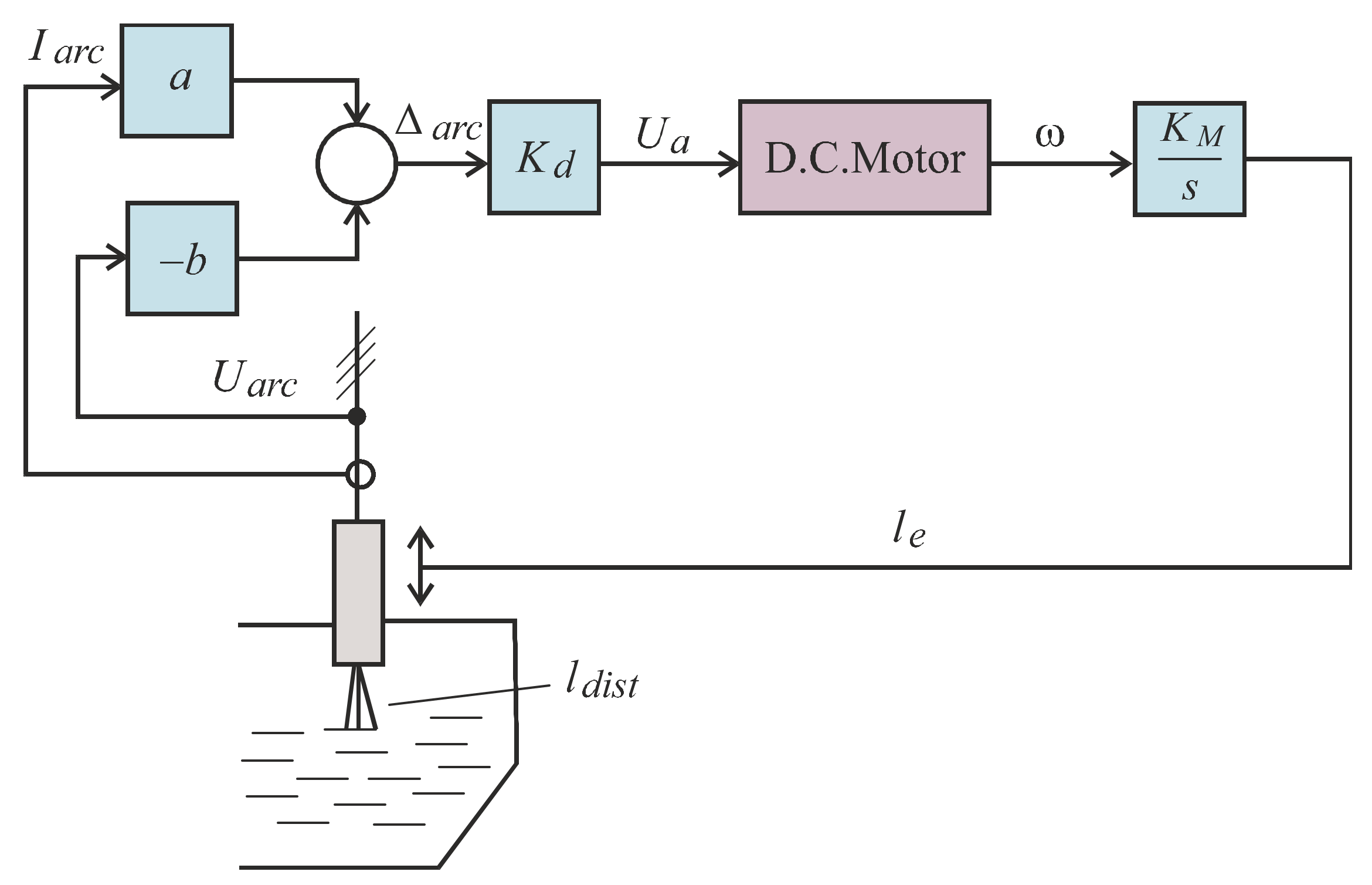
6. Mathematical Model of the Electrode Movement System

The electric drive of the electrode movement system (see Figure 10) uses a DC motor for each phase. Its supply voltage is formed by a thyristor converter based on the mismatch signal Δ_arc, which is defined by Equation (22):

Δ _arc = aI_arc − bU_arc

(22)

where I_arc, U_arc—current values of arc current and voltage; a, b—proportionality factros (setpoint).

The value of the electrode movement is defined as:

$$l_e=K_M{\displaystyle \underset{t_0}{\overset{t_0+\Delta t}{\int }}\omega dt}$$

(23)

where K_M—the transmission coefficient of the mechanical system; J—the moment of inertia; ω—the angular speed of the motor.

The length of the arc l_arc is determined by the sum of the displacement of the electrode le and the displacement of the charge in the melt process l_dist, which are perturbations in the furnace space $l_{arc}=l_e\pm l_{dist}$. It should be noted that l_dist changes randomly and the task of the automated control system (ACS) is to ensure that these perturbations work out.

Mathematical description of the DC motor by the method of medium voltages in the integration step of the first order is described in [30] and has the form:

$$i_{a1}=\left(U_a-K_{\mathsf{\Phi }}{\omega }_0-R_a{i}_{a0}+\left(\frac{R_a}{2}+\frac{L_a}{\Delta t}-\frac{K_{\mathsf{\Phi }}^2\Delta t}{3J}\right)i_{a0}\right)\times {\left(\frac{R_a}{2}+\frac{L_a}{\Delta t}-\frac{K_{\mathsf{\Phi }}^2\Delta t}{6J}\right)}^{-1}$$

(24)

$${\omega }_1={\omega }_0+\frac{K_{\mathsf{\Phi }}^{}\Delta t}{2J}\left(i_{a0}+i_{a1}\right)$$

(25)

where i_a0, i_a1—the armature current of the motor at the beginning and end of the integration step; ω₀, ω₁—angular rotation speed at the beginning and end of the integration step; U_a—supply voltage; R_a—the active resistance of the armature winding; L_a—inductance of the armature winding; K_Φ—design factor; J—moment of inertia. In the described model, the value of the static torque of the motor, which is small compared to the dynamic torque, is neglected.

The magnitude of the electrodes movement is defined by the following equation:

$$l_{e1}=l_{e0}+\frac{K_M^{}\Delta t}{2}\left({\omega }_0+{\omega }_1\right)$$

(26)

7. The Results of Process Investigation

The results of calculation of steady symmetrical modes in the arc power supply system for different values of arc length: 2 mm (in Figure 11) and 20 mm (in Figure 12) are given in Figure 11 and Figure 12. As shown by the results of studies, increasing the length of the arc leads to an increase in the dynamic resistance of the arc, an increase in arc voltage and a decrease in current in the supply circuit.

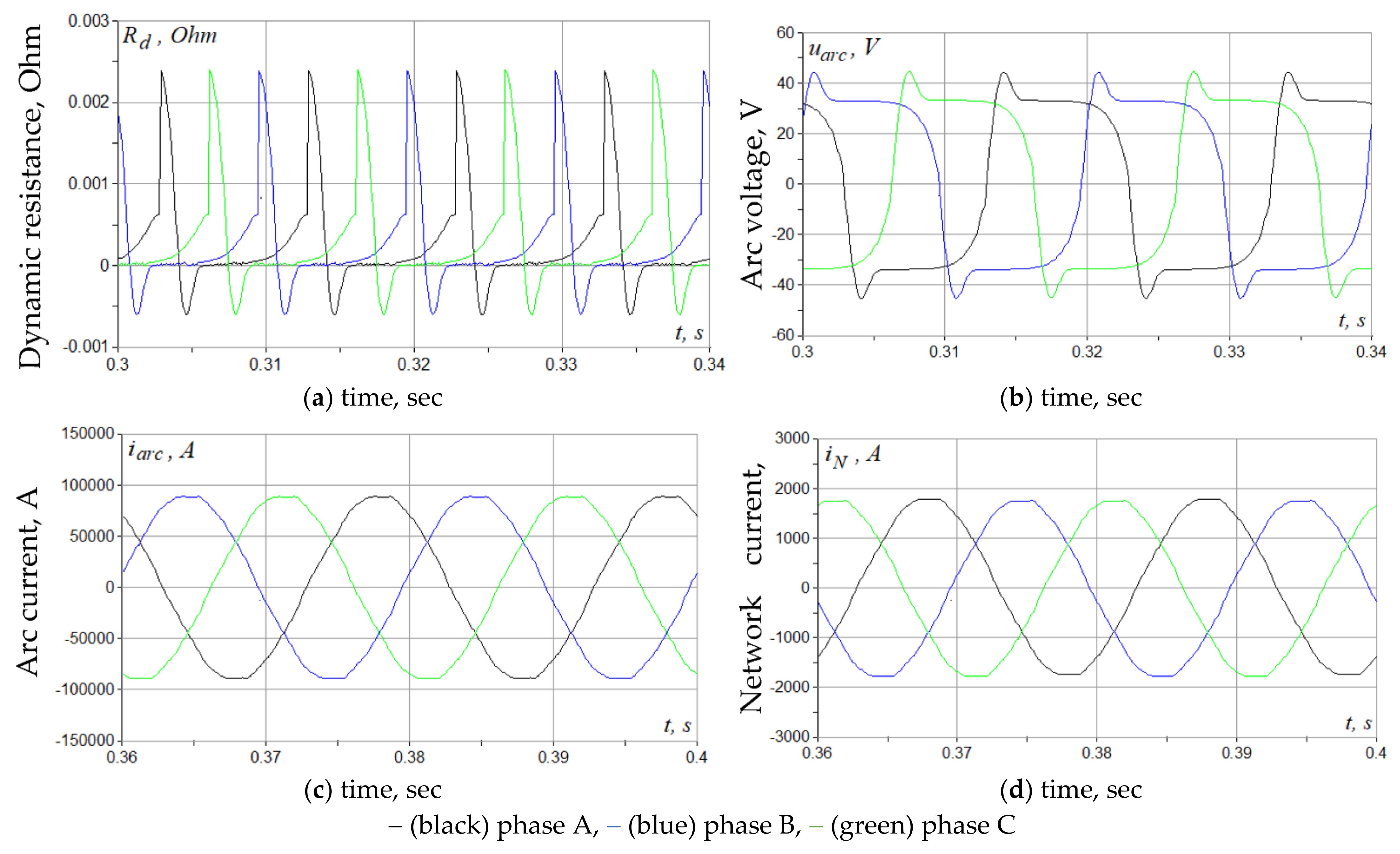
Increasing the length of the arc also leads to a deterioration of the shape of the current in the arc supply circuit and the shape of the current (Figure 12c) consumed from the mains (Figure 12d). The results of calculation of the steady asymmetric mode in the power supply system of arcs for different values of arc length in phases: phase A—2 mm, phase B—8 mm, phase C—20 mm are shown in Figure 13.

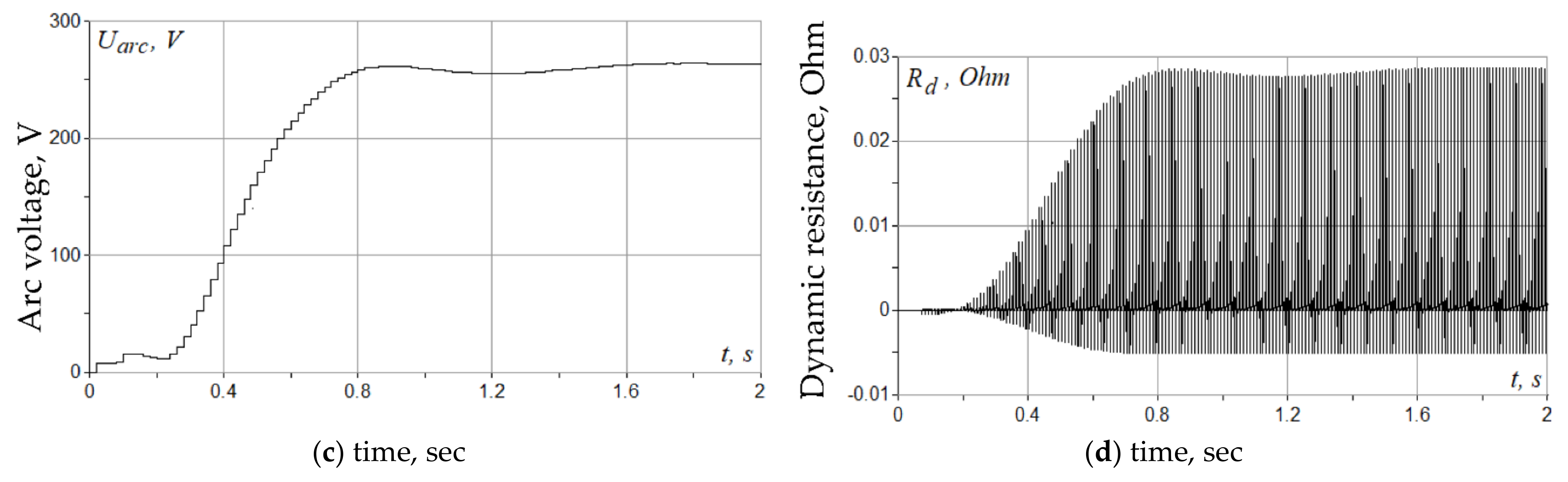
In Figure 14 are shown the results of the calculation of the transient mode of arc ignition and the output to the operating mode, which is determined by the ACS for the electrodes movement which described above (Figure 10). The electrode movement system provides the formation of the arc length for which the mismatch signal defined by expression (22) becomes equal to 0.

The nature of the change in the obtained dependences of current and arc voltage, current and voltage of the power supply network corresponds to the experimentally removed dependences given in the publications of other authors, in particular [18]. In addition, the models created on the basis of the proposed approach can function in combination with physical objects, which createsmodel predictive control.

The simulation results completely repeat the dependences obtained using the EAF model, in which the dynamic volt-ampere characteristics of the arc are tabulated and the 4th order Runge-Kutta method is used for calculations. However, the model proposed in this article has a higher (several times) calculation speed and numerical stability (the ability to perform calculations over long time intervals).The adequacy of the mentioned model of EAF with approximated volt-ampere characteristics of arcs was confirmed using the methods of statistical data analysis, in particular the method of one-way analysis of variance [31], which based on the following equation:

$$t=\frac{N-k}{k-1}\cdot \frac{{\displaystyle \sum _{i=1}^k{n}_i\cdot {\left({\overline{x}}_i-\overline{x}\right)}^2}}{{\displaystyle \sum _{i=1}^k{\displaystyle \sum _{j=1}^{n_i}{\left(x_{ij}-{\overline{x}}_i\right)}^2}}}$$

(27)

where $N={\displaystyle \sum _{i=1}^k{n}_i}$—input number; k—number of samples; n_i, i = 1, 2, …, k—number of i-th sample; ${\overline{x}}_i=\frac{1}{n_i}\cdot {\displaystyle \sum _{j=1}^{n_i}{x}_{ij}},i=1,2,\dots ,k$—average value of i-th sample; $\overline{x}=\frac{1}{N}{\displaystyle \sum _{i=1}^k{\displaystyle \sum _{j=1}^{n_i}{x}_{ij}}}$—summarized average value; M—factor of Barlett criteria [31].

$$\begin{array}{l}t=\frac{\ln 10}{c}\left[\left(N-k\right)\cdot \lg s^2-{\displaystyle \sum _{}^{}\left(n_i-1\right)\cdot \lg s_i^2}\right]\\ c=1+\frac{1}{3\cdot \left(k-1\right)}\cdot \left({\displaystyle \sum _{i=1}^k\frac{1}{n_i-1}-\frac{1}{N-k}}\right)\\ s^2=\frac{1}{N-k}\cdot {\displaystyle \sum _{}^{}\left(n_i-1\right)\cdot s_i^2}\end{array}$$

where $s_i^2=\frac{1}{n_i-1}\cdot {\displaystyle \sum _{j=1}^{n_i}{\left(x_{ij}-{\overline{x}}_i\right)}^2}$—variance of the i-th sample

These equations applying for data samples, which are shown in Figure 15 and Figure 16. These dependencies correspond to the modes of the beginning of melting and the mode of completion of melting of wells.

To obtain the results of mathematical modeling on the model of EAF, perturbations were applied, which in their spectral characteristics correspond to the perturbations acting in a real furnace at this stage of melting. In Figure 15a the scale for I 10 mm = 25,000 A, for time—10 mm = 0.2 s; in Figure 16–scale for I-axes—10 mm = 20,000 A, for time—10 mm = 0.2 s.

As can be seen from results in

Table 1. Statistical data analysis.

		Number of Samples	Average Value	Value of Criterion (14)	Dispersion	Value M Barlett Criterion
Melting start	experiment	301	44,580	2.93	1.876 × 108	1924
	model	919	45,860		1648 × 108
Valid criterion value				3.84		384
Copletion of wells melting	experiment	301	47,420	1.191	1037 × 108	3079
	model	6001	47,720		1205 × 108
Valid criterion value				3.84		384

, the values of the relevant criteria obtained for different modes of operation of the EAF are less than the corresponding tabular values taken for 5%—the level of significance, which allowed us to conclude that the created system model adequately reflects the processes taking place in a real life project.

It should be noted that the speed of the EAF model created using the method of medium voltage at the integration step and the use of dynamic arc resistance approximation is almost two orders of magnitude higher than the model with tabular volt-ampere characteristics and 4th order Runge-Kutta method, as well as the fact that the system retains numerical stability over long intervals of calculations.

In further research authors plan to analyze the influence of different control systems (single-circuit—when implementing different laws of electrode movement control and double-circuit—with additional high-speed inductor control circuit) on the characteristics of the power supply network, and to synthesize new, effective laws of arc electrode movement control of EAF using fractional and intelligent controllers for single- and double-circuit control systems.

8. Conclusions

Using the method of medium voltages at the step of numerical integration a mathematical model of the arc power system is developed. Such a model of the arc power system with electromechanical electrode movement system allows one to study transient and steady-state modes taking into account the nonlinearity of the Volt-Ampere characteristics of the arc and load asymmetry. The application of this method provides high model performance and numerical stability, which allows it to be used for real-time testing of electrode movement control systems using “hardware-in-the-loop” technology. The adequacy of the developed model is confirmed by comparison with the results of the experiment on real EAF.

The proposed approximation of the dynamic arc resistance curve using a combination of Mexican hat wavelet and the derivative function th(x) provides a fairly accurate reproduction of the dynamic arc resistance obtained on the basis of experimental volt-ampere characteristics for different currents and arc lengths.