Abstract
The optimal utilization of wind power and the application of carbon capture power plants are important measures to achieve a low-carbon power system, but the high-energy consumption of carbon capture power plants and the uncertainty of wind power lead to low-carbon coordination problems during load peaks. To address these problems, firstly, the EEMD-LSTM-SVR algorithm is proposed to forecast wind power in the Belgian grid in order to tackle the uncertainty and strong volatility of wind power. Furthermore, the conventional thermal power plant is transformed into an integrated carbon capture power plant containing split-flow and liquid storage type, and the low-carbon mechanism of the two approaches is adequately discussed to give the low-carbon realization mechanism of the power system. Secondly, the mathematical model of EEMD-LSTM-SVR algorithm and the integrated low-carbon economic dispatch model are constructed. Finally, the simulation is verified in a modified IEEE-39 node system with carbon capture power plant. Compared with conventional thermal power plants, the carbon emissions of integrated carbon capture plants will be reduced by 78.248%; the abandoned wind of split carbon capture plants is reduced by 53.525%; the total cost of wind power for dispatch predicted using the EEMD-LSTM-SVR algorithm will be closer to the actual situation, with a difference of only USD 60. The results demonstrate that the dispatching strategy proposed in this paper can effectively improve the accuracy of wind power prediction and combine with the integrated carbon capture power plant to improve the system wind power absorption capacity and operational efficiency while achieving the goal of low carbon emission.
1. Introduction
The Paris Agreement calls for achieving net-zero emissions by the second half of this century and achieving the goal of holding the global average temperature increase to well below 2 °C and preferably 1.5 °C. To achieve carbon neutrality, several countries have set policies and targets and are taking a variety of measures, for example, focusing on energy transformation of power systems, making full use of renewable energy sources at the source, adopting carbon capture and storage (CCS), or planting trees to make full use of the negative emission capacity of bioenergy [1].
As a renewable energy source, wind energy plays an important role in mitigating environmental change by avoiding the energy consumption and carbon emissions caused by traditional fossil energy combustion. The installed capacity of wind power is increasing year by year, but wind power has strong volatility and randomness, and how to effectively utilize wind energy becomes an urgent issue [2,3,4].
In response to the volatility and stochastic nature of wind power, developments in machine learning and artificial intelligence have encouraged researchers to explore data-driven models to achieve accurate wind power forecasts [5].
Predictive models commonly applied to renewable energy can be classified into four categories: statistical models, machine learning models, artificial intelligence models, and hybrid models. Statistical models include regression models such as AR integrated moving average (ARIMA). Traditional forecasting methods mainly use statistical methods to establish the relationship between historical values and wind energy, such as time series and regression analysis methods. However, traditional statistical methods cannot accurately characterize the strongly fluctuating variability of wind power, limiting the accuracy of forecasting. Machine learning includes least squares support vector machines (LSSVM), support vector machine regression (SVR), etc. Artificial intelligence models include some neural network models such as convolutional neural networks (CNN), recurrent neural networks (RNN), long short-term memory recurrent neural network (LSTM), etc. LSTM has complex storage units that remember previous information and can be applied to the computation of the current output, i.e., the nodes between hidden layers become connected [6]. Hybrid model is a combination of two or more of the above models, which can give full play to the advantages of different models, reduce model training speed, and improve prediction accuracy [7,8,9,10].
According to dispatchers, schedulers, and energy planners, the most important aspect of low-carbon economic dispatch for the power system requires wind generation forecasts for energy trading and unit commitment plans a day in advance, followed by hourly forecasts (in megawatts). This includes error lines and uncertainty intervals, as well as forecasts for maintenance schedules several days in advance. To meet these needs, many forecasting studies have been conducted, focusing on wind speed and power forecasting over different time horizons, uncertainty forecasting, and slope event forecasting. As input data for low-carbon dispatch, wind energy plays an important role in guiding the low-carbon economic dispatch. The highly chaotic, intermittent, and random nature of wind energy poses a great challenge to wind power forecasting [11].
The whole forecasting process can be divided into data pre-processing, model construction, and evaluation. In data pre-processing, wind power forecasting is performed using ensemble empirical mode decomposition (EEMD). By decomposing highly irregular values into IMFs with some regularity, it helps to reduce the difficulty of wind power forecasting. EEMD is an empirical decomposition method that decomposes a time series into many sub-series according to different frequencies. Common decomposition methods include wavelet, empirical modal decomposition, seasonal adjust methods, variational modal decomposition, and intrinsic time-scale decomposition methods. EEMD is often used as a pre-processing technique for mixed forecasting models. Different forecasting models are used to predict the sub-sequences generated by the decomposition.
A number of new methods have been proposed to address the shortcomings present in EMD. For example, EEMD; Median EMD (MEMD); Complete Ensemble Empirical Mode Decomposition with Adaptive Noise (CEEDAN); Improved Complete Ensemble Empirical Mode Decomposition with Adaptive Noise (ICEEDAN), etc. EEMD is based on the principle of adding Gaussian white noise to the original signal several times, then performing EMD decomposition and averaging the EMD decomposition results. MEMD is another algorithm that solves the problem of modal confusion by using a variable window median filter to process the IMF, eliminating the effect of impulse noise while reducing modal mixing. CEEMDAN solved the problem of different number of modes for different realizations of signal plus noise. ICEEMDAN improves on the former by improving on some spurious modes that may occur in the early stages of the decomposition, enabling a less noisy and more physically meaningful component to be obtained [12,13].
For the selection of algorithms in model construction, in recent years, based on the large amount of data generated by the operation of power systems and the development of artificial intelligence algorithms, traditional wind power prediction algorithms have gradually evolved to intelligent processing algorithms represented by artificial neural networks [14]. LSSVM can be used for classification and prediction [15,16,17]. SVR greatly increases the speed of operation by adding the concept of vectors to LSSVM [18].
In the field of deep learning, RNN and LSTM have unique advantages in processing time series. To deal with the complex noise in the target value, noise reduction or modal decomposition is often carried out before sending it into the model. LSTM solves the gradient disappearance of RNN during remote transmission.
Each of the above single wind power prediction models has advantages and disadvantages. Furthermore, to improve the forecasting performance, hybrid models combine different methods and take advantage of the strengths of each method. Hybrid models based on decomposition, which take advantage of time series decomposition methods, have been frequently reported.
Where SVM is widely used to cope with non-linear time series, the use of EMD-based decomposition methods can improve the wind power prediction capability of SVM. It has been shown that EMD can improve the performance of SVM models in 10-min, 15-min, 30-min and daily wind power forecasting. The case study also shows that the hybrid EEMD-SVM model outperforms the hybrid EMD-SVM model and the SVM model for monthly wind power forecasting. The combination of CEEMDAN and SVM is suitable for hourly wind power forecasting. EMD (and its variants) can also be used for the pre-processing process in the hybrid forecasting model. The wind power time series are first noise-reduced by EMD, then the SVM model is used to determine the individual model weights and finally the components are fed into the appropriate model: ARIMA, Error Encoding Network (ENN), and Multilayer Perceptron (MLP). The forecasting results show that the hybrid forecasting models of the EMD pre-processing series outperform the individual models in terms of wind power forecasting. In conclusion, the EMD decomposition and its improved algorithms have been widely adopted for improving wind power forecasting accuracy. In addition, EMD-based decomposition methods using hybrid models are usually better than individual forecasting models. In addition, improved EMD algorithms can improve model prediction performance in wind power forecasting as they can reduce the mode mixing problem that exists in EMD methods [19].
It is widely accepted that wind power time series are highly volatile and non-stationary. Modeling the raw time series with a single method is challenging. Decomposition-based methods take advantage of decomposition methods to decompose the original time series into different sub-series, which can be modeled more effectively than the original time series. In this paper, a combined model prediction method based on EEMD decomposition is proposed for wind power time series. Due to the nature of high-frequency jitter, high-frequency IMFs will get better prediction results using a LSTM, while low-frequency IMFs use a SVR to improve the model prediction speed.
The use of carbon capture power plants is an effective way to achieve low carbon economic dispatch of power systems [20]. The conventional operation methods of carbon capture power plants include split-flow and storage type. In the case of split-flow operation, the processes of CO2 absorption and capture are coupled with each other, which often reduces the carbon capture level of carbon capture plants when the demand for carbon capture in the system conflicts with the demand for load; in the case of liquid storage operation, although the process of CO2 absorption and capture can be decoupled, it cannot actively emit CO2, which leads to poor economics when the price of carbon trading is low. Therefore, this method is rarely used [21]. In order to overcome the shortcomings of these two conventional approaches, a study has proposed an integrated and flexible operation of carbon capture power plants consisting of a split-flow type and a liquid storage type. This approach can not only improve the flexibility of dispatch by actively emitting CO2 but also decouple the CO2 absorption and capture process, so that the carbon capture power plant can have the energy time-shifting characteristics and achieve efficient peaking; meanwhile, it can provide rotating backup by adjusting the carbon capture energy consumption and effectively reduce the number of start-ups and shutdowns of high-carbon thermal power by sharing the backup pressure of high-carbon thermal power [22].
In summary, the current research is mainly based on different perspectives such as power-side, load-side, and source-load sides. The related results are of great significance to the low-carbon economic operation of power systems, but there are still issues that need to be studied in depth:
- There are more studies on split-flow carbon capture power plants but fewer studies on integrated carbon capture power plants. Integrated carbon capture plants applied to the source side have better results and should be studied further.
- Most of the studies deal with wind power prediction by directly applying existing prediction values, but these values often have poor prediction results. There is a need to study prediction models with higher prediction accuracy.
- Few studies have jointly applied precise wind power predictions with integrated carbon capture plants. The low-carbon characteristics and scheduling advantages of the above two tools have not been fully explored, and there is a lack of research on the operational mechanism of the two working together to achieve low carbon.
To this end, this paper proposes an economic dispatching method for power systems that considers the accuracy of wind power forecasting as well as integrated carbon capture plants. The main studies are as follows:
- First, the EEMD-LSTM-SVR model is used to forecast the wind power in the Belgian grid so that the forecast values are as close as possible to the real values. This allows us to get closer to the real dispatch costs, unit start-up and shutdown plans, and unit output. This provides the grid dispatchers with a better dispatch strategy and avoids the loss of system safety in the pursuit of low dispatch costs.
- Then, the low-carbon economic dispatching model of power system with integrated flexible operation of carbon capture power plant is built by integrating the split-flow type and liquid storage type carbon capture power plant on the traditional thermal power plant.
- Finally, the advantages of the dispatching method proposed in this paper are verified by simulation. The results show that the wind power prediction is more accurate and the dispatching results are closer to the real value based on the original one.
2. Operational Mechanisms Considering Wind Power Uncertainty and Low Carbon Characteristics of Carbon Capture Power Plants
In this paper, wind power is predicted by accurate artificial intelligence algorithm at the source side, carbon capture consumption is cut by the solution storage of carbon capture power plant, and the two complement each other to deeply explore the lower carbon potential. Thermal power, carbon capture energy, wind power, and load are all considered as dispatchable resources and are classified into three categories according to their different carbon emission characteristics: Category 1 is high carbon units, such as conventional thermal power; Category 2 is low carbon units, such as carbon capture power plants; and Category 3 is zero carbon units, such as wind power.
The integrated flexible operation method of carbon capture power plant consists of two parts: shunt type and liquid storage type. Figure 1 shows the schematic diagram of the integrated flexible operation method of the carbon capture power plant.
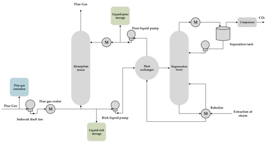
Figure 1.
Schematic diagram of the integrated flexible operation of carbon capture power plants (Includes split-flow, liquid storage operation).
The split-flow operation of carbon capture plants includes both flue gas splitting (as shown in the blue module in Figure 1) and liquid-rich splitting. By controlling the flue gas bypass, the flue gas split operation method adjusts the proportion of flue gas directly discharged to the atmosphere, thus achieving flexible adjustment of carbon capture energy consumption and net output power. The key equipment of the liquid storage operation method (as shown in the green module in Figure 1) is the solution storage, so that the rich liquid absorbed from the absorption tower and the rich liquid entering the regeneration tower at this time are no longer equal, i.e., the CO2 absorption process, which determines the amount of carbon capture, and the solution regeneration process, which determines the energy consumption of carbon capture, are decoupled to a certain extent.
The combined consideration of shunt operation and storage operation allows for both shifting the impact of carbon capture energy consumption to load during peak-load times and proactive CO2 emission when the system needs it. This integrated and flexible low-carbon operation can expand the net output range of carbon capture power plants, as shown in Figure 2.
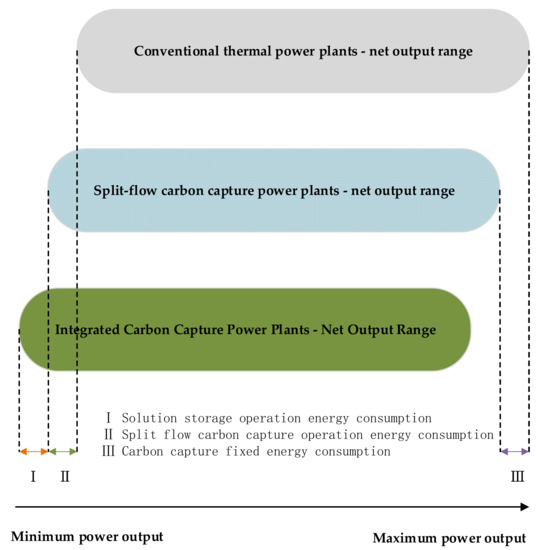
Figure 2.
Comparison of net output power of conventional thermal and carbon capture power plant (includes conventional thermal power plants, split-flow, and integrated carbon capture plants).
At peak-load times, split-flow carbon capture plants need to increase their output and accordingly produce more CO2. If all of this CO2 is captured, the carbon capture energy consumption will also be increased largely, which is not conducive to increasing the output of the carbon capture plant. If the carbon capture plant is operated in a flexible way, the CO2 at peak load can be stored in solution storage. This will help to reduce the CO2 emissions directly into the atmosphere to ensure a low carbon system. It also helps to reduce the energy consumption of carbon capture at peak load, ensuring the system’s economy.
In the low-load period, the split-flow carbon capture power plant reduces the unit output and expands the net output range mainly through the energy consumption generated during CO2 capture (Figure 2 in mode II). At the same time, the energy consumption generated by carbon capture increases the wind power consumption capacity. However, if we also consider the liquid storage type carbon capture operation, which releases CO2 from the solution storage, we can further increase the carbon capture energy consumption. The system will have a lower output limit and a larger output range (Figure 2 in mode III). At the same time, it further promotes wind power consumption. The whole process can be seen as replacing expensive high-carbon units at peak-load times by increasing wind power output at low-load times and utilizing economical low-carbon units.
In summary, the storage and liquid carbon capture method shift CO2 from the peak load to the low-load for processing. In turn, the energy consumption of the carbon capture process is delayed in the time dimension, and the expensive high-carbon thermal power plants are replaced by low-carbon carbon capture power plants and wind power plants, making the system more low-carbon and economical.
3. Low Carbon Economy Dispatch Modeling
The low carbon economic dispatch model considers wind power forecasting and integrated carbon capture power plants separately on the source side. In this paper, we use EEMD-LSTM-SVR for accurate forecasting of Belgian wind power and for low carbon dispatch we consider integrated split-flow and storage carbon capture power plants. The model is built as follows [23].
3.1. Dataset
The dataset consists of the forecast dataset and the scheduling input data. The forecast dataset consists of 15 min wind power data and six characteristic quantities for December 2021 in Belgium. The wind power is the target value, and the six characteristic quantities are EWMA, SMA, average, minimum, maximum, and average difference. Dispatch input data includes load value and 1 h wind power (averaged for 15 min wind power). When performing the dispatch, the wind power is used to match different cases, including Belgian grid forecast wind power, the actual wind power on 31 December, and the EEMD-LSTM-SVR forecast wind power.
3.1.1. EWMA and SMA Feature Construction of Wind Power
Exponential weighted moving average (EWMA) is often used to describe trends of time series. It considers the high weight of recent data and at the same time gradually reduces the weight of recent data to compensate the overall trend. This method can forecast the future trend of line loss and enrich datasets further.
The process of constructing the EWMA feature is as follows. For wind power, n is the number of observations to be monitored including . The EWMA characteristics of 15 min wind power are calculated according to Equation (1).
where is the smoothing parameter. The value range of is and differential evolution method is used to minimize the objective function to obtain the optimal value. The calculated objective is shown in Equation (2):
Simple moving average (SMA) is an unweighted arithmetic average of the n values preceding a given variable. For example, a 96-point simple moving average of a 15-min wind power forecast refers to the average of the previous day’s wind power. If the power at each point is to , and when calculating successive values, a new point is added while an old point is dropped out, the SMA is calculated as.
Figure 3 shows the Belgian wind power and its EWMA and SMA characteristics. The red line in Figure 3 is the EWMA, which reflects the trend of wind power in the short term and provides reference information for wind power forecasting. The blue line in Figure 3 is SMA. SMA is the average value of wind power at the previous N points, which is a simple extraction of wind power variation trend. EWMA can extract wind power variation trend, while eliminating the influence of complex noise and enriching the dataset.
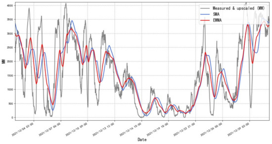
Figure 3.
EWMA and SMA characteristics of wind power data (Time Scale: December 2021).
3.1.2. Curve Feature Construction of Wind Power
Curve features include average, minimum, maximum, and average difference values, respectively, used to describe average trend and extreme value of time series data and changes of time series data on different days. For time series data of impact quantity , means impact quantity within time-window w, point changes from 1 to 4. Equations (4) and (5) show calculation of and . The time-window is set as 4 for insight into hourly changes in wind power.
Figure 4 shows the curve characteristics of wind power. Constructing curve features for wind power can maximize the use of data trends and help the model learn. Using average, extreme, and average difference values, wind power prediction models will be more sensitive. Data that is only one-dimensional is extended to four dimensions. As the amount of data increases, the model can also get better prediction results.
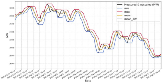
Figure 4.
Curve characteristics of wind power data (only one day’s data is shown).
3.2. EEMD-LSTM-SVR
3.2.1. EEMD
Empirical mode decomposition (EMD) is a decomposition method used to deal with non-linear and uneven signals. The wind power sequence happens to be a non-stationary original signal. The decomposition results of EMD are shown in Equation (6) [24].
where, is Intrinsic Mode Functions (IMF) and is residual.
EMD processing flow is as follows:
- (1)
- The extreme points of the original signal are demarcated, all the extreme points are collected to form the upper and lower envelope (), and is obtained by means processing for envelope ().
Calculate the residual of the original signal and :
Iterate until reaches the constraint requirements, denoted as (IMF1).
- (2)
- Calculate the difference between the original signal and IMF1 as a calculation input of new round:
- (3)
- Repeat the above steps and finally get n IMF components and residual components .
In the process of power operation, there will be intermittent signals in the wind sequences. The modal aliasing phenomenon occurs in the decomposition process of EMD, resulting in poor expression of IMF components. However, EEMD adds white noise in the original statistical line loss, which can deal with the previous problem perfectly.
The EEMD processing flow is as follows:
- (1)
- Add a group of white noise signals to the original data.
- (2)
- Perform EMD decomposition on the new sequence.
- (3)
- Repeat the EMD decomposition, adding white noise of different amplitude each time to obtain N groups of IMF components and residual sequences.
- (4)
- Perform average processing on the N groups of IMF components and integrate them to obtain the EEMD decomposition result.
Figure 5 shows the raw data of wind power in Belgium for December 2021, with data recorded every 15 min. From the figure, it can be seen that wind power is strongly volatile, but at the same time there are some regularities. Using EEMD to decompose the wind power stochasticity and to explore its regularity can help to further improve the accuracy of wind power forecasting. Figure 6 shows the EEMD decomposition of the wind power data for the Belgian grid at 15 min one note. The decomposition contains 9 IMFs, as well as the residual component.

Figure 5.
Belgium December wind power data (15 min a record; Time Scale: December 2021; the most recent forecast is wind power forecast made by the Belgian grid, measured and upscaled is the actual wind power measured).
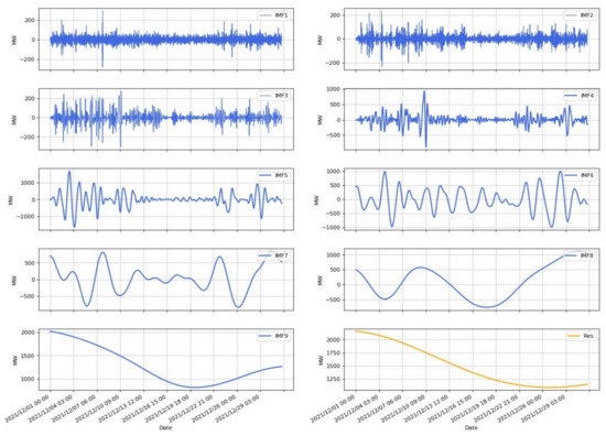
Figure 6.
Decomposition of Belgian wind power data for December using EEMD (Contains 9 IMFs and residual).
3.2.2. LSTM
LSTM solves the problem of gradient disappearance of RNN during remote transmission. LSTM currently has excellent performance in natural language processing and time series prediction. The basic unit structure diagram is shown in Figure 7 [25,26,27,28,29].
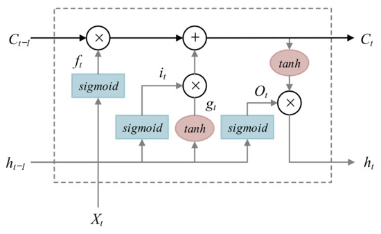
Figure 7.
Schematic diagram of the basic unit structure of LSTM [30].
In Figure 7, Xt and ht are the input and output of the basic unit at time t, it and ft are the output of the input gate and forget gate at time t respectively, Ot is the output of the output gate at time t, and gt is the unit state at time t. The specific calculation formula is as follows:
Input status.
Gating status.
Memory status.
Output status.
In the formula: is the hyperbolic tangent function, defining formula is (16); Sigmoid is sigmoid function, is an activation function, defining formula is (17); W is the weight vector; b is the bias.
It can be seen from Equations (11)–(13) that LSTM fully considers the correlation between varies data while making predictions and gives sufficient space for important information. Therefore, when performing time series data prediction, it can usually obtain more desirable results.
3.2.3. SVR
LSSVM combines the kernel function with ridge regression and uses the least squares error function to fit the data, but the amount of calculation is the third power of samples, which is not conducive to simplifying the model and improving calculating speed. On this basis, a SVR is proposed, which greatly reduces the computational complexity through support vectors and has the same ability as LSSVM to fit samples with high latitude.
The SVR regression method is widely used in time series forecasting. It has strong generalization ability in dealing with lightweight, non-linear, and time series samples. SVR non-linearly maps the input sample data to the high-dimensional feature space for linear regression, so as to perform non-linear fitting in the data space. Different from the conventional regression method, SVR introduces an insensitive loss factor . When the absolute difference between the predicted value and the actual value is less than , the calculation is stopped and the predicted result is retained. The optimization process of the SVR-based time series forecasting model is as follows [31,32,33,34,35].
Given a sample set , x is the input vector, , and is the output vector (label), . The non-linear mapping in the SVR method is defined as:
In the formula, is the input data; is the non-linear mapping function; is the weight; b is the bias. Combining principles of minimizing structural risk, the solution is transformed into an optimization problem, namely:
where L is the loss function. C is the penalty factor, used to adjust the relationship between model complexity and fitting accuracy. The larger C, the more attention will be paid to outliers. By introducing a slack variable and to correct outliers, the above problem is transformed into:
In the formula: is the insensitive loss factor, which represents the maximum allowable error, > 0. At this point, the regression problem is transformed into an objective function optimization problem. Continuing to introduce the Lagrange multiplication operator, we can get:
In the formula, and is the Lagrangian multiplier. According to Mercer’s theorem, the non-linear mapping SVR expression is:
where is the kernel function. In this paper, three kernel functions are used to compare and predict the low-frequency components of EEMD, and the kernel function with the smallest error is selected for each low-frequency component. The linear kernel, polynomial kernel, and RBF kernel are respectively Equations (24)–(26):
where, is the nuclear parameter, .
The is a very important concept in SVR, which indicates the tolerance of SVR to deviations between the predicted values of the samples and the labels. The penalty factor C acts as a constraint on . When C is a finite value, the larger the value of C, the smaller the value of should be, the narrower the isolation band, the fewer samples (with a regression loss of 0) within the band, and the greater the risk of overfitting the SVR model; while when the value of C is too small, the penalty effect of C on is too large and there is little space for to play a role. Therefore, in order to achieve good performance and at the same time reduce the risk of overfitting, the value of C must be moderate. In practice, C is the key target for tuning parameters. The insensitive loss factor , the penalty factor C, and the nuclear parameters directly determine the accuracy of the SVR method.
3.2.4. EEMD-LSTM-SVR with Cross-Validation and Grid Search Tuning
After EEMD, each IMF needs to be learned and predicted separately. Cross-validation is often applied in the process of building prediction models and validating model parameters. Specifically, existing datasets are reused and sliced using different ways, and then various combinations of training and validation sets are fed into the model, where the training set is used for model training and the validation set is excellent for validating the model. With different partitioning methods, the data that are used as training at one time may become samples in the test set in the next iteration, thus achieving cross-validation. As for time series data, incremental window cross-validation or fixed window cross-validation can be used to ensure temporal integrity as well as to prevent future data leakage. Grid search tuning is an automatic tuning method, where the optimal parameters are derived by specifying a prediction model with a given parameter tuning range. This method is more advantageous when applied to small datasets, and the sklearn library provides a function GridSearchCV specifically for debugging parameters.
Applying cross-validation to a small sample set maximizes the sample information. In addition, by repeatedly applying the trained model to new data, the overfitting can be reduced to a certain extent, thus increasing the model’s robustness. After grid tuning, the model’s training speed and prediction accuracy have been greatly improved.
After the decomposition of the wind power sequence, the processing for the different IMFs is as follows, and the flow chart is shown in Figure 8.
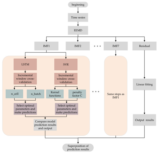
Figure 8.
Flow Chart of EEMD-LSTM-SVR with incremental cross-validation and grid search tuning.
- First, choose a suitable predicting model. This paper has two alternative predicting models: LSTM and SVR.
- Then incremental division is performed for each IMF. The data for 31 December 2021 was removed separately. This part will not participate in the training process because in predicting practical applications, this part is unknown. It is exactly the value we need to predict. The incremental division is used for the first 30 days, and the number of increments is set to 4. Figure 9 shows the schematic.
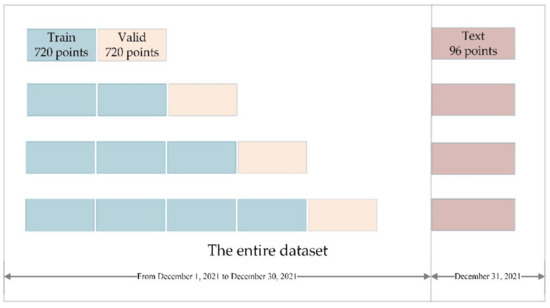 Figure 9. Incremental cross-validation schematic (15 min per point, 96 points for one day).
 - The grid search is performed for four different combinations of datasets, where the LSTM is adjusted for the number of hidden layer cells and the number of batches fed into the model each time. Specifically, the number of cells is first adjusted to deter-mine the approximate range in intervals of 10 from 10 to 100, and then the best parameters are searched for in the reduced range in units of 1. The judging criterion is the box plot of the validation loss. After determining the number of cells, it is substituted into the model and the same steps are used to search for the optimal n_batch. The other parameters of the LSTM are set as follows: the optimizer is Adam, the activation method of the fully connected layer is linear, the loss evaluation indicator is MSE, and the epochs-num in each iteration is 250.SVR mainly adjusts the kernel function and penalty factor C. The kernel function includes rbf, linear, and poly. The penalty factor C is tuned in the range from 0.01 to 100 in an isometric series with a total of 10 elements.
- After selecting a suitable prediction model for each IMF and performing cross-validation and grid tuning, the best parameters are used for prediction. The prediction results are superimposed to obtain the final statistical line loss prediction.
Among the 10 IMFs, IMF1, IMF2, IMF3, IMF4, and IMF5 are predicted by LSTM, and IMF6, IMF7, IMF8, and IMF9 are predicted by SVR. IMF10 is the residual quantity, which can be derived using linear fitting and does not require specialized prediction. For the above incremental cross-validation and grid research, each IMF varies in prediction accuracy, with IMF2 varying particularly significantly, and for visualization, IMF2 is selected for a detailed explanation.
IMF2 is a high-frequency IMF, and the first step is to predict it using LSTM. The first 2880 points of data are taken as the training set and the last day with 96 points as the test set. The test set is not involved in training throughout to avoid future data leakage during the prediction process. The training set is then divided incrementally, with the first iteration using the first 720 points of data and then using the next 720 points for validation; the second iteration adds the previous validation set to the training set, using the first 1440 points of data for training and the immediately following 720 points of data for validation and incrementally cross-validating like this. After advancing four times, all the data in the training set are well trained and learned.
The combination of cross-validation and grid search is then trained by taking cell values from 10 to 100 in units of 10, and the validation process is performed 4 times each time a new cell value is entered. Figure 10a shows the box plot of four times cross-validation for each cell value, and the overall loss level in the region from 70 to 90 is the smallest. Then the cell search is carried out again in 70 to 90 in units of 1. As shown in box Figure 10b, when the cell is 80, the box figure is the shortest and the outlier points are evenly distributed. The n_cell in the model is set to 80, and the above steps are repeated to continue the optimization search for n_batch, as shown in Figure 10c,d; firstly, the range from 10 to 100 is narrowed to 70 to 90, and then the search is conducted one by one, and the best performance is achieved when the n_batch is 87.
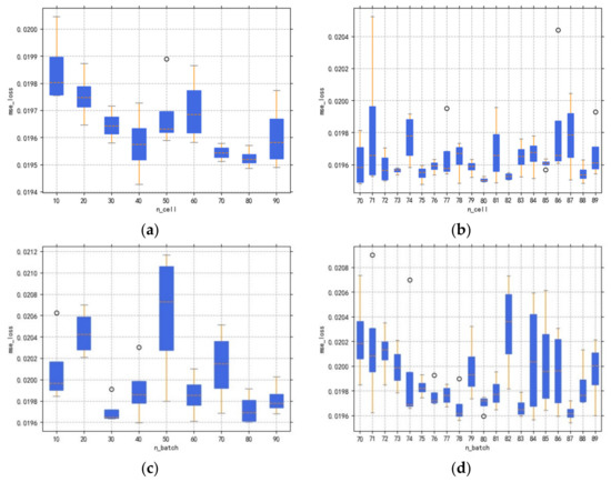
Figure 10.
IMF2 incremental cross-validation and grid search process (1. box plot; 2. n_cell: from 10 to 100 in units of 10, narrowed to 70 to 90 in units of 1, finalized 80; 3. n_batch: from 10 to 100 in units of 10, narrowed to 70 to 90 in units of 1, finalized 87; 4. the circles are outliers; (a) is cross-validation loss results for n_cell in the range 10−100; (b) is cross-validation loss results for n_cell in the range 70−90; (c) is cross-validation loss results for n_batch in the range 10-100; (d) is cross-validation loss results for n_batch in the range 70−90).
In Figure 11, measured and upscaled [MW] is the raw data of wind power recorded every 15 min on 31 December 2021 by the Belgian grid, and most recent forecast [MW] is the forecast of the Belgian grid for wind power by itself. As seen by the green line in the figure, the accuracy of the forecast is not particularly good, the RMSE is 141.027 MW, and the forecast accuracy needs to be further improved. After using the EEMD-LSTM-SVR model prediction proposed in this paper, the RMSE of the model prediction is 38.470 MW, which is reduced by 72%, as shown by the blue line in Figure 11. After applying incremental cross-validation and grid tuning reference, the model prediction accuracy is further improved again, and the RMSE is 31.802 MW, which is reduced by 17.33% based on the EEMD-LSTM-SVR. Table 1 is MSE, RMSE, MAE, MAPE, SMAPE%, and R2 of 3 cases. Table 2 is description of hyperparameters.
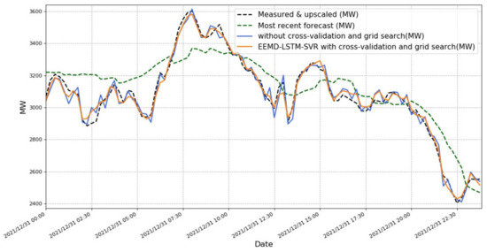
Figure 11.
Comparison of whether to use incremental cross-validation and grid tuning for the EEMD-LSTM-SVR model (measured and upscaled is the measured wind power; most recent forecast is the wind power forecast that comes with the Belgian grid).

Table 1.
Results evaluation (contains three forecast results and five evaluation indicators).
Table 2.
Description of hyperparameters (adjusted hyperparameters and their ranges in incremental cross-validation and grid search).
According to the different characteristics of IMFS, the high-frequency components IMF1–5 are predicted by LSTM. SVR predicts the low-frequency components IMF6–9 due to their regularity in order to speed up the model training. As shown in Figure 11, we can see that the tip of the orange curve is more moderate and closer to the real line loss. This demonstrates that the use of incremental cross-validation and grid search can effectively prevent model overfitting and improve model prediction accuracy. The use of grid search ensures the accuracy of the model predictions, and the predictions perform better at both the time shift and the tip of the curve. Furthermore, using cross-validation and plotting box plots ensures that the predicted values are not the result of chance for a single iteration. By increasing the training set in bulk, the impact of the dataset on the prediction results is effectively reduced and the robustness of the model is ensured [36].
3.3. Low Carbon Dispatch Modeling Considering Wind Power Forecasting and Integrated Carbon Capture Power Plants
In the low-carbon dispatch model, load is provided by low-carbon emitting carbon capture power plants, zero-carbon emitting wind farm, and high-carbon emitting conventional thermal power plants. Furthermore, wind power is made closer to the real value by accurate forecasting model. In addition, by sharing the backup pressure of thermal power plants through integrated carbon capture plants, it helps to reduce the number of thermal power starts, optimizing the low-carbon effect while reducing start-up and shutdown costs [37,38,39].
3.3.1. Optimization Objective
In this paper, we construct a low-carbon dispatch model with the system integrated cost optimization as the objective function.
where is the total cost of power system dispatch and operation; is the total cost of thermal unit start-up and shutdown; is the cost of carbon trading; is the cost of thermal fuel; is the cost of wind abandonment penalty; is the depreciation cost of carbon capture equipment.
- (1)
- Total start-up and shutdown costs of thermal power units and fuel costs .where, is the unit cost of thermal unit i on and off; n is the total number of thermal units; is the thermal unit on and off status: 1 is on, 0 is off; is the total output of thermal unit i at time t; , , are the fuel cost parameters of thermal unit i.
- (2)
- Carbon trading costs .where is the carbon trading price; is the net carbon emission of a dispatch cycle of the power system; is the length of the time period; is the carbon quota factor of thermal power units.
- (3)
- Cost of wind abandonment penalty . To improve the wind power absorption, the model includes the abandoned wind penalty cost, which is calculated as.where is the abandoned wind penalty cost factor; is the predicted wind power output at time t; is the wind power used at time t.
- (4)
- Depreciation cost of carbon capture equipment .where is the total price of carbon capture equipment except for the storage tank under the base condition; is the cost required for the expansion and renovation of the regeneration tower compressor; ω is the net salvage rate; is the depreciable life of carbon capture equipment except for the storage tank; is the price of the storage tank per unit volume; is the volume of the storage tank; is the depreciable life of the storage tank.
3.3.2. Constraints
- (1)
- Power balance constraint.
- (2)
- Integrated carbon capture power plant constraints.
The total output of carbon capture power plant includes net output power and carbon capture energy consumption. Among them, carbon capture energy consumption includes fixed energy consumption and operation energy consumption. The mathematical model of the integrated carbon capture power plant studied in this paper is shown in Equation (34).
where is the carbon capture equivalent power of thermal unit i at time t; is the carbon capture maintenance energy consumption of thermal unit i; is the maximum total output power of thermal unit i; is the CO2 treatment rate of thermal unit i at time t; is the total CO2 emission rate of thermal unit i at time t, is the flue gas split ratio of thermal unit i at time t; is the CO2 supply rate of the storage tank of thermal unit i at time t; is the net CO2 emission rate of thermal unit i at time t.
The CO2 extracted from the solution memory exists in the form of compounds in the alcohol-amine solution, and the relationship between the mass of CO2 and the volume of the alcohol-amine solution needs to be considered. In this paper, the mass of CO2 that can be extracted from the solution memory is converted into the form of the solution volume as shown in Equation (35).
where is the volume of solution required to release CO2 at time t from the solution memory installed in plant i; and are the molar masses of MEA and CO2, respectively; is the regeneration tower resolution; is the concentration of the alcoholamine solution; is the density of the alcoholamine solution.
The reservoir volume of the solution storage will have a large impact on the operation of the carbon capture plant. The reservoir volume is constrained as shown in Equation (36).
where is the amount of liquid-rich tank storage in thermal unit i at time t; is the amount of liquid-poor tank storage in thermal unit i at time t; is the configuration tank capacity of thermal unit i; is the initial liquid-rich tank storage in thermal unit i; is the initial liquid-poor tank storage in thermal unit i; is the liquid-poor tank storage in thermal unit i at the end of dispatch cycle; is the liquid-poor tank storage in thermal unit i at the end of dispatch cycle.
In addition, since the carbon capture plant was converted from a coal-fired power plant, the total output limits, climbing constraints, and start-up and shutdown constraints are the same as those for conventional coal-fired power plants.
- (3)
- Rotation standby constraint
In order to deal with the uncertainty of wind power and load, this paper uses thermal power units and carbon capture units to jointly provide the required rotating backup of the system, as shown in Equation (37).
where is the maximum net output power of the i-th thermal unit; is the minimum net output power of the i-th thermal unit; is the net output up-ramping rate of the i-th thermal unit at time t; is the net output down-ramping rate of the i-th thermal unit at time t; is the standby capacity factor considering load uncertainty, % is the standby capacity factor considering wind power uncertainty; is the installed capacity of wind farm.
The standby constraint for thermal power units is shown in Equation (38).
where is the minimum output power of thermal unit i; is the maximum output power of thermal unit i; is the downward climbing rate of thermal unit i; is the upward climbing rate of thermal unit i.
The carbon capture unit standby constraint is shown in Equation (39).
where: is the upper limit of output of carbon capture unit i; is the lower limit of output of carbon capture unit i.
4. Case Study and Operational Cases
Firstly, EEMD-LSTM-SVR is used for the forecast of wind power in Belgium in December, and the hourly forecast of wind power is shown in Figure 12, where the black line is the raw wind power in Belgium, the blue line is the forecast made by the Belgian grid, and the red line is the result of wind power forecast in this paper. Wind power forecasts for each IMF are shown in Figure 13. The installed capacity of wind power in Belgium is 4883.397 MW. In order to match the system size, the wind power data is shrunk by a factor of 10.
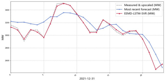
Figure 12.
Graph of raw wind power data and hourly forecast results for Belgium (measured and upscaled is the measured wind power; most recent forecast is the wind power forecast that comes with the Belgian grid; EEMD-LSTM-SVR is wind power forecast results in this paper).
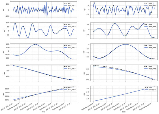
Figure 13.
Graph of the forecast results of each IMF for wind power (15 min; Contains 9 IMFs and residual).
The algorithm in this chapter uses the improved IEEE-39 nodal system, which includes ten thermal power units and three wind farms in the system. Among them, wind farms of 198.5 MW, 191.5 MW, and 98.3 MW are introduced in nodes 9, 19, and 22, respectively. If the system introduces carbon capture power plants, G1 and G2 are converted into carbon capture power plants, and if the system does not introduce, they are conventional thermal power units. Load and wind power data refer to Belgian data. The specific thermal unit parameter data are detailed in Table 3, and other parameters of the system are shown in Table 4. This chapter is solved optimally by CPLEX.
Table 3.
Thermal power unit parameters (total of 10 thermal units; input parameters include operation, cost, creep parameters, and carbon capture intensity).
Table 4.
Other system parameters (mainly system size parameters and carbon capture plant operating and cost parameters).
To verify the effectiveness of the low carbon dispatch model proposed in this paper, five operational scenarios are set up in this paper for comparison:
- Case 1: using wind power forecast data from the Belgian grid without carbon capture power plants.
- Case 2: using wind power forecast data from the Belgian grid, including split-flow carbon capture plants.
- Case 3: using Belgian grid wind forecast data with integrated flexible operation mode carbon capture plants.
- Case 4: using actual wind power data from the Belgian grid as of December 31, including integrated flexible operation carbon capture plants.
- Case 5: wind power forecasts using EEMD-LSTM-SVR, including integrated flexible-operating carbon capture plants.
5. Result
5.1. Analysis of Dispatch Results
In this paper, we consider the low-carbon economic dispatch of the system under the above five cases, to verify the operational advantages of the dispatch model proposed in this paper, and the dispatch results are shown in Table 5.
Table 5.
Dispatch results (dispatch costs, carbon emissions, and wind abandonment for five cases).
As shown in Table 5, compared with Case 1, the carbon emission and wind abandonment of Case 2 are reduced by 7262.173 t and 333.995 (MWh) respectively, thus verifying the positive effect of carbon capture power plant on low carbon economic dispatch. Case 3 adopts solution memory for carbon capture energy time shift, and its cost is increased by 5.9% compared with Case 2, but the carbon emissions are reduced and there is no wind abandonment. Case 3, 4, and 5 all use integrated carbon capture plants. Case 5 uses EEMD-LSTM-SVR for wind power prediction, and the cost is closest to the real value because the wind power is closer to the real value, with a difference of only USD 60. Case 4 uses the wind power predicted by the Belgian grid, and the total cost of dispatch differs from the actual value by USD 2149. Thus, the advantages of the optimization model proposed in this paper are verified. With accurate wind power prediction, the dispatching results will be more realistic and help dispatchers to make decisions.
5.2. Unit Dispatch Situation Analysis
Figure 14 shows the dispatching of units from Case 1. It can be seen that if the carbon capture plant is not added, there will be wind abandonment during the period 0:00–9:00. The reason for this is that the system takes into account the start-up and shutdown situation, so a certain amount of wind power must be discarded to achieve the economic optimum, and closely related to the start-up and shutdown of thermal power units is the peak-to-valley difference in net output of thermal power.
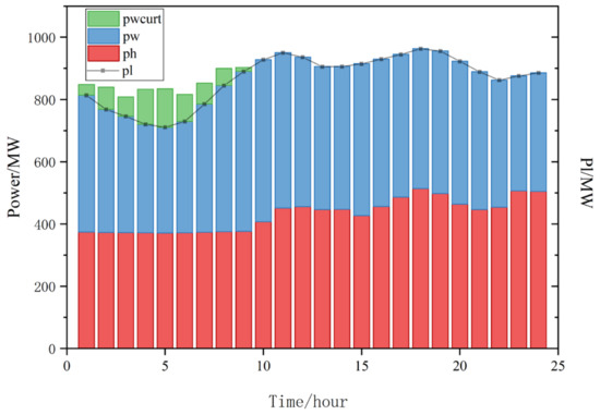
Figure 14.
Case 1 unit dispatching (pwcurt is wind abandonment; pw is wind power output; ph is thermal power unit output; pl is system load).
Figure 15 shows the thermal power output for five cases. It can be seen that Case 4 and Case 5 have the smallest peak-to-valley differences, which proves the validity of the reservoir energy time-shift characteristics and the use of wind power forecasting to bring the dispatch results closest to the real situation. Case 3 does show a downward adjustment of the peak-to-valley difference compared to Case 2. The main reason for the difference between peak and trough is the difference in energy consumption of carbon capture.
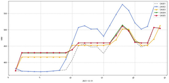
Figure 15.
Five scenes thermal power output.
Figure 16 shows the carbon capture energy consumption. From the figure, it can be seen that the maximum carbon capture energy consumption of Cases 3,4,5 is higher than that of Case 2, because Cases 3,4,5 can reach the maximum carbon capture treatment energy consumption through the CO2 provided by the storage tank. Meanwhile, the carbon capture energy consumption of Case 2 is less in the load valley and more in the peak, because to ensure the low-carbon operation of the system, the shunt carbon capture plant will try to absorb the emitted CO2, and the amount of absorbed CO2 is coupled with the amount of carbon capture, resulting in the situation that the larger the net output of the thermal power plant, the larger its carbon capture energy consumption. Cases 3,4,5, on the other hand, have more carbon capture energy consumption in the load valley and less carbon capture energy consumption in the load peak, which reduces the peak-to-valley difference of the total thermal power output, due to the energy time-shifting characteristics of the storage tank.
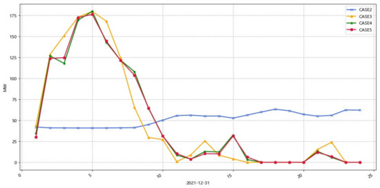
Figure 16.
Cases 2–5: carbon capture energy consumption.
Figure 17 shows the change of the total storage volume of G1 and G2 thermal power plants in Case 3. As can be seen from the figure, the trend of the total storage volume of G1 and G2 is to release CO2 in the load valley (the storage volume of the rich tank decreases and the storage volume of the poor tank increases), which makes the carbon capture equipment processing energy consumption higher, and to store CO2 in the load peak (the storage volume of the rich tank increases and the storage volume of the poor tank decreases), which makes the carbon capture equipment processing energy consumption lower and realizes energy time shift, which lays the foundation for low carbon economic dispatch, compared with the shunt type This can further reduce carbon emissions compared to split-flow carbon capture power plants.
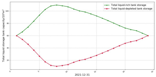
Figure 17.
Change of the total storage volume of G1 and G2 thermal power plants in Case 3 (liquid-rich; depleted tanks).
As can be seen from Figure 18, Case 1 has higher carbon emission because there is no carbon capture power plant; while the carbon emission difference between Cases 2, 3, 4, and 5 is mainly at the peak-load time, with higher carbon emission at the peak of Case 2 and lower carbon emission at Cases 3, 4, and 5, mainly because the high carbon thermal power is higher at the peak load of Case 2 and low at the high carbon thermal power of Cases 3, 4, and 5.
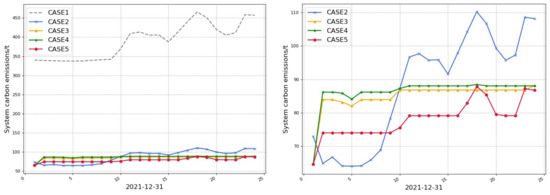
Figure 18.
Carbon emissions of five cases (the right figure is a partial enlargement of Cases 2–5 for perspective).
6. Conclusions
This paper constructs an integrated carbon capture power plant power system dispatch model with wind power prediction, investigates the accuracy of wind power prediction, and analyzes the dispatching economics due to the energy time-shift characteristics of carbon capture power plants. Detailed conclusions are as follows:
- Compared with conventional thermal power plants, carbon emissions will be reduced by 77.548% with split type carbon capture power plants and by 78.248% with integrated type carbon capture power plants. This proves that carbon capture power plants can effectively reduce carbon emissions.
- In the economic dispatch of the power system, compared with the split carbon capture power plant, the integrated carbon capture power plant can reduce carbon emissions by 10.847%, which proves the effectiveness of the integrated carbon capture power plant in reducing carbon emissions.
- In terms of wind power prediction accuracy improvement, compared with the wind power predicted by the Belgian grid, the total cost of dispatching using the wind power predicted in this paper will be closer to the real situation, with a difference of only 60$.
- Compared with the traditional thermal power plants, the inclusion of the split carbon capture plant reduces the amount of abandoned wind by 53.525%; with the integrated carbon capture plant, the plot energy of wind power can be fully utilized. It proves the effectiveness of integrated carbon capture power plant for absorbing wind power.
- In future work, the economic dispatch of power systems containing carbon capture power plants at multiple time scales will be considered. Meanwhile, the research in this paper does not involve demand-side standby and flexible dispatch, and subsequent studies such as standby-assisted market decision will be considered.
Author Contributions
Conceptualization, C.D., Y.Z., Q.D. and K.L.; methodology, C.D., Y.Z.; software, Y.Z.; validation, Q.D., K.L. and C.D.; formal analysis, Y.Z.; investigation, Y.Z.; resources, C.D.; writing—original draft preparation, Y.Z.; writing—review and editing, Y.Z., C.D., Q.D. and K.L.; visualization, Y.Z.; supervision, C.D.; project administration, C.D. All authors have read and agreed to the published version of the manuscript.
Funding
This research received no external funding.
Institutional Review Board Statement
Not applicable.
Informed Consent Statement
Not applicable.
Data Availability Statement
Data available in a publicly accessible repository that does not issue DOIs. Publicly available datasets were analyzed in this study. This data can be found here: (Wind-powergeneration (elia.be)).
Conflicts of Interest
The authors declare no conflict of interest.
Abbreviations
The following abbreviations are used in this manuscript:
| ARIMA | AR Integrated Moving Average |
| CCS | Carbon Capture and Storage |
| CEEMDAN | Complete Ensemble Empirical Mode Decomposition with Adaptive Noise |
| CNN | Convolutional Neural Networks |
| EMD | Empirical Mode Decomposition |
| EEMD | Ensemble Empirical Mode Decomposition |
| ENN | Error Encoding Network |
| EWMA | Exponential Weighted Moving Average |
| ICEEMDAN | Improved Complete Ensemble Empirical Mode Decomposition with Adaptive Noise |
| IMF | Intrinsic Mode Functions |
| LSSVM | Least Squares Support Vector Machines |
| LSTM | Long Short-Term Memory recurrent neural network |
| MEMD | Median EMD |
| MLP | Multilayer Perceptron |
References
- Chen, H.-H.; Hof, A.F.; Daioglou, V.; de Boer, H.S.; Edelenbosch, O.Y.; van den Berg, M.; van der Wijst, K.-I.; van Vuuren, D.P. Using Decomposition Analysis to Determine the Main Contributing Factors to Carbon Neutrality across Sectors. Energies 2022, 15, 132. [Google Scholar] [CrossRef]
- Bi, X.; Yang, J.; Yang, S. LCA-Based Regional Distribution and Transference of Carbon Emissions from Wind Farms in China. Energies 2022, 15, 198. [Google Scholar] [CrossRef]
- Arraño-Vargas, F.; Shen, Z.; Jiang, S.; Fletcher, J.; Konstantinou, G. Challenges and Mitigation Measures in Power Systems with High Share of Renewables—The Australian Experience. Energies 2022, 15, 429. [Google Scholar] [CrossRef]
- Mustafayev, F.; Kulawczuk, P.; Orobello, C. Renewable Energy Status in Azerbaijan: Solar and Wind Potentials for Future Development. Energies 2022, 15, 401. [Google Scholar] [CrossRef]
- Zhang, Z.; Santoni, C.; Herges, T.; Sotiropoulos, F.; Khosronejad, A. Time-Averaged Wind Turbine Wake Flow Field Prediction Using Autoencoder Convolutional Neural Networks. Energies 2022, 15, 41. [Google Scholar] [CrossRef]
- Zhu, T.; Guo, Y.; Li, Z.; Wang, C. Solar Radiation Prediction Based on Convolution Neural Network and Long Short-Term Memory. Energies 2021, 14, 8498. [Google Scholar] [CrossRef]
- Quan, H.; Srinivasan, D.; Khosravi, A. Short-Term Load and Wind Power Forecasting Using Neural Network-Based Prediction Intervals. IEEE Trans. Neur. Net. Lear. Syst. 2014, 25, 303–315. [Google Scholar] [CrossRef]
- Du, J.; Yue, C.; Shi, Y.; Yu, J.; Sun, F.; Xie, C.; Su, T. A Frequency Decomposition-Based Hybrid Forecasting Algorithm for Short-Term Reactive Power. Energies 2021, 14, 6606. [Google Scholar] [CrossRef]
- Mao, L.; Xu, J.; Chen, J.; Zhao, J.; Wu, Y.; Yao, F. A LSTM-STW and GS-LM Fusion Method for Lithium-Ion Battery RUL Prediction Based on EEMD. Energies 2020, 13, 2380. [Google Scholar] [CrossRef]
- Bokde, N.; Feijóo, A.; Al-Ansari, N.; Tao, S.; Yaseen, Z.M. The Hybridization of Ensemble Empirical Mode Decomposition with Forecasting Models: Application of Short-Term Wind Speed and Power Modeling. Energies 2020, 13, 1666. [Google Scholar] [CrossRef] [Green Version]
- Mora, E.; Cifuentes, J.; Marulanda, G. Short-Term Forecasting of Wind Energy: A Comparison of Deep Learning Frameworks. Energies 2021, 14, 7943. [Google Scholar] [CrossRef]
- Thuraisingham, R.A. Revisiting ICEEMDAN and EEG rhythms. Biomed. Signal Proces. Control 2021, 68, 102701. [Google Scholar] [CrossRef]
- Bokde, N.D.; Tranberg, B.; Andresen, G.B. Short-term CO2 emissions forecasting based on decomposition approaches and its impact on electricity market scheduling. Appl. Energy 2021, 281, 116061. [Google Scholar] [CrossRef]
- Zhang, J.; Williams, S.O.; Wang, H. Intelligent computing system based on pattern recognition and data mining algorithms, Sustain. Comput. Infor. Syst. 2018, 20, 192–202. [Google Scholar]
- Xia, Y.; Zhao, J.; Ding, Q.; Jiang, A. Incipient Chiller Fault Diagnosis Using an Optimized Least Squares Support Vector Machine with Gravitational Search Algorithm. Front. Energy Res. 2021, 9, 717. [Google Scholar] [CrossRef]
- Chen, T.; Song, M.; Hui, H.; Long, H. Battery Electrode Mass Loading Prognostics and Analysis for Lithium-Ion Battery–Based Energy Storage Systems. Front. Energy Res. 2021, 9, 543. [Google Scholar] [CrossRef]
- Bokde, N.D.; Feijóo, A.; Al-Ansari, N.; Yaseen, Z.M. A comparison between reconstruction methods for generation of synthetic time series applied to wind speed simulation. IEEE Access 2019, 7, 135386–135398. [Google Scholar] [CrossRef]
- Liu, Z.; Li, L.; Tseng, M.L.; Tan, R.R.; Aviso, K.B. Improving the Reliability of Photovoltaic and Wind Power Storage Systems Using Least Squares Support Vector Machine Optimized by Improved Chicken Swarm Algorithm. Appl. Sci. 2019, 9, 3788. [Google Scholar] [CrossRef] [Green Version]
- Zheng, Q.; Yan, P.; Zareipour, H.; Niya, C. A review and discussion of decomposition-based hybrid models for wind energy forecasting applications. Appl. Energy 2019, 235, 939–953. [Google Scholar]
- Ma, L. Inter-Provincial Power Transmission and Its Embodied Carbon Flow in China: Uneven Green Energy Transition Road to East and West. Energies 2022, 15, 176. [Google Scholar] [CrossRef]
- Olaleye, A.K.; Wang, M.; Kelsall, G. Steady state simulation and exergy analysis of supercritical coal-fired power plant with CO2 capture. Fuel 2015, 151, 57–72. [Google Scholar] [CrossRef]
- Theo, W.L.; Lim, J.S.; Hashim, H.; Mustaffa, A.A.; Ho, W.S. Review of pre-combustion capture and ionic liquid in carbon capture and storage. Appl. Energy 2016, 183, 1633–1663. [Google Scholar] [CrossRef]
- LI, J.; WEN, J.; HAN, X. Low-carbon unit commitment with intensive wind power generation and carbon capture power plant. J. Mod. Power Syst. Clean Energy 2015, 3, 63–71. [Google Scholar] [CrossRef] [Green Version]
- Sun, S.; Wei, L.; Xu, J.; Jin, Z. A New Wind Speed Forecasting Modeling Strategy Using Two-Stage Decomposition, Feature Selection and DAWNN. Energies 2019, 12, 334. [Google Scholar] [CrossRef]
- Elsaraiti, M.; Merabet, A. A Comparative Analysis of the ARIMA and LSTM Predictive Models and Their Effectiveness for Predicting Wind Speed. Energies 2021, 14, 6782. [Google Scholar] [CrossRef]
- Alharbi, F.R.; Csala, D. Wind Speed and Solar Irradiance Prediction Using a Bidirectional Long Short-Term Memory Model Based on Neural Networks. Energies 2021, 14, 6501. [Google Scholar] [CrossRef]
- Sigalo, M.B.; Pillai, A.C.; Das, S.; Abusara, M. An Energy Management System for the Control of Battery Storage in a Grid-Connected Microgrid Using Mixed Integer Linear Programming. Energies 2021, 14, 6212. [Google Scholar] [CrossRef]
- Mohammad, F.; Ahmed, M.A.; Kim, Y.-C. Efficient Energy Management Based on Convolutional Long Short-Term Memory Network for Smart Power Distribution System. Energies 2021, 14, 6161. [Google Scholar] [CrossRef]
- Xie, Y.; Ueda, Y.; Sugiyama, M. A Two-Stage Short-Term Load Forecasting Method Using Long Short-Term Memory and Multilayer Perceptron. Energies 2021, 14, 5873. [Google Scholar] [CrossRef]
- Chung, J.; Gulcehre, C.; Cho, K.H.; Bengio, Y. Empirical evaluation of gated recurrent neural networks on sequence modeling. arXiv 2014, arXiv:1412.3555. [Google Scholar]
- Khan, P.W.; Byun, Y.-C.; Lee, S.-J.; Kang, D.-H.; Kang, J.-Y.; Park, H.-S. Machine Learning-Based Approach to Predict Energy Consumption of Renewable and Nonrenewable Power Sources. Energies 2020, 13, 4870. [Google Scholar] [CrossRef]
- Kim, Y.; Hur, J. An Ensemble Forecasting Model of Wind Power Outputs Based on Improved Statistical Approaches. Energies 2020, 13, 1071. [Google Scholar] [CrossRef] [Green Version]
- Tang, M.; Chen, W.; Zhao, Q.; Wu, H.; Long, W.; Huang, B.; Liao, L.; Zhang, K. Development of an SVR Model for the Fault Diagnosis of Large-Scale Doubly-Fed Wind Turbines Using SCADA Data. Energies 2019, 12, 3396. [Google Scholar] [CrossRef] [Green Version]
- Kim, K.; Hur, J. Weighting Factor Selection of the Ensemble Model for Improving Forecast Accuracy of Photovoltaic Generating Resources. Energies 2019, 12, 3315. [Google Scholar] [CrossRef] [Green Version]
- Tan, B.; Ke, X.; Tang, D.; Yin, S. Improved Perturb and Observation Method Based on Support Vector Regression. Energies 2019, 12, 1151. [Google Scholar] [CrossRef] [Green Version]
- Abualigah, L.; Zitar, R.A.; Almotairi, K.H.; Hussein, A.M.; Abd Elaziz, M.; Nikoo, M.R.; Gandomi, A.H. Wind, Solar, and Photovoltaic Renewable Energy Systems with and without Energy Storage Optimization: A Survey of Advanced Machine Learning and Deep Learning Techniques. Energies 2022, 15, 578. [Google Scholar] [CrossRef]
- Jin, J.; Wen, Q.; Zhang, X.; Cheng, S.; Guo, X. Economic Emission Dispatch for Wind Power Integrated System with Carbon Trading Mechanism. Energies 2021, 14, 1870. [Google Scholar] [CrossRef]
- Liu, J.; Sun, W.; Harrison, G.P. Optimal Low-Carbon Economic Environmental Dispatch of Hybrid Electricity-Natural Gas Energy Systems Considering P2G. Energies 2019, 12, 1355. [Google Scholar] [CrossRef] [Green Version]
- Wang, X.; Zhou, Y.; Tian, J.; Wang, J.; Cui, Y. Wind Power Consumption Research Based on Green Economic Indicators. Energies 2018, 11, 2829. [Google Scholar] [CrossRef] [Green Version]
Publisher’s Note: MDPI stays neutral with regard to jurisdictional claims in published maps and institutional affiliations. |
© 2022 by the authors. Licensee MDPI, Basel, Switzerland. This article is an open access article distributed under the terms and conditions of the Creative Commons Attribution (CC BY) license (https://creativecommons.org/licenses/by/4.0/).