Pressure Drop and Energy Recovery with a New Centrifugal Micro-Turbine: Fundamentals and Application in a Real WDN

Abstract

Water distribution networks need to improve system efficiency. Hydropower is a clean and renewable energy that has been among the key solutions to environmental issues for many decades. As the turbine is the core of hydropower plants, high attention is paid to creating new design solutions and increasing the performance of turbines in order to enhance energy efficiency of leakage by pressure control. Hence, design and performance analysis of a new turbine is a crucial aspect for addressing the efficiency of its application. In this study, computational fluid dynamics (CFD) modeling is coupled with experimental tests in order to investigate the optimal performance of a new centrifugal turbine. The behavior of the flow through the turbine runner is assessed by means of velocity profiles and pressure contours at all components of the machine under different operating conditions. Finally, the turbine geometry is scaled to a real water distribution network and an optimization procedure is performed with the aim of investigating the optimal location of both the designed new centrifugal micro-turbines (CMT) and pressure reducing valves (PRV) in order to control the excess of pressure and produce energy at the same time.

1. Introduction

Hydropower is a well-advanced technology that convert the potential energy of water into electric energy [1,2,3] and contributes to about 50% of the all existing renewable energy sources [4,5]. It is reported that at least 16% of worldwide energy production results from the hydraulic power generation [6,7].

The turbine represents the core device of any hydropower plant, converting the hydraulic energy in mechanical energy of a rotating shaft [8], which is then converted into an electrical current by means of a generator. Turbines can operate under steady-state or transient operations in hydropower plants [9]: the angular frequency of the runner, as well as the discharge through the turbine, is constant in the former case and varies over time for transient operations [10]. Moreover, steady-states include both best efficiency point (BEP) conditions and off-design conditions, such as part load (PL), high load (HL), and full load (FL), whereas transient operations include start-stops and load variations [11,12]. The operation of a turbine is significantly complex and is characterized by high turbulence, even in steady-state conditions [13]. When the runner is supplied by a constant angular frequency, between the trailing edge of the guide vane and leading edge of the runner blade an exchange of momentum occurs, known as a rotor-stator interaction [14,15], causing the propagation of a sound wave in all directions [16]. In addition, away from the BEP, the turbine is affected by a large variation in velocity and pressure, which can result in output power swings, as well as in mechanical vibrations that can damage the machine in the long term [17]. In transient conditions, the development of fatigue to the runner and wear and tear of the turbine components have also been observed [18] due to fluctuant pressure loadings and mechanical stresses varying in magnitude, direction and frequency [19]. A thorough analysis is therefore required to investigate the phenomena affecting the flow behavior within a turbine in order to improve the efficiency and power output with increased operational stability [20]. An improvement in performance of the turbine and its components definitely results in the improvement of overall hydropower plant efficiency [21]. Computational fluid dynamics (CFD) is a well-known reliable technique for performing a careful design [22,23] and simulation of hydraulic turbines [24,25]. A computational approach allows one to investigate minor details of flow, which cannot be caught by simple experiments [8,26]. A huge selection of studies based on CFD approaches to investigate design and behavior of turbomachines is available in the literature. Among the studies on turbines, Aghaei Tog et al. (2008) [27] showed an advanced turbulence model in CFD analysis of radial turbines and presented an accurate way to select turbulent parameters for FLUENT [28] users, applying this software as a complementary design tool for high-speed turbo-machinery components. Chen et al. (2008) [29] defined an advanced aerodynamic system to optimize blade design by the use of parametric modeling and optimization strategy modules. Biesinger et al. (2010) [30] used numerical techniques (i.e., phase-shift and time-inclining methods) to investigate unsteady flow phenomena for a more efficient future-generation turbine blade design. Wang et al. (2012) [31] investigated a novel design of a composite material axial water turbine, relying on a three-dimensional numerical flow analysis. The flow characteristics were investigated at different components of the turbine, and both the exact torque and power were analyzed at different rotating speeds. With reference to pumps as turbines (PATs), several studies investigated steady turbulent flows by CFD analysis [32,33,34], and other works have studied unsteady flow fields by means of a moving mesh technique in CFD codes [35,36].

The aim of this work is to investigate the optimal performance of a new centrifugal turbine by using both computational fluid dynamics modeling and experimental tests on a laboratory prototype. The experimental measurements in terms of flow rate, pressure-drop, torque and rotational speed allow one to assess the turbine behavior under different operating conditions. Such experimental tests have been crucial in performing a CFD analysis, providing the boundary conditions needed to properly model the reference turbine. Based on the CFD simulation in the whole flow passage, the analysis of three-dimensional steady flows is carried out under both design and off-design conditions. Pressure contours and pressure drops across the runner are provided to assess the entity of losses within the turbine components for different rotational speeds. Moreover, velocity profiles at the inlet and outlet of the runner are compared in order to analyze the behavior of the vanes in guiding the fluid exiting from the volute, as well as to quantify any slip phenomena at the outlet of the runner, which may occur owing to the limited number of blades. Moreover, the application of the turbine to a real case study network is presented. An optimization procedure is carried out to investigate the optimal scale design of the machine, as well as the optimal number and position of such designed turbines together with pressure reducing valves, in order to maximize both water and energy savings and minimize the investment costs. In this study, the optimization has been applied to a new mathematical model, including, in a comprehensive way, the optimization constraints, as well as turbine design formulations and the equations modeling the hydraulic behavior of the network.

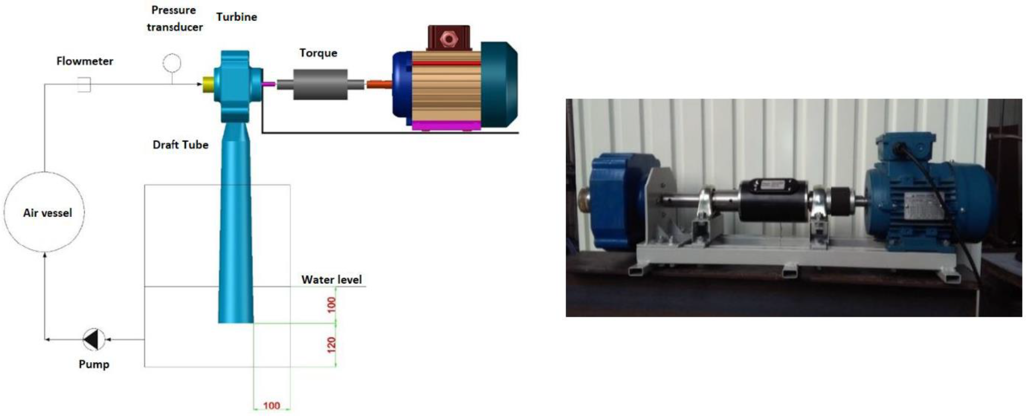
2. Experimental Tests

Modeling the geometry of a centrifugal turbine involves defining the impeller and volute components. In this study the geometric modeling of the draft tube has also been considered, as it is one of the crucial components of a turbine. Performance tests have been carried out with reference to a centrifugal turbine prototype (Figure 1) in order to assess the hydraulic behavior profile under different operating conditions.

The experimental setup consists of a free surface reservoir, on the top of which a turbine is installed with a low-return suction tube. The setup is also equipped with an air vessel to control sudden pressure impulses, a flow-control circulation pump, and all required hydraulic and electrical components, such as a permanent magnet generator (or SEIG) and energy dissipation for flow control.

The turbine prototype is characterized by an intake external diameter of 46 mm (40 mm inside) and a shaft diameter of 12 mm (Figure 2). The turbine is installed on a rigid base and connected to a generator. A datum torque meter (model M425-S2-B) is installed between the turbine shaft and the electric brake.

In the first stage of the tests, the turbine is experimented with variable pressure, flow and variable speed, keeping the opening guide vane at maximum to establish the performance points. The measured values are flow, pressure, torque and rotational speed. During the tests, the flow was varied within the range of 19–46 L/s, whereas the head drop was kept as 32.8 m (3.17 bar). The measured torque range was 25–50 N·m., whereas the rotational speed varied between 750 and 1850 rpm. Finally, the power on the turbine shaft was between 2 and 10 kW. The experimental points are shown in

Table 1. Experimental results of the turbine prototype.

D (mm)			150
H (m)			32.8
Q (L/s)	19.49	27.98	34.1	39.19	43.72	46.26
Q (%)	42	60	74	85	95	100
η (%)	33	40	52	55	62	65
N (rpm)	767	1064	1489	1580	1792	1843
P (W)	2040	3590	5680	6930	8710	9690
V (m/s)	0.97	1.39	1.70	1.95	2.17	2.30
T (N m)	25.40	32.22	36.43	41.88	46.41	50.21
Ph (W)	6265	8994	10,961	12,597	14,053	14,870

D—impeller diameter; H—head drop; Q—flow discharge; η—efficiency; N—rotational speed; P—mechanical power; V—flow velocity; T—torque; P_h—hydraulic power.

.

3. Numerical Model

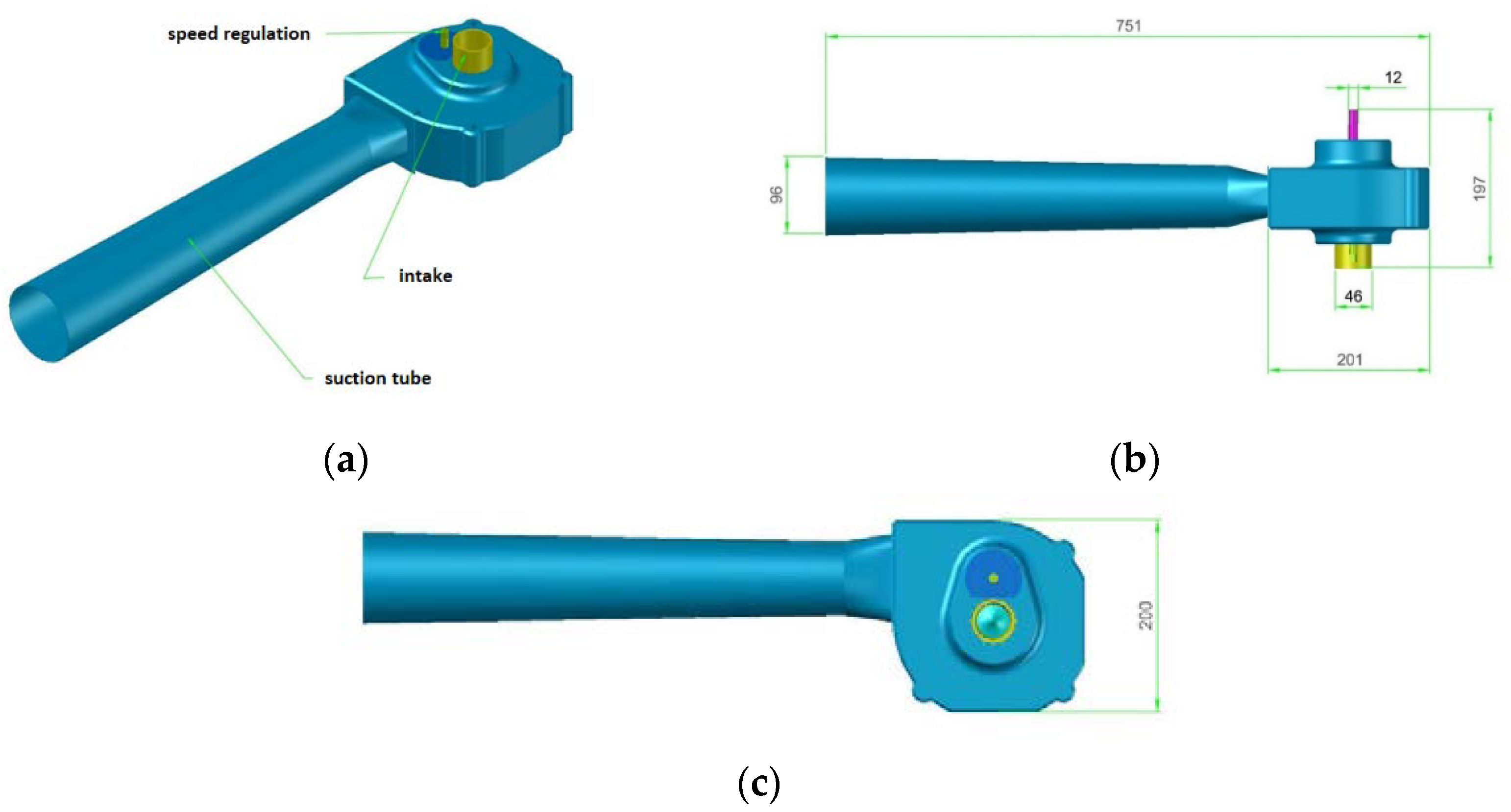
3.1. Turbine Geometry and Boundary Conditions

Providing a qualitative and quantitative prediction of fluid, CFD tools represent an important technological advance toward a detailed analysis of the flow behavior. CFD modeling allows one to study the behavior of both turbulent and laminar flows, as well as exchanges of energy, flow phases, vorticity and turbulence levels. Based on the experimental data provided as boundary conditions, as well as the virtual prototype of the turbine (Figure 1), a turbine modeling was performed with the aid of a CFD software for turbulent 3D flow and a design/drafting software. In particular, the software COMSOL Multiphysics [37] was selected for the CFD modeling in terms of geometry modification, mesh generation, calculation and results analysis, presenting accurate results for several fluid flow problems. COMSOL is a finite element method (FEM) software, relying on the mass conservation and the RANS (Reynolds-averaged Navier-Stokes) equations. FEM is a computational method according to which an object is divided into smaller elements. Each element is assigned to a set of characteristic equations, which are then solved as a set of simultaneous equations to investigate the behavior of the whole object [38].The design of each machine component was, instead, performed by the software AutoCAD [39] and then imported by COMSOL to reproduce the physical problem and post-processing capabilities. The CFD approach was mainly intended to investigate the complex internal flows through all components of the machine at different operating conditions, which may be crucial to improve the performance of the machine at off-design conditions. The simulations were performed by using the k-ε model for turbulent flows (with Reynolds number ranging between 20,850 and 209,000), assuming water as an incompressible fluid and the fluid regime as steady state. This model exhibits a good convergence rate and relatively low memory requirements. A crucial assumption on which the k-ε model is based is that the Reynolds number is high enough. Moreover, such a model assumes that the turbulence is in equilibrium in boundary layers, which means that the production equals the dissipation. Being not always verified, such assumptions limit the accuracy of the model. Furthermore, in case of rotating flows, such a model often shows poor agreement with experimental data [40]. However, the flow close to the surface of the blade is turbulent; thus, the assumptions used to derive the k-ε model are not valid there. The correction of the k-ε model to better describe the flow in regions near the blades is not always desirable due to the significantly high resolution requirements. Analytical expressions, well known as wall functions, are instead preferred to describe the flow in the critical regions [41] and are used in this application. Wall functions ignore the flow field in the buffer region and analytically compute a nonzero fluid velocity [40,41,42]. When wall functions are used, the wall lift-off in viscous units ${\mathsf{\delta }}_{\mathrm{w}}^{+}$ has to be thoroughly verified to be below 30 in the whole region. In case of ${\mathsf{\delta }}_{\mathrm{w}}^{+}$ greater than the threshold value, a finer boundary layer mesh is added.

All calculations were performed on an Intel 5, CPU 3.90 GHz, RAM 8 GB with four cores and threads running in parallel. The model uses a physics-controlled mesh, according to which the size attributes and operation sequences are automatically defined; thus, the mesh is automatically generated and adapted for the model’s physics settings. Hence, once the geometric model was defined, the automatic mesh generation was performed by a careful selection of the related parameters, in order to achieve good precision results with an acceptable computational effort. The mesh near the surface of the blade was refined by an additional fine mesh to solve turbulence equations. Based on the assessment of the accuracy of the calculated maximum pressure, a mesh convergence analysis was tested by the use of a finer mesh and, thus, a greater number of degrees of freedom (DOF). In particular, local sizing and curvature size functions were used to obtain a sufficiently fine mesh to properly capture regions characterized by a rapid change in key variables, such as pressure and flow velocity. According to the mesh convergence analysis, for a mesh of approximately 150,000 DOF, the computed pressure value increased from 0.1 to 2.0 bar for a mesh of approximately 1,000,000 DOF, showing that 500,000 DOF provides the same precision as 1,000,000 DOF. Finally, the fluid domain was constructed with 280,056 tetrahedral components, with 85% of quality element. This number of elements is a compromise between the mesh quality as computed by the automatic mesh generator and the computational capacity. Nevertheless, as demonstrated in [43], the number of elements and their size ensure for limited error in the calculation of global parameters. The good agreement between calculation and experimental results in terms of global parameters, as shown below in Section 3.2, demonstrates the accuracy of the numerical solution.

The analyzed domain consists of an inlet, an outlet and two periodic interfaces. The boundary conditions at the inlet and outlet parts of the turbine were set according to the experimental measurements. In particular, the pressure value recorded by the pressure transducer located downstream of the draft tube was assumed as boundary condition at the outlet, whereas the flow discharge was considered as the the boundary condition at the inlet.

Hence, for each simulation, the rotation of the impeller was assumed as the rotational speeds achieved experimentally, and such a rotating domain was considered as a moving mesh. This definition regulates the spatial frame and applies to all interfaces of physics where domains rotate. Thus, in a rotating coordinate system in the inner domain, and in the outer one in fixed coordinates, these interfaces formulate the Navier-Stokes equations for incompressible fluids which are expressed in Equation (1) [44]:

$$\begin{gathered} \nabla ·\mathrm{V}=0 \\ \mathsf{\rho }\frac{\partial \mathrm{V}}{\partial \mathrm{t}}+\mathsf{\rho }\mathrm{V}·\nabla \left(\mathrm{V}\right)=-\nabla \mathrm{p}+\nabla ·\left(\mathsf{\mu }\left(\nabla \mathrm{V}+\nabla {\mathrm{V}}^{\mathrm{T}}\right)\right)+\mathrm{F} \end{gathered}$$

(1)

where μ is the dynamic viscosity, $\mathsf{\rho }$ the fluid density, $\mathrm{p}$ the pressure and $\mathrm{F}$ is the external forces applied to the fluid. Non-rotating parts can be considered as fixed parts, which were coupled with the rotating parts by means of an identity pair set, that is, the fluid continuity boundary condition.

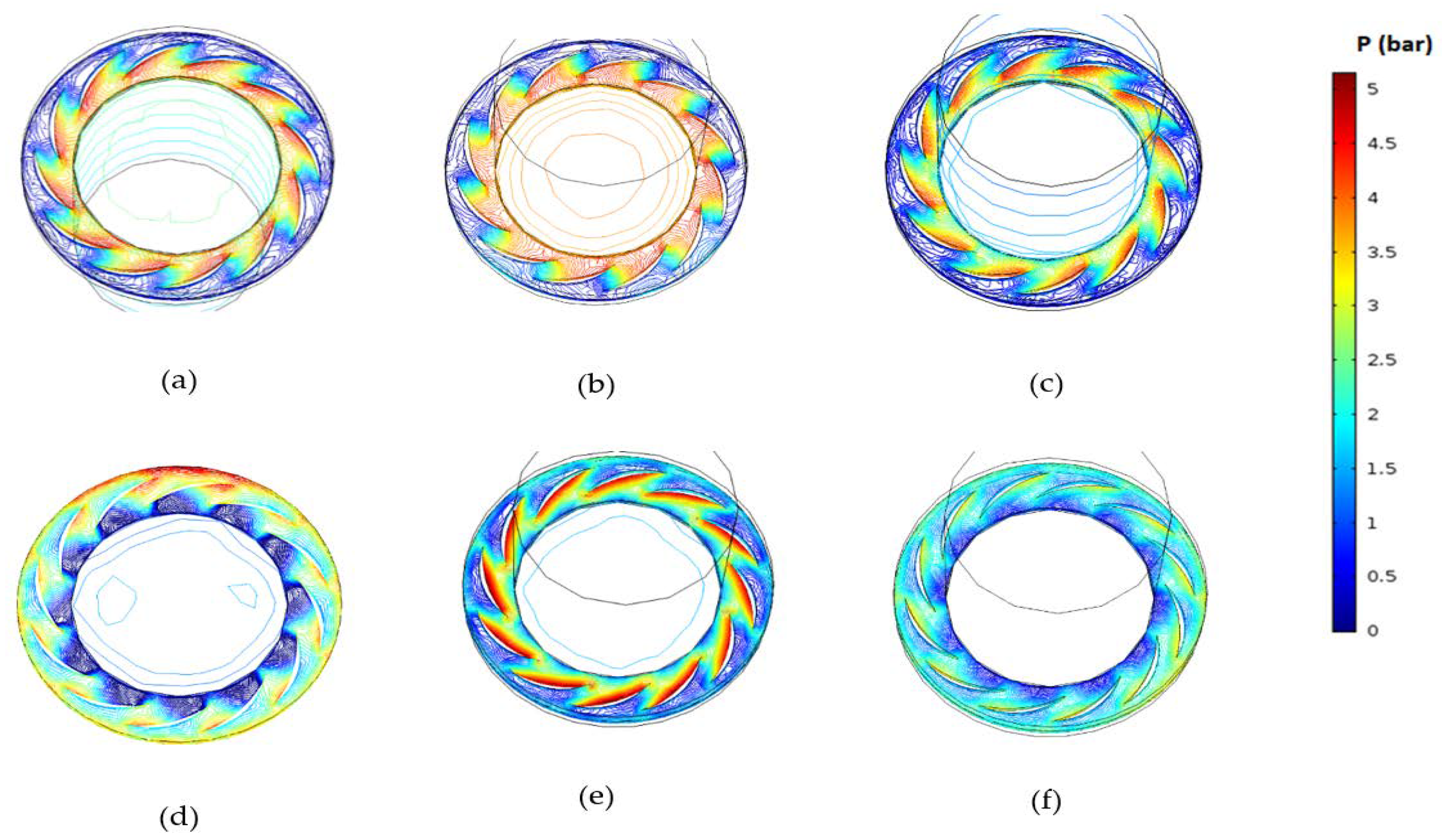
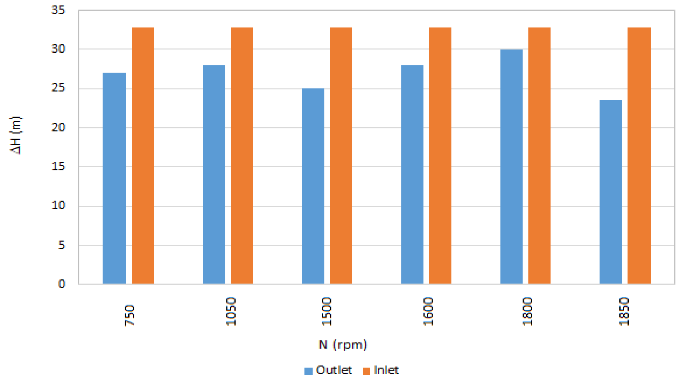
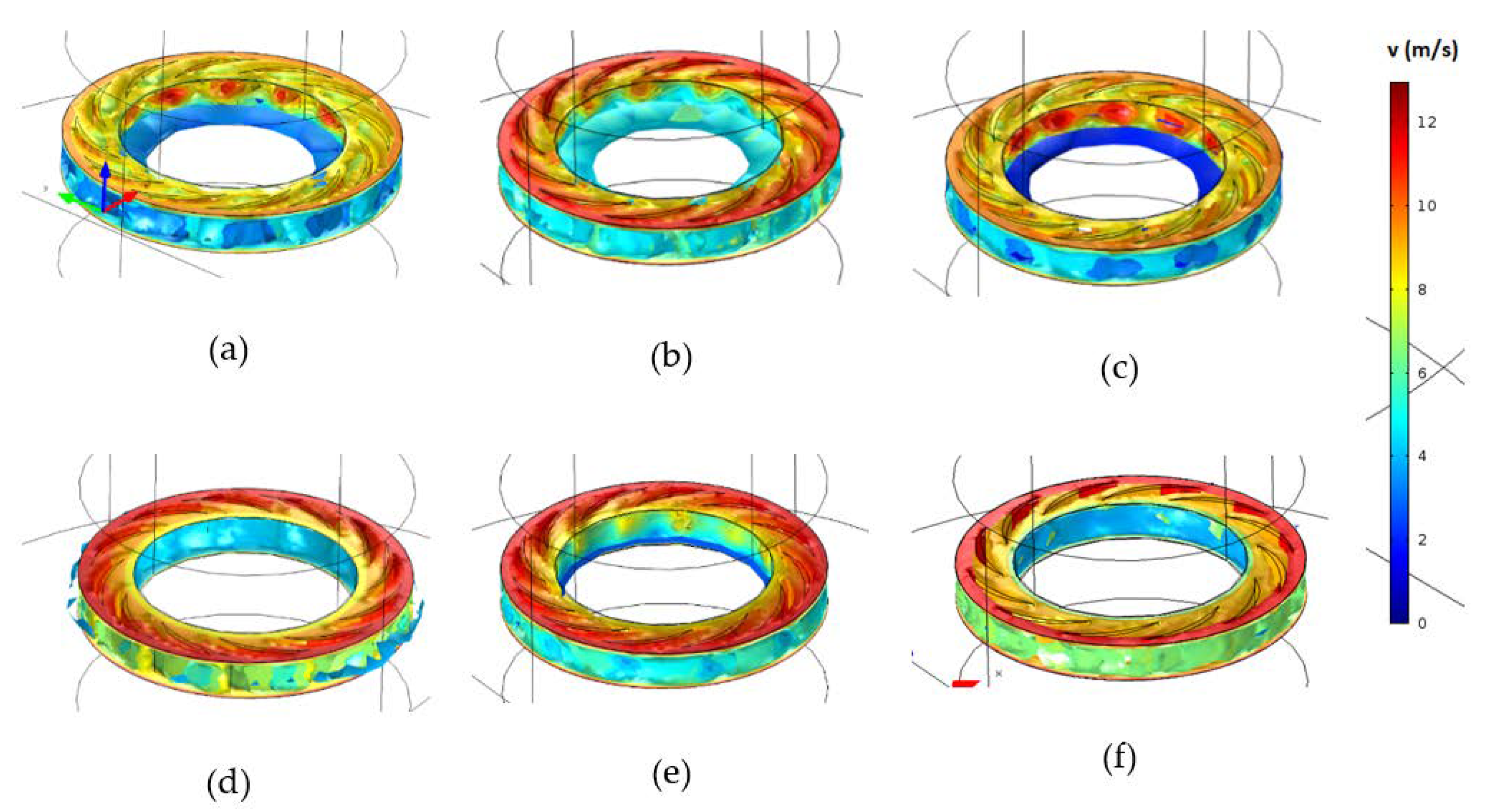
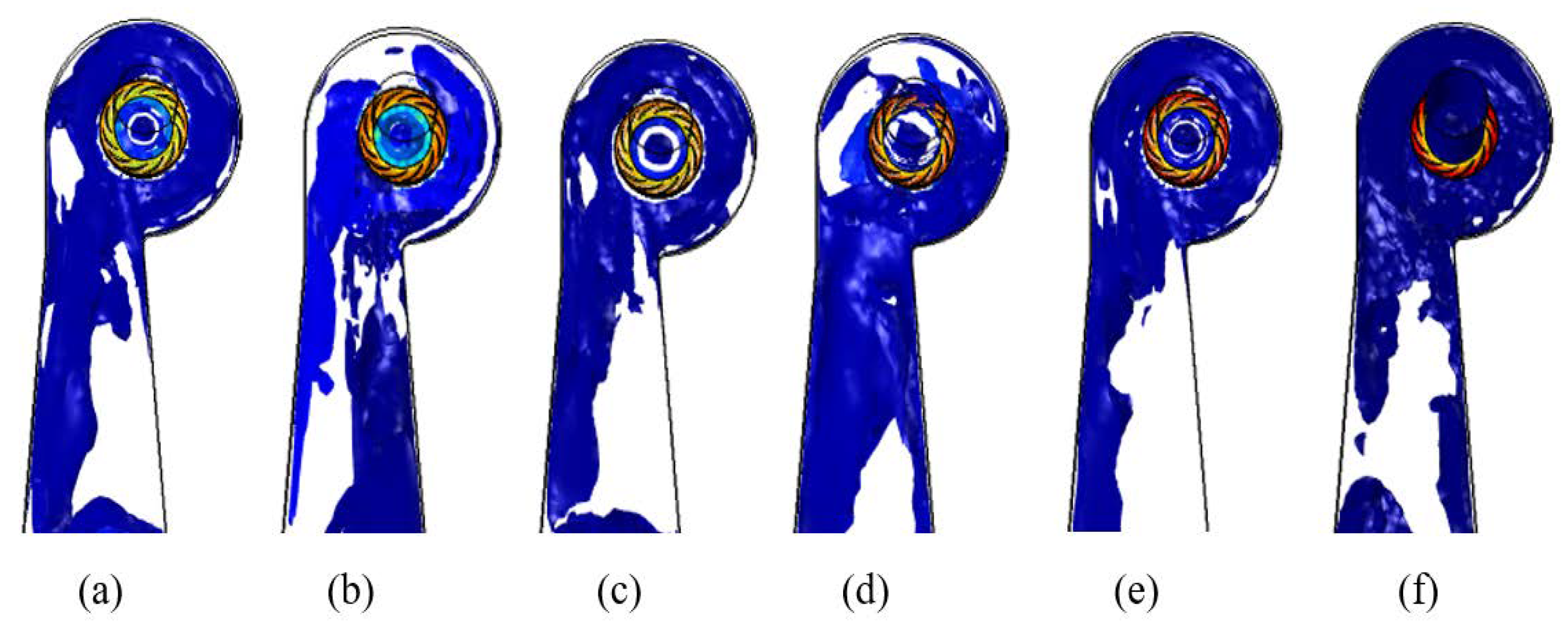
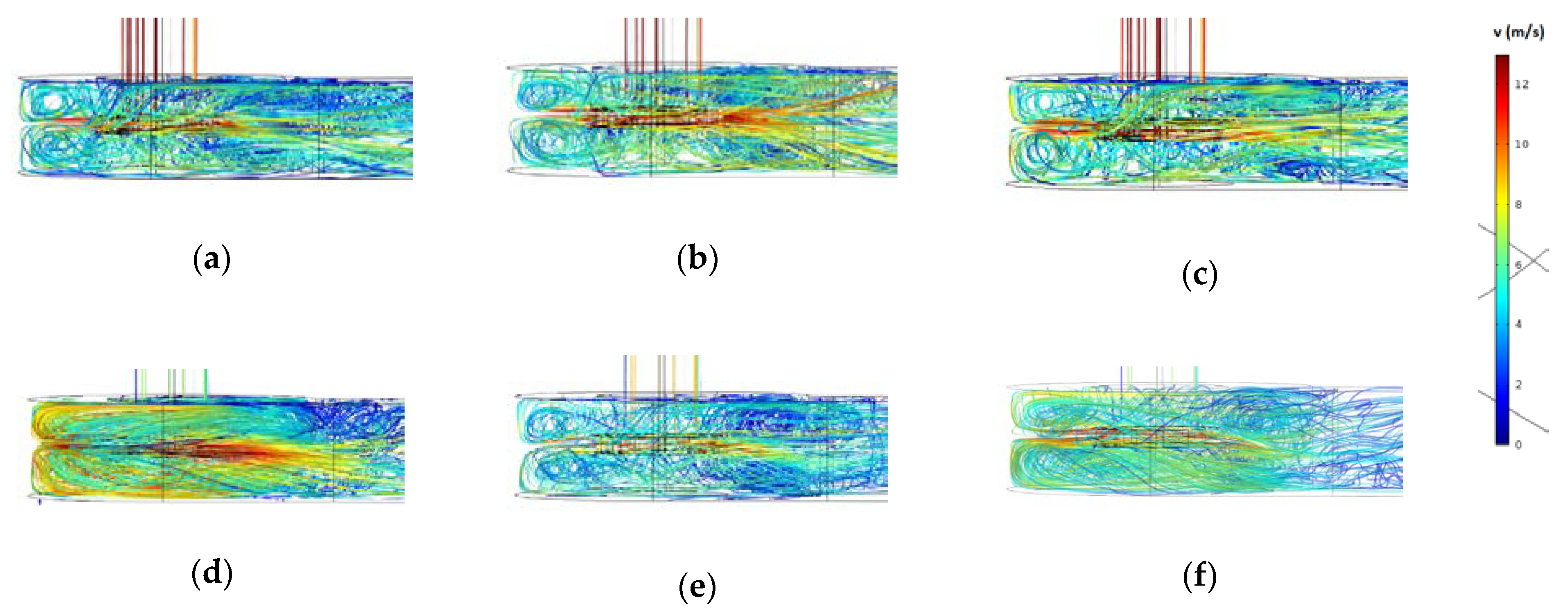
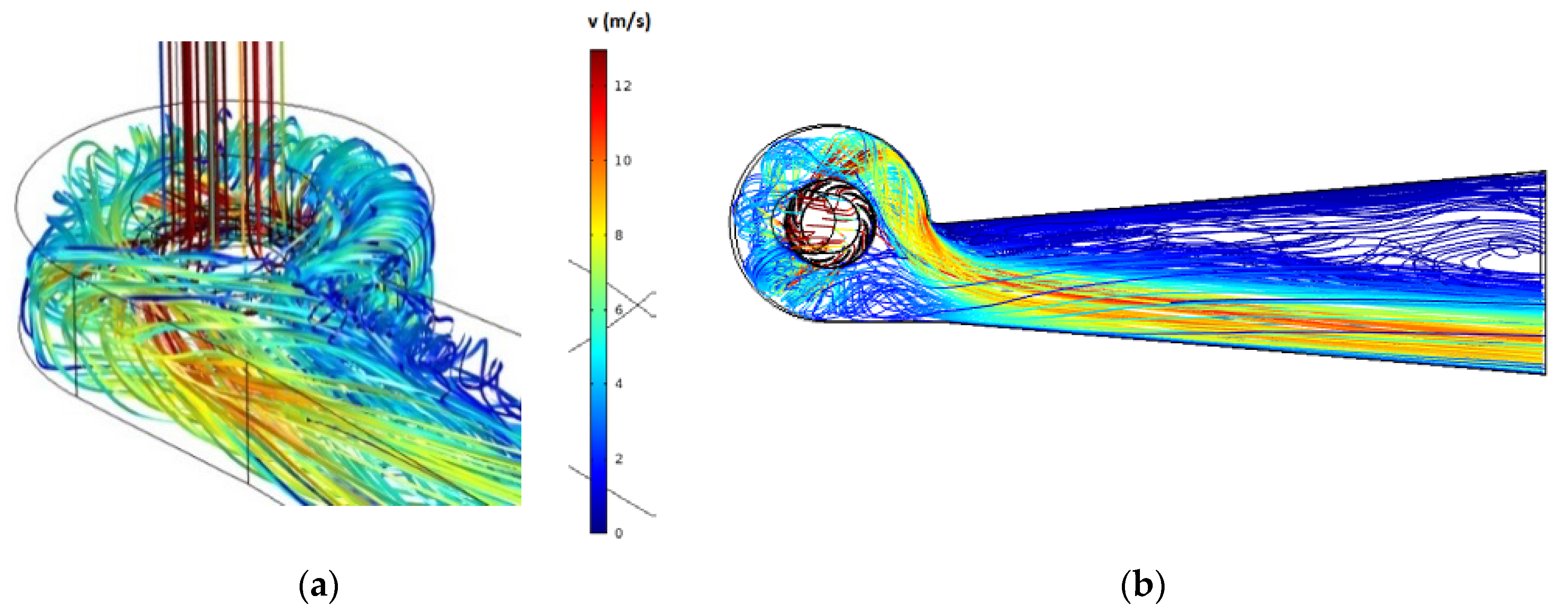
3.2. Numerical Results

The design of a turbine impeller is generally based on given values of differential head, flow rate and rotating speed. This means that the specific speed is practically imposed. Hence, the novel geometry was designed to target the specific speed resulting from the experimental results. Thus, the turbine was simulated for different rotational speeds (varying between 700 and 1800 rpm), different flow values (ranging between 19 and 50 L/s), and keeping the head drop value at 32.8 m.

Figure 3 shows the total pressure contours across the runner of the turbine for different rotational speeds.

Figure 4 shows the total pressure drop at the inlet and outlet rotor for different rotational speeds. According to this figure, such a difference in terms of pressure drop is quite small for most rotational speeds. Instead, a more significant difference is detected for a rotational speed equal to 1850 rpm.

A comparison of the flow velocity for different rotational speeds is presented in Figure 5. It is clearly shown that the geometry is more resistive to the flowrate for N < 1500 rpm for a given range of the total pressure drop. This results in a higher change in absolute kinetic energy over the range of pressure differentials, causing a higher change in dynamic pressure.

Figure 6 represents for each rotational speed the velocity isosurface at the first instant the turbine is crossed by flow and starts to rotate. According to Figure 6, the turbine response becomes faster by increasing the rotational speed. The fastest response is attained at a rotational speed at 1850 rpm.

Figure 7 shows the velocity field at six operating points in a section plan of the turbine runner. The characteristics of the flow were analyzed in critical regions, such as near the hub and tip zones. With reference to Figure 7a, high flow acceleration is present from the leading to the trailing edge, but at 68% along the blade chord, a sudden increase in static pressure is observed, causing flow deceleration. Figure 7b,c shows almost the same conditions as in Figure 7a, with a sharper velocity magnitude near the trailing edges. Figure 7c–f shows some differences in terms of flow velocities, with higher values in the regions near the hub. The degree of flow deceleration is lower when compared with N < 1500 rpm, inducing lower internal losses as well.

Figure 8 presents the velocity streamlines between the runner and the guide vane. According to the streamline trend, it is clear that the fluid moves radially outward in the rotor boundary layer. With reference to Figure 9, the velocity contour shows that the maximum velocity reaches about 12 m/s in the region close to the leading edge of the rotating blade, whereas the minimum velocity occurs close to the right side of the vane.

Dimensional analysis is a useful and powerful tool to analyze complex problems and solve different technical/physical problems. Thus, non-dimensional hydraulic feature terms of the machine were described in accordance with the geometric and kinetic resemblance principles:

$$\mathsf{\psi }=\frac{\mathrm{gH}}{{\mathrm{N}}^2{\mathrm{D}}^2}$$

(2)

$$\mathsf{\phi }=\frac{\mathrm{Q}}{{\mathrm{ND}}^3}$$

(3)

$$\mathsf{\tau }=\frac{\mathrm{T}}{{\mathsf{\rho }\mathrm{N}}^2{\mathrm{D}}^5}$$

(4)

Non-dimensional quantities defined by Equations (2)–(4) represent the head coefficient, the flow coefficient and the torque coefficient of the centrifugal turbine, respectively.

Figure 10 shows the comparison between experimental measurements and numerical results. Scale effects, due to design parameters not perfectly adherent to real parameters, lead to a deviation between the prototype and the numerical model. In addition, since the Reynolds number of the model is typically higher than the prototype, losses of friction resulting from the CFD analysis are larger than the prototype. In addition, the model efficiency is generally greater because of the viscous effects associated with vortex or eddy effects. The maximum efficiency of the tested is attained as 65% for a value of the flow coefficient as about 0.45.

According to Figure 10, the comparison between CFD and experimental tests predicted that CFD results are slightly higher than the experimental results.

Based on experimental results and affinity laws, the following relationships were obtained:

$$\mathsf{\phi }={ \mathrm{q}}_{\mathrm{T}} \mathsf{\alpha }\sqrt{\mathsf{\psi }}$$

(5)

$$\mathrm{N}=\frac{{\mathrm{n}}_{\mathrm{T}}}{\mathrm{D}} \sqrt{\mathrm{gH}}$$

(6)

$$\mathsf{\eta }=1-\left(0.4\right){\left(\frac{75}{1000 \mathrm{D}}\right)}^{0.25}{\left(\frac{5}{\mathrm{H}}\right)}^{0.1}$$

(7)

where ${\mathrm{q}}_{\mathrm{T}}$ and ${\mathrm{n}}_{\mathrm{T}}$ are experimental coefficients equal to 0.141 and 22.76, respectively, whereas $\mathsf{\alpha }$ is the runner thickness.

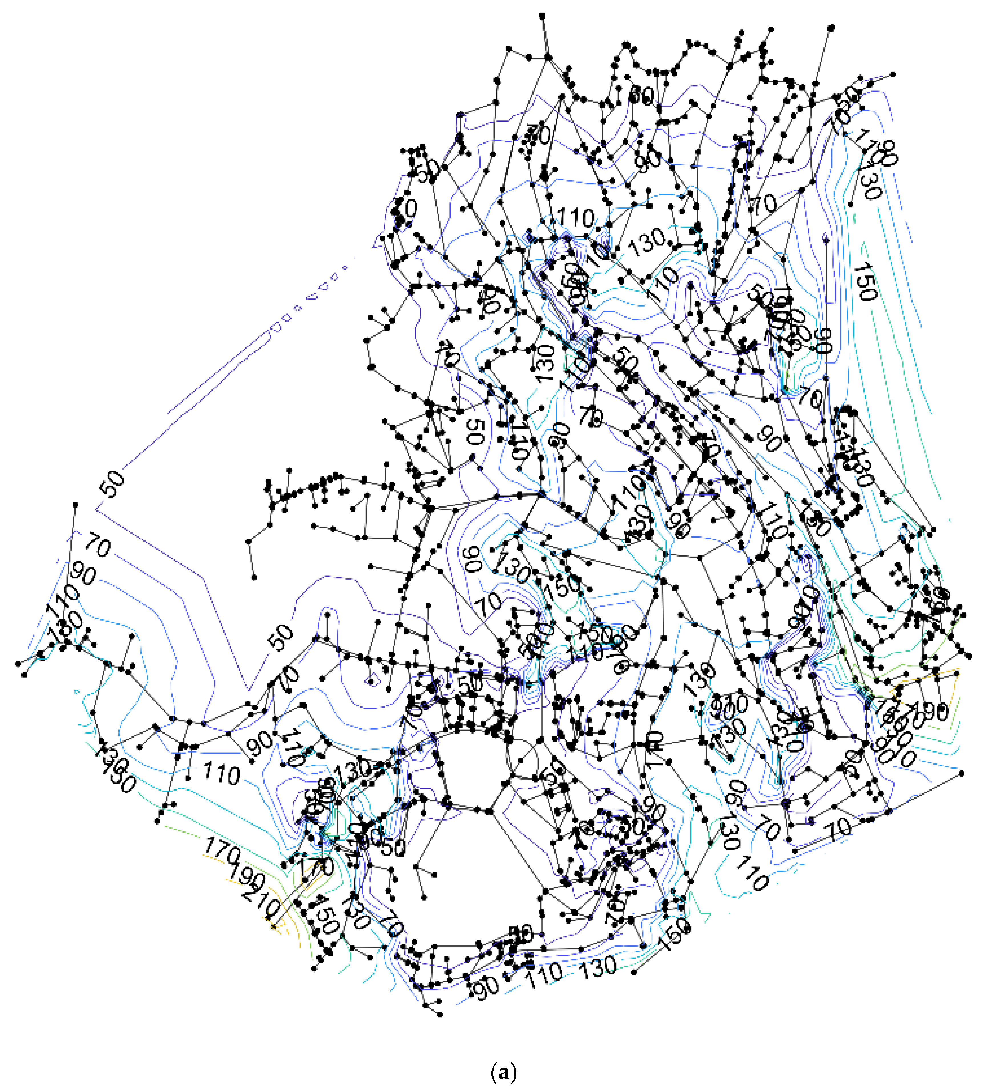
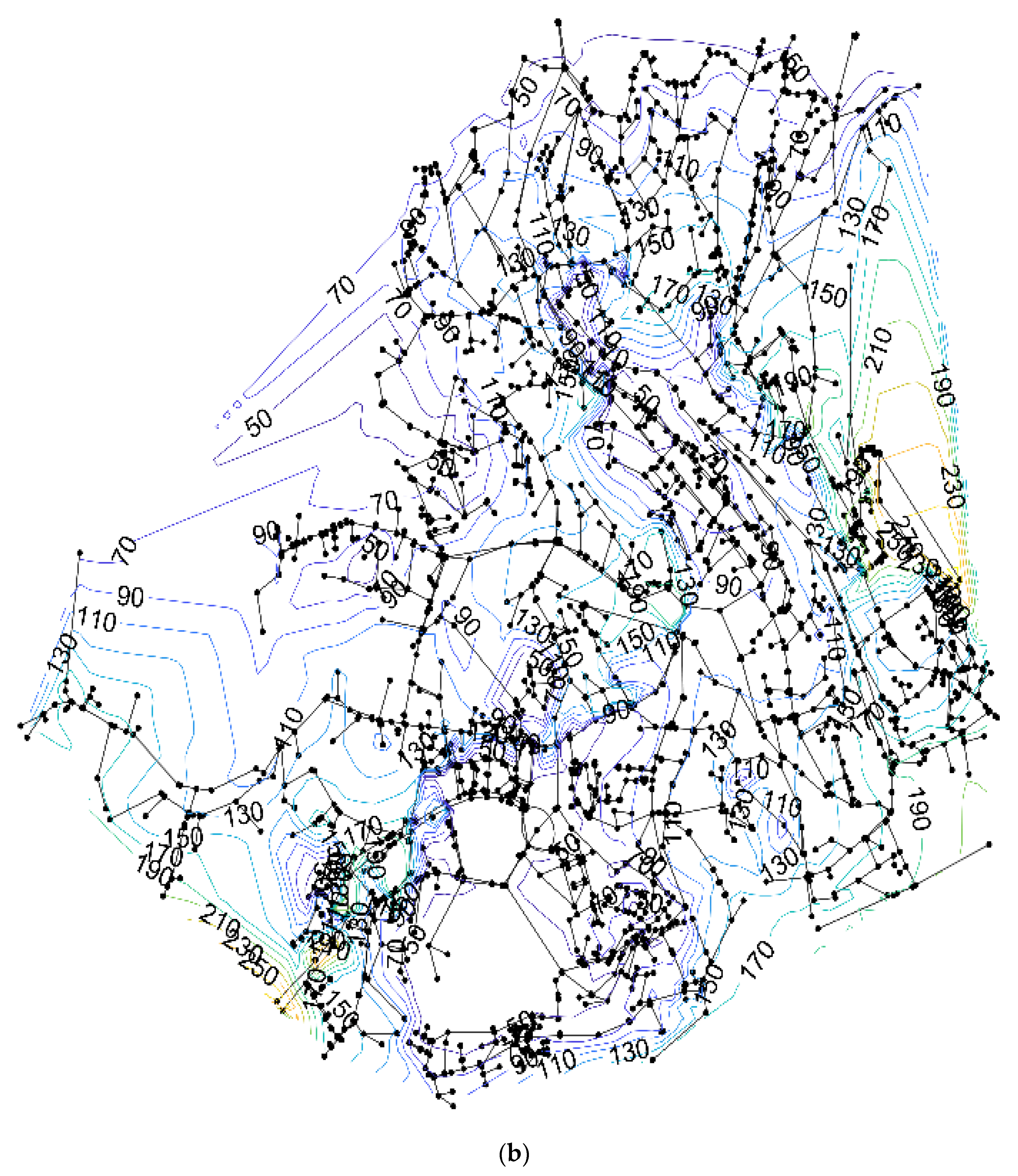
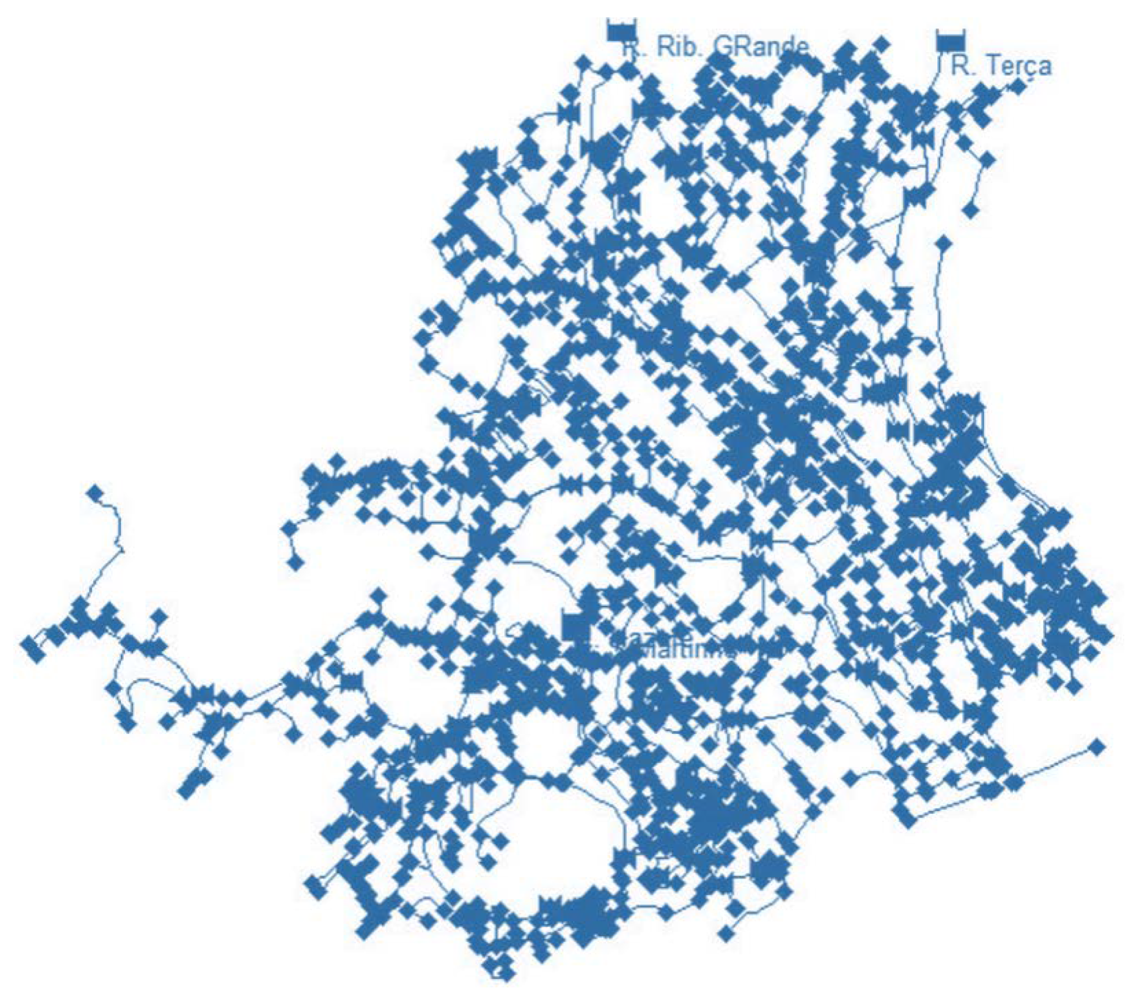
4. Application to the Water Distribution Network (WDN) of Funchal City—Madeira, Portugal

Once the design and performance of the novel turbine were investigated by experiments and CFD analyses, an application to a real case study network was then considered. The case study concerns the water distribution network supplying Funchal city in the Madeira region (PT) (Figure 11). Such a network consists of a number of links (l) and nodes ($\mathrm{n}$) as 2844 and 2801, respectively, and it is supplied by five reservoirs, whose water levels were assumed as constant. The total flowrate supplied by the reservoirs is 300 L/s. Out of five reservoirs, two are located at 360 and 400 m.a.s.l., whereas the elevation of the remaining three reservoirs is approximately 250 m.a.s.l. The network layout is presented in Figure 11. According to the current configuration of the network, several pressure reducing valves (PRVs) and throttle control valves (TCVs) are installed with the aim of controlling the pressure in the whole network. Moreover, further valves are present in order to close some links and determine a kind of district area of the network.

Due to the large topographical variability, a significant energy potential is available. Hence, the installation of one or more turbines could allow for a large production of energy, as well as a large water savings due to the reduction of the overall pressure. Nevertheless, in the links where the flow is significantly low, the energy production is low as well, and installing a valve instead of a turbine could be a more viable solution. Hence, in this study, the optimal location of turbines and valves was simultaneously investigated. An optimization procedure is implemented with reference to the daily average flow condition, with the aim of searching for the best scale design for turbines and, simultaneously, the best number and location of turbines and valves in order to maximize both water and energy savings, and minimize the investment cost.

4.1. The Optimization Procedure

In this study, the optimization problem was coupled with the hydraulic resolution of the network in one single mathematical model. Instead of using a hydraulic external solver (e.g., EPANET) to compute flow through links and pressure at nodes, the hydraulic behavior of the network is modeled within the optimization procedure by means of the mass continuity equations at the nodes and momentum balance equations along the pipes. The mathematical model will therefore consist of both linear and non-linear inequalities constraining the optimization problem, as well as non-linear equations modeling the hydraulic resolution of the network. With regard to the variables of the optimization, these are both binary (i.e., the installation of a device within a branch of the network) and continuous (i.e., pressure in the nodes, the discharges within the pipes, head loss within the devices). The resulting mathematical model is therefore a mixed integer non-linear programming (i.e., MINLP). Due to the non-convexity of some constraints, among the existing MINLP solvers, the Solving Constraint Integer Programs (SCIP) [45] was chosen to perform the optimization, since it is a robust global optimization solver, suitable for general MINLP problems—no matter if the optimization problem is convex or non-convex. SCIP relies on spatial branch-and-bound algorithm with linear relaxation, various heuristics, and bound-tightening procedures. This solver can handle only differentiable functions; hence, it cannot perform the optimization in the presence of absolute values, if/sign function, etc. Morani et al. (2021) [46,47] found proper formulations of both variables and constraints in a general optimal location problem, avoiding the use of any non-differentiable functions within the mathematical model. Most of these formulations will be used in this study and presented later on.

4.1.1. The Variables

The location of a general device within a water network consisting of $\mathrm{l}$ links and $\mathrm{n}$ nodes is represented by a binary variable (i.e., ${\mathrm{I}}_{\mathrm{k}}^{\mathrm{T}}$ and ${\mathrm{I}}_{\mathrm{k}}^{\mathrm{V}}$ for turbine and valve, respectively) assuming a value of 1 if the device is installed and 0 otherwise. As previously highlighted, since the hydraulic behavior of the network is modeled within the optimization procedure, flow through links (${\mathrm{Q}}_{\mathrm{k}}$) and head at nodes (${\mathrm{H}}_{\mathrm{i}}$) are continuous variables of the optimization problem. With regard to ${\mathrm{H}}_{\mathrm{i}}$, it is constrained between a lower and an upper bound, as follows:

$$\frac{{\mathrm{p}}_{\min }}{\mathsf{\gamma }}\le { \mathrm{H}}_{\mathrm{i}}-{ \mathrm{z}}_{\mathrm{i}} \le \frac{{\mathrm{p}}_{\max }}{\mathsf{\gamma }}$$

(8)

where ${\mathrm{p}}_{\min }$ and ${\mathrm{p}}_{\max }$ represent the minimum and maximum pressure values allowable at each node, ${\mathrm{z}}_{\mathrm{i}}$ the elevation of the $\mathrm{i}$-th ($\mathrm{i}=1\dots \mathrm{n}$) node, and $\mathsf{\gamma }$ the specific weight of water.

When the node is a reservoir ($\mathrm{r}$), the head ${\mathrm{H}}_{\mathrm{i}}\left(\mathrm{t}\right)$ is a boundary condition, and the variable is given by the discharge ${\mathrm{q}}_{\mathrm{r}}$, which flows into or out of the reservoir itself. Regarding the discharge (${\mathrm{Q}}_{\mathrm{k}}$) flowing through the $\mathrm{k}$-th ($\mathrm{k}=1\dots \mathrm{l}$) link, it is expressed according to Morani et al. (2021) [46], as follows:

$$0\le { \mathrm{q}}_{\mathrm{k}}^{+}\le { \mathrm{Q}}_{\max }{ \mathsf{\zeta }}_{\mathrm{k}}$$

(9)

$$0\le { \mathrm{q}}_{\mathrm{k}}^{-}\le { \mathrm{Q}}_{\max } \left(1-{ \mathsf{\zeta }}_{\mathrm{k}}\right)$$

(10)

where ${\mathrm{q}}_{\mathrm{k}}^{+}$ and ${\mathrm{q}}_{\mathrm{k}}^{-}$ are, respectively, the positive and negative parts of the discharge, and ${\mathrm{Q}}_{\max }$ is the upper bound. With regard to ${\mathsf{\zeta }}_{\mathrm{k}}$, it is a binary variable modeling the direction of the flow within a branch, and it is equal to 1 if the discharge flows according to the direction of the pipe $\mathrm{k}$ (i.e., the flow is given by the only positive component ${\mathrm{q}}_{\mathrm{k}}^{+}$) and 0 if otherwise (i.e., the flow is given by the only negative component ${\mathrm{q}}_{\mathrm{k}}^{-}$).

The head loss within the device (${\mathrm{H}}_{\mathrm{k}}^{\mathrm{T}}$ and ${\mathrm{H}}_{\mathrm{k}}^{\mathrm{V}}$ for turbine and valve, respectively) is a further continuous variable of the optimization problem. As presented in Morani et al. (2021) [46], these variables can also be split into their positive and negative components, as follows:

$$0\le { \mathrm{H}}_{\mathrm{k}}^{\mathrm{T}+} \le { \mathrm{H}}_{\mathrm{k} }{}_{\max }{ \mathsf{\zeta }}_{\mathrm{k}}$$

(11)

$$0\le { \mathrm{H}}_{\mathrm{k}}^{\mathrm{V}+} \le { \mathrm{H}}_{\mathrm{k} }{}_{\max }{ \mathsf{\zeta }}_{\mathrm{k}}$$

(12)

$$0\le { \mathrm{H}}_{\mathrm{k}}^{\mathrm{T}-} \le { \mathrm{H}}_{\mathrm{k} }{}_{\max } \left(1-{\mathsf{\zeta }}_{\mathrm{k}}\right)$$

(13)

$$0\le { \mathrm{H}}_{\mathrm{k}}^{\mathrm{V}-}\le { \mathrm{H}}_{\mathrm{k} }{}_{\max }\left(1-{ \mathsf{\zeta }}_{\mathrm{k}}\right)$$

(14)

where ${\mathrm{H}}_{\mathrm{k} }{}_{\max }$ is the maximum value of head loss achievable within the devices.

Further variables of the problem are related to the design of the turbines. The machine presented in the previous sections is a small-scale prototype; hence, its diameter (D) should be properly scaled to be suitable for such a real application. Such a diameter represents a further variable of the optimization problem and has is bounded as:

$$\mathrm{D}\ge { \mathrm{D}}_{\min }{ \mathrm{I}}_{\mathrm{k}}^{\mathrm{T}}$$

(15)

$$\mathrm{D}\le { \mathrm{D}}_{\max }{ \mathrm{I}}_{\mathrm{k}}^{\mathrm{T}}$$

(16)

where ${\mathrm{D}}_{\min }$ and ${\mathrm{D}}_{\max }$ represent the lower and upper bound, respectively, of the variable $\mathrm{D}$ in the case of turbine installation (i.e., ${\mathrm{I}}_{\mathrm{k}}^{\mathrm{T}}$ = 1).

A further design variable of the optimization problem is represented by the impeller thickness ($\mathsf{\alpha }$). As the diameter $\mathrm{D},\mathsf{\alpha }$ is constrained as:

$$\mathsf{\alpha }\ge { \mathsf{\alpha }}_{\min }{ \mathrm{I}}_{\mathrm{k}}^{\mathrm{T}}$$

(17)

$$\mathsf{\alpha }\le { \mathsf{\alpha }}_{\max }{ \mathrm{I}}_{\mathrm{k}}^{\mathrm{T}}$$

(18)

where ${\mathsf{\alpha }}_{\min }$ and ${\mathsf{\alpha }}_{\max }$ represent the lower and upper bound, respectively, of the variable $\mathsf{\alpha }$ in the presence of a turbine (i.e., ${\mathrm{I}}_{\mathrm{k}}^{\mathrm{T}}$ = 1).

4.1.2. Non-Linear Constraints

Most of the non-linearities in the optimization problem are given by the equations modeling the turbine design. In addition to the diameter ($\mathrm{D}$), the installed turbine should also be characterized in terms of flow (${\mathrm{Q}}_{\mathrm{T}}$), efficiency (${\mathsf{\eta }}_{\mathrm{T}}$) and producible power (${\mathrm{P}}_{\mathrm{T}}$). With regard to the flow through the turbine, it can be obtained from Equation (5), as follows:

$${\mathrm{Q}}_{\mathrm{T}}={ \mathrm{q}}_{\mathrm{T}}{ \mathrm{D}}^2 \mathsf{\alpha }\sqrt{\mathrm{g} \left({\mathrm{H}}_{\mathrm{k}}^{\mathrm{T}+}+{ \mathrm{H}}_{\mathrm{k}}^{\mathrm{T}-}\right)}$$

(19)

In order to set ${\mathrm{Q}}_{\mathrm{T}}$ as the total discharge flowing through the $\mathrm{k}$-th pipe if the turbine is installed, the following constraint was defined:

$${\mathrm{Q}}_{\mathrm{T}}=\left({\mathrm{q}}_{\mathrm{k}}^{+}+{ \mathrm{q}}_{\mathrm{k}}^{-}\right){ \mathrm{I}}_{\mathrm{k}}^{\mathrm{T}}$$

(20)

According to Equation (20), when the turbine is not installed in the $\mathrm{k}$-th pipe (i.e., ${\mathrm{I}}_{\mathrm{k}}^{\mathrm{T}}$ = 0), the ${\mathrm{Q}}_{\mathrm{T}}$ is forced to be equal to 0.

The turbine efficiency can be expressed according to Equation (7) as a function of (${\mathrm{H}}_{\mathrm{k}}^{\mathrm{T}+}+{ \mathrm{H}}_{\mathrm{k}}^{\mathrm{T}-}$):

$$\mathsf{\eta }=1-\left(0.4\right){\left(\frac{75}{1000 \mathrm{D}}\right)}^{0.25}{\left(\frac{5}{{\mathrm{H}}_{\mathrm{k}}^{\mathrm{T}+}+{ \mathrm{H}}_{\mathrm{k}}^{\mathrm{T}-}}\right)}^{0.1}$$

(21)

The producible power is hence given by the following expression:

$${\mathrm{P}}_{\mathrm{T}}=\mathsf{\gamma } \left({\mathrm{H}}_{\mathrm{k}}^{\mathrm{T}+}+{ \mathrm{H}}_{\mathrm{k}}^{\mathrm{T}-}\right){\mathrm{Q}}_{\mathrm{T} }\mathsf{\eta } {\mathsf{\eta }}_{\mathrm{G}}$$

(22)

where ${\mathsf{\eta }}_{\mathrm{G}}$ is the generator efficiency, assumed equal to 90%.

As constraints (19)–(22) are written with reference to each link of the network, the total number of such constraints is equal to $4\mathrm{l}$.

Further non-linearities are represented by the hydraulic equations modeling the resolution of the network, such as the mass continuity equations within the nodes, and momentum balance equations along the links.

Given a node $\mathrm{i}$ ($\mathrm{i}=1\dots \mathrm{n}$), the mass continuity equation can be expressed as follows:

$${\displaystyle \sum }_{\mathrm{k} \in { \mathrm{K}}_{\mathrm{i}}}{\left({\mathrm{q}}_{\mathrm{k}}^{+}+{ \mathrm{q}}_{\mathrm{k}}^{-}\right)}^{\mathrm{in}}-{\displaystyle \sum }_{\mathrm{k} \in { \mathrm{K}}_{\mathrm{i}}}{\left({\mathrm{q}}_{\mathrm{k}}^{+}+{ \mathrm{q}}_{\mathrm{k}}^{-}\right)}^{\mathrm{out}}-{ \mathrm{f}}_{\mathrm{i}} {({\mathrm{H}}_{\mathrm{i}}-{ \mathrm{z}}_{\mathrm{i}})}^{\mathsf{\beta }}={ \mathrm{q}}_{\mathrm{i}}^{\mathrm{d}}$$

(23)

where $\left({\mathrm{q}}_{\mathrm{k}}^{+}+{ \mathrm{q}}_{\mathrm{k}}^{-}\right)$ is the total discharge in the $\mathrm{k}$-th link belonging to set ${\mathrm{K}}_{\mathrm{i}}$ of links approaching the node $\mathrm{i}$, and the superscripts $\mathrm{in}$ and $\mathrm{out}$ indicate whether the discharge flows into or out of the $\mathrm{i}$-th node, respectively. The term ${\mathrm{f}}_{\mathrm{i}} {({\mathrm{H}}_{\mathrm{i}}-{ \mathrm{z}}_{\mathrm{i}})}^{\mathsf{\beta }}$ represents the amount of leaked water at the $\mathrm{i}$-th node, which will be better defined in Section 4.1.4. As the constraint (23) was written for each node $\mathrm{i}$ ($\mathrm{i}=1\dots \mathrm{n}$), the number of mass continuity equations can be accounted for as $\mathrm{n}$.

Given a link $\mathrm{k}$ ($\mathrm{k}=1\dots \mathrm{l}$), the momentum balance equation is given by the following expression:

$${\mathrm{H}}_{\mathrm{i}}-{ \mathrm{H}}_{\mathrm{j} }-{ \mathrm{r}}_{\mathrm{k}}{\mathrm{L}}_{\mathrm{k} }-({\mathrm{H}}_{\mathrm{k}}^{\mathrm{T}+}-{\mathrm{H}}_{\mathrm{k}}^{\mathrm{T}–})-({\mathrm{H}}_{\mathrm{k}}^{\mathrm{V}+}-{\mathrm{H}}_{\mathrm{k}}^{\mathrm{V}–})=0$$

(24)

where ${\mathrm{H}}_{\mathrm{i}}$ and ${\mathrm{H}}_{\mathrm{j}}$ are the head at the initial ($\mathrm{i}$-th) and final ($\mathrm{j}$-th) node of the $\mathrm{k}$-th link, and ${\mathrm{r}}_{\mathrm{k}}{\mathrm{L}}_{\mathrm{k} }$ is the head loss due to the resistance along the $\mathrm{k}$-th pipe presenting a length ${\mathrm{L}}_{\mathrm{k}}$. The unit head loss ${\mathrm{r}}_{\mathrm{k}}$ was calculated by the Hazen Williams formula:

$${\mathrm{r}}_{\mathrm{k}}=\frac{10.67}{{\mathrm{C}}_{\mathrm{k}}^{1.852}} \frac{\left[{({\mathrm{q}}_{\mathrm{k}}^{+})}^{1.852}-{({\mathrm{q}}_{\mathrm{k}}^{-})}^{1.852}\right]}{{\mathrm{D}}_{\mathrm{k}}^{4.8704}}$$

(25)

where ${\mathrm{C}}_{\mathrm{k}}$ and ${\mathrm{D}}_{\mathrm{k}}$ are the roughness coefficient and the diameter of the $\mathrm{k}$-th pipe, respectively. As constraint (24) is expressed for each link $\mathrm{k}$ ($\mathrm{k}=1\dots \mathrm{l}$), the total number of such constraints can be accounted for as $\mathrm{l}$.

4.1.3. Linear Constraints

Some linear constraints were used and were already presented in Section 4.1.1 (see Equations (9)–(14)) to define the variables of the problem. An additional set of $\mathrm{l}$ linear constraints (i.e., one for each link $\mathrm{k}$) was defined in order to avoid the installation of both turbine and valve within a same link:

$${\mathrm{I}}_{\mathrm{k}}^{\mathrm{T}}+{ \mathrm{I}}_{\mathrm{k}}^{\mathrm{V}} \le 1$$

(26)

Finally, further linear constraints were introduced in order to push the head loss within the devices to be equal to 0 if the device is not installed, and to be bounded otherwise.

$${\mathrm{H}}_{\mathrm{k} }^{\mathrm{T}+}+{\mathrm{H}}_{\mathrm{k} }^{\mathrm{T}-} \le {\mathrm{H}}_{\mathrm{k} }{}_{\max }{ \mathrm{I}}_{\mathrm{k}}^{\mathrm{T}}$$

(27)

$${\mathrm{H}}_{\mathrm{k} }^{\mathrm{V}+}+{\mathrm{H}}_{\mathrm{k} }^{\mathrm{V}-} \le {\mathrm{H}}_{\mathrm{k} }{}_{\max }{ \mathrm{I}}_{\mathrm{k}}^{\mathrm{V}}$$

(28)

As constraints (27) and (28) defined for each link $\mathrm{k}$ of the network, the total number of such devices is equal to $4\mathrm{l}$.

4.1.4. The Objective Function

As already highlighted, the aim of the optimization is to search for the best design and location of both turbines and valves, in order to maximize both the energy and water savings and minimize the investment cost. As in Morani et al. (2021) [46,48], the objective function that can be suitable for such an optimization problem is the net present value (NPV) of the investment, whose expression is given in Equation (29).

$$\mathrm{NPV}={\displaystyle \sum }_{\mathrm{k} =1}^{\mathrm{l}}\left(-{ \mathrm{c}}_{\mathrm{k}}^{\mathrm{T}}{ \mathrm{I}}_{\mathrm{k}}^{\mathrm{T}}-{ \mathrm{c}}_{\mathrm{k}}^{\mathrm{V}}{ \mathrm{I}}_{\mathrm{k}}^{\mathrm{V}}\right)+{\displaystyle \sum }_{\mathrm{y}=1}^{\mathrm{Y}}\frac{{\mathrm{E}}_{\mathrm{y}}^{\mathrm{p}}+{ \mathrm{W}}_{\mathrm{y}}^{\mathrm{s}} }{{\left(1+\mathsf{\lambda }\right)}^{\mathrm{y}}}$$

(29)

In Equation (29) the terms ${\mathrm{c}}_{\mathrm{k}}^{\mathrm{T}}{ \mathrm{I}}_{\mathrm{k}}^{\mathrm{T}}$ and ${\mathrm{c}}_{\mathrm{k}}^{\mathrm{V}}{ \mathrm{I}}_{\mathrm{k}}^{\mathrm{V}}$ represent, respectively, the total cost of turbines and valves occurring only at the beginning of the investment, whereas ${\mathrm{E}}_{\mathrm{y}}^{\mathrm{p}}$ and ${\mathrm{W}}_{\mathrm{y}}^{\mathrm{s}}$ are the annual inflow cash due, respectively, to the energy production and reduction of leaked water. Moreover, $\mathrm{Y}$ is the total number of $\mathrm{y}$ years, assumed as 10 years, and $\mathsf{\lambda }$ is the discount rate (set as 5%). In order to evaluate the annual income resulting from the energy production, an energy unit selling price equal to 0.1 €/kWh was assumed. With regard to the cost of the valve, the model cost suggested by Garcia et al. (2019) [49] was adopted, according to which the total cost of PRVs is dependent on pipe diameter (Figure 12):

With reference to the total cost of the turbines, since the analyzed turbine is a prototype, a function to properly model its cost is not actually available. Hence, in this study, the cost models of both a traditional turbine and a pump as turbine (PAT) (Figure 13) were alternatively used to carry out the optimization, since the effective cost model of the novel turbine is likely to comprise these two cost models. Among all the models presented in Figure 13, in this study the costs of the devices were evaluated according to the interpolations of experimental points presented by the authors in [50] (i.e., black dots for turbine unit costs and grey dots for PAT unit costs).

With regard to the annual income due to water saving (${\mathrm{W}}_{\mathrm{y}}^{\mathrm{s}}$) in Equation (29), it was evaluated as the difference between the total volume of water leaked without and in presence of devices within the network [46,48]:

$${\mathrm{W}}_{\mathrm{y}}^{\mathrm{s}}={ \mathrm{c}}_{\mathrm{w}} \left({\mathrm{Q}}_{\mathrm{l}}^0{\Delta \mathrm{t}}_{\mathrm{d}}-{\mathrm{Q}}_{\mathrm{l}}^{\mathrm{S}}\right)$$

(30)

The water unit cost ${\mathrm{c}}_{\mathrm{w}}$ was fixed as 0.3 €/m³, as representative of the analyzed case study area. According to the formulation proposed by Araujo et al. (2006) [55], the total leaked discharge in the network ${\mathrm{Q}}_{\mathrm{l}}$ can be evaluated as the sum of the discharge leaked in all single nodes:

$${\mathrm{Q}}_{\mathrm{l}}={\displaystyle \sum }_{\mathrm{i}=1}^{\mathrm{n}}{\mathrm{q}}_{\mathrm{i}}^{\mathrm{l}}={\displaystyle \sum }_{\mathrm{i}=1}^{\mathrm{n}}{\mathrm{f}}_{\mathrm{i} }{\left({\mathrm{H}}_{\mathrm{i}}-{\mathrm{z}}_{\mathrm{i}}\right)}^{\mathsf{\beta }}$$

(31)

where β is an exponent depending on both the material and the shape of the orifice [56], which was set equal to 1.18, according to Araujo et al. (2006) [48,55]. With regard to ${\mathrm{f}}_{\mathrm{i} }$, it represents a leakage coefficient whose expression is following presented:

$${\mathrm{f}}_{\mathrm{i} }= \mathrm{c}{\displaystyle \sum }_{\mathrm{j}=1}^{{\mathrm{K}}_{\mathrm{i}}}0.5{ \mathrm{L}}_{\mathrm{i},\mathrm{j}}$$

(32)

where $\mathrm{c}$ is a coefficient equal to $0.00001 \mathrm{L}/{\mathrm{s} \mathrm{m}}^{1+\mathsf{\beta }}$ [48,55] and ${\mathrm{K}}_{\mathrm{i}}$ is the set of nodes linked to the $\mathrm{i}$-th node by a pipe with length as ${\mathrm{L}}_{\mathrm{i},\mathrm{j}}$.

4.1.5. The Mathematical Model

The combination of all variables, objective function and linear/non-linear constraints presented in the previous sections results in the mathematical model in Equation (33).

Regarding the model in Equation (33), ${\mathrm{H}}_{\mathrm{k} }{}_{\max }$, that is the upper bound of the variables head losses within the devices, was set as 200 m; ${\mathrm{p}}_{\min }$ and ${\mathrm{p}}_{\max }$ were set as 25 m and 150 m, respectively. Regarding the bounds of the impeller diameter of the turbines, the lower bound ${\mathrm{D}}_{\min }$ was set as 50 mm, whereas the upper bound ${\mathrm{D}}_{\max }$ varies for each pipe $\mathrm{k}$ and is equal to four times the diameter of the pipe itself. Finally, the upper bound of the variable discharges, which is ${\mathrm{Q}}_{\max }$, was set as 500 L/s, whereas ${\mathsf{\alpha }}_{\min }$ and ${\mathsf{\alpha }}_{\max }$ were assumed equal at 10% and 200%, respectively.

As in Morani et al. (2021) [46], two small feasibility tolerances (${\mathrm{tol}}_{\mathrm{k}}^{\mathrm{H}}, {\mathrm{tol}}_{\mathrm{i}}^{\mathrm{Q}}$) were introduced within the momentum balance equation and mass continuity equation, respectively, in order to push the solver to achieve a solution. Such tolerances are small quantities (${\mathrm{tol}}_{\mathrm{k}}^{\mathrm{H}}$ = 0.01 m and ${\mathrm{tol}}_{\mathrm{i}}^{\mathrm{Q}}$ = 0.005 L/s) and can be considered as acceptable as all other uncertainties affecting the accuracy of the problem (e.g., evaluation of end-used demands, use of Hazen Williams formula).

$$\begin{gathered} \{\begin{array}{cc} \mathrm{maximize} \\ {\mathrm{I}}_{\mathrm{k}}^{\mathrm{T}},{\mathrm{I}}_{\mathrm{k}}^{\mathrm{V}},{\mathsf{\zeta }}_{\mathrm{k}} \\ {\mathrm{H}}_{\mathrm{k}}^{\mathrm{T}+},{\mathrm{H}}_{\mathrm{k} }^{\mathrm{T}-},{\mathrm{H}}_{\mathrm{k}}^{\mathrm{V}+},{\mathrm{H}}_{\mathrm{k} }^{\mathrm{V}-} \\ {\mathrm{q}}_{\mathrm{k}}^{+},{\mathrm{q}}_{\mathrm{k}}^{-},{\mathrm{H}}_{\mathrm{i}},\mathrm{D},\mathsf{\alpha },\hfill & \mathrm{NPV}={\displaystyle {\displaystyle \sum }_{\mathrm{k} =1}^{\mathrm{l}}}\left(-{ \mathrm{c}}_{\mathrm{k}}^{\mathrm{T}}{ \mathrm{I}}_{\mathrm{k}}^{\mathrm{T}}-{ \mathrm{c}}_{\mathrm{k}}^{\mathrm{V}}{ \mathrm{I}}_{\mathrm{k}}^{\mathrm{V}}\right)+{\displaystyle {\displaystyle \sum }_{\mathrm{y}=1}^{\mathrm{Y}}}\frac{{\mathrm{E}}_{\mathrm{y}}^{\mathrm{p}}+{ \mathrm{W}}_{\mathrm{y}}^{\mathrm{s}} }{{\left(1+\mathsf{\lambda }\right)}^{\mathrm{y}}}\\ -{\mathrm{tol}}_{\mathrm{i}}^{\mathrm{Q}}\le {\displaystyle {\displaystyle \sum }_{\mathrm{k} \in { \mathrm{K}}_{\mathrm{i}}}}{\left({\mathrm{q}}_{\mathrm{k}}^{+}+{ \mathrm{q}}_{\mathrm{k}}^{-}\right)}^{\mathrm{in}}-{\displaystyle {\displaystyle \sum }_{\mathrm{k} \in { \mathrm{K}}_{\mathrm{i}}}}{\left({\mathrm{q}}_{\mathrm{k}}^{+}+{ \mathrm{q}}_{\mathrm{k}}^{-}\right)}^{\mathrm{out}}-{ \mathrm{f}}_{\mathrm{i}}{ \mathrm{p}}_{\mathrm{i}}^{\mathsf{\beta }}-{ \mathrm{q}}_{\mathrm{i}}^{\mathrm{d}} \le { \mathrm{tol}}_{\mathrm{i}}^{\mathrm{Q}} \\ -{\mathrm{tol}}_{\mathrm{k}}^{\mathrm{H}}\le { \mathrm{H}}_{\mathrm{i}}-{ \mathrm{H}}_{\mathrm{j} }-{ \mathrm{r}}_{\mathrm{k}}{\mathrm{L}}_{\mathrm{k} }-({\mathrm{H}}_{\mathrm{k}}^{\mathrm{T}+}-{\mathrm{H}}_{\mathrm{k}}^{\mathrm{T}–})-({\mathrm{H}}_{\mathrm{k}}^{\mathrm{V}+}-{\mathrm{H}}_{\mathrm{k}}^{\mathrm{V}–})\le { \mathrm{tol}}_{\mathrm{k}}^{\mathrm{H}} \\ 0\le { \mathrm{q}}_{\mathrm{k}}^{+}\le { \mathrm{Q}}_{\max }{ \mathsf{\zeta }}_{\mathrm{k}} \\ 0 \le { \mathrm{q}}_{\mathrm{k}}^{-}\le { \mathrm{Q}}_{\max } \left(1-{\mathsf{\zeta }}_{\mathrm{k}}\right) \\ 0\le { \mathrm{H}}_{\mathrm{k}}^{\mathrm{T}+}\le { \mathrm{H}}_{\mathrm{k} }{}_{\max }{ \mathsf{\zeta }}_{\mathrm{k}} \\ 0\le { \mathrm{H}}_{\mathrm{k}}^{\mathrm{T}-}\le { \mathrm{H}}_{\mathrm{k} }{}_{\max } \left(1-{ \mathsf{\zeta }}_{\mathrm{k}}\right) \\ 0\le { \mathrm{H}}_{\mathrm{k}}^{\mathrm{V}+}\le { \mathrm{H}}_{\mathrm{k} }{}_{\max }{ \mathsf{\zeta }}_{\mathrm{k}} \\ 0\le { \mathrm{H}}_{\mathrm{k}}^{\mathrm{V}-}\le { \mathrm{H}}_{\mathrm{k} }{}_{\max } \left(1-{ \mathsf{\zeta }}_{\mathrm{k}}\right) \\ \mathrm{D}\ge { \mathrm{D}}_{\min }{ \mathrm{I}}_{\mathrm{k}}^{\mathrm{T}} \\ \mathrm{D}\le { \mathrm{D}}_{\max }{ \mathrm{I}}_{\mathrm{k}}^{\mathrm{T}} \\ \mathsf{\alpha }\ge { \mathsf{\alpha }}_{\min }{ \mathrm{I}}_{\mathrm{k}}^{\mathrm{T}} \\ \mathsf{\alpha }\le { \mathsf{\alpha }}_{\max }{ \mathrm{I}}_{\mathrm{k}}^{\mathrm{T}} \\ {\mathrm{Q}}_{\mathrm{T}}={ \mathrm{q}}_{\mathrm{T}}{ \mathrm{D}}^2 \mathsf{\alpha }\sqrt{\mathrm{g} \left({\mathrm{H}}_{\mathrm{k}}^{\mathrm{T}+}+{ \mathrm{H}}_{\mathrm{k}}^{\mathrm{T}-}\right)}\\ \mathrm{subject} \mathrm{to}\hfill & \\ & \mathsf{\eta }=1-\left(0.4\right){\left(\frac{75}{1000 \mathrm{D}}\right)}^{0.25}{\left(\frac{5}{{\mathrm{H}}_{\mathrm{k}}^{\mathrm{T}+}+{ \mathrm{H}}_{\mathrm{k}}^{\mathrm{T}-}}\right)}^{0.1} \\ {\mathrm{P}}_{\mathrm{T}}=\mathsf{\gamma } \left({\mathrm{H}}_{\mathrm{k}}^{\mathrm{T}+}+{ \mathrm{H}}_{\mathrm{k}}^{\mathrm{T}-}\right){\mathrm{Q}}_{\mathrm{T}}{ \mathsf{\eta }}_{ }{\mathsf{\eta }}_{\mathrm{G}} \\ \frac{{\mathrm{p}}_{\min }}{\mathsf{\gamma }}\le \left({\mathrm{H}}_{\mathrm{i}}-{ \mathrm{z}}_{\mathrm{i}}\right)\le \frac{{\mathrm{p}}_{\max }}{\mathsf{\gamma }} \\ {\mathrm{H}}_{\mathrm{k} }^{\mathrm{T}+}+{\mathrm{H}}_{\mathrm{k} }^{\mathrm{T}-} \le {\mathrm{H}}_{\mathrm{k} }{}_{\max }{ \mathrm{I}}_{\mathrm{k}}^{\mathrm{T}} \\ {\mathrm{H}}_{\mathrm{k} }^{\mathrm{V}+}+{\mathrm{H}}_{\mathrm{k} }^{\mathrm{V}-} \le {\mathrm{H}}_{\mathrm{k} }{}_{\max }{ \mathrm{I}}_{\mathrm{k}}^{\mathrm{V}} \\ {\mathrm{Q}}_{\mathrm{T}}=\left({\mathrm{q}}_{\mathrm{k}}^{+}+{ \mathrm{q}}_{\mathrm{k}}^{-}\right){ \mathrm{I}}_{\mathrm{k}}^{\mathrm{T}} \\ {\mathrm{I}}_{\mathrm{k}}^{\mathrm{T}}+{ \mathrm{I}}_{\mathrm{k}}^{\mathrm{V}} \le 1 \\ 0\le { \mathrm{I}}_{\mathrm{k}}^{\mathrm{T}}\le 1 \\ 0\le { \mathrm{I}}_{\mathrm{k}}^{\mathrm{V}}\le 1 \\ 0\le { \mathsf{\zeta }}_{\mathrm{k}}\le 1 \\ ({\mathrm{I}}_{\mathrm{k}}^{\mathrm{T}},{ \mathrm{I}}_{\mathrm{k}}^{\mathrm{v}},{\mathsf{\zeta }}_{\mathrm{k}})\in \mathbb{Z} \left({\mathrm{H}}_{\mathrm{k}}^{\mathrm{T}+},{\mathrm{H}}_{\mathrm{k}}^{\mathrm{T}-},{ \mathrm{H}}_{\mathrm{k}}^{\mathrm{V}+},{\mathrm{H}}_{\mathrm{k}}^{\mathrm{V}-}\right) \in ℝ, \\ \left({\mathrm{q}}_{\mathrm{k}}^{+},{\mathrm{q}}_{\mathrm{k}}^{-},{\mathrm{Q}}_{\mathrm{T}},{\mathrm{P}}_{\mathrm{T}},{ \mathsf{\eta }}_{\mathrm{T}}, \mathrm{D}, \mathsf{\alpha }\right) \in ℝ \\ \forall \mathrm{i},\mathrm{j}=1\dots \mathrm{n},\hspace{1em}\hspace{1em}\forall \mathrm{k}=1\dots \mathrm{l} \end{array} \end{gathered}$$

(33)

The total number of variables amounts to 42,617, whereas the sum of both linear and non-linear constraints is accounted for as 51,149.

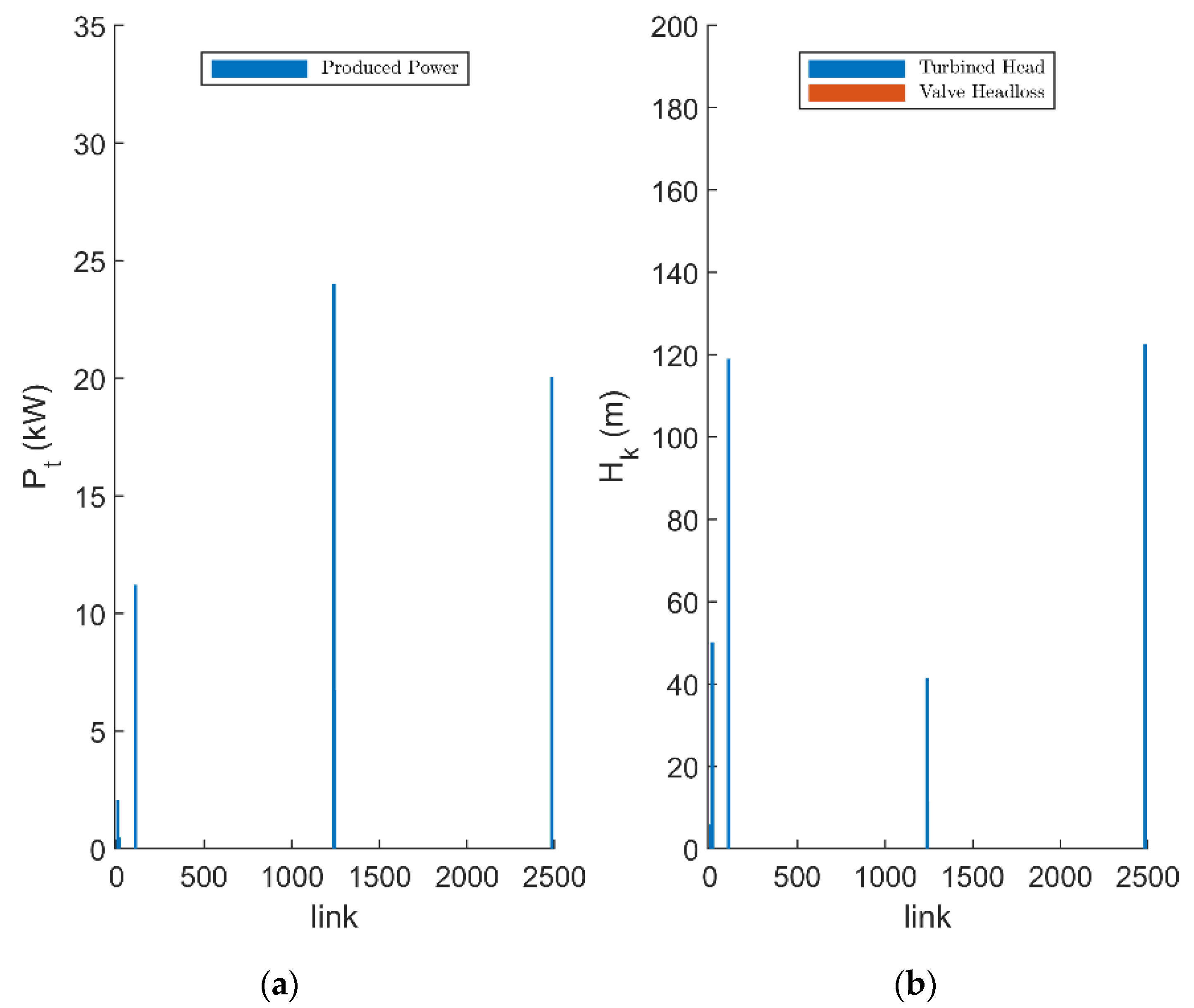
4.2. Optimization Results

Table 2. Results of the optimization procedure using two different literature cost models.

	NPV (€)	N° Turbines (-)	N° Valves (-)	Av. Power (kW)	Water Saving (m3/day)	Invest. Cost (€)
(I) 1	7,169,083	5	4	68	8507	482,298
(II) 1	11,942,920	6	1	65	13,673	55,786

¹ (I): traditional turbine + generator cost model; (II) PAT + generator cost model.

shows the results of the optimization obtained by using the cost models presented in Section 4.1.4. In Table 2, (I) and (II) refer to results obtained when a traditional turbine and a PAT cost model, respectively, are employed to evaluate the cost of the installed turbines.

When the turbine cost is evaluated according to the traditional turbine cost model (see (I)), the optimization solver installs a number of turbines and valves as 5 and 4, respectively, with an investment cost of EUR 482,298.

The resulting average produced power was accounted for as 68 kW, and the amount of water saved per day is equal to 8507 m³. When the literature PAT cost model is, instead, employed to evaluate the cost of the installed turbines (see (II)), the solver selects more turbines than valves (i.e., 6 against 1—Figure 14), since the installation of valves could not be convenient compared to turbines, especially where the pipe diameters are large. However, compared to the results in case (I), the increased value of NPV in case (II) (i.e., EUR 11,942,920) is due to the larger water savings, which is equal to 13,673 m³ per day, and smaller investment costs (EUR 55,786). Regarding the power production, it is quite similar between the two cases, obtaining around 65 kW.

The turbines are installed in both the cases in the middle region of the network, whereas the valves are installed in the peripheral area, where the water saving potential is large but the recoverable energy is contained.

Table 3. Turbine geometry resulting from case (I).

	D (mm)	HT (m)	QT (L/s)	N (rpm)	ηT (%)
Link 89	187	52	11	2748	75
Link 795	540	50	91	933	81
Link 1358	500	5	25	319	75
Link 1375	940	13.5	144	278	80
Link 2485	165	161	15	5480	77

and

Table 4. Turbine geometry resulting from case (II).

	D (mm)	HT (m)	QT (L/s)	N (rpm)	ηT (%)
Link 8	685	5.95	51	254	77
Link 14	70	50	1.6	7200	68
Link 108	170	119	14	4573	76
Link 1241	535	41.5	82	858	80
Link 1242	747	11.5	84	323	79
Link 2485	220	122.5	24	3585	78

show the results in terms of turbine geometry and operating conditions at BEP for case (I) and case (II), respectively. With reference to $\mathrm{N}$, it is the rotational speed resulting from the optimal diameter ($\mathrm{D}$) and head drop (${\mathrm{H}}_{\mathrm{T}}$) according to Equation (6).

Figure 15a shows the pressure contour plots according to case (I) when devices are installed within the network: the installation results in a significant reduction in the overall excess pressure when compared with the scenario without installed devices (Figure 15b). The same is valid for case (II), whose pressure contour plot is presented in Appendix A (Figure A1).

The produced power, as well as the head drop within the installed devices, for case (I) is shown in Figure 16a,b, respectively. According to Figure 16b, the reduction in head resulting from the device installation is significant, even reaching a value of 160 m. The same figure for case (II) is presented in Appendix A (Figure A2).

5. Conclusions

In this paper a new centrifugal micro-turbine (CMT) was investigated in terms of performance and design. Based on a CFD modeling coupled with experimental tests on a turbine prototype, the unstable phenomena affecting the turbine components during its operation have been investigated in detail. In particular, the velocity and pressure profiles within turbine components were presented for different operating conditions. According to the results, the difference in terms of pressure drop at inlet and outlet of the rotor is significantly small, except for rotational speeds greater than 1850 rpm. According to the velocity profiles at the runners, high flow acceleration was detected from the leading edge to the trailing edge, followed by a significant flow deceleration due to an increase in static pressure. Moreover, the degree of flow deceleration was lower for high rotational speeds, at which the internal losses were therefore lower. A maximum velocity value of 12 m/s was detected in the region close to the leading edge of the rotating blade, whereas the minimum velocity of around 1 m/s is presented at the right side of the vane. However, the validation of the CFD numerical simulation was proven by a good agreement with experimental data in terms of global parameters. Based on affinity laws and the experimental tests, some relationships were obtained to design the centrifugal turbine at its best efficiency point. Finally, based on this new centrifugal micro-turbine design, a real water distribution network (WDN), in the Funchal system, was assumed as the case study and an optimization procedure was carried out in order to search for an optimal scale design of turbines, as well as an optimal location of such designed turbines together with pressure reducing valves (PRV), in order to maximize the energy production and minimize the leakage water volume. Due to the lack of information about the purchase cost of such a new centrifugal turbine, two different literature cost models were assumed to evaluate the investment cost: the effective solution will definitely comprise the two obtained solutions. According to the results, the use of a PAT cost model pushes the solver to install more turbines than valves. Moreover, compared to the solution resulting from the use of a traditional turbine cost model, when the turbine cost is evaluated according to a literature PAT cost model, the resulting water savings is large (i.e., 13,673 m³ per day against 8507 m³ per day) and the investment cost is significantly more confined (EUR 55,786 against EUR 482,298), where the power production has been accounted for at around 65 kW. However, in both analyzed cases, the turbines are installed in the middle part of the network, where the available energy is significant, whereas the valves are mainly located in the peripheral area where valves represent a more viable solution due to the limited available potential energy.

References

1. Zhu, D.; Tao, R.; Xiao, R.; Pan, L. Solving the runner blade crack problem for a Francis hydro-turbine operating under condition-complexity. Renew. Energy 2020, 149, 298–320. [Google Scholar] [CrossRef]
2. Morani, M.C.; Carravetta, A.; Del Giudice, G.; McNabola, A.; Fecarotta, O. A Comparison of Energy Recovery by PATs against Direct Variable Speed Pumping in Water Distribution Networks. Fluids 2018, 3, 41. [Google Scholar] [CrossRef] [Green Version]
3. Carravetta, A.; Del Giudice, G.; Fecarotta, O.; Gallagher, J.; Morani, M.C.; Ramos, H.M. The Potential Energy, Economic & Environmental Impacts of Hydro Power Pressure Reduction on the Water-Energy-Food Nexus. J. Water Resour. Plan. Manag. 2022, accepted. [Google Scholar]
4. Pasche, S.; Gallaire, F.; Avellan, F. Origin of the synchronous pressure fluctuations in the draft tube of Francis turbines operating at part load conditions. J. Fluids Struct. 2019, 86, 13–33. [Google Scholar] [CrossRef]
5. Morani, M.C.; Carravetta, A.; Fecarotta, O.; McNabola, A. Energy transfer from the freshwater to the wastewater network using a PAT-equipped turbopump. Water 2020, 12, 38. [Google Scholar] [CrossRef] [Green Version]
6. Thapa, B.S.; Dahlhaug, O.G.; Thapa, B. Flow measurements around guide vanes of Francis turbine: A PIV approach. Renew. Energy 2018, 126, 177–188. [Google Scholar] [CrossRef]
7. Gautam, S.; Neopane, H.P.; Acharya, N.; Chitrakar, S.; Thapa, B.S.; Zhu, B. Sediment erosion in low specific speed francis turbines: A case study on effects and causes. Wear 2020, 442-443, 203152. [Google Scholar] [CrossRef]
8. Tiwari, G.; Kumar, J.; Prasad, V.; Patel, V.K. Utility of CFD in the design and performance analysis of hydraulic turbines—A review. Energy Rep. 2020, 6, 2410–2429. [Google Scholar] [CrossRef]
9. Trivedi, C.; Gandhi, B.; Michel, C.J. Effect of transients on Francis turbine runner life: A review. J. Hydraul. Res. 2013, 51, 121–132. [Google Scholar] [CrossRef]
10. Goyal, R.; Gandhi, B.K. Review of hydrodynamics instabilities in Francis turbine during off-design and transient operations. Renew. Energy 2018, 116, 697–709. [Google Scholar] [CrossRef]
11. Nicolet, C. Hydroacoustic modelling and numerical simulation of unsteady operation of hydroelectric systems. Ec. Polytech. Fédérale Lausanne 2017. [Google Scholar] [CrossRef]
12. Goyal, R.; Trivedi, C.; Gandhi, B.K.; Cervantes, M. Numerical Simulation and Validation of a High Head Model Francis Turbine at Part Load Operating Condition. J. Inst. Eng. (India) Ser. C 2018, 99, 557–570. [Google Scholar] [CrossRef]
13. Bergan, C.; Goyal, R.; Cervantes, M.J.; Dahlhaug, O.G. Experimental Investigation of a High Head Model Francis Turbine During Steady-State Operation at Off-Design Conditions. In IOP Conference Series: Earth and Environmental Science; IOP Publishing: Bristol, UK, 2016. [Google Scholar]
14. Trivedi, C.; Cervantes, M.J.; Gandhi, B.K.; Dahlhaug, O.G. Experimental and numerical studies for a high head Francis turbine at several operating points. J. Fluids Eng. Trans. ASME 2013, 135, 111102. [Google Scholar] [CrossRef]
15. Zhang, F.; Lowys, P.; Houdeline, J.; Guo, X.; Hong, P.; Laurant, Y. Pump-turbine Rotor-Stator Interaction Induced Vibration: Problem Resolution and Experience. In IOP Conference Series: Earth and Environmental Science; IOP Publishing: Bristol, UK, 2021. [Google Scholar]
16. Keck, H.; Sick, M. Thirty years of numerical flow simulation in hydraulic turbomachines. Acta Mech. 2008, 201, 211–229. [Google Scholar] [CrossRef]
17. Favrel, A.; Junior, J.G.P.; Landry, C.; Müller, A.; Yamaishi, K.; Avellan, F. Dynamic modal analysis during reduced scale model tests of hydraulic turbines for hydro-acoustic characterization of cavitation flows. Mech. Syst. Signal Process. 2019, 117, 81–96. [Google Scholar] [CrossRef]
18. Scarlett, G.T.; Viola, I.M. Unsteady hydrodynamics of tidal turbine blades. Renew. Energy 2020, 146, 843–855. [Google Scholar] [CrossRef]
19. Luna-Ramírez, A.; Campos-Amezcua, A.; Dorantes-Gómez, O.; Mazur-Czerwiec, Z.; Muñoz-Quezada, R. Failure analysis of runner blades in a Francis hydraulic turbine—Case study. Eng. Fail. Anal. 2016, 59, 314–325. [Google Scholar] [CrossRef]
20. Khare, R.; Prasad, V.; Kumar, S. Cfd Approach for Flow Characteristics of Hydraulic Francis Turbine. Int. J. Eng. Sci. 2010, 2, 3824–3831. [Google Scholar]
21. Tiwari, G.; Prasad, V.; Shukla, S.; Patel, V.K. Hydrodynamic analysis of a low head prototype Francis turbine for establishing an optimum operating regime using CFD. J. Mech. Eng. Sci. 2020, 14, 6625–6641. [Google Scholar] [CrossRef]
22. Kerikous, E.; Thévenin, D. Optimal shape of thick blades for a hydraulic Savonius turbine. Renew. Energy 2019, 134, 629–638. [Google Scholar] [CrossRef]
23. Ma, Z.; Zhu, B.; Rao, C.; Shangguan, Y. Comprehensive Hydraulic Improvement and Parametric Analysis of a Francis Turbine Runner. Energies 2019, 12, 307. [Google Scholar] [CrossRef] [Green Version]
24. Pérez, L.C.A.; Acosta, M.J.A.; Yepes, C.A.P. CFD simulation data of a pico-hydro turbine. Data Brief 2020, 33, 106596. [Google Scholar] [CrossRef] [PubMed]
25. Chen, J.; Engeda, A. Standard module hydraulic technology: A novel geometrical design methodology and analysis for a low-head hydraulic turbine system, Part I: General design methodology and basic geometry considerations. Energy 2020, 196, 117151. [Google Scholar] [CrossRef]
26. Bai, B.; Zhang, L.; Guo, T.; Liu, C. Analysis of Dynamic Characteristics of the Main Shaft System in a Hydro-turbine Based on ANSYS. Procedia Eng. 2012, 31, 654–658. [Google Scholar] [CrossRef] [Green Version]
27. Tog, R.A.; Tousi, A.; Tourani, A. Comparison of turbulence methods in CFD analysis of compressible flows in radial turbomachines. Aircr. Eng. Aerosp. Technol. 2008, 80, 657–665. [Google Scholar]
28. Fluent, A. Ansys Fluent Theory Guide; ANSYS Inc.: Canonsburg, PA, USA, 2013. [Google Scholar]
29. Chen, B.; Yuan, X. Advanced Aerodynamic Optimization System for Turbomachinery. J. Turbomach. 2008, 130, 021005. [Google Scholar] [CrossRef]
30. Biesinger, T.; Cornelius, C.; Rube, C.; Braune, A.; Campregher, R.; Godin, P.G.; Schmid, G.; Zori, L. Unsteady CFD Methods in a Commercial Solver for Turbomachinery Applications. In Proceedings of the ASME Turbo Expo 2010: Power for Land, Sea, and Air, Glasgow, UK, 14–18 June 2010; pp. 2441–2452. [Google Scholar]
31. Wang, J.-F.; Piechna, J.; Müller, N. A Novel Design of Composite Water Turbine Using CFD. J. Hydrodyn. 2012, 24, 11–16. [Google Scholar] [CrossRef]
32. González, J.; Oro, J.M.F.; Argüelles-Díaz, K.M.; Santolaria, C. Flow analysis for a double suction centrifugal machine in the pump and turbine operation modes. Int. J. Numer. Methods Fluids 2009, 61, 220–236. [Google Scholar] [CrossRef]
33. Bogdanović-Jovanović, J.B.; Milenković, D.R.; Svrkota, D.M.; Bogdanović, B.; Spasić, Z.T. Pumps used as turbines: Power recovery, energy efficiency, CFD analysis. Therm. Sci. 2014, 18, 1029–1040. [Google Scholar] [CrossRef]
34. Fecarotta, O.; Messa, G.V.; Pugliese, F. Numerical assessment of the vulnerability to impact erosion of a pump as turbine in a water supply system. J. Hydroinformatics 2020, 22, 691–712. [Google Scholar]
35. Morros, C.S.; Oro, J.M.F.; Díaz, K.M.A. Numerical modelling and flow analysis of a centrifugal pump running as a turbine: Unsteady flow structures and its effects on the global performance. Int. J. Numer. Methods Fluids 2011, 65, 542–562. [Google Scholar] [CrossRef]
36. Barrio, R.M.; Fernández, J.; Blanco, E.F.; Parrondo, J.L.; Marcos, A. Performance characteristics and internal flow patterns in a reverse-running pump–turbine. Proc. Inst. Mech. Eng. Part C J. Mech. Eng. Sci. 2011, 226, 695–708. [Google Scholar] [CrossRef]
37. Dickinson, E.; Ekström, H.; Fontes, E. COMSOL Multiphysics. Electrochem. Commun. 2014, 40, 71–74. [Google Scholar] [CrossRef]
38. Georgescu, A.-M.; Georgescu, S.-C.; Bernad, S.I.; Cosoiu, C.I. Comsol Multiphysics versus Fluent: 2D Numerical Simuation of the Stationary Flow around a Blade of the Achard Turbine. Sci. Bull. Politeh. Univ. Timis. Trans. Mech. 2007, 52, 13–21. [Google Scholar]
39. AutoCAD Basics. In Construction Detailing for Interior Design. 2020. Available online: https://www.autodesk.it (accessed on 25 December 2021).
40. Simão, M.; Mora-Rodriguez, J.; Ramos, H. Computational dynamic models and experiments in the fluid–structure interaction of pipe systems. Can. J. Civ. Eng. 2016, 43, 60–72. [Google Scholar] [CrossRef]
41. Speziale, C.G. On nonlinear K-l and K-ε models of turbulence. J. Fluid Mech. 1987, 178, 459–475. [Google Scholar] [CrossRef]
42. Gresho, P. Incompressible Fluid Dynamics: Some Fundamental Formulation Issues. Annu. Rev. Fluid Mech. 1991, 23, 413–453. [Google Scholar] [CrossRef]
43. Simão, M.; Besharat, M.; Carravetta, A.; Ramos, H.M. Flow Velocity Distribution Towards Flowmeter Accuracy: CFD, UDV, and Field Tests. Water 2018, 10, 1807. [Google Scholar] [CrossRef] [Green Version]
44. Yang, J.; Preidikman, S.; Balaras, E. A Strong Coupling Scheme for Fluid-Structure Interaction Problems in Viscous Incompressible Flows. In Proceedings of the International Conference on Computational Methods for Coupled Problems in Science and Engineering, Santorini Island, Greece, 25–28 May 2005. [Google Scholar]
45. Vigerske, S.; Gleixner, A. SCIP: Global optimization of mixed-integer nonlinear programs in a branch-and-cut framework. Optim. Methods Softw. 2018, 33, 563–593. [Google Scholar] [CrossRef]
46. Morani, M.C.; Carravetta, A.; D’ambrosio, C.; Fecarotta, O. A new mixed integer non-linear programming model for optimal PAT and PRV location in water distribution networks. Urban Water J. 2021, 18, 394–409. [Google Scholar] [CrossRef]
47. Morani, M.C.; Carravetta, A.; D’ambrosio, C.; Fecarotta, O. A New Preliminary Model to Optimize PATs Location in a Water Distribution Network. Environ. Sci. Proc. 2020, 2, 57. [Google Scholar] [CrossRef]
48. Fecarotta, O.; McNabola, A. Optimal Location of Pump as Turbines (PATs) in Water Distribution Networks to Recover Energy and Reduce Leakage. Water Resour. Manag. 2017, 31, 5043–5059. [Google Scholar] [CrossRef]
49. García, J.M.; Salcedo, C.; Saldarriaga, J. Minimization of Water Losses in WDS through the Optimal Location of Valves and Turbines: A Comparison between Methodologies. In Proceedings of the World Environmental and Water Resources Congress 2019: Hydraulics, Waterways, and Water Distribu-tion Systems Analysis—Selected Papers from the World Environmental and Water Resources Congress 2019, Pittsburgh, PA, USA, 19–23 May 2019. [Google Scholar] [CrossRef]
50. Novara, D.; Carravetta, A.; McNabola, A.; Ramos, H.M. Cost Model for Pumps as Turbines in Run-of-River and In-Pipe Microhydropower Applications. J. Water Resour. Plan. Manag. 2019, 145, 04019012. [Google Scholar] [CrossRef]
51. De Marchis, M.; Fontanazza, C.M.; Freni, G.; Messineo, A.; Milici, B.; Napoli, E.; Notaro, V.; Puleo, V.; Scopa, A. Energy recovery in water distribution networks. Implementation of pumps as turbine in a dynamic numerical model. Procedia Eng. 2014, 70, 439–448. [Google Scholar] [CrossRef] [Green Version]
52. Carravetta, A.; Del Giudice, G.; Fecarotta, O.; Ramos, H. PAT Design Strategy for Energy Recovery in Water Distribution Networks by Electrical Regulation. Energies 2013, 6, 411–424. [Google Scholar] [CrossRef] [Green Version]
53. Ramos, H.M.; Borga, A.; Simão, M. New design solutions for low-power energy production in water pipe systems. Water Sci. Eng. 2009, 2, 69–84. [Google Scholar]
54. Ogayar, B.; Vidal, P.G. Cost determination of the electro-mechanical equipment of a small hydro-power plant. Renew. Energy 2009, 34, 6–13. [Google Scholar] [CrossRef]
55. Araujo, L.S.; Ramos, H.M.; Coelho, S.T. Pressure Control for Leakage Minimisation inWater Distribution Systems Management. Water Resour. Manag. 2006, 20, 133–149. [Google Scholar] [CrossRef]
56. Greyvenstein, B.; Van Zyl, J.E. An experimental investigation into the pressure—Leakage relationship of some failed water pipes. J. Water Supply Res. Technol. Aqua 2007, 56, 117–124. [Google Scholar] [CrossRef]
Figure 1. Experimental setup of the centrifugal turbine. Units: mm.
Energies 15 01528 g001
Figure 2. Turbine prototype: (a) description; (b,c) dimensions. Units: mm.
Energies 15 01528 g002
Figure 3. Pressure contours for different rotational speeds: (a) N = 750 rpm; (b) N = 1050 rpm; (c) N = 1500 rpm; (d) N = 1600 rpm; (e) N = 1800 rpm; (f) N = 1850 rpm.
Energies 15 01528 g003
Figure 4. Comparison in terms of total pressure drop between inlet and outlet rotor.
Energies 15 01528 g004
Figure 5. Velocity isosurfaces in the turbine runner for different rotational speeds: (a) N = 750 rpm; (b) N = 1050 rpm; (c) N = 1500 rpm; (d) N = 1600 rpm; (e) N = 1800 rpm; (f) N = 1850 rpm.
Energies 15 01528 g005
Figure 6. Velocity isosurface in the runner and draft tube for different rotational speeds with H = 32.8 m: (a) N = 750 rpm; (b) N = 1050 rpm; (c) N = 1500 rpm; (d) N = 1600; (e) N = 1800 rpm; (f) N = 1850 rpm.
Energies 15 01528 g006
Figure 7. Velocity magnitude for H = 32.8m and different rotational speeds: (a) N = 750 rpm; (b) N = 1050 rpm; (c) N = 1500 rpm; (d) N = 1600; (e) N = 1800 rpm; (f) N = 1850 rpm; (g) general horizontal plan view.
Energies 15 01528 g007
Figure 8. Velocity streamlines near the impeller for different rotational speeds: (a) N = 750 rpm; (b) N = 1050 rpm; (c) N = 1500 rpm; (d) N = 1600; (e) N = 1800 rpm; (f) N = 1850 rpm.
Energies 15 01528 g008
Figure 9. Detail of velocity streamlines with reference to the top view (a) and bottom view (b) of the guide vane (N = 1500 rpm).
Energies 15 01528 g009
Figure 10. Comparison between experimental measurements and numerical results. (a) Efficiency vs. flow rate coefficient; (b) torque coefficient vs. flow rate coefficient; (c) head coefficient vs flow rate coefficient.
Energies 15 01528 g010
Figure 11. Funchal network layout.
Energies 15 01528 g011
Figure 12. Total PRV cost depending on pipe diameter according to Garcia et al. (2019) [49].
Energies 15 01528 g012
Figure 13. Unit cost per rated power of PATs and conventional turbines coupled to generators [50], compared to other literature cost models [51,52,53,54].
Energies 15 01528 g013
Figure 14. Device positions within the case study WDN according to the results in (I) (a) and (II) (b).
Energies 15 01528 g014
Figure 15. Pressure contour plot when devices are installed (a) and without performing any pressure control strategy (b) for case (I).
Energies 15 01528 g015
Figure 16. Produced power of the installed turbines (a) and head drop within the devices (b) resulting from case (I).
Energies 15 01528 g016