1. Introduction
In recent years, interest in cybersecurity issues has grown significantly due to Industry 4.0 [
1,
2,
3] and IoT [
4,
5], autonomous cars, autonomous vacuum cleaners, and the development of “smart” devices that often cooperate or communicate with other surrounding devices. The convenience of using modern technology and the possibility to constantly monitor devices from anywhere over the Internet also brings new threats, namely by opening the door to other network users. With insufficient security measures in place, adversaries are able to establish steganographic command and control channels, eavesdrop on transmitted content, modify it, or even take control of the controlled device. It is especially dangerous in industrial networks (SCADA; supervisory control and data acquisition), which are used to control huge technological installations including critical infrastructure (power industry, petrochemical plants, transmission networks, etc.) [
6].
Communication in industrial networks differs from communication in IT networks [
7,
8]. Communication in industrial networks is based on protocols that enforce the message structure. The imposed and, at the same time, limited syntax allows for easier verification of anomalies. In addition, industrial communication is characterized by high regularity, while cyclicity creates another dimension that allows deviations to be investigated. These features are used in this paper, where the authors present a method for anomaly detection in cyclic communication using the Modbus protocol.
A common feature of industrial network protocols is the high utilization of cyclic communication, which is natively supported by some protocols and utilized conventionally by other protocols. The detection of cyclic communication allows non-cyclic communication to be extracted in order to facilitate the detection of cyberattacks, including outlier analysis and steganalysis for covert command-and-control channels.
The motivation for writing this article is the increasing number of attacks on industrial installations year after year. Control and supervisory systems (DCS/SCADA) are primarily vulnerable to attacks. Many of these attacks have been carried out via unsecured industrial communication protocols.
Communication protocols appear to be the weak link in control systems. On the other hand, communication in OT networks is different than in IT networks. The significant separation of networks, the high repetition of tasks performed, and the knowledge of the structure of protocol frames allow in-depth analysis of transmitted messages and detection of anomalies that deviate from regularity. The way to exploit these properties in mechanisms to protect OT networks against cyberattacks is the main problem discussed in this paper.
As the examples described in
Section 2 show, the consequences of failing to adequately protect against cyberattacks can have a dramatic impact running into millions of dollars and can damage months or years of work, or even human lives. Moreover, over the past several years, there has been a clear trend towards a rise in the number of serious cyberattacks. Therefore, this topic is explored vigorously in the literature as well as in business.
2. Related Work
In recent years, a great number of cyberattacks have been carried out with enormous consequences, causing significant material and reputational losses. The level of sophistication shows that teams consisting of the best specialists are behind the attacks. What is surprising is the range of technologies used, proving the high interdisciplinary skills of the teams preparing the attacks. The more interesting of these are listed:
Hidden channel attack proposed by Neubert et al. [
9]: The proposed approach utilizes a PLC (programmable logic controller) and a HMI (human–machine interface) in order to establish steganographic communication for command and control and other adversarial purposes.
DoS attack at Davis–Besse nuclear power plant (2003): The attack used the consultant’s connection to the power plant’s network, which allowed it to bypass the firewall and install software on the servers [
10]. Traffic generated by the worm clogged corporate and control networks, restricting access to certain system functions.
Stuxnet attack on Natanz nuclear facility (2010): The attack targeted Iran’s nuclear program. The goal of the attack was to damage the uranium enrichment line by attacking the vulnerable centrifuges [
11,
12]. The hackers exploited vulnerabilities in the operating system and weak PLC security and gained the ability to make rapid and controlled changes to the speed and pressure of the centrifuges, resulting in damage to the equipment.
Spear fishing attack on German Steel Mill (2014): Cyber attackers exploited the plant email. Once in, they made a number of changes to the system, disrupting the management of critical equipment [
13]. As a result of the attack, the furnace was shut down in an uncontrolled manner, causing large financial losses.
Power grid cyberattack in Ukraine (2015): A multi-stage attack targeted the Ukrainian power grid. The first part used the BlackEnergy malware, which was spread via emails as a malicious attachment. The second part used KillDisk software, which partially destroyed data on hard drives preventing systems from restarting. As a result of the attack, more than 200,000 people were without access to energy [
14].
The large number as well as variety of attacks highlight the need for strong and reliable security mechanisms for SCADA systems. Many researchers have focused on approaches to detecting intrusions into SCADA systems. Different methods and algorithms were used, with the most interesting of these presented below.
Neubert et al. [
9] recommend employing different attack countermeasures for each attack phase, including an anomaly detection approach for steganographic communication pattern observation for the command-and-control attack phase.
Yang et al. [
15] presented a system for intrusion anomaly detection. They used an automatic associative nuclear regression (AAKR) model combined with a statistical likelihood ratio test (SPRT) for pattern matching in simulated SCADA systems. In this paper, they showed that the method can be used to monitor critical process systems, such as nuclear power plants.
A biologically inspired heuristic algorithm was presented by Tsang and Kwong [
16]. This paper presents the architecture of a multi-agent IDS that is designed for decentralized intrusion detection and preventive control in large networks. The algorithm used, which is based on ant colony clustering, uses an unsupervised anomaly learning model. The proposed approach has a high anomaly detection rate.
The approach using neural network-based intrusion detection was presented by Gao et al. [
17]. Their solution monitors the physical behavior of control systems to detect artifacts of command and response: command injection, data injection, and denial of service attacks.
An interesting solution was implemented by Digital Bond [
18]. They created a set of fourteen rules, which they implemented as Modbus/TCP Snort for intrusion detection. The rules were assigned to three groups: (a) unauthorized use of the Modbus protocol, (b) Modbus protocol errors, (c) scanning.
Another group of methods is based on adaptive statistical learning methods. Anomalies are detected by comparing traffic with communication patterns between hosts. Algorithms described by Cheung et al. [
19,
20] can be classified according to this method. They designed a Modbus/TCP intrusion detection device using combinations of multiple pattern-based anomaly recognition algorithms complemented by Snort rules [
21]. While our approach can be classified as a model-based method, we go much deeper into the details of the Modbus/TCP specification and we also consider packet dependencies.
Javadpour et al. [
22] utilized a combination Markov process and time division multiple access (TDMA) protocol. Naess et al. [
23] proposed methods using time and frequency dependencies of information exchange between sensors and detectors. These approaches have provided us with inspiration to extend our methods in the time domain and finally significantly increase efficiency.
3. Modbus TCP/IP Communication Protocol
Modbus RTU is one of the most popular communication protocols in automation systems. Its simplicity and reliability have made it one of the most widely used standards for data exchange in industrial control system networks.
3.1. Modbus Protocol
Modbus RTU was developed by Modicon (now Schneider Electric) as a serial protocol in master/slave architectures (the master queries the slave). There can only be one master in the installation and up to 255 slaves. The following can be used as a master: PLC controller, DCS (Distributed Control System), RTU (Remote Terminal), or PC. The slaves are usually devices/sensors connected to the network. Communication is via a simple 16-bit structure with a cyclic-redundant checksum (CRC). The simplicity of the messages provides high robustness and reliability. The basic 16-bit Modbus RTU register structure can be used to transmit various types of data such as floating-point numbers, arrays, ASCII text, queues, and other unrelated data.
Modbus TCP/IP is a Modbus RTU protocol with transmission over Ethernet. Instead of network addresses of automation devices, IP addresses are used directly to communicate with slave modules, and Modbus message data is tunneled in TCP/IP packet frames. In this way, any Ethernet-based network can be used as a transmission medium for Modbus messages, i.e., Modbus TCP/IP combines a physical network (Ethernet) with a network standard (TCP/IP) and a standard Modbus protocol data representation method. The use of Ethernet allows for much higher transmission speeds and much longer distances. In summary, Modbus TCP/IP is treated as Modbus encapsulated in the Ethernet TCP/IP package.
3.2. Message Format
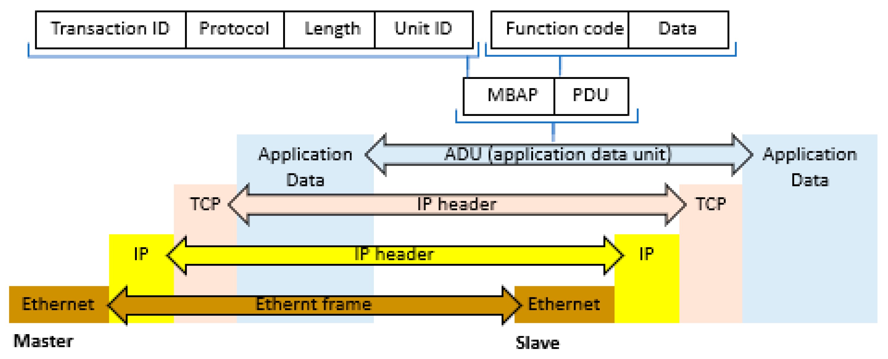
Figure 1 [
23] presents the communication between slave and master devices connected in a Modbus TCP/IP network. The data unit (ADU) consists of the protocol header (MBAP) and the Modbus protocol frame data (function code and data/parameters; PDU). The data unit is built by the device initiating the transaction, in the case of the Modbus protocol this is the master. The function codes define the type of action to be performed by slaves. The Modbus commands and user data are encapsulated in the data container of a TCP/IP packet without any modification. However, the Modbus checksum field is not used, as the protocol relies on the standard Ethernet TCP/IP link layer checksum to guarantee data integrity. Furthermore, the Modbus TCP/IP frame utilizes the address field to carry the unit identifier and becomes part of the Modbus Application Protocol (MBAP) header.
Selected bits from the frame are used to distinguish messages for the purpose of identification. The meaning of the bytes in the frame is presented in the list below:
Transaction identifier (2 bytes): set by the master to correctly associate responses to its subsequent queries. This value is determined and placed in the query frame by the master, and then copied and placed in the response frame by the slave;
Protocol identifier (2 bytes): always set to 00, which indicates the Modbus protocol;
Length (2 bytes): set by the master. It specifies the number of remaining bytes in the message (starting from the unit identifier field);
Unit identifier (1 byte): set to master—the value repeated by the slave device to uniquely identify the slave device;
Function code (1 byte): defines what kind of action the addressed slave device should perform; the Modbus standard defines only 19 of the 127 possible function codes;
Data bytes (n bytes): data as response or commands.
When a task is performed, the slave sends back a response packet containing the request function code and the proper data corresponding to the performed function. In the case of failure, the function code and error code are returned.
In request and response Modbus cyclic communication, the values of some fields in the frame are fixed and can be used as the distinguisher to identify the communication channel of two devices. In this research, the following fields were used as the distinguisher: master and slave IP, protocol identifier, unit identifier, and function code. Additionally, register addresses are considered in the distinguisher for read and write functions.
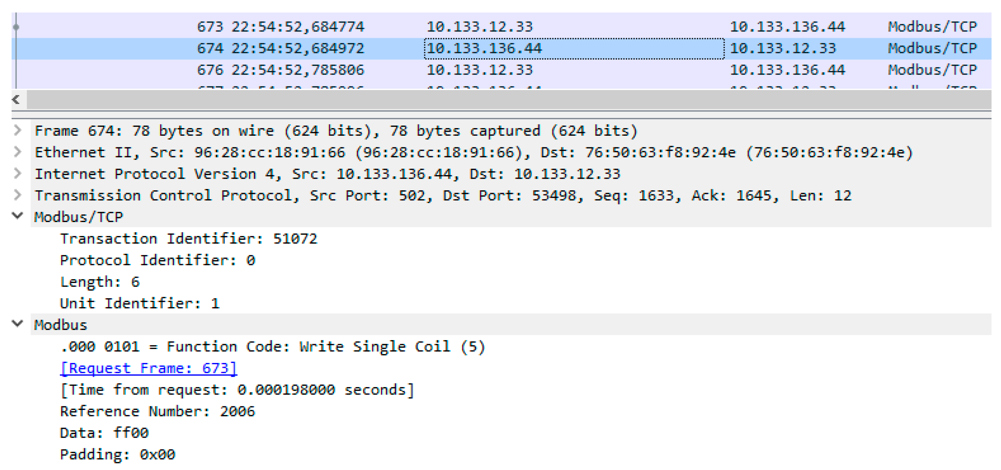
The communication example (screen from wireshark) is presented in
Figure 2.
Communication in OT protocols depends on the nature of cyclic information exchange between subsystems. For multiple devices, communication can occur at different frequencies and can be disrupted by single or multiple non-cyclic events. Two models are proposed to describe this type of information exchange, which are described in the next section.
4. Communication Coding Models
The study of message sequences requires the use of description in the form of a model. The comparison of the current message sequence with the model record allows detection of anomalies that may indicate that an attack was carried out. This paper uses a model in the form of a graph built as a graphical form of a deterministic finite automaton and a model in the form of cycles.
4.1. Deterministic Finite Automaton
Deterministic finite automata (DFA) are finite state automata [
24]. A DFA can be represented as a machine with a finite number of states, a table of transitions between states, or a state diagram.
After reading each word, the automaton changes its state to a state that is the value of a function of one symbol read and the current state. If, after reading the entire word, the machine is in any of the states marked as accepting (final), the word belongs to the regular language it is built to recognize.
An automaton is deterministic if it can only move to one state after reading a given symbol. An automaton is finite if there are a finite number of possible states that can be reached. A finite automaton is only called deterministic (DFA) if it satisfies both conditions.
A DFA is described by five components [
25], denoted by a set of five symbols called 5-tuples (Q, ∑, δ, q
0, F).
The form of deterministic finite automata allows network traffic to be described as a graph; the structure of that model is shown in
Section 4.2.
4.2. Graphic Form of the Automaton
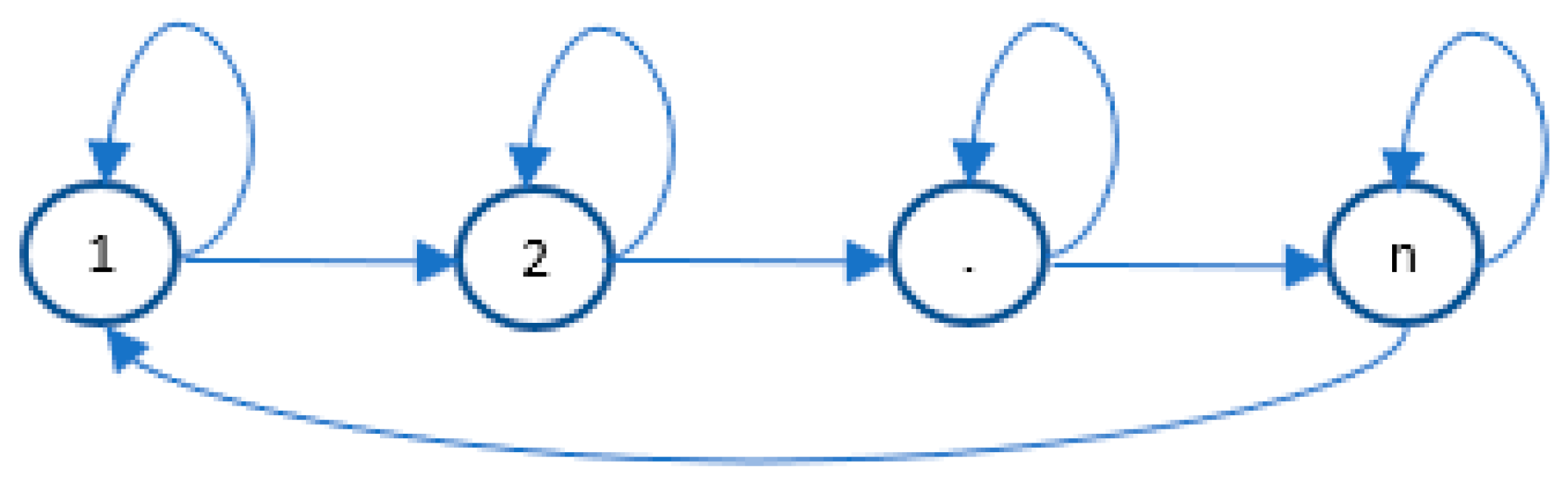
DFA can be used as a model of cyclic device communication and described by a graph. In the case of string analysis, the task of the automaton is to determine whether a word belongs to an established language. In the case of modbus communication analysis, the task is analogous. The goal is to check whether the sequence of commands sent between devices is correct, i.e., whether the sequence of commands belongs to a learned pattern.
Command codes will be used as the alphabet ∑. The states of the Q automaton represent the state in the modbus communication. If the set of command codes is finite, then the set of states is also finite. The command code message δ is interpreted as a transition function.
One difference from conventional DFA is that there is no requirement for acceptance states because an infinite repeating stream (communication between devices) is continuously monitored by the intrusion detection system. Any anomaly observed as a deviation from the reference model is recorded as an attack. There is also a difference when determining the initial state, which is defined as the state corresponding to the first query recognized in the periodic network traffic related to Modbus protocols. Only Modbus frames are monitored. A model coding the query sequence 1…1, 2…2, …, n…n, 1…1, … is presented in
Figure 3.
4.3. Cycle Construction Algorithm
An alternative model to the graph can be used to model coding communication cycles. The problem of finding cycles is widely described in the literature [
26]. These materials were the basis for developing our own approach, which is better adapted to the problem studied and nature of transfer data where cyclicality can be disrupted.
The cycle extraction algorithm is a four-step iterative algorithm, the next steps of which are presented below.
Initial conditions:
Set initial iteration number f = 1, set initial cycle number k = 1;
Step 1, iteration f, cycle k:
Search for the next most frequent query (distinguisher) mf;
Step 2, iteration f, cycle k:
Determining:
- ○
Sf—the set of common queries recorded between consecutive moments in which the query mf was recorded;
- ○
Vf—the occurrence vector specifying the number of query occurrences.
Step 3, iteration f:
If possible, determine the cycle set Ck = {mf, Sf} and the vector of number of occurrences Nk = [1, Vf], and remove the cycle queries from the data. Set k = k + 1.
If there is more than one type of query and there are still queries that were not considered, go to step 1 and set f = f + 1.
Step 4, end of algorithm:
The queries that are not classified according to the cycles are treated as exceptions.
The algorithm ends iterations when all queries have been grouped into cycles. The queries that remain will be classified as a set of independent exceptions E, which are interpreted as queries that can occur at any time independently of other queries.
Building the list of queries related to cycles can be done within a pair of devices (for each pair independently) or globally without distinguishing between devices, which may make sense when there is a strict regularity of the work of devices—e.g., communication is synchronized by a common system time.
The operation of the algorithm has been illustrated using an example, assuming a certain data transfer (presented in
Figure 4), and assuming that the data are sent with a different frequency in different cycles. Each number corresponds to a unique request (data sent from the sender or the receiver), where uniqueness is determined by specific features, such as function code, selected arguments, layout and values of status fields, and device identifiers.
Example: Cycles-finding algorithm.
Initial conditions:
f = 1, k = 1.
Step 1, iteration f = 1, cycle k = 1: Search for the next most frequent query (distinguisher) m1—in the presented example for f = 1 and k = 1, this is “2”.
Step 2, iteration f = 1, cycle k = 1: Determining:
- ○
S1—the set of common queries recorded between consecutive moments in which the query m1 was recorded—in the example shown, the following sets of queries occur sequentially between successive “2” queries: empty set {} between 1st and 2nd “2” query, {3,4,5,7,9,1} set of queries between 2nd and 3rd “2” query, etc.
The common S1 is an empty set. In other words, it is not possible to determine the common set of queries.
- ○
V1—the occurrence vector specifying the number of query occurrences—in this example for f = 1 and k = 1, this is empty.
Step 3, iteration f = 1, cycle k = 1: Since S1 is empty, it is not possible to determine the cycle set C1 = {m1, S1} and the vector of number of occurrences N1 = [1, V1], and remove the cycle set queries from the data.
Set f = f + 1.
Step 1, iteration f = 2, cycle k = 1: Search for the next most frequent query (distinguisher) m2—in the presented example for f = 2 and k = 1, this is “9”.
Step 2, iteration f = 2, cycle k = 1: Determining:
- ○
S2—the set of common queries recorded between consecutive moments in which the query m2 was recorded—in the example shown, the following sets of queries occur sequentially between successive “9” queries: {3,4,5,7} between 1st and 2nd “9” query, {1,2,2,3} set of queries between 2nd and 3rd “9” query, {4,1,5,2,2} set of queries between 3rd and 4th “9” query etc.
The common S2 is an empty set, in other words it is not possible to determine the common set of queries.
- ○
V2—the occurrence vector specifying the number of query occurrences—in this example for f = 2 and k = 1, this is empty.
Step 3, iteration f = 2, cycle k = 1: Since S2 is empty, it is not possible to determine the cycle set C1 = {m2, S2} and the vector of number of occurrences N1 = [1, V2], and remove the cycle set queries from the data.
Set f = f + 1.
Step 1, iteration f = 3, cycle k = 1: Search for the next most frequent query (distinguisher) m3—in the presented example for f = 3 and k = 1, this is “3”.
Step 2, iteration f = 3, cycle k = 1: Determining:
- ○
S3—the set of common queries recorded between consecutive moments in which the query m3 was recorded—in the example shown, the following sets of queries occur sequentially between successive “3” queries: {5,7,9,1,2,2} between 1st and 2nd “3” query, {9,4,1,5,2,2,9} set of queries between 2nd and 3rd “3” query, {9,1,2,7,2} set of queries between 3rd and 4th “3” and (4,5,9,1,2,2} set of queries between 4th and 5th “3” query.
The common S3 is {1,2,2,9}.
- ○
V3—the occurrence vector specifying the number of query occurrences—in this example for f = 3 and k = 1, this is [1,2,1 or 2]—query “9” can occur once or twice during the cycle.
Step 3, iteration f = 3, cycle k = 1: C1 = {m3, S3} = {3,1,2,9} and the vector of number of occurrences N1 = [1, V3] = [1,1,2,1 or 2], k = k + 1.
Set f = f + 1.
Step 1, iteration f = 4, cycle k = 2: Search for the next most frequent query (distinguisher) m4—in the presented example for f = 4 and k = 2, this is “4”.
Step 2, iteration f = 4, cycle k = 2: Determining:
- ○
S4—the set of common queries recorded between consecutive moments in which the query m4 was recorded—in the example shown, the following sets of queries occur sequentially between successive “4” queries: {5,7} between 1st and 2nd “4” query, {5,7} set of queries between 2nd and 3rd “4” query, {5} set of queries between 3rd and 4th “4” query.
The common S3 is {5}.
- ○
V4—the occurrence vector specifying the number of query occurrences—in this example for f = 4 and k = 2, this is V4 = [1].
Step 3, iteration f = 4, cycle k = 2: C2 = {m2, S4} = {4,5} and the vector of number of occurrences N1 = [1, V4] = [1,1], k = k + 1.
The list of queries only contains query “7”.
Step 4, end of algorithm.
Applying the algorithm to the data in the example leads to the following solution: C1 = {3,1,2,9}, N1 = [1,1,2,1 or 2], C2 = {4,5}, N2 = [1,1], E = {7}
5. Anomaly Detection Algorithm
5.1. Graph
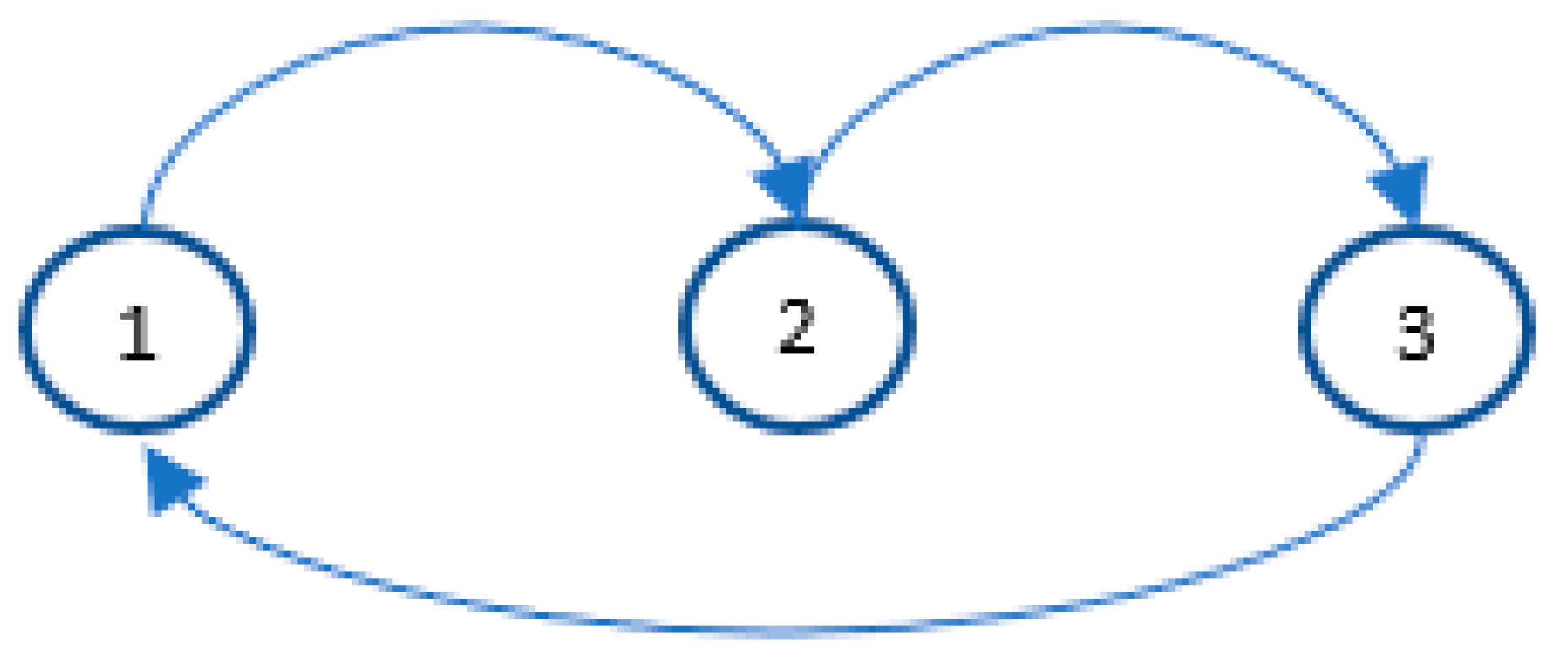
The anomaly detection algorithm is based on graph construction. The algorithm consists of checking in real time whether queries are present in the graph and whether they arrive according to possible cycles present in the graph. An explanation is provided by the example, so let’s consider the graph in
Figure 5.
In the presented case, anomaly detection will occur if the queries arrive in a sequence other than “1”, “2”, “3”. This means that a different order, e.g., “1”, “3”, “2”, or a query arriving more than once, e.g., “1”, “2”, “2”, “3”, will be classified as an anomaly or a potential attack.
The graph-based algorithm is easier to implement and faster to run but seems to be less restrictive when dealing with multiple channels. The property of the method is a subject of the tests described in the next section.
The aim of the paper is to show algorithmic mechanisms. Therefore, in order to simplify the presentation, “repeat” messages were not included in the research.
5.2. Cycle List
The algorithm consists of continuously checking whether incoming messages mk arrive according to the description determined by cycles Cx and occurrence vectors Nx. If a query does not come or comes more times than defined, then such an event is treated as an anomaly or a potential attack.
The verification algorithm is run in a mode analogous to the algorithm responsible for building cycles, that is, in a mode that monitors each pair of devices independently or globally without distinguishing between devices.
5.3. Time Domain Extension
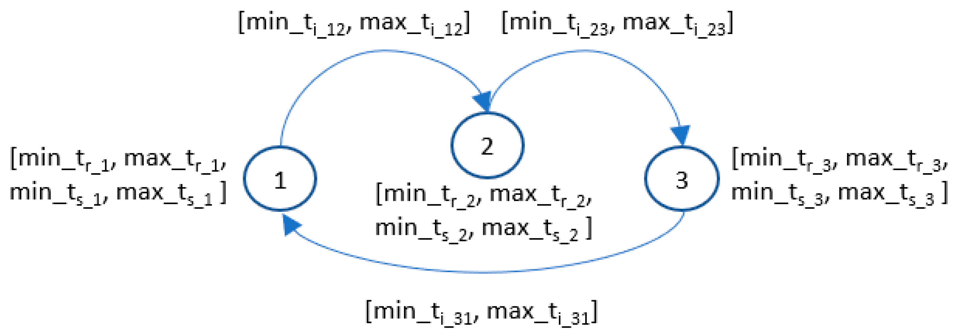
Both algorithms described in the previous sections can be extended to measure the time between messages. Extending the measurement of time between exchanged messages introduces stochastic elements into the algorithm. The result is an algorithm that combines a deterministic approach based on modeling consecutive messages with a model that allows random deviations of regularity. It is proposed to measure the times between:
incoming x and y requests as ti_xy
request and response for x request as tr_x
the same x request as ts_x
The extended version algorithm checks if the current measurements range between minimum and maximum values. The minimum and maximum values are collected while the algorithm learns regular plant operation. The additional parameters are:
Four parameters for each node: max_tr_x, min_tr_x, max_ts_x and min_ts_x,
Two parameters for each pair of connected x and y nodes: max_ti_xy and min_ti_xy.
The extended graph is presented in
Figure 6.
The algorithm continuously monitors the times at any k moment (t
r_x_k, t
s_x_k, t
i_xy_k) and checks whether the minimum and maximum values have been exceeded. Exceeding the values can indicate that an anomaly has occurred, which may be the result of an attack and should be identified by the algorithm. The behavior of the algorithm for each x node and for each pair of connected x and y nodes can be described by the Equations (1)–(3). If any variable is equal to TRUE, the algorithm reports the detection of the anomaly and the suspected attack.
In the case of a cycle list, the extension is coded as additional vectors: min_Ti_xy, max_Ti_xy, min_Tr_x, max_Tr_x, min_Ts_x, and max_Ts_x defined for each cycle, where the meaning of the vectors is analogical to the meaning of the variables used in the graph. Based on the results from the example for the first cycle: C1 = {3,1,2,9}, N1 = [1,1,2,1 or 2], min_Tr_x, max_Tr_x, min_ Ts_x, and max_Ts_x are 4th element vectors (due to the number of elements in C1), and min_Ti_xy and max_Ti_xy are 6th element vectors (due to N1 values). They define the min and max value of the time between queries and the minimum and maximum value of the response time.
6. Results
6.1. Research Environment
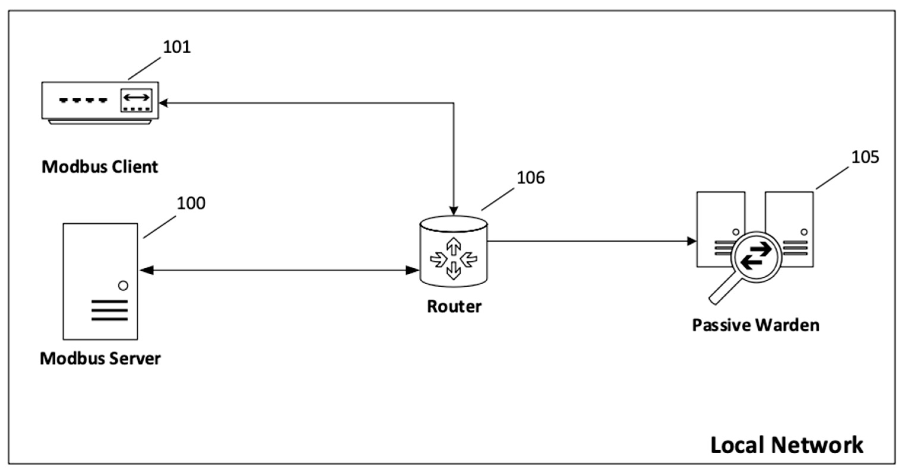
We conducted the experiment using two architectures for data collection and further testing. The first experiment (presented in
Figure 7) was conducted in an environment consisting of two endpoints: server (100) and client (101), which have established a channel and exchange Modbus protocol messages, among other network traffic. Both devices are on a local area network where all network traffic passes through a core router. The core router sends a copy of all traffic to the passive warden. Only messages sent over the Modbus protocol are analyzed.
All the algorithms described in this paper have been implemented and run as part of a passive guard system. The passive guard is implemented in C/C++ as part of a larger commercial IDS (intrusion detection system). Proven mechanisms for communication, frame collection and parsing, and timing were used. The functions of the new methods were previously prototyped in Python, and a 10-gigabit Ethernet connection was used.
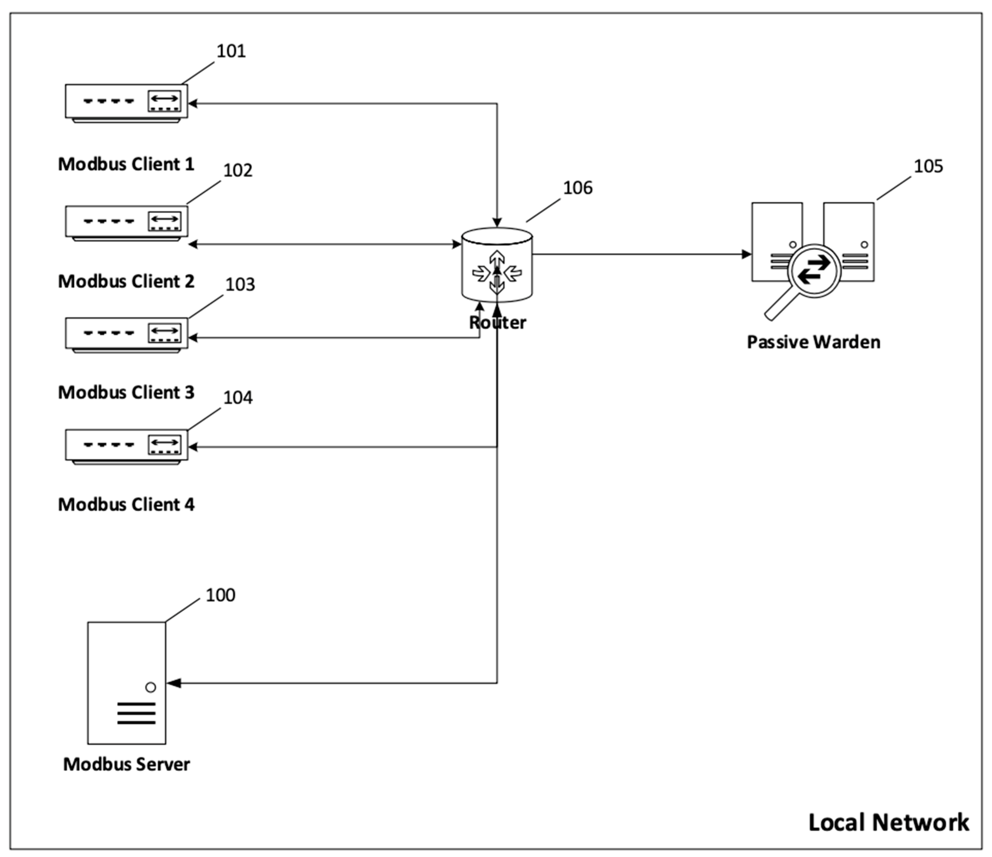
The second and third experiments were conducted in an environment consisting of one server (100) and four clients (101–104) presented in
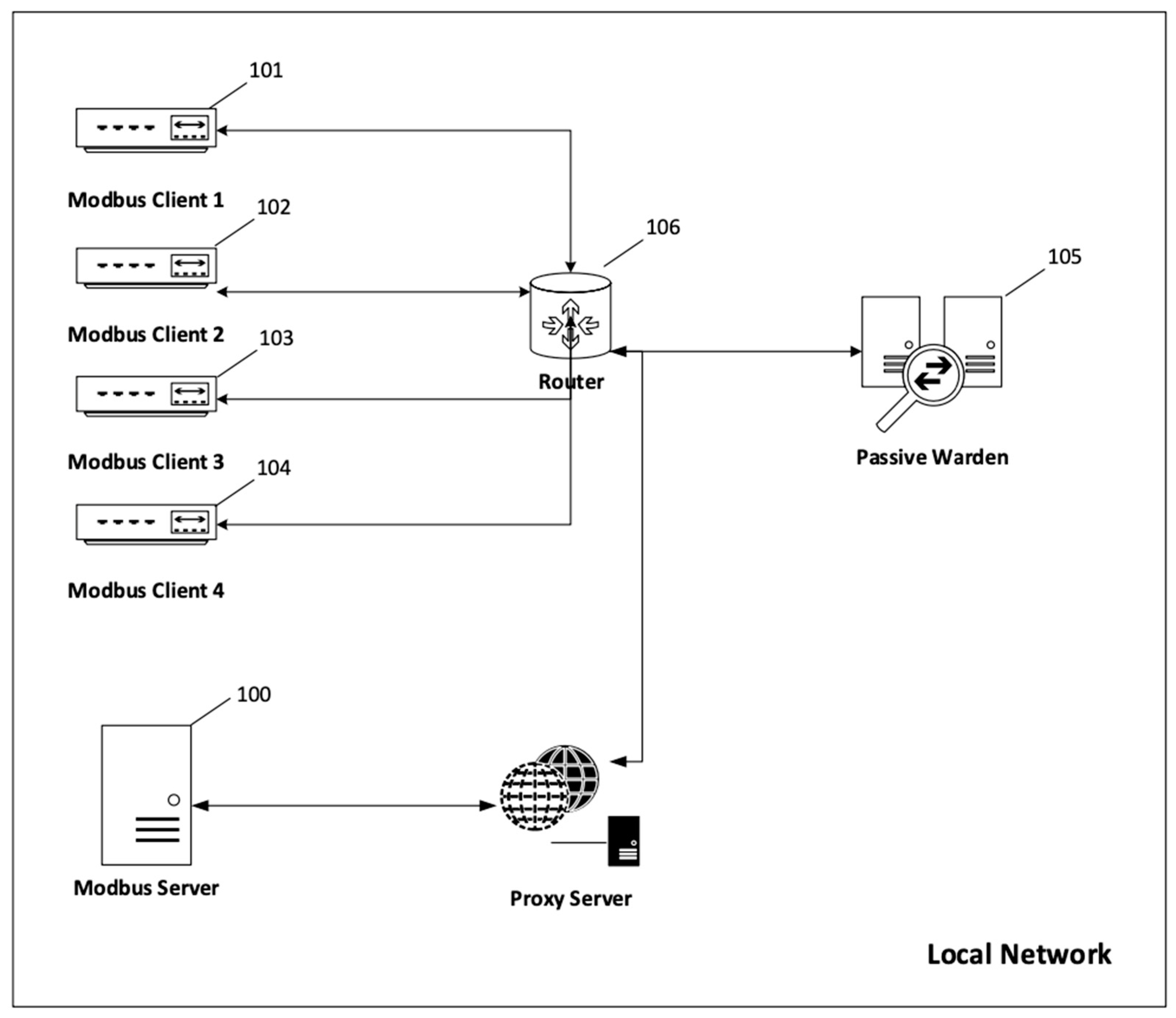
Figure 8. Each client has established a channel and exchanges Modbus protocol messages, among other network traffic. All devices are on a local area network where all network traffic passes through a core router. The core router sends a copy of all traffic to the passive warden. Only messages sent over the Modbus protocol are analyzed. In the third experiment, the structure is extended around the proxy device (presented in
Figure 9) to simulate an attack utilizing the C&C steganographic channel.
In the third experiment, the structure is extended around the proxy device to simulate an attack utilizing the C&C steganographic channel.
6.2. Experiment Methodology
In the first phase of the experiment, there was no interference in communication between the client and server, exemplary traffic was conducted (1000 min for example 1 and 2 and 100 min for example 3), which allowed a reference communication model to be built. Simulated attacks were tested in the second phase of the test. Tests were repeated four times for each case. The details of the transmitted commands along with the attack scenarios are discussed in the examples.
6.3. The Results for Example 1
First case: master–slave (one server—one client) communication. The client reads ten input registers from the server (starting from address 30,001) and writes one single register to the server (using address 40,001). Communication takes place in a task that runs every 100 milliseconds.
Five types of attacks were tested:
Attack 1: Reads data from a random register at a random time
Attack 2: Writes data to a random register at a random time
Attack 3: Reads data from the register used at a random time
Attack 4: Writes data to the register used at a random time
Attack 5: Uses a command that did not occur before
An attack was considered a single command occurring at a random time during a one-minute simulation. During a single one-minute simulation, each type of attack was executed only once at a random moment. A total of 5000 attacks were executed during 1000 one-minute simulations. The tests were repeated four times, with the results for each case shown in
Table 1 in columns Test 1 to Test 4, respectively.
6.3.1. Graph
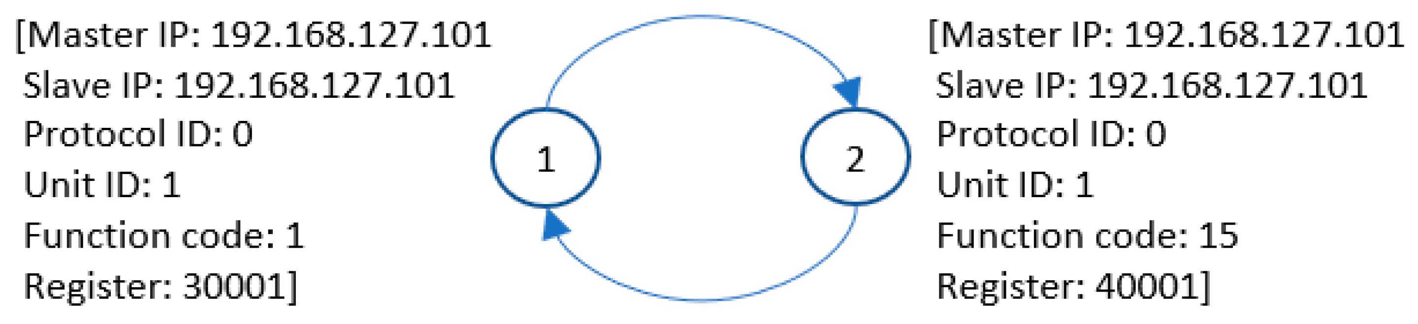
The structure of the graph that models the traffic for the first example is very simple (
Figure 10) and is presented only to explain the algorithm properties. In this example, the graph only has two nodes, which are associated with the read and write commands. Node “1” codes the following message information (used as a distinguisher): master and slave IP, protocol identifier, unit identifier, function code, register addresses. Similarly, for calling the node “2”, the difference lies in the function code and registers.
It is obvious the model detected all 5-type attacks because code functions other than 1 and 15 do not fit the traffic model. Similarly, the model detected all 1- and 2-type attacks because the probability of attacks 1 and 2 executing in a sequence consistent with the model is very low. If there are 9999 registers that can be read (in the range 30,001 to 39,999) and 9999 registers that can be written (in the range 40,001 to 49,999), then the probabilities can be described by (4) and (5).
Additionally, the probability of the correct sequence of attacks and the time between them must be considered. The probabilities can be described by (6) and (7).
Considering these equations, the final probability of not detecting attacks 1 and 2 in one try is about 8.3 × 10⁻¹². That probability is very low, and it explains why all 2- and 3-type attacks were detected.
The model presented flawlessly detected almost all anomalies. However, when the sequence of anomalous messages matched the sequence of correct communication messages, such an anomaly was not detected. It happened a few times for 3- and 4-type attacks. In attacks 3 and 4, the registers are set to the correct values (30,001 and 40,001) and the probability that attacks 3 and 4 will be executed in the model order is described only by (6) and (7) and for one try equals 1/1200. Example 1 was performed four times. The number of simulations when the anomaly (attacks 3 and 4) was not detected during 1000 one-minute simulations is presented in
Table 1.
Based on the results obtained, the efficiency was calculated using two algorithms defined by Equations (8) and (9)
where N
s defines the number of simulations (1000 for one test) and N
nds defines the number of simulations when the attack was not detected and
where N
m defines the number of messages. For a one-minute simulation, there are 600 read commands, 600 write commands, and five attack commands, totaling 1,205,000 messages during 1000 simulations. N
ndm defines the number of undetected attack messages. The efficiency results for Efficiency
1 and Efficiency
2 are presented in
Table 2 and
Table 3.
The very good results are due to the very simple communication used in this example. For more complex communication, the results are much worse, as shown in Example 2 in
Section 6.4.1 and
Section 6.4.2. An alternative method that is more robust is shown in Example 2 in
Section 6.4.3.
6.3.2. List of Cycles
Based on the results from the first experiment, one cycle was defined: C1 = {1,2}, N1 = [1,1]. For this simple example, the cyclic model is identical to the graph model. The effectiveness calculated using the two methods (8) and (9) of the cyclic list was identical to that of the graph. Moreover, there was a problem with detection when the sequence of anomalous messages matched the sequence of correct communication messages.
6.3.3. Time Domain Extension
The time domain extension in the presented example improved the result and efficiency increased to 100% for both methods: cyclic list and graph. An attempted attack using a sequence of messages from normal communication is immediately apparent at times ti and ts.
6.4. The Results for Example 2
Second case: master–slave (one server—four clients) communication. There are four clients running:
Client 1: reads ten input registers from the server (starting from address 30,001). The process is executed in a task that runs every 30 ms.
Client 2: reads eight input registers from the server (starting from address 30,011). The process is executed in a task that runs every 40 ms.
Client 3: writes one single register to the server (using address 40,021). The process is executed in a task that runs every 100 ms.
Client 4: writes one single register to the server (using address 40,041). The process is executed in a task that runs every 150 ms.
Five types of attacks were tested:
Attack 1: Reads data from a random register at a random time
Attack 2: Writes data to a random register at a random time
Attack 3: Reads data from the register used at a random time
Attack 4: Writes data to the register used at a random time
Attack 5: Uses a command that did not occur before
An attack was considered a single command occurring at a random time during a one-minute simulation. During a single one-minute simulation, each type of attack was executed only once at a random moment. A total of 5000 attacks were executed during 1000 one-minute simulations. The tests were repeated four times. The results for each case are shown in
Table 2 in the columns Test 1 to Test 4, respectively.
6.4.1. Graph
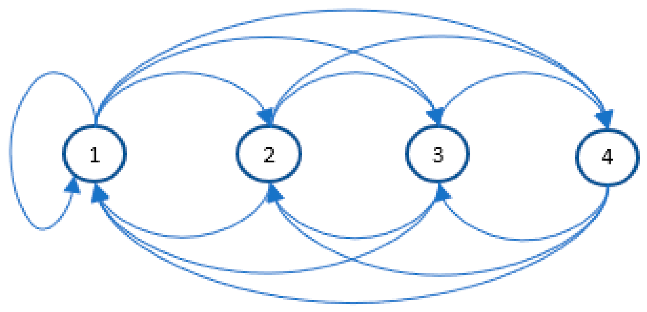
The structure of the graph that models the traffic for this example is more complex (
Figure 11). The graph has four nodes, which are associated with the read and write commands. Due to the different periods of customer communication, the resulting graph has the form of a directed completed graph. Each node, like the previous example, codes the following message information (used as a distinguisher): Master and slave IP, protocol identifier, unit identifier, function code, register addresses.
If, during the attack, functions or registers not present in the model traffic are used, the model presented detects the attack with 100% efficiency, analogically to example 1. If the same functions and registers are used, the model detected only a small percentage of attacks. Example 2 was also performed four times. The number of cases when attacks 3 or 4 were not detected (N
t) during 1000 (N
s) one-minute simulations is presented in
Table 4.
Efficiency is counted using Equations (8) and (9) in the same manner as in Example 1. The number of simulations is identical (N
s = 1000); the difference is the number of messages caused by the higher number of clients and different sampling time. For the one-minute simulation, there were 2000 read commands generated by client 1, 1500 read commands generated by client 2, 600 write commands generated by client 3, 400 write commands generated by client 4, and five attack commands, totaling 4,505,000 messages during 1000 simulations. The efficiency results for Efficiency
1 and Efficiency
2 are presented in
Table 5 and
Table 6.
The example presented shows that for more complex network traffic, the efficiency of the graph-based model can be low. The efficiency calculation methods presented in this paper show the results can vary significantly. The first method based on Equation (8) is a better presentation of the results.
Improved performance can be achieved by building independent graphs for each client-server channel. However, that approach is limited because more than one link can run in client–server communication. A much more effective approach is to use the time domain extension. That approach is discussed in
Section 6.4.3.
6.4.2. Cycle List Model
In this case, two cycles are defined using the algorithm presented in this paper: C
1 = {2,1}, N
1 = [1,2 or 3], C
2 = {4,3}, N
2 = [1,1 or 2]. If functions or registers not present in the model traffic are used, the model presented (like graph) detects the attack with 100% efficiency. If the same functions and registers are used, the model did not detect all attacks. Example 2 for the cycle list was also performed four times. The number of cases when attacks 3 or 4 were not detected during 1000 one-minute simulations is presented in
Table 7.
Efficiency is counted in the same way using Equations (8) and (9). The efficiency results for Efficiency
1 and Efficiency
2 are presented in
Table 8 and
Table 9.
Compared with the graph, the cyclic list shows significantly higher efficiency. The cyclic list remembers sequences of commands, while errors in detection occur only when a query is generated as an attack, which may occur a different number of times. To improve efficiency, a time domain extension can be used. That approach is discussed in
Section 6.4.3.
6.4.3. Time Domain Extension
The graph in the extended form does not correctly show time ti_xy. The problem is the result of overlapping sequences, which cause the time between successive queries to be inconsistent. However, there are no problems with times tr_x and ts_x. Each attempted attack was detected by a deviation in time ts_x. Extended in a time domain, the graph detected the attack with 100% efficiency.
The list of cycles in extended form also achieved a 100% success rate. As in the graph case, all attempted attacks were detected by a deviation in time Ts_x.
6.5. The Results for Example 3
Third case: master–slave (one server—four clients) communication with proxy in the middle. In this case, the same master-slave structure was used. There are four clients running:
Client 1: Reads ten input registers from the server (starting from address 30,001). The process is executed in a task that runs every 30 ms.
Client 2: Reads eight input registers from the server (starting from address 30,011). The process is executed in a task that runs every 40 ms.
Client 3: Writes one single register to the server (using address 40,021). The process is executed in a task that runs every 100 ms.
Client 4: Writes one single register to the server (using address 40,041). The process is executed in a task that runs every 150 ms.
The difference lies in the hardware environment extended around the new element to simulate a command-and-control phase of attack utilizing a covert (steganographic) channel.
One test lasted two minutes. Over 100 tests were performed during the experiment, varying the network load (generating additional traffic) within a range of ±40%, which is reasonable for stable industrial networks. During one test, 9000 queries were generated (4000 from client 1 running a 30 ms task, 3000 from client 2 running a 40 ms task, 1200 from client 3 running a 100 ms task, and 800 from client 4 running a 150 ms task). About 900,000 samples were collected, half of them for regular system operation.
In the case studied, the same communication scheme (same messages) was used, and the same models were also used for detection. The attack consisted of changing the values of transmitted registers, while the values of addresses were not changed.
6.5.1. Graph
Covert channel attacks affect the graph model in cases where a message sequence is changed. In the other cases, the graph model remains unchanged by steganographic channels. If the sequence of queries is maintained, the model in the form of a graph will not be able to detect an anomaly, i.e., such an attack will not be recognized. It is worth emphasizing that the probability of carrying out an attack in which only the parameter values have been changed, and the function codes remain the same, is relatively low, but nevertheless it is not zero. Protection against the aforementioned risk is provided by use of the time dependency measurement, i.e., the use of a method based on a graph extended in the time domain.
6.5.2. List of Cycles
As with the graph model, the list-of-cycles model does not detect covert channel attacks at all if the message sequence is not changed. The method based on cyclic lists, like the graph, is sensitive only to examining the sequence of incoming queries. In the case of a cleverly crafted attack, this method, just like the graph-based method, may turn out to be ineffective. As in the previous case, the use of the time dependency measurement, i.e., the use of the extended method in the time domain, solves the above-mentioned problem.
6.5.3. Time Domain Extension
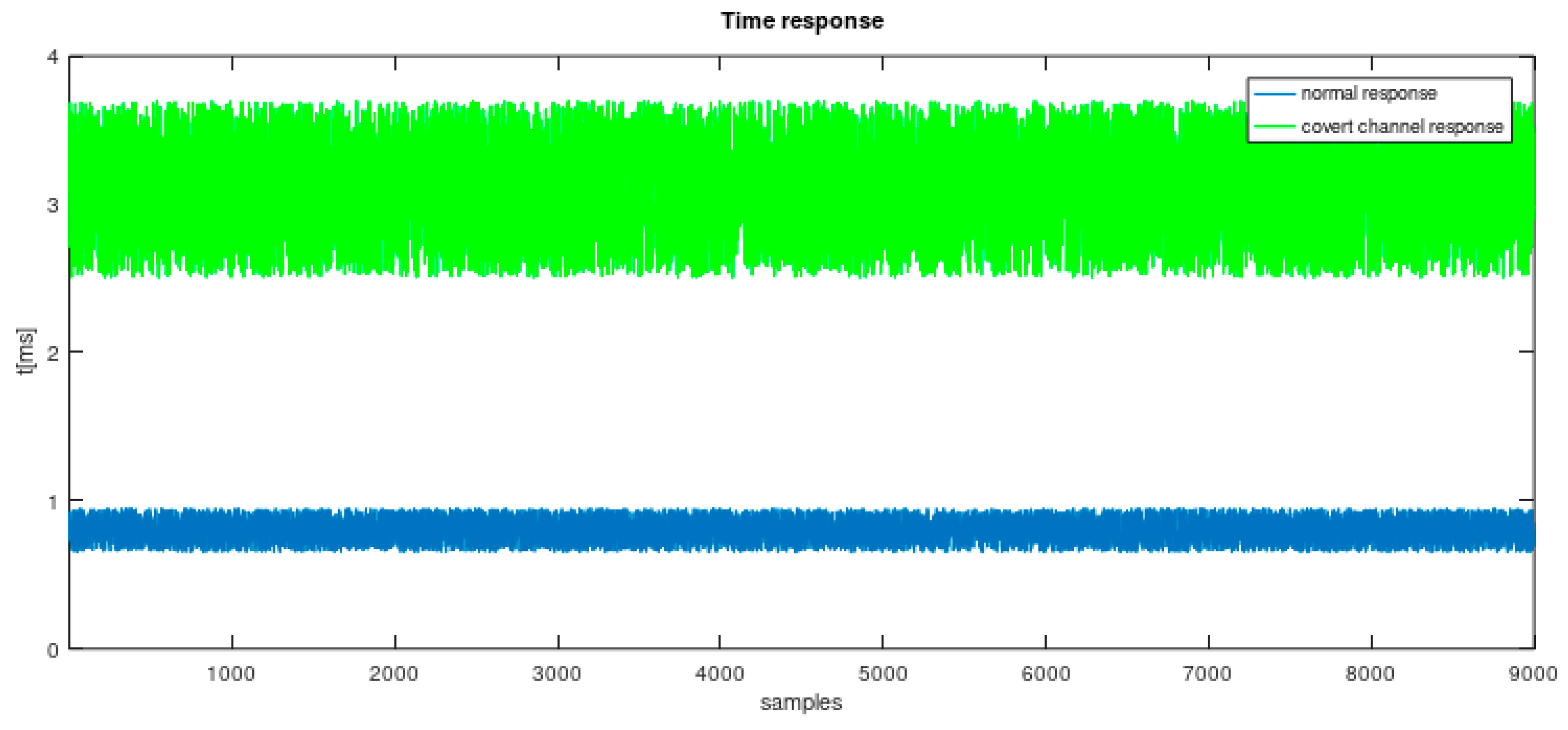
Covert channel attacks can be detected based on response time analysis. Message routing and processing during the attack adds constant delay. Both cyclic lists and the graph extended by timing measurements allow for covert channel attack detection. The time of response for the classic structure and the structure with proxy device is presented in
Figure 12.
The experiment consisted of measuring the ∆t parameter during normal system operation and during a simulated man-in-the-middle attack. The experiments showed that introducing an additional communication intermediary device between the client and the server substantially increases the time between sending a request and receiving a response. No significant effect of network load on response time was observed. Response. time analysis enables anomalies and potential attacks to be easily identified.
7. Conclusions
The anomaly detection algorithm presented in the paper is easy to implement and quick to operate. Two approaches were proposed: the first based on a graph inspired by a finite state automaton, and the other is a proprietary algorithm based on cyclic lists. Both solutions have been shown to be very effective and can be successfully used in sensing probes and systems based on modern high-speed industrial networks. For single-channel communication, both approaches produce the same results. Most attack scenarios presented are detected, including command-and-control covert channels, unless the sequence of attack commands is chosen so that it coincides with the sequence observed during normal traffic.
For multi-channel communication or multiple links running between two systems, the cyclic list-based algorithm is much more effective. Again, if the attack is constructed such that the attack sequence is identical to the command sequence during normal traffic, such an attack will not be recognized. The introduction of time-to-response and time-between-messages measurements allowed detection of all attacks carried out, and even the attack sequence is identical to the command sequence during normal traffic.
These extensions in the time domain introduce stochastic elements into the algorithm. The result is a novel algorithm combining finite automaton determinism modeling consecutive admissible messages with a time-domain model allowing for random deviations of regularity. The algorithm features high efficiency and easy scalability. The algorithm aims to detect attacks that operate on many kill chain phases. Typically, the first phase is usually a network reconnaissance when messages inconsistent with the determinism of the sequence of incoming messages appear. Subsequent phases usually comprise proper attack techniques that operate directly on registers of process variables. A direct attack often involves sending additional messages that do not change the sequence of messages but instead change the time regularity. The study was conducted for several test scenarios, including a steganographic C&C channel generated using the Modbus TCP/IP protocol.
For command-and-control covert channel detection, the best approach is cycle recognition based on response time. The cyclic list and graph approach did not provide optimistic detection results. In contrast to other types of attacks, steganographic channel detection usually requires a specialized forensics analysis. The value added by the algorithm is the pre-selection of anomalous traffic. Outliers in a cyclic communication channel can be a strong indicator of a network steganographic channel.
The presented techniques cover the white-list technique fully, specifying which applications and which commands are allowed. Additionally, they specify the permitted sequences and times, which makes them much more effective.
Industrial communication is characterized by high regularity, while cyclicity creates another dimension to studying deviations. These features are used in this paper, in which the authors have presented a method for detecting anomalies in cyclic communication using the Modbus protocol. In addition to the above features, the proposed method has another advantage: The automatic identification of the model in the learning phase makes the algorithm easy to implement and deploy. Moreover, the user does not need to determine probability or other parameters that are difficult to estimate in real industrial traffic.
However, it would be interesting to compare the proposed method with other methods based on nondeterministic methods (e.g., nondeterministic finite state automata, or NFSA) or stochastic and probabilistic models such as Markov processes [
27]. Research on the frequency domain or using other model structures like the attack tree [
28] are also possible. These directions will be explored in further research.
Author Contributions
M.S. contributed to theoretical formulation, design methodology, dataset development, experiment design and implementation, results interpretation, original draft preparation, and revision. The other authors (S.P., J.P. and K.S.) contributed to project supervision, theoretical formulation, result interpretation, and revision of the initial draft. All authors have read and agreed to the published version of the manuscript.
Funding
This scientific research work was co-financed by the European Union under the project name “The system for securing industrial networks.” The amount financed by the European Union totals €1,072,193.52. The investment outlay value for the entire project totals €1,415,884.27. The subsidy was allocated from the European Regional Development Fund, Operational Program “Smart Growth,” sub-measure 1.1.1 “Industrial research and development work implemented by enterprises” (grant number: POIR.01.01.01-00-0125/19).
Conflicts of Interest
The authors declare no conflict of interest.
References
- Wang, D. Building value in a world of technological change: Data analytics and Industry 4.0. IEEE Eng. Manag. Rev. 2018, 46, 32–33. [Google Scholar] [CrossRef]
- Ancarani, A.; Di Mauro, C. Reshoring and Industry 4.0: How often do they go together? IEEE Eng. Manag. Rev. 2018, 46, 87–96. [Google Scholar] [CrossRef]
- Sony, M.; Naik, S.S. Ten lessons for managers while implementing Industry 4.0. IEEE Eng. Manag. Rev. 2019, 47, 45–52. [Google Scholar] [CrossRef]
- Malik, A.K.; Emmanuel, N.; Zafar, S.; Khattak, H.A.; Raza, B.; Khan, S.; Al-Bayatti, A.H.; Alassafi, M.O.; Alfakeeh, A.S.; Alqarni, M.A. From Conventional to State-of-the-Art IoT Access Control Models. Electronics 2020, 9, 1693. [Google Scholar] [CrossRef]
- Zafar, F.; Khan, A.; Anjum, A.; Maple, C.; Shah, M.A. Location Proof Systems for Smart Internet of Things: Requirements, Taxonomy, and Comparative Analysis. Electronics 2020, 9, 1776. [Google Scholar] [CrossRef]
- Knapp, E.D.; Langill, J.T. Industrial Network Security Securing Critical Infrastructure Networks for Smart Grid, SCADA, and Other Industrial Control Systems; Elsevier: Amsterdam, The Netherlands, 2015. [Google Scholar]
- NIST. “800-82,” Guide to Industrial Control Systems (ICS) Security, Rev. 2; National Institute of Standards and Technology: Gaithersburg, MD, USA, 2015.
- ISA-99.00.01; Security for Industrial Automation and Control Systems—Part 1: Terminology, Concepts and Models American National Standard. International Society of Automation: Pittsburgh, PA, USA, 2007.
- Neubert, T.; Claus Vielhauer, C. Kill Chain Attack Modelling for Hidden Channel Attack Scenarios in Industrial Control Systems. In Proceedings of the 21st IFAC World Congress (Virtual), Berlin, Germany, 12–17 July 2020; Volume 53, pp. 11074–11080. [Google Scholar]
- Slammer Worm and David-Besse Nuclear Plant. 2015. Available online: https://large.stanford.edu/courses/2015/ph241/holloway2/ (accessed on 20 October 2021).
- Nourian, A.; Madnick, S. A systems theoretic approach to the security threats in cyber physical systems applied to stuxnet. IEEE Trans. Dependable Secur. Comput. 2015, 15, 2–13. [Google Scholar] [CrossRef] [Green Version]
- Chen, T. Stuxnet, the real start of cyber warfare? IEEE Netw. 2010, 24, 2–3. [Google Scholar]
- Lee, R.M.; Assante, M.J.; Conway, T. German steel mill cyberattack. Ind. Control. Syst. 2014, 30, 62. [Google Scholar]
- Xiang, Y.; Wang, L.; Liu, N. Coordinated attacks on electric power systems in a cyber-physical environment. Electr. Power Syst. Res. 2017, 149, 156–168. [Google Scholar] [CrossRef]
- Yang, D.; Usynin, A.; Hines, J. Anomaly-based intrusion detection for SCADA systems. In Proceedings of the Fifth International Topical Meeting on Nuclear Plant Instrumentation, Control and Human–Machine Interface Technologies, Albuquerque, NM, USA, 12–16 November 2006; pp. 12–16. [Google Scholar]
- Tsang, C.; Kwong, S. Multi-agent intrusion detection system for an industrial network using ant colony clustering approach and unsupervised feature extraction. In Proceedings of the IEEE International Conference on Industrial Technology, Hong Kong, China, 14–17 December 2005; pp. 51–56. [Google Scholar]
- Gao, W.; Morris, T.; Reaves, B.; Richey, D. On SCADA control system command and response injection and intrusion detection. In Proceedings of the eCrime Researchers Summit, Dallas, TX, USA, 18–20 October 2010; pp. 1–9. [Google Scholar]
- Digital Bond, Modbus TCP Rules, Sunrise, Florida. Available online: www.digitalbond.com/tools/quickdraw/modbus-tcp-rules (accessed on 12 October 2021).
- Valdes, A.; Cheung, S. Communication pattern anomaly detection in process control systems. In Proceedings of the IEEE Conference on Technologies for Homeland Security, Waltham, MA, USA, 11–12 May 2009; pp. 22–29. [Google Scholar]
- Valdes, A.; Cheung, S. Intrusion monitoring in process control systems. In Proceedings of the Forty-Second Hawaii International Conference on System Sciences, Waikoloa, HI, USA, 5–8 January 2009. [Google Scholar]
- Roesch, M. Snort—Lightweight intrusion detection for networks. In Proceedings of the Thirteenth USENIX Conference on System Administration, Seattle, WA, USA, 7–12 November 1999; pp. 226–238. [Google Scholar]
- Javadpour, A.; Wang, G. cTMvSDN: Improving resource management using combination of Markov-process and TDMA in software-defined networking. J. Supercomput. 2021, 78, 3477–3499. [Google Scholar] [CrossRef]
- Naess, E.; Frincke, D.; McKinnon, A.; Bakken, D. Configurable middleware-level intrusion detection for embedded systems. In Proceedings of the Twenty-Fifth IEEE International Conference on Distributed Computing Systems, Columbus, OH, USA, 6–10 June 2005; pp. 144–151. [Google Scholar]
- Rich, E. Automata, Computability and Complexity: Theory and Applications; Pearson Education, Inc.: Upper Saddle River, NJ, USA, 2007. [Google Scholar]
- Kang, D.H.; Kim, B.K.; Na, J.C.; Jhang, K.S. Whitelists Based Multiple Filtering Techniques in SCADA Sensor Networks. J. Appl. Math. 2014, 2014, 597697. [Google Scholar] [CrossRef]
- Even, S. Graph Algorithms; Cambridge University Press: Cambridge, UK, 2011. [Google Scholar]
- Hoffmann, R. Markov Model of Cyber Attack Life Cycle Triggered by Software Vulnerability. J. Electron. Telecommun. 2021, 67, 35–41. [Google Scholar]
- Singh Lallie, H.; Debattista, K.; Bal, J. A review of attack graph and attack tree visual syntax in cyber security. Comput. Sci. Rev. 2020, 35, 100219. [Google Scholar] [CrossRef]
Figure 1.
Modbus TCP/IP ADU [
23].
Figure 1.
Modbus TCP/IP ADU [
23].
Figure 2.
Modbus communication example.
Figure 2.
Modbus communication example.
Figure 3.
Deterministic finite automaton as a communication model.
Figure 3.
Deterministic finite automaton as a communication model.
Figure 4.
Data transfer used for a cycles-finding algorithm.
Figure 4.
Data transfer used for a cycles-finding algorithm.
Figure 5.
Communication model example.
Figure 5.
Communication model example.
Figure 6.
Example—communication model extended in time domain.
Figure 6.
Example—communication model extended in time domain.
Figure 7.
Two-endpoint testing architecture.
Figure 7.
Two-endpoint testing architecture.
Figure 8.
Multi-device architecture.
Figure 8.
Multi-device architecture.
Figure 9.
Multi-device architecture extended around the proxy.
Figure 9.
Multi-device architecture extended around the proxy.
Figure 10.
Example—communication model.
Figure 10.
Example—communication model.
Figure 11.
Example—communication model.
Figure 11.
Example—communication model.
Figure 12.
Time response for classic structure and structure extended around the proxy (9000 samples taken from a two-minute trend.
Figure 12.
Time response for classic structure and structure extended around the proxy (9000 samples taken from a two-minute trend.
Table 1.
Example 1: Results from four tests.
Table 1.
Example 1: Results from four tests.
| Test 1 | Test 2 | Test 3 | Test 4 |
|---|
| 0 | 2 | 1 | 3 |
Table 2.
Efficiency1: Results from four tests for the graph model.
Table 2.
Efficiency1: Results from four tests for the graph model.
| Test 1 | Test 2 | Test 3 | Test 4 |
|---|
| 100% | 99.80% | 99.90% | 99.70% |
Table 3.
Efficiency2: Results from four tests for the graph model.
Table 3.
Efficiency2: Results from four tests for the graph model.
| Test 1 | Test 2 | Test 3 | Test 4 |
|---|
| 100% | 99.99967% | 99.99983% | 99.99950% |
Table 4.
Example 2: Results from four tests for the graph model.
Table 4.
Example 2: Results from four tests for the graph model.
| Test 1 | Test 2 | Test 3 | Test 4 |
|---|
| 788 | 848 | 820 | 825 |
Table 5.
Efficiency1: Results from four tests for the graph model.
Table 5.
Efficiency1: Results from four tests for the graph model.
| Test 1 | Test 2 | Test 3 | Test 4 |
|---|
| 21.2% | 15.2% | 18.0% | 17.5% |
Table 6.
Efficiency2: Results from four tests for the graph model.
Table 6.
Efficiency2: Results from four tests for the graph model.
| Test 1 | Test 2 | Test 3 | Test 4 |
|---|
| 99.96502% | 99.96235% | 99.96360% | 99.96337% |
Table 7.
Example 2: Results from four tests for the cycle list model.
Table 7.
Example 2: Results from four tests for the cycle list model.
| Test 1 | Test 2 | Test 3 | Test 4 |
|---|
| 199 | 137 | 245 | 192 |
Table 8.
Efficiency1: Results from four tests for the cycle list model.
Table 8.
Efficiency1: Results from four tests for the cycle list model.
| Test 1 | Test 2 | Test 3 | Test 4 |
|---|
| 80.1% | 86.3% | 75.5% | 80.8% |
Table 9.
Efficiency2: Results from four tests for the cycle list model.
Table 9.
Efficiency2: Results from four tests for the cycle list model.
| Test 1 | Test 2 | Test 3 | Test 4 |
|---|
| 99.99117% | 99.99392% | 99.98912% | 99.99147% |
| Publisher’s Note: MDPI stays neutral with regard to jurisdictional claims in published maps and institutional affiliations. |
© 2022 by the authors. Licensee MDPI, Basel, Switzerland. This article is an open access article distributed under the terms and conditions of the Creative Commons Attribution (CC BY) license (https://creativecommons.org/licenses/by/4.0/).


