Abstract
We introduce the industrial portfolio of a wind farm of a hypothetical company and its valuation consistent with the financial market. Next, we propose a static risk management policy originating from hedging against volumetric risk due to drops in wind intensity and we discuss the consequences. The hedging effectiveness firstly requires adequate modeling calibration and an extensive knowledge of these atypical financial (commodity) markets. In this hedging experiment, we find significant benefits for weather-sensitive companies, which can lead to new business opportunities. We provide a new financial econometrics approach to derive weather risk exposure in a typical wind farm. Our results show how accurate risk management can have a real benefit on corporate revenues. Specifically, we apply the spot market price simulation (SMaPS) model for the spot price of electricity. The parameters are calibrated using the prices of the French day-ahead market, and the historical series of the total hourly load is used as the final consumption. Next, we analyze wind speed and its relationship with electricity spot prices. As our main contribution, we demonstrate the effects of a hypothetical hedging strategy with collar options implemented against volumetric risk to satisfy demand at a specific time. Regarding the hedged portfolio, we observe that the “worst value” increases considerably while the earnings-at-risk (EaR) decreases. We consider only volumetric risk management, thus neglecting the market risk associated with electricity price volatility, allowing us to conclude that the hedging operation of our industrial portfolio provides substantial benefits in terms of the worst-case scenario.
1. Introduction
Weather risk can have a significant impact on economic and financial activities since unfavorable and unexpected weather conditions can lead to various types of losses (see Muller and Grandi [1]). For this reason, in recent years, financial professionals have created hedging instruments to address this risk. Controversies concerning the relation between risk management and its impact on the firm’s value are a daily occurrence (see Pérez-Gonzalez and Hun [2]). To properly perform risk management, which includes identification, measurement, and hedging of the source of risk, it is important to first learn how the risk affects the business.
There are many economic activities whose revenues are directly (or indirectly) influenced by weather variables (see for example Muller and Grandi [1], Salgueiro and Tarrazon-Rodon [3] and Stulec et al. [4]). An amusement park or a ski resort may suffer great losses from a drop in visitors due to adverse weather conditions. Air traffic control in an airport can prevent aircraft from taking off due to strong gusts of wind.
In contrast, when a thunderstorm occurs, a hydroelectric power station can increase its production because the movement of water masses enables the conversion of kinetic energy to electricity. This situation is a frequent occurrence in the Italian market, which has a production system based mainly on hydroelectric power, along with coal and methane gas plants. The exploitation of non-renewable sources for use as intermediate goods, such as fuel oil, natural gas, or coal increases the variable costs of production as a result of the use of coal or thermoelectric power plants as well as environmental damage.
For this reason, in the last decade, weather derivatives have increasingly gained prominence in financial commodities as a hedging instrument against meteorological conditions that influence the production and consumption of energy (see Dawkins [5]). For example, in a wind farm, if the kinetic energy produced by the movement of air masses is not sufficient for conversion into electricity, this can lead to losses for the producers of green energy since these companies, following the merit order, must subsequently exploit non-renewable energy sources such as oil, gas, and coal. This results in a sudden increase in the variable costs required to satisfy peaks in electricity demand. Moreover, these weather phenomena may occur constantly, and considering that electricity contract periods are established with an hourly time horizon, the occurrence of these events on a large scale may involve monetary losses worth EUR millions.
Today, the renewable energy sector has become so self-sufficient that it no longer requires any subsidies. Natural gas power plants, which crushed the economics of the coal industry, are on a path of being undercut by renewable power and big batteries. According to the Rocky Mountain Institute’s report, by 2035 it will be more expensive to run of the gas plants currently being proposed in the U.S. than it will be to build new wind and solar farms equipped with storage systems. In the context of the energy industry, the management of volumetric risk induced by weather conditions has become a novel addition to the usual risk-management operations.
The multiple applications of weather derivatives have been extensively studied in the existing literature. Alexandridis and Zapranis [6], Burger et al. [7], Jewson and Brix [8], and Roncoroni et al. [9] present the general applications of weather derivatives along with a description of the main pricing techniques.
Regarding more specific applications, we discuss some of the related studies below.
Alaton et al. [10] addressed the problem of pricing a derivative based on temperature. Cui and Swishchuk [11] focused on the volume risk associated with weather. For this purpose, they applied a dynamic hedging strategy based on temperature futures. Fernandes et al. [12] investigated hydrological risk using particular collar options. They found evidence that the probability of hydrological risk decreases when the expected revenue of generators increases. Collar options have been applied also in a more general asset-management framework by Barucci et al. [13]. Lee and Oren [14] studied the pricing of weather derivatives to hedge volumetric risk. Another class of weather derivatives is quanto options, which allow the hedging of both price and volumetric risks.
Among other types of recent applications, we include, for example, the work of Bressan and Romagnoli [15], examining multivariate weather derivatives to hedge climate risk and investigating the links between climate risk hedging and financial stability. Furthermore, Kanamura et al. [16] focus on the theoretical pricing of wind energy derivatives within the framework of renewable energy risk management.
Regarding the pricing of these options, two distinct procedures can be adopted. Benth et al. [17,18], in their study, developed a closed formula derived from hypotheses relying on the dynamics of the underlying factors. In contrast, Caporin et al. [19] applied a Monte Carlo simulation, which deals with more general conditions (in the absence of closed formulas); however, this method has a longer estimation time. Benth et al. [20] also utilized a Monte Carlo simulation but the authors directly modeled the production of photovoltaic energy, the subject of their study, instead of the factors that influence it. Finally, as regards very recent applications of weather derivatives with different purposes, we mention Rodriguez et al. [21] (wind barrier options), Kaufmann et al. [22] (price and volumetric risk in a wind farm through futures), and Wieczorek-Kosmala [23] (exposure to weather risk in the energy sector).
Our study aims to demonstrate the effects of a hypothetical hedging strategy implemented against volumetric risk induced by the insufficiency of the movement of air masses required to create adequate kinetic energy to satisfy demand at a specific time. To this end, we follow a stochastic approach. Our weather derivatives are designed to grant traders a certain monetary amount if, in future periods, the power generated by wind turbines is insufficient. In turn, the trader must pay a certain monetary amount if there is an “excess” of kinetic energy commensurate with wind speed. Therefore, this hedging foresees returns from an industrial perspective via revenues of wholesale electricity, intended to partially offset any “loss” suffered in the financial portfolio and vice versa. The main contribution of our study lies in showing the effects of utilizing a hedging strategy against volumetric risk. Based on the assumptions adopted, the results of our analysis show a real transition to the right of the abscissa axis that is the range of the random variable that describes the revenues of an electric company. We find an ineffective reduction in the revenue volatility when it is measured in terms of earnings-at-risk. For this reason, we assert that volumetric risk management should be considered in conjunction with market risk management. These original aspects of our study’s contribution fill a gap in the literature listed above.
The paper is organized as follows. In Section 2, we introduce the fundamental power system and its relationship with wind speed. The industrial portfolio and the stochastic model for wind speed are described in Section 3. In Section 4, we present the main results concerning the delta-neutral strategy. Finally, Section 5 concludes.
2. Fundamental Power Model and Wind Speed
In this section, we introduce the characteristics, the models, and the calibration processes related to the main variables, namely spot electricity price and its relationship with wind speed. Specifically, we introduce the spot market model using the Spot Market Price Simulation (SMaPS) model [7] in Section 2.1. Each power market has its context, but we provide an example that can be applied in any situation. Subsequently, we explore wind speed and its relationship with electricity prices, required for the evaluation of wind power’s price sensitivity, in the next subsections.
2.1. Fundamental Power Model: SMaPS
We calibrated the SMaPS model with data from the European Energy Exchange EEX (https://www.eex.com/en/, accessed on 23 August 2019) regarding the wholesale electricity market in France. The EEX spot market is a “day-ahead market” where hourly power contracts for the 24 h of the following day are traded. We obtained the hourly time series of the European Power Exchange (EPEX) spot market day-ahead electricity auction prices for France (ticker Bloomberg: PWNXFR XX, where instead of XX the delivery time of electricity for the following day must be selected), with technical specifications as shown in Figure 1.
Figure 1.
Ticker Bloomberg: PWNXFR 01 (accessed on 23 August 2019).
In an exploratory analysis conducted in line with our research purpose, we first considered a period from 1 January 2016 to 31 December 2018. Given the development of hedging strategies in the first semester of 2019, we calibrated our models using the first six months of 2016, 2017, and 2018 since we used a seasonal autoregressive integrated moving average (ARIMA) model to simulate power price scenarios for the particular seasonality of those months.
We calibrated the data based on Burger et al.’s [7] SMaPS model. To this end, we describe the spot market price as a discrete-time stochastic process with hours as the time units. The original model is a structural three-factor model, based on the following stochastic processes:
- i.
- The load process ;
- ii.
- The short-term process ;
- iii.
- The long-term process ;
all of which are independent of each other, along with the following additional factors:
- iv.
- (Logarithmic) price load curve, abbreviated as PLC, ;
- v.
- The average relative availability of power plants
The structural equation of the SMaPS model is
In the following sections, we introduce the model with the above modifications, individually study each component and report the main aspects of the simple calibration process used. Unlike the original model proposed, we utilize a variant of a component of the SMaPS structural equation: the load process.
Unlike the original model, wherein the load process is defined as the actual load destined to support the real demand for an asset, we consider a sequence of random variables (indexed with respect to discrete time) as the random process associated with the forecast of a given amount of electricity at a scheduled hour of the following day by participants in a day-ahead auction. These data on energy transmission systems (i.e., Entso-e (https://transparency.entsoe.eu/load-domain/r2/totalLoadR2/show, accessed on 23 August 2019)) can be found under the heading “Day-ahead Total Load Forecast”, which precisely describes the forecast by the main market agents of the aggregate electricity demand on the day following the established time.
We highlight the efficiency of using the SMaPS model for electric power utilities. Indeed, most utilities provide extensive data and expert knowledge for estimating the total load forecast. In addition, other works conducted simultaneously within, for example, another section of a hypothetical company (always inherent in the definition of the aggregate electricity demand) can lead to accurate forecasts regarding a long-term horizon. For this reason, this risk driver, which sums up the domestic load, industrial load, etc. and contributes significantly to the settlement of the spot price of electricity, can be determined exogenously. Therefore, we obtained extremely precise data and a good understanding of the predictable nature of power prices.
Therefore, we identified, modeled, and forecasted (regarding the out-of-sample analysis performed in the next sections) the total load that market participants intended to support in the day-ahead auction.
Moreover, due to data unavailability, we assumed that (for ).
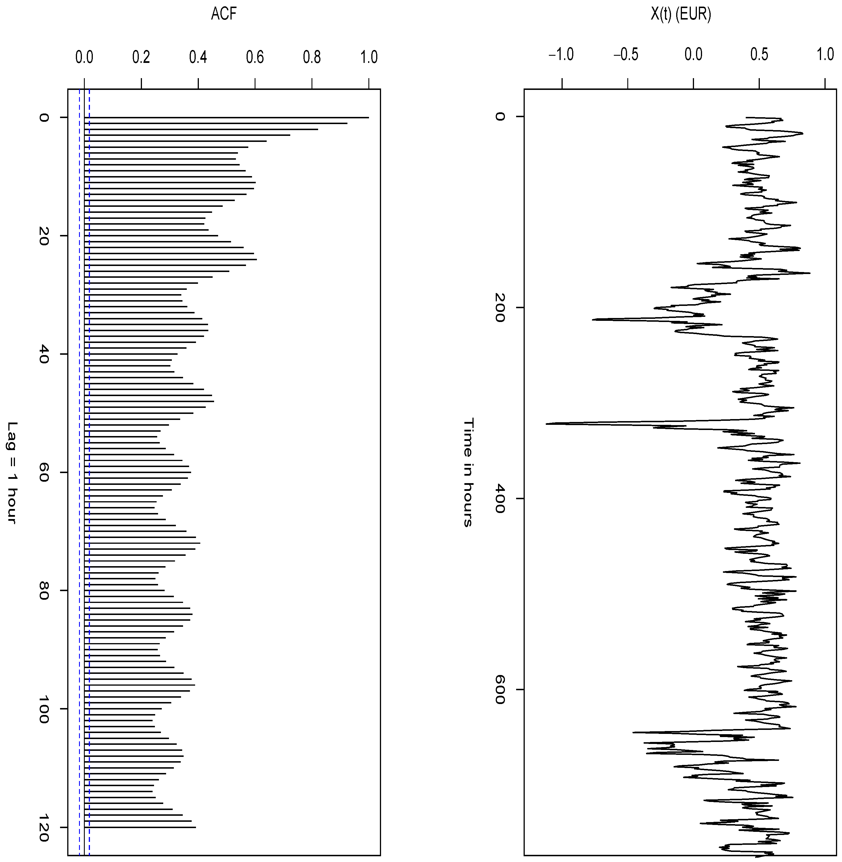
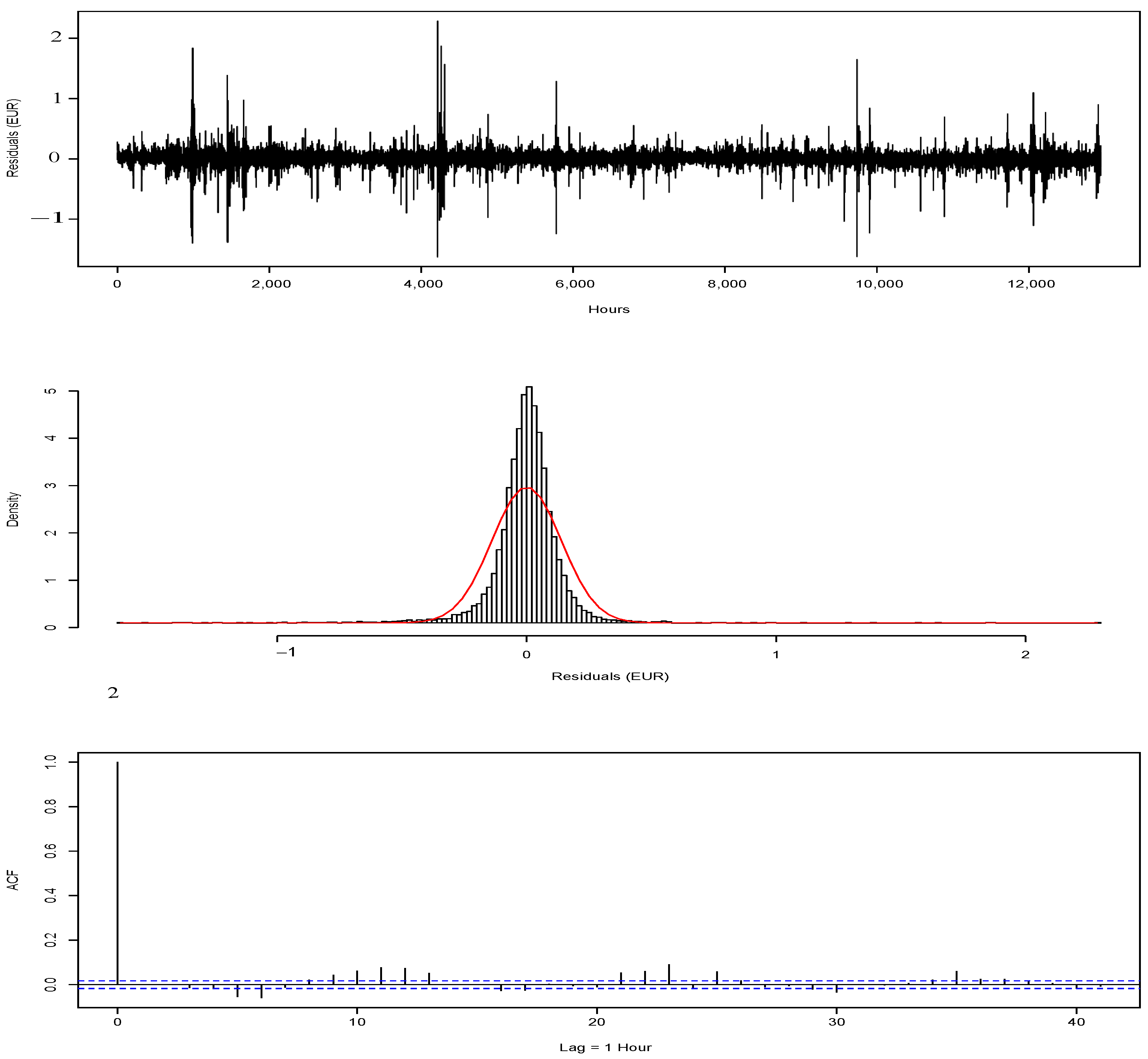
2.2. Statistical Analysis, Model Selection, and Model Fit: Short-Term Stochastic Process
This section is dedicated to the implementation and statistical analysis of the short-term model component. In particular, we look at the theory applied directly to the empirical evidence, and therefore the estimation and best fitting techniques adopted to obtain the best forecast, in our opinion, of the latent variable that describes electricity spot price changes with a short-term period.
The statistical evaluation for parameters was conducted assuming that in Equation (1) (see Burger et al. [7]). Once the PLC was applied, we calculated as
whose sole realization is shown in Figure 2.
Figure 2.
Empirical PLC of the French power market.
Hence, can be understood as the expected value of at each level for any time t. The short-term process , based on the observed data, has a mean value of and a standard deviation of .
Figure 3 displays the solo trajectory during the period 1 January 2016 to 31 January 2016, and the bottom panel depicts the estimated ACF.
Figure 3.
Top panel: the time series of reported for January 2016. Bottom panel: the estimated ACF.
Once we obtained , we searched for a model that could describe changes in the price of short-term electricity. The was computed applying a default smooth spline to the data (we used the default spline present in the ‘R’ software, given by a third-degree polynomial).
From an accurate analysis of the empirical autocorrelation function shown in Figure 3, we note the presence of a strong linear dependence with the 24 h lagged time series. Following the same procedure as the authors of the model, and due to the correlation at the 24th lag, we modeled using a seasonal ARIMA (SARIMA) stochastic process (Brockwell and Davis [24,25]) with a periodicity of 24 h.
Next, we briefly discuss the fitting of the SARIMA process to the short-term latent variable. We note that our short-term process calibration method does not foresee the use of the Kalman filter (Burger et al. [7]), but the standard method is used to obtain the SARIMA model parameters, assuming that in this estimation phase.
The model able to produce a satisfactory result was .
The parameters obtained and reported below aim to maximize the Akaike information criterion (AIC) and log-likelihood function. AIC is the main decision criterion for most of the calibration processes in this study.
Given a time series , we define the backward shift operator as
The model obtained can be represented through characteristic polynomials. If we set , , (with ), the stochastic process can be expressed in the compact form
where denotes white noise with mean of 0 and standard deviation . Therefore, Equation (3) becomes
As mentioned earlier, the decision criterion for estimating the parameters involves the maximization of the log-likelihood function and AIC. The training-set error measures are also reported in Table 1.
Table 1.
Log-likelihood function, AIC, and error measures for the parameter estimation.
Substituting and we can replicate the model obtained from our statistical analysis of the observed data.
Next, a normality test was performed on the estimated residuals of the SARIMA model. The distance between the empirical distribution of the data and the benchmark distribution was estimated using the Kolmogorov–Smirnov test or Kolmogorov distance. In this case, the hypothesized continuous cumulative distribution function is the normal distribution with mean zero and variance . The normality hypothesis is rejected because the p-value is 0, indicating the rejection of the null hypothesis that residuals are drawn from the normal distribution. Moreover, looking at the middle plot in Figure 4, a leptokurtic empirical distribution of is observed.
Figure 4.
Summary of residuals.
We note that the stochastic process (Brockwell and Davis, [24]) considered to be white noise with a mean of 0 and a variance , can be given as
if and only if has a zero mean and autocovariance function :
In contrast, a necessary condition confirms that it is appropriate to verify and study the autocorrelation structure in Equation (5) for residuals.
Hence, a Ljung–Box lack-of-fit hypothesis test was performed. The p-value was larger than 0.05 (0.9359), indicating the absence of autocorrelation among the residuals at the 5% significance level. The above results were confirmed by analyzing the estimated ACF of the residuals in Figure 4.
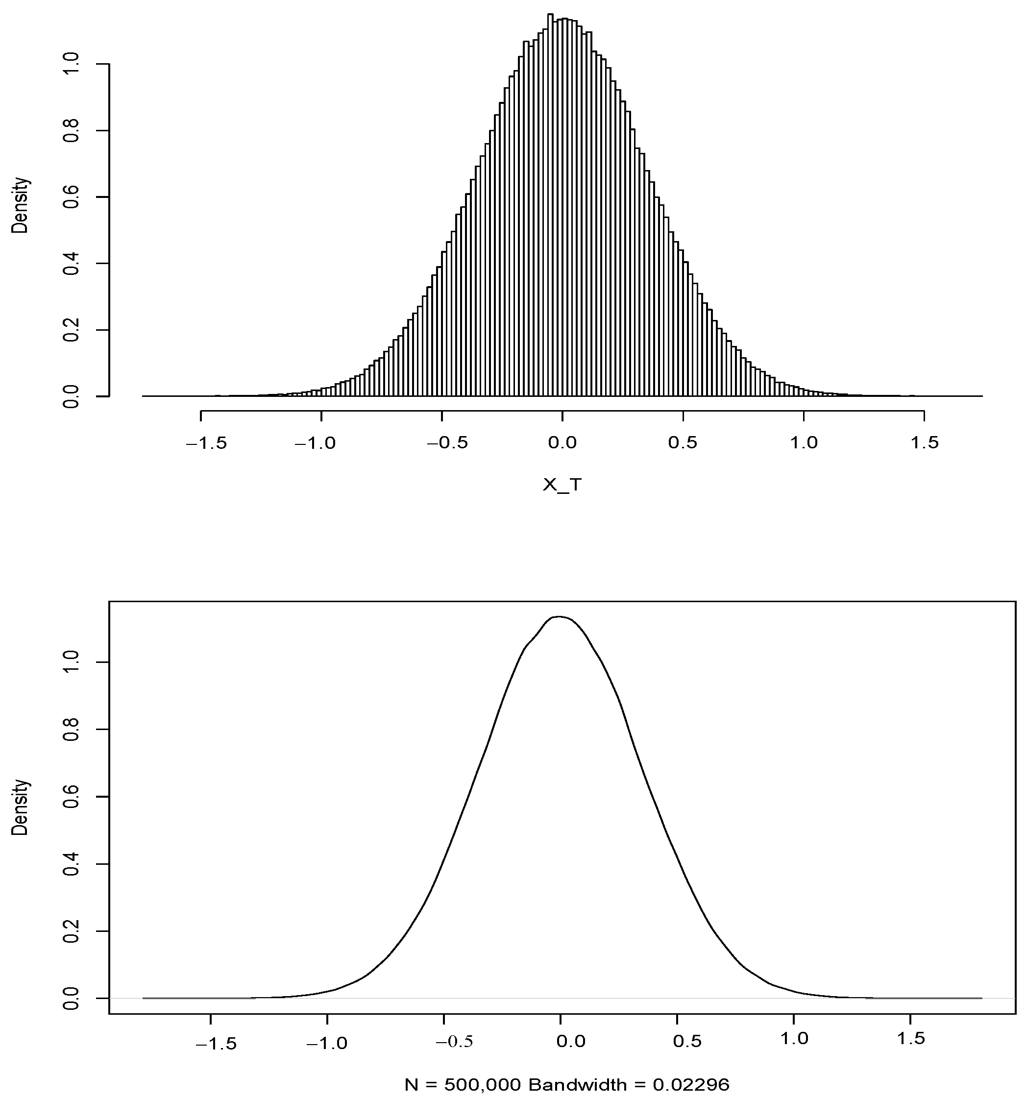
2.3. The Long-Term Process
In Equation (1) of the SMaPS model, the long-term stochastic process follows a random walk with drift
where , is the random walk drift () and are random variables, normally distributed and uncorrelated to each other. Although SMaPS is a discrete model, for this phase it is convenient to consider Equation (6) in terms of its continuous-time definition. In addition, regarding the question of notation in the models present in the financial literature, this is in accordance with the Black model, formulated in 1976, with particular regard to the hypothesis of log-normal distribution applied to futures with underlying electricity for the estimation of volatility .
The continuous-time generalization of Equation (6) is a Brownian motion (see Cont & Tankov, [26]) with drift
(where is the standard Brownian motion).
Next, we switch to an equivalent martingale measure , assuming the market price of risk is zero for the non-hedgeable short-term process and the load process . Further justification of this assumption is given in Burger et al.’s [7] work. Thus, the equation for the long-term process under becomes
where is the new drift, which includes the market price of risk for . Under this new probability measure, futures prices (for single hours) at time t for delivery in T are given by the conditional expectation that
where denotes the -algebra generated by the price process. Assuming zero risk premia for and (see Burger et al. [7], Section 2), we can set the conditional expectation under equal to the natural conditional expectation. At this point, with large enough, we approximate the conditional distributions of and with their stationary distributions. Hence, for the assumption made, it is possible to adopt the following approximations (see Burger et al. [7]):
Neglecting the rounding errors and considering
as the deterministic “technical price”, the single-hour futures prices become
Reorganizing Equation (13) and solving for we obtain the explicit expression
In practice, we can assume that is constant for intervals . Relating to the considered range, its value can then be calculated using a discrete version of Equation (14) as
Long-Term Component Calibration
This calibration involves first estimating the deterministic “technical price”, . According to Equation (12), the following are needed to calculate :
- The SARIMA variance;
- The probability distribution.
Regarding the model, we applied a numerical procedure to obtain , by simulating 500,000 trajectories of the model described. For (152 days), was estimated as . The simulated distribution of is shown in Figure 5.
Figure 5.
The empirical probability distribution of .
To determine the technical price , we need the values of in the future. To present an example that can be replicated in any context, the variable is not treated as an exogenously determined variable, for example, the numerical vector that describes the judgment of the respective department within an electric utility company.
Therefore, we consider a SARIMA model again for 24 h. As was done for , we consider the best SARIMA model capable of maximizing the log-likelihood function (−104,788.6) and AIC (209,593.2). The SARIMA process estimated for the sequence of random variables () which describes the electricity load demanded over time is
and it can be presented in both the compact form
and the extended form. Given , we obtain:
Substituting , , , , , , , and we estimated our model.
Next, by simulating N (with N = 500,000) trajectories of as defined in Equation (16), an estimate according to Equation (10) was obtained using the following estimator:
Calibrating our model by taking the first semester of each calendar year, for days (4320 h), we obtained
and subsequently, using Equation (12), the technical price
The same procedure was repeated for days (5064 h) and the result was
which means €50.34.
The set of parameters required to make Equation (6) operational is complete once we define .
For simplicity, we assume (Burger et al. [7], p. 22) that is constant, thus obtaining an annual drift for the last observation in the sample on 31 December 2018.
To implement the hedging strategy against volumetric risk induced by wind speed, the drift factor for the next 6 months (out-of-sample analysis) was calculated as follows.
Figure 6.
Ticker Bloomberg: ELFBM F20.
Figure 7.
Ticker Bloomberg: ELFBM G20.
In particular, for and , based on the prices in the financial markets, we find a price today for electricity delivery in a year of
and for and ,
From Equation (15), for (month, 31 days, 744 h), the is
Applying the same procedure for additional maturities , we express as a time function. To complicate matters even more, we could further introduce a probabilistic model for , defined by an appropriate stochastic differential equation; however, in this paper, we assume that is constant. Therefore, we observe, in the out-of-sample data in our analysis, a futures contract with underlying electricity and one-year delivery (from the closure of the in-sample data) at a lower price compared with the current contracts observed in the market on 31 December 2018.
From Equation (13) we deduce that , as a function of t, follows a geometric Brownian motion with standard deviation
Assuming (day), and given the sample observed from 2 January 2017 to 31 December 2018 (with T still fixed at 1 January 2020) obtained from the ELFBM F20 OECM Index, we calculate an empirical probability distribution of
which has a standard deviation of on an hourly basis.
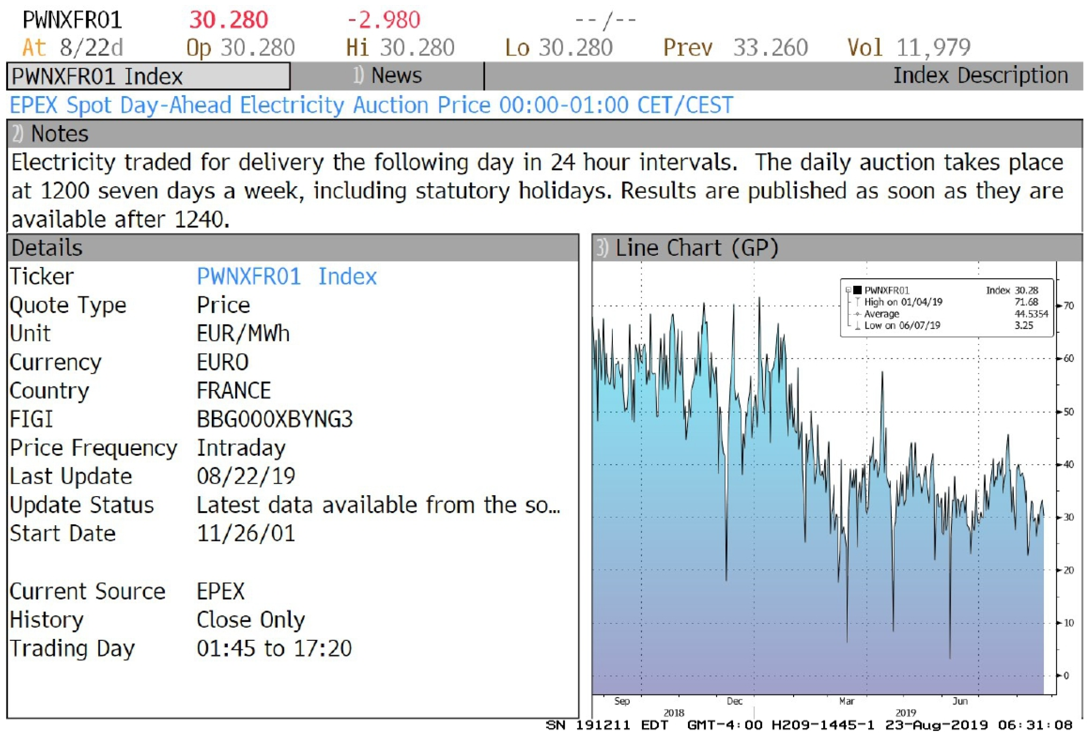
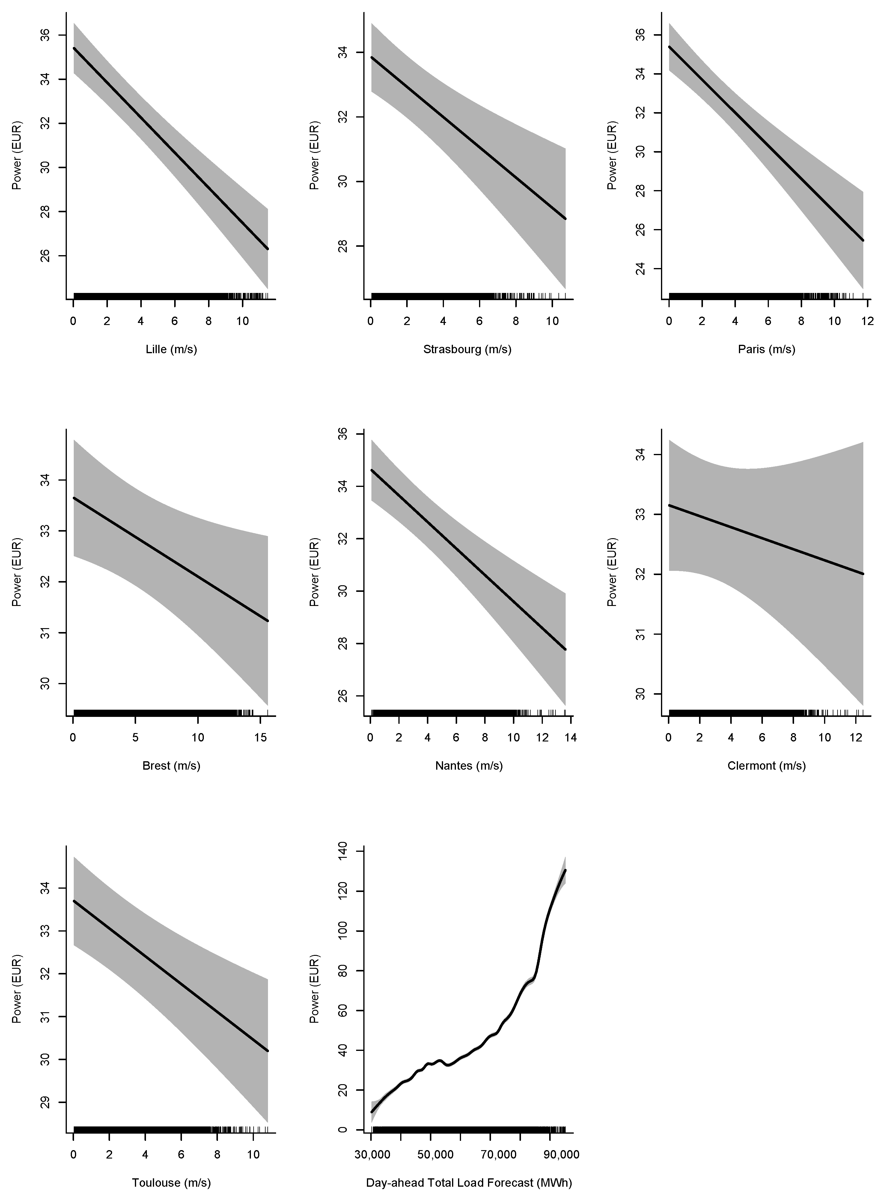
2.4. Statistical Relationship between Wind Speed and the EPEX Spot Day-Ahead Electricity Auction Price in France
Regarding the wind speed series, we used MERRA-2 (https://disc.gsfc.nasa.gov/, accessed on 23 August 2019) to determine the hourly time series for the wind speed. More specifically, we used the two-meter-eastward and two-meter-northward measures (codified as “U2M” and “V2M”, respectively), from which we deduced the two-meter wind intensity. Indeed, altitude from the ground modifies wind speed.
Next, we examined the links between wind speed and spot prices. In a preliminary analysis, we observed a weak linear dependence between standardized spot prices and wind speed. The results of this analysis are shown in Table 2.
Table 2.
Correlation between EPEX spot day-ahead electricity auction price and hourly wind speed (m/s).
In this subsection, we discuss the statistics of wind power price sensitivity to power price in further detail.
Considering the vector as the previous time series of the French spot day-ahead power price and analyzing its conditional distribution, it is evident that a simple linear regression model cannot capture price fluctuations that have a strong daily, weekly, and yearly periodicity. This can be explained from a microeconomic viewpoint by looking at the market price of electricity as the equilibrium price based on supply and demand curves. Since electricity demand is very inelastic, the marginal costs of supply (shown in the merit order curve) determine the price to a large extent. For this reason, we chose a non-parametric function of the day-ahead total load forecast.
Following Engle’s [27] approach, we utilized the following mathematical relationship
which matches the non-parametric regression model. Here, denotes the spot price of power in the day-ahead auction at the hour; is the list of unknown parameters; denotes the day-ahead total load forecast at the hour, and is the wind speed at the hour in the Lille, Strasbourg, Paris, Brest, Nantes, Bordeaux, Clermont, and Toulouse weather stations located in France. Consequently, using the observed sample to estimate the model given by Equation (21), we determine the and that minimize
with . For further explanations regarding the model defined in Equation (22) see, for example, Craven [28] and Engle [27]; for this study, the model is assumed as defined by its authors (obtained computationally with default parameters).
We note that Equation (21) does not describe a relationship with SMaPS. It is introduced to analyze, using another model known from the literature, the relationships between the price of electricity and wind speed. The valuation of the industrial portfolio is undertaken using the SMaPs model only.
Table 3 reports our estimated linear statistics.
Table 3.
Summary of linear components.
By definition, the model’s parametric values are interpreted as partial derivatives of the dependent variable with respect to the various independent variables. Then, we obtain the value of power’s sensitivity to wind speed based on data from the selected weather stations. For example, if the wind speed in Nantes increases by 1 m/s, then we expect a EUR 0.51 reduction in power price plus a margin of error. Figure 8 displays all the regression coefficients and the non-parametric function for the total load.
Figure 8.
Components of the semi-parametric model.
In a more thorough inspection of Figure 8 (part of the semi-parametric model), we observe the empirical merit order curve.
Finally, Figure 9 shows a portion of the model fitted. Due to the strong autocorrelation in the residues shown in Figure 9, the model may not be suitable for forecasting as it overlooks relevant information.
Figure 9.
Top panel: blue line represents the expected value of the model in Equation (21) and black line represents the hourly time series of French power day-ahead auction. Bottom panel: the estimated partial ACF.
3. Industrial Portfolio and Modification of Weather Risk Exposure Using Weather Derivatives
To a large extent, the presence of assets suggests that each entity is capable of economic assessment. In particular, the lack of a harmonized classification allows for the classic distinction between tangible and intangible assets. Tangible assets include land, crops, residential buildings, industries (factories and warehouses), raw materials, etc.
Assets admit the possibility of exchanging monetary amounts available with various time lags (expiration dates) and the nominal/market value endowed. As such, a power plant that generates electric power from both renewable and fossil fuel sources could be interpreted as a tangible asset since it defines a future cash flow characterized by the income from power production and sale.
In this section, we introduce the power industrial portfolio, using market-consistent evaluation criteria because its income is closely linked to all commodity prices quoted on the stock exchange.
Operationally, the market-consistent evaluation of industrial assets serves as the starting point for hedging strategies using suitable financial instruments. This section is organized as follows. In Section 3.1, we examine a hypothetical industrial portfolio of wind farms equipped with real, typical wind turbines (D’Amico, [29]). Next, we determine the empirical probability distribution of the portfolio profit margin in the six months immediately following the date of conclusion of all empirical analyses conducted so far. For this purpose, we introduce the earnings-at-risk as a risk measure in Section 3.2 (Burger, [30]). Lastly, in Section 3.3, we analyze the wind sensitivity of the wind-power industrial portfolio using the scenario shock approach.
3.1. The Wind-Energy-Powered Park Module
Let us consider an enterprise that produces electricity via renewable sources. Previously, the enterprise entered the wholesale electricity business in France by investing in wind-energy-powered park programs. From the perspective of the company’s balance sheet, looking at a hypothetical income statement of a company that only produces renewable energy using wind farms, we develop some hypotheses operationally consistent with the business, characterizing the segment of the energy market under consideration.
Therefore, based on the financial statements of the hypothetical company on 31 December 2018, we assume a negligible cost of goods sold (COGS), and for our analyses, set its value as zero. Thus, the total net sales (as well as revenue) are equivalent to the operating income.
Subsequently, following the format of financial statements, we deduce the general and administrative expenses (G&A) from the operating income to obtain the Earnings Before Interest, Taxes, Depreciation, and Amortization (EBITDA) of the company.
We neglect the COGS results for the possibility of identifying a single source of business uncertainty linked to the company’s revenues. Considering COGS as negligible or equal to zero implies a significant reduction in the firm’s revenue volatility. Reducing uncertainty about the firm’s revenues reduces the EBITDA volatility, which in turn impacts the firm’s present value (intrinsic enterprise value), encouraging investors to enter and capture a share of the renewable energy market, thereby promoting its growth by making it convenient in terms of expected revenues.
The hedging will be significantly weak since the volumetric risk associated with the production of renewable energy is small compared to the market risk. As is known in the markets, the price of electricity, being a secondary energy source, is closely correlated with the price of other commodities such as oil (crude oil, Brent, WTI, etc.), which makes it a source of uncertainty that affects both the company’s revenues (from the sale of the assets) and the COGS.
If all electric utility companies in an area were able to develop new renewable technology capable of overcoming merit order technologies that exploit non-renewable energy, there would be an immediate and significant reduction in revenue variability over time, and consequently in the COGS, consolidating the current value of the company and attracting new investors to the business.
In this practical example, we use a stochastic approach to defining the expected revenues of the company at the time of evaluation, to which we apply the relevant risk measure EaR. Finally, we show how ideal hedging can impact an industrial portfolio with such characteristics.
We first introduce a sequence of random variables , where represents the aggregate revenues at the time , in the balance sheet item “revenue” of the income statement on the relevant closing date. The stochastic variable is trivially given by the product of the price of the good and the quantity demanded , which depends on several factors, at time . The random variable is expressed in monetary amounts (in this case, EUR).
We consider wind turbines located in Paris and Nantes with the following characteristics:
- Hub height of the turbine: 95 m.;
- Rated power of the turbine: 2 MW;
- Cut-in wind speed: 4 m/s;
- Rated wind speed: 13 m/s;
- Cut-out wind speed: 25 m/s.
Specifically, in the French wholesale electricity market context, the authorized department organizes the sale of the amount of energy produced , which is also a sequence of random variables indexed with respect to time.
The net present value (NPV) of this ideal portfolio depends on the time horizon considered in the evaluation since the related industrial assets do not expire like ordinary financial instruments.
To implement a hedging strategy, we utilized a time horizon to define the present value of this portfolio for the horizon considered. In other words, the present value of revenues at , the balance sheet date, for the next k months is a function that is applied to a stochastic process that describes revenues over time using a probabilistic approach.
Therefore, the market value of the revenues of the wind-energy-powered industrial portfolio that generates random positive cash flows is expressed through the pay-off function as
where represents the product of two random variables: the spot price of electricity and the quantity produced and exchanged by individual H wind farms in operation, given by
where is the time frame considered and is the evaluation time.
To complete our example, we consider wind farms located in Paris and Nantes. Under the notation in Burger [30] (p. 127) regarding the definition of the function , and for the assumptions made, i.e., and h, the NPV of the power industrial portfolio for 320 h (six months ending on 1 June 2019) can be defined as
where denotes the power spot price, r indicates the (deterministic continuously compounded) interest rate, represents the function that links wind farm power load (MWh) to the variables that determine it, and Q represents the quantity of energy produced by the wind farm. We estimate the power curve and wind speed observed at time t, expressed in hours, at the weather station , i.e., Paris, Nantes, where are the installed wind power capacities (MW).
Since we plan to estimate the energy produced by a real wind turbine whose hub is at a given altitude, we transform the wind intensity to this specified altitude. The physical law that permits the conversion of wind intensity with respect to altitude is (see D’Amico et al. [29])
where represents the wind speed measured at the height h of the wind turbine hub and is the known value of the wind speed at the specified height (here, m). Furthermore, the parameter is a factor directly linked to the morphology of the site surrounding our hypothetical wind turbine. For example, if the area has no buildings or trees, this parameter ranges typically from to , whereas for offshore applications, this parameter is equal to . In this survey, we take a mean value for an onshore application of . Given this transformation, the main statistics of the wind intensity at the desired altitude are then modified. The next step is to determine the energy produced by the turbine. It is well known that wind turbines transform the kinetic energy of wind into electrical power due to the rotational movement of the blades. The amount of energy produced depends not only on wind intensity but also on the characteristics of the blades. For this purpose, the turbine is characterized by the power curve, which represents the amount of energy produced based on wind intensity. In general, the power curve is linked to two critical values for wind speed. Below the first threshold (cut-in value), the blades do not produce energy (the kinetic energy of the wind is too weak to move them). Above the second threshold (cut-out value), the system is blocked to avoid structural damage. Between these two thresholds, there is a polynomial relation (known as the Betz law) between wind speed and energy produced (see [29]). In our survey, we applied the following power curve:
Note that the wind speed obtained in Equation (26) must be inserted into Equation (25) instead of .
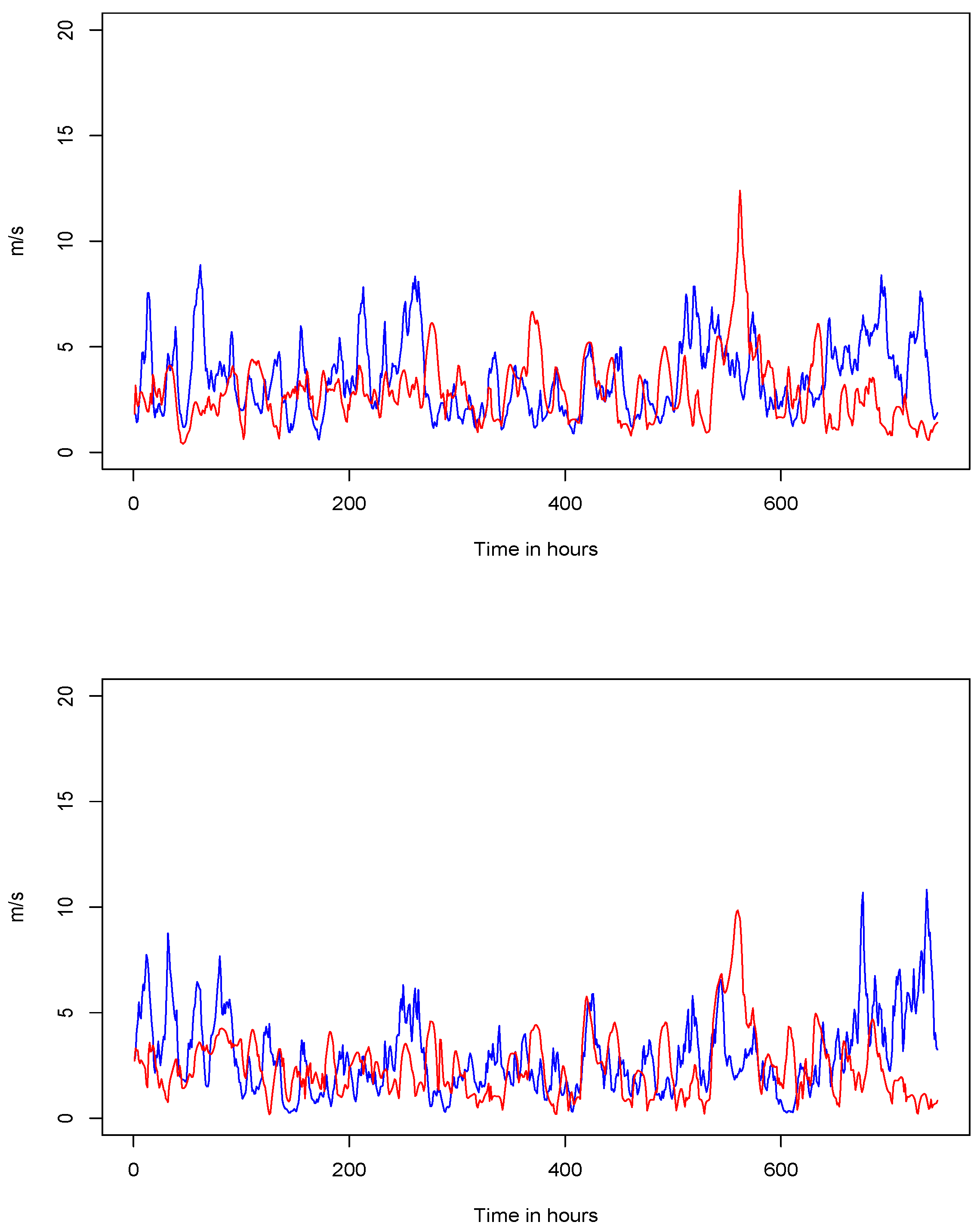
Wind Speed Stochastic Modeling
In this subsection, we briefly introduce the main models used to represent the wind speed series. Let be a time series and be a function of time and exogenous variables. An extended pure SARIMA model for (Brockwell and Davis [24], McLeod [31]) can be expressed with the help of the backward shift operator as
where represents white noise, and , , and are polynomials, such that all roots of are in the unit circle, while the roots of and are outside the unit circle. If the unit roots are missing, the model is stationary with a mean of zero. The SARIMA model can be represented in an equivalent form as
where . This process (Brockwell and Davis [24]) is said to be causal (or more specifically, to be a causal function of if there exists a sequence of constants such that and
Causality is equivalent to the condition
A SARIMAX model can be defined as a regression with SARIMA residuals
where is the centered . This can be written equivalently as a single equation
whereas the regression function can depend on time and/or (possibly lagged) exogenous variables.
First, we use simple regression to investigate and capture the linear dependence between the Paris (dependent variable) and Nantes (independent variable) wind speed time series (note that is associated with Paris and with Nantes), whose results and goodness of fit are shown in Table 4. Using the fitted values , obtained from the regression model applied to the two historical in-sample wind series, we define the residual Paris wind speed time series as
Table 4.
Main features of the Nantes SARIMA model.
We again use a seasonal ARIMA to model . At least, the has the expression
which is the best-fitting seasonal ARIMA model based on the values of Akaike’s information criterion (−6776.99) and the Bayesian information criterion (−6736.1).
In Figure 10 we display two simulated paths of the Nantes (using SARIMA) and Paris (using SARIMAX) models compared with the out-of-sample real wind speed time series. It is evident that to depict variation in the regressors, we need to develop a simulation model for the Nantes wind speed. All the features of the wind speed models are presented in Table 4 and Table 5, which show the Box–Cox transformed data.
Figure 10.
Overhead, hourly Nantes wind speed (red line) vs. simulation path (blue line), followed by hourly Paris wind speed (red line) vs. simulation path (blue line) for the period 1 January–1 February 2019.
Table 5.
Main features of the Paris SARIMAX model.
According to the modeling techniques used in previous literature (Benth et al. [18], Alexandridis et al. [6]), we make the wind speed time series symmetrical with respect to . To this end, we use the Box–Cox transformation defined as
where parameter l is estimated by maximizing the log-likelihood function. The parameter is the more likely value, compared to the values that can be assumed based on the observed data, such that the empirical distribution becomes symmetrical.
In particular, to measure the goodness of fit of the models, we report the mean error (ME), the mean square error (MSE), the RMSE, the MAE, the MAPE, and the MASE of the models fitted. MAPE is the most common measure used to forecast error and to determine the comparative accuracy of forecasts as a function of loss, in order to select the best model.
3.2. Earnings-at-Risk and Wind Sensitivity
According to Burger et al. [30], spot prices are much more volatile than forward prices, especially for commodities that cannot easily be stored. For this reason, the distribution of spot prices is often heavy-tailed and the assumption of a log-normal distribution is inadequate. In this subsection, we use a scenario approach to obtain the probability distribution of the wind-powered industrial portfolio market value (its NPV, using a market-consistent approach) described by Equation (25).
Next, we simulate every source of risk for the next semester using the newly constructed model. The sources of risk include volumetric risk due to wind speed fluctuations, which affect energy production indirectly, and market risk, which depends on variations in wholesale electricity prices.
Specific risk measures such as profit-at-risk, earnings-at-risk (EaR), and cash-flow-at-risk are used to integrate spot market risks and thus provide an additional view regarding portfolio risks.
In our introductory example, our ultimate goal is to define the probability distribution of aggregate revenues for the next s hours, in the first instance, and then to introduce an appropriate risk measure. We defined (Burger [30], p. 127) EaR as the difference between the expected value of the revenues and the revenues, corresponding to a given confidence level. For energy companies, this includes spot price revenues generated by assets, less all production costs, plus all related trading and hedging transactions. To calculate the EaR, we used the Monte Carlo method. Since EaR characteristics are in line with our research purpose, we adopted the EaR as a risk measure.
Following De Felice and Moriconi ([32], p. 66), for a given probability level (i.e., %), we define the worst-case value of as the alpha-quantile of the probability distribution of . Therefore, the level of is a pessimistic value of the revenues. In other words, this is the estimated amount at of possible future revenues reduction, such that lower values can occur with a probability level .
Hence, the EaR, conditioned to the filtration available at is given by
The EaR expresses the maximum potential loss to security at the level. The procedure used to obtain the quantity in Equation (29) involves the following simple steps. First, we use the SMaPS to simulate the hourly spot power price scenarios in the next (out-of-sample) six months. Then, we simulate the hourly wind speed in the same way and obtain the load scenario from the power curve. In the EaR definition, we omit the time decay factor, the Solvency II standard formula.
Based on the models previously obtained, we simulated 100,000 paths of the spot French market power price and 100,000 paths of the hourly wind speed in Nantes and Paris over the next semester (out-of-sample), from 00:00 1 January 2019 to 23:00 2 August 2019 . More specifically, we let () be the simulated trajectories,
the Monte Carlo estimate of the conditional expected value in Equation (29), and the -quantile of the estimated density. Therefore, ultimately, we estimate the empirical EaR by
We depict a worst-case (with a probability level of ) portfolio value, EUR 20,609,424, and the EaR = EUR 19,365,410. The empirical density is given in Figure 11.
Figure 11.
Industrial portfolio market value empirical probability distribution.
3.3. Scenario Approach for Wind Sensitivity
It is crucial to develop a common hedging strategy against wind speed fluctuations and their impact on the profit margin variations in the power portfolio. As a working hypothesis, additive shifts are considered for the value of a portfolio that is affected by infinitely small fluctuations in wind speed:
Recalling the working hypotheses, we consider two wind farms located in Nantes and Paris. Consequently, we measure the two differentiated wind risk exposures for single geographical positions as
Thus, with all other variables that contribute to the definition of the portfolio value being equal, the portfolio market value is calculated as
where is the random amplitude of the shift caused by . Hence, the wind speed risk exposures become (with )
measured in EUR/. In Equation (32), the portfolio value is a random variable. It will be adopted as a summary index of the distribution of , the sample mean of the empirical probability distribution obtained in the Section 2. The additive shift in Equations (30) and (31) occurs for fluctuations in both wind energy production and wind speed. Following the analysis conducted in Section 1, there is an average decrease of EUR −0.005 per increase (all other conditions being equal) in the wind speed recorded at Nantes. Based on these results, we decided to ignore price fluctuations due to wind speed.
To obtain a numerical estimation of Equation (32), the wind speed scenarios are generated again by applying a shift on the trajectories of the wind models previously used. Next, the Monte Carlo estimations for are given as
In summary, the risk exposures (wind speed risk) inherent in the wind generation parks are estimated as
In particular, based on the 100,000 simulations with the horizon considered before, we estimate a risk exposure of EUR 14,398,437 and EUR 20,490,884 for the wind farms located in Paris and Nantes, respectively. Additionally, we calculate an hourly risk exposure of EUR 2803.98 and EUR 3990.44, for Paris and Nantes, respectively.
4. Validation of the Delta Hedging Strategy Performance
To complete our analysis, and in terms of modern risk management, one last step is necessary, i.e., determining the modification in risk exposure. Weather derivatives are financial instruments that can be issued by organizations or individuals as part of a risk-management strategy to reduce the inherently harmful and unforeseen consequences associated with adverse weather conditions (with respect to economic operations). In finance, a weather derivative is a contract whose price is based on a physical measure (air temperature, atmospheric precipitation, humidity, wind speed, etc.) observed at a specific meteorological station. Users of derivatives, as part of their strategy to hedge portfolio risks, can efficiently eliminate the risk associated with adverse weather conditions. First, the low volatility of company profits reduces the risk of large losses and bankruptcy. Second, it reduces the volatility of the hypothetical company’s stock prices, along with an increasing prices trend. The weather derivative is regulated financially using the pay-off function. The pay-off defines precisely who and how much to pay on the contract due dates.
In line with the notation used in (Jewson and Brix, [8]), we consider a collar option. A long position on a collar is a combination of a long position on a call option and a short position on a put option with the same underlying features but, usually, different strikes and limitations. A long position on a collar option defines a type of pay-off function as
or equivalently,
where x denotes the wind speed at the given station, and are the limits agreed on monetary disbursements, and are the fixed strikes (m/s), and represents the ticks.
4.1. Contract Issuing Phase
We assume the existence of two over-the-counter financial instruments with an underlying wind speed that allows the company to cover itself in case of expected reductions in revenues caused by a drop in electricity production due to low wind speed.
The division agrees with the counterpart by purchasing financial protection defined through two structured contracts and , each equivalent to a portfolio of collar options with expiry , hedging against the small values of wind speed that were registered every hour from 1 January 2019 to 2 August 2019.
The underlying factor chosen by the two counterparts is the meteorological observation referred to Paris and Nantes in relation to the registered wind speed .
In this case, the two counterparts agree to exchange a random monetary amount every hour based on surveys of meteorological stations conducted with respect to contractually established conditions. It is possible to express mathematically the monetary result of the two structured contracts purchased by the company as follows
for the hours following the protection: , with the wind speed expressed in m/s. The slopes of the lines that describe the pay-offs of the collars are the risk exposures determined previously, while the other parameters are arbitrary and may depend, in reality, also on contractual factors. The coverage cost at will be equal to (assuming the hypothesis of a constant and deterministic risk-free interest rate ):
where the transformation of the stochastic wind process into the risk-neutral probability measure is a non-trivial operation. We show in Figure 12 the pay-off of the collar option , which is similar to the collar option .
Figure 12.
Pay-off of the collar option .
4.2. The Hedging Strategy and Its Impact on Risk Measures
After the purchase of the two structured contracts, the stochastic industrial portfolio value at becomes
At this point, retracing the steps mentioned in Section 4.1, we estimate the probability distribution of and recalculate all its respective risk measures. The hedging strategy implemented implies that the new worst-case value appears to be EUR 29,306,880, with an improvement of compared to the portfolio’s EUR 20,609,424 without the two structured financial instruments. Similarly, the overall EaR of the portfolio is now valued at EUR 18,137,476, with a reduction compared to the previous EaR without the two structured contracts. This phenomenon is justified through the high electric price volatility, compared to the many variables now common in the literature that contribute to the peculiar variance of the hourly price of electricity.
Figure 13 shows the empirical probability distribution of thus obtained. Finally, Table 6 shows the partial matrices for space purposes, which contain the results of the Monte Carlo simulations. Each matrix shows the initial and intermediate values needed to define the empirical probability distribution of first, and subsequently . Moreover, Figure 14 shows the first two trajectories simulated using the SARIMAX model, to which the power curve (the figure in the middle) was applied, together with the first trajectory of the electricity price simulated using the SMaPS model.
Figure 13.
Empirical probability distribution of .
Table 6.
Density profit margin evaluation before and after hedging strategy, using spot price and load scenarios for the 5135 single hours of the front year.
Figure 14.
From the top down: two simulated trajectories of the wind speed of Paris and Nantes cross-correlated with each other (), which enter the power curve. Lastly, a simulated trajectory of the spot electricity price in France. Each simulation refers to the time horizon from 1 January 2019 to 2 August 2019.
The proposed hedging strategy is applicable in a professional environment for several reasons. First, there is a strong information asymmetry between the two parties entering the financial transaction. The counterpart, which can be any investment bank, with its valuations, estimates adverse climatic conditions for the next six months (e.g., a colder winter than normal) and therefore considers our coverage to be advantageous. If this were the case, monetary disbursement from the financial sector would be compensated by the industrial one because, in adverse weather conditions, wind farms are able to produce more energy (with variable costs close to zero) without the use of, e.g., thermoelectric power plants (or buying energy from another supplier) to satisfy demand. For this reason, the critical aspect of the entire industrial risk management process lies in the precision of the calculation. Therefore, sophisticated techniques aimed at defining risk exposure as precisely as possible must be used, in order for the adopted strategy to be considered valid.
5. Conclusions
Weather risk can lead to significant losses in industrial activities. This risk has received considerable attention via the development of adequate financial products aimed at reducing the risk of losses arising from adverse weather conditions to a certain extent. In this study, we addressed the production of electricity in a wind farm. In this case, connected activities can suffer losses due to a decrease in the intensity of the wind because, for a company that produces wholesale electricity, the insufficiency of the supply of energy produced by the movement of air masses to meet the demand may result in increased variable costs induced by the exploitation of non-renewable production sources, i.e., the standard scheme of the merit order curve, which foresees the succession preference for nuclear energy, lignite, coal, gas power stations, and gas turbines. The two main stochastic variables considered in this study were wind speed and the price of electricity. Wind speed was modeled using typical econometric models, while electricity price was modeled using the SMaPS model developed by Burger et al. [7].
The two models were then simulated independently of each other. Our hypothesis found justification by applying Engle’s model to formally characterize the relationship between electricity price and wind intensity. Furthermore, we found that the changes in price due to wind speed were negligible. For the management of an industrial portfolio, we observed that developing a common hedging strategy against fluctuations in wind speed could cause a slightly significant reduction () in the variability of revenues if this was measured by the EaR, which includes two weather derivatives. In contrast, we also observed a improvement in the worst-case scenario compared to the previous portfolio.
We considered a practical application based on data relating to the French market (hypothetical wind farms located in Nantes and Paris), from which we estimated all the models’ parameters. In particular, we utilized a collar option. Through a hedging strategy, we compared the characteristics of a particular industrial portfolio with and without hedging. Regarding the hedged portfolio, we observed that the “worst value” increased considerably, while the EaR decreased.
Incidentally, it should be noted that the value of the portfolio contains the coverage cost and consequently can be arbitrarily modified based on the definition of the pay-off used. However, we used a derivative with contractual conditions established at the outset, and therefore we did not face the problem of establishing the price variation of the portfolio based on the structure of the hedging derivative used.
These considerations, which represent an innovative aspect of our study, are only in relation to volumetric risk management (Roncoroni et al. [9]), thus neglecting the market risk associated with electricity price volatility, allowing us to conclude that the hedging operation of our industrial portfolio provides substantial benefits in terms of the worst-case scenario, for which the application of weather derivatives certainly helps to dampen losses arising from unfavorable weather events.
It should be noted that there are many types of weather derivatives (since they are linked to the structure of related pay-offs). With this in mind, we could analyze the performance of different types of derivatives in subsequent studies. Another future contribution could be the introduction of a stochastic and no-longer-deterministic interest rate structure.
Author Contributions
The authors contributed equally to this work. More specifically, G.M. and M.M. followed the conceptualization and A.R. developed the algorithms necessary for numerical processing. All authors have read and agreed to the published version of the manuscript.
Funding
This research received no external funding.
Conflicts of Interest
The authors declare no conflict of interest.
Abbreviations
| spot price of electricity | |
| energy load process | |
| short-term process for the SMaPS model | |
| long-term process for the SMaPS model | |
| price load curve | |
| average relative availability of power plants (not used) | |
| backward shift operator | |
| typical white noise | |
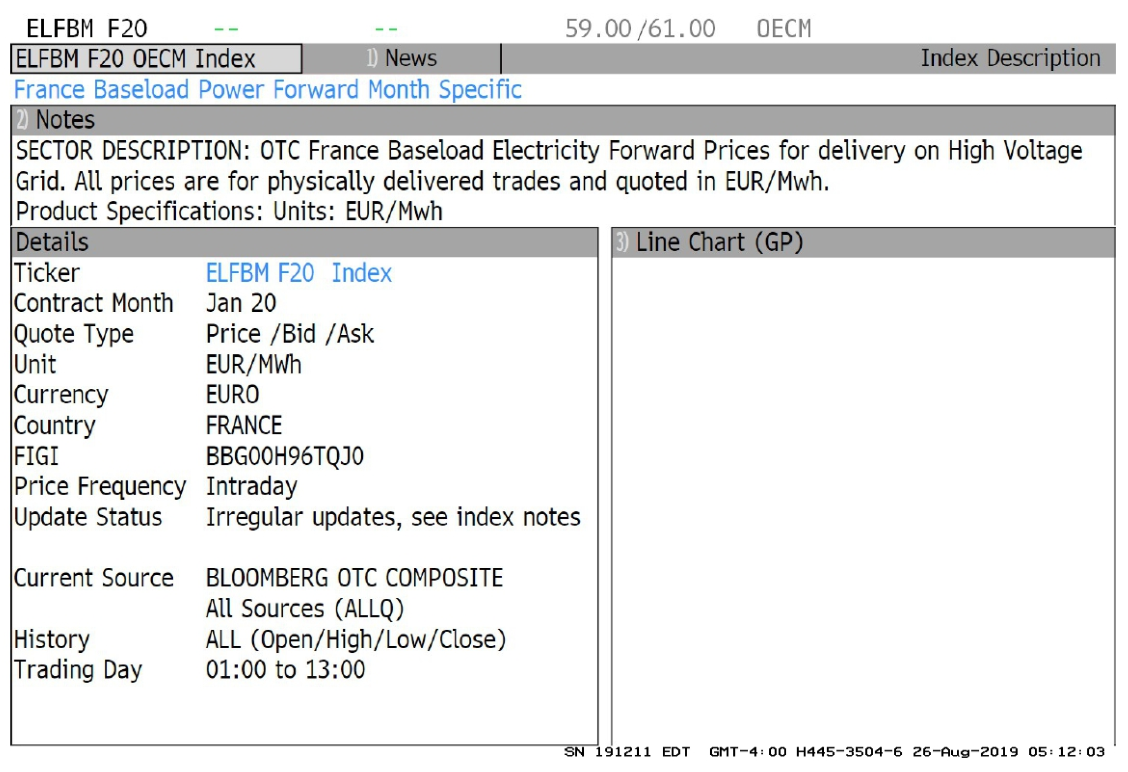
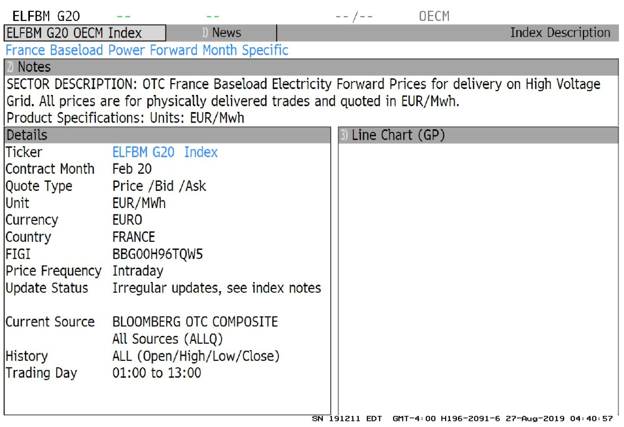
| futures price, at time t, of a contract that foresees delivery of 1 MWh at time | |
| wind speed at time i for station z | |
| aggregate revenue of the power company | |
| energy produced by wind plant | |
| power curve | |
| NPV of the industrial portfolio | |
| installed capacity of a wind plant | |
| earnings-at-risk | |
| , () | exposure to wind risk |
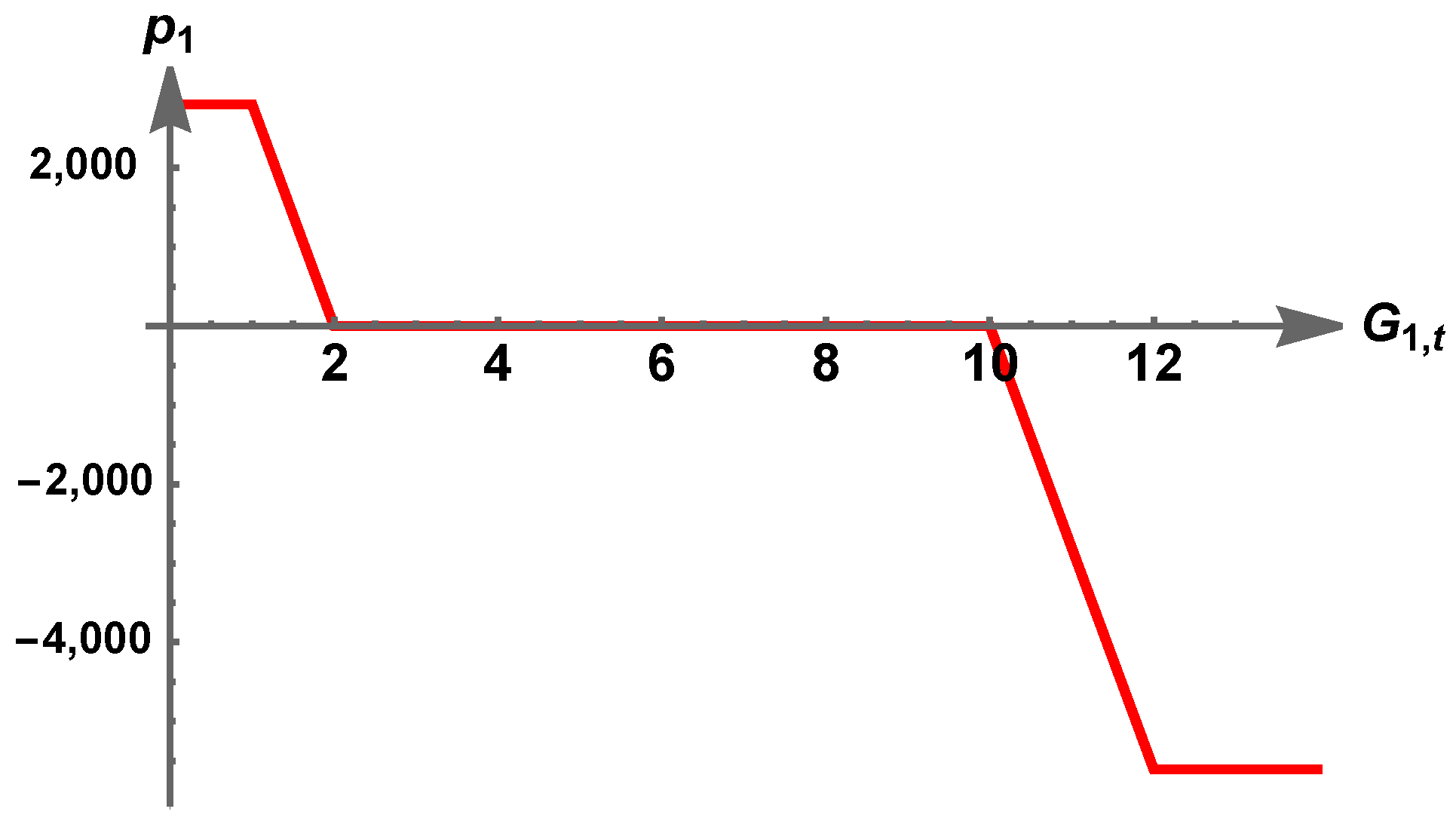
| pay-off of a long collar | |
| coverage cost in t of the structured contract |
References
- Muller, A.; Grandi, M. Weather Derivatives: A Risk Management Tool for Weather-sensitive Industries. Geneva Pap. Risk Insur. 2000, 25, 273–287. [Google Scholar] [CrossRef]
- Pérez-Gonzalez, F.; Yun, H. Risk Management and Firm Value: Evidence from Weather Derivatives. J. Financ. 2013, LXVIII, 2143–2176. [Google Scholar] [CrossRef]
- Salgueiro, A.M.; Tarrazon-Rodon, M.A. Weather derivatives to mitigate meteorological risks in tourism management: An empirical application to celebrations of Comunidad Valenciana (Spain). Tour. Econ. 2021, 27, 591–613. [Google Scholar] [CrossRef]
- Stulec, I.; Petljak, K.; Bakovic, T. Effectiveness of weather derivatives as a hedge against the weather risk in agriculture. Agric. Econ.-Czech. 2016, 62, 356–362. [Google Scholar] [CrossRef] [Green Version]
- Dawkins, L.C. Weather and Climate Related Sensitivities and Risks in a Highly Renewable UK Energy System: A Literature Review; Crown Copyright, Met Office, Exeter (UK): London, UK, 2019. [Google Scholar]
- Alexandridis, A.K.; Zapranis, A.D. Weather Derivatives, Modeling and Pricing Weather-Related Risk; Springer: New York, NY, USA, 2013; ISBN 978-1-4614-6070-1. [Google Scholar]
- Burger, M.; Klar, B.; Muller, A.; Schindlmayr, G. A spot market model for pricing derivatives in electricity markets. Quant. Financ. 2004, 4, 109–122. [Google Scholar] [CrossRef]
- Jewson, S.; Brix, A. Weather Derivative Valuation: The Meteorological, Statistical, Financial and Mathematical Foundations; Cambridge University Press: Cambridge, UK, 2005; p. 392. [Google Scholar]
- Roncoroni, A.; Fusai, G.; Cummins, M. Handbook of Multi-Commodity Markets and Products: Structuring, Trading and Risk Management; John Wiley & Sons, Ltd.: Hoboken, NJ, USA, 2015; pp. 255–277. [Google Scholar]
- Alaton, P.; Djehiche, B.; Stillberger, D. On Modelling and Pricing Weather Derivatives. Appl. Math. Financ. 2002, 9, 1–20. [Google Scholar] [CrossRef]
- Cui, K.; Swishchuk, A. Applications of Weather Derivatives in Energy Market. J. Energy Mark. 2015, 8, 59–76. [Google Scholar] [CrossRef]
- Fernandes, G.; Lima Gomes, L.; Teixeira Brandão, L.E. Mitigating Hydrological Risk with Energy Derivatives. Energy Econ. 2019, 81, 528–535. [Google Scholar] [CrossRef]
- Barucci, E.; La Bua, G.; Marazzina, D. On relative performance, remuneration and risk taking of asset managers. Ann. Financ. 2018, 14, 517–545. [Google Scholar] [CrossRef] [Green Version]
- Lee, Y.; Oren, S.S. A multi-period equilibrium pricing model of weather derivatives. Energy Syst. 2010, 1, 3–30. [Google Scholar] [CrossRef] [Green Version]
- Bressan, G.M.; Romagnoli, S. Climate risks and weather derivatives: A copula-based pricing model. J. Financ. Stab. 2021, 54, 100877. [Google Scholar] [CrossRef]
- Kanamura, T.; Homann, L.; Prokopczuk, M. Pricing analysis of wind power derivatives for renewable energy risk management. Appl. Energy 2021, 304, 117827. [Google Scholar] [CrossRef]
- Benth, F.E.; Lange, N.; Myklebust, T.A. Pricing and hedging quanto options in energy markets. J. Energy Mark. 2015, 8, 1–35. [Google Scholar] [CrossRef]
- Benth, F.E.; Di Persio, L.; Lavagnini, S. Stochastic modeling of wind derivatives in energy markets. Risks 2018, 6, 56. [Google Scholar] [CrossRef] [Green Version]
- Caporin, M.; Preś, J.; Torro, H. Model based Monte Carlo pricing of energy and temperature Quanto options. Energy Econ. 2012, 34, 1700–1712. [Google Scholar] [CrossRef] [Green Version]
- Benth, F.E.; Ibrahim, N.A. Stochastic modeling of photovoltaic power generation and electricity prices. J. Energy Mark. 2017, 10, 1–33. [Google Scholar] [CrossRef] [Green Version]
- Rodríguez, Y.E.; Pérez-Uribe, M.A.; Contreras, J. Wind Put Barrier Options Pricing Based on the Nordix Index. Energies 2020, 14, 1177. [Google Scholar] [CrossRef]
- Kaufmann, J.; Kienscherf, P.A.; Ketter, W. Modeling and Managing Joint Price and Volumetric Risk for Volatile Electricity Portfolios. Energies 2020, 13, 3578. [Google Scholar] [CrossRef]
- Wieczorek-Kosmala, M. Weather Risk Management in Energy Sector: The Polish Case. Energies 2020, 13, 945. [Google Scholar] [CrossRef] [Green Version]
- Brockwell, P.J.; Davis, R.A. Time Series: Theory and Methods, 2nd ed.; Springer Series in Statistics; Springer: New York, NY, USA, 1991; p. 580. [Google Scholar]
- Brockwell, P.J.; Davis, R.A. Introduction to Time Series and Forecasting, 2nd ed.; Springer: New York, NY, USA, 2002; p. 437. [Google Scholar]
- Cont, R.; Tankov, P. Financial Modelling with Jump Processes; CRC Press LLC: Boca Raton, FL, USA, 2004; p. 528. [Google Scholar]
- Engle, R.F.; Granger, C.W.J.; Rice, J.; Weiss, A. Semiparametric Estimates of the Relation between Weather and Electricity Sales. J. Am. Stat. Assoc. 1986, 81, 310–320. [Google Scholar] [CrossRef]
- Craven, P.; Wahba, G. Smoothing noisy data with spline functions: Estimating the correct degree of smoothing by the method of generalized cross-validation. Numer. Math. 1979, 31, 377–403. [Google Scholar] [CrossRef]
- D’Amico, G.; Petroni, F.; Prattico, F. Wind speed prediction for wind farm applications by Extreme Value Theory and Copulas. J. Wind. Eng. Ind. Aerodyn. 2015, 145, 229–236. [Google Scholar] [CrossRef]
- Burger, M.; Graeber, B.; Schindlmayr, G. Managing Energy Risk. A Practical Guide for Risk Management in Power, Gas and Other Energy Markets; John Wiley & Sons, Ltd.: Hoboken, NJ, USA, 2014; p. 439. [Google Scholar]
- McLeod, A.I.; Yu, H.; Krougly, Z. Algorithms for Linear Time Series Analysis: With R Package. J. Stat. Softw. 2007, 23, 1–26. [Google Scholar] [CrossRef] [Green Version]
- De Felice, M.; Moriconi, F. Una Nuova Finanza D’Impresa; Il Mulino: Bologna, Italy, 2011; Volume 196. [Google Scholar]
Publisher’s Note: MDPI stays neutral with regard to jurisdictional claims in published maps and institutional affiliations. |
© 2022 by the authors. Licensee MDPI, Basel, Switzerland. This article is an open access article distributed under the terms and conditions of the Creative Commons Attribution (CC BY) license (https://creativecommons.org/licenses/by/4.0/).