Support Vector Quantile Regression for the Post-Processing of Meso-Scale Ensemble Prediction System Data in the Kanto Region: Solar Power Forecast Reducing Overestimation

Abstract

Although the recent development of solar power forecasting through machine learning approaches, such as the machine learning models based on numerical weather prediction (NWP) data, has been remarkable, their extreme error requires an increase in the amount of reserve capacity procurement used for the power system safety. Hence, a reduction of the serious overestimation is necessary for efficient grid operation. However, despite the importance of the above issue, few studies have focused on the model design, suppressing serious errors, to the best of the authors’ knowledge. This study investigates a prediction model that can reduce the huge overestimation of the solar irradiance, which poses a risk to the power system. The specific approaches used are as follows: the employment of Support Vector Quantile Regression (SVQR), the utilization of Meso-scale Ensemble Prediction System (MEPS, Meso-scale EPS for the regions of Japan) data, which is based on the forecasts from Meso-scale Model (MSM) as explanatory variables, and the hyperparameter adjustment. The performance of the models is verified in the one day-ahead forecasting for surface solar irradiance at five sites in the Kanto region as the numerical simulation, where their forecasting errors are measured by the root mean square error (RMSE) and the 3$\sigma$ error, which corresponds to the 99.87% quantile error of the order statistics. The test results indicate the following findings: the SVRs’ RMSE and 3$\sigma$ error tend to be trade-offs in the case of varying the penalty of the regularization term; by using SVR as a post-processing tool for MSM or MEPS data, both of the score of their metrics can be improved from original data; the MEPS-based SVQR (MEPS-SVQR) could provide superior performance in both metrics in comparison with the MSM-based SVQR (MSM-SVQR) if the parameters are properly adjusted. Although the time period and the type of MEPS data used for the validation are limited, our report is expected to help the design of NWP-based machine learning models to enable short-term solar power forecasts with a low risk of overestimation.

1. Introduction

Among the renewable energy sources, variable renewable energies (VRE) such as photovoltaic (PV) and wind power have significantly increased their installed capacity. The IEA’s 2020 analysis (the main scenario case) predicted that their installed capacity will exceed that of coal-fired power plants in 2024 [1], and furthermore, its 2021 analysis predicts that their installation will be accelerated further than the 2015–2020 period on average due to policy support in each country [2]. However, the power generation of VRE is unstable because it depends on weather conditions. Thus, forecasting techniques for wind speed and solar irradiation are important for the stable operation of a low emission power system with large amounts of VRE.

The participation of VRE in the electricity market causes an imbalance risk to the contracted power supply in the spot market (the day-ahead market). As a hedge against imbalance risk, many electricity markets include a balancing market in addition to the intra-day market. Although the details of the balancing market differ among the EU countries where electricity markets were implemented earlier [3], they share a common framework [4,5].

• Balance responsible parties (BRPs) submit supply/demand plan to the system operator (SO) and work towards meeting the same amount of the plan through the use of the intra-day market;
• The SO is ultimately responsible for the imbalance of the BRPs after the gate close (GC), and procures power from the balance service providers (BSPs) for adjustment before the day before the GC in order to deal with it;
• BSPs activate their regulating power upon receiving orders from the SO when imbalance occurs in the actual section.

What is important to note in the above, is that the SO needs to bid for regulated power from the BSP at least one day before the actual demand supply. In other words, the SO needs to procure regulating power to cope with the uncertainty of VRE generation by the forecast from the previous day or earlier.

In determining the capacity of the balancing services to cope with imbalance risk, ENTSO-E has required SOs in the European union since 2017 to statistically process the uncertainty (such as demand and VRE forecast errors) and estimate the amount of the frequency restoration reserves (FRRs) to achieve a high level of reliability [6]. (See [7] for more recent development). As an example, the Graf-Haubrich method used in Germany constructs a probability distribution function (PDF), which takes into account all important factors of imbalance, such as power plant outages, load variations, forecast errors, etc., and calculates the necessary control reserves including the tertiary control reserve (TCR) corresponding to a specified percentile of the PDF in order to maintain a certain security level [8]. Probabilistic solar power forecasting has been studied by many researchers for efficient reserve power procurement [9], on the other hand, there is also the case where simple schemes that use extreme errors in historical data for reserve power procurement is adopted. In Japan, the Ministry of Economy, Trade and Industry (METI) has held discussions on the balancing market, and considers that the amount of regulating power to be procured by the SO should be equivalent to 3$\sigma$ error, which corresponds to the 99.87% quantile of the historical forecast error of the residual demand (demand—VRE supply) [10].

The cost of the procurement of regulating power for the SO is ultimately borne by consumers as electricity prices, and it is necessary to suppress the amount of regulating power required to the degree that it does not cause instability in the power system. Therefore, it is important to reduce large outliers in addition to improving the average accuracy of VRE power forecasts up to the previous day in order to form electricity prices that provide social benefits.

In Japan, in particular, the number of PV power generation systems has expanded rapidly by the feed-in tariff (FIT) scheme in 2012 [11], and there is a strong need to improve the uncertainty of PV power generation forecasts through the advancement of solar power forecasting technology that also suppresses the extreme values of error for efficient grid operation.

However, despite the above issue, most of the studies on solar power forecasting have discussed on average accuracy metrics such as root mean square error (RMSE) and mean absolute error (MAE) for evaluation. Although some researcher measured other metrics such as temporal timing deviations by Temporal Distortion Index (TDI) [12,13], few studies have focused on extreme errors such as maximum absolute error (maxAE) or 3$\sigma$ error. To the best of our knowledge, there is only a study by Izidio et al. that mentions a model minimizing maxAE in their investigation of hybrid machine learning models that minimize various metrics [14]; no studies focus on the serious overestimation. In order to reduce the control reserve capacity procured by SOs, new research is needed on how to build a conservative predictor, i.e., to reduce overestimation error, rather than increasing the average accuracy of solar power forecasting.

For reducing the huge overestimation in machine learning models’ short-term solar power forecasts, three approaches could be considered:

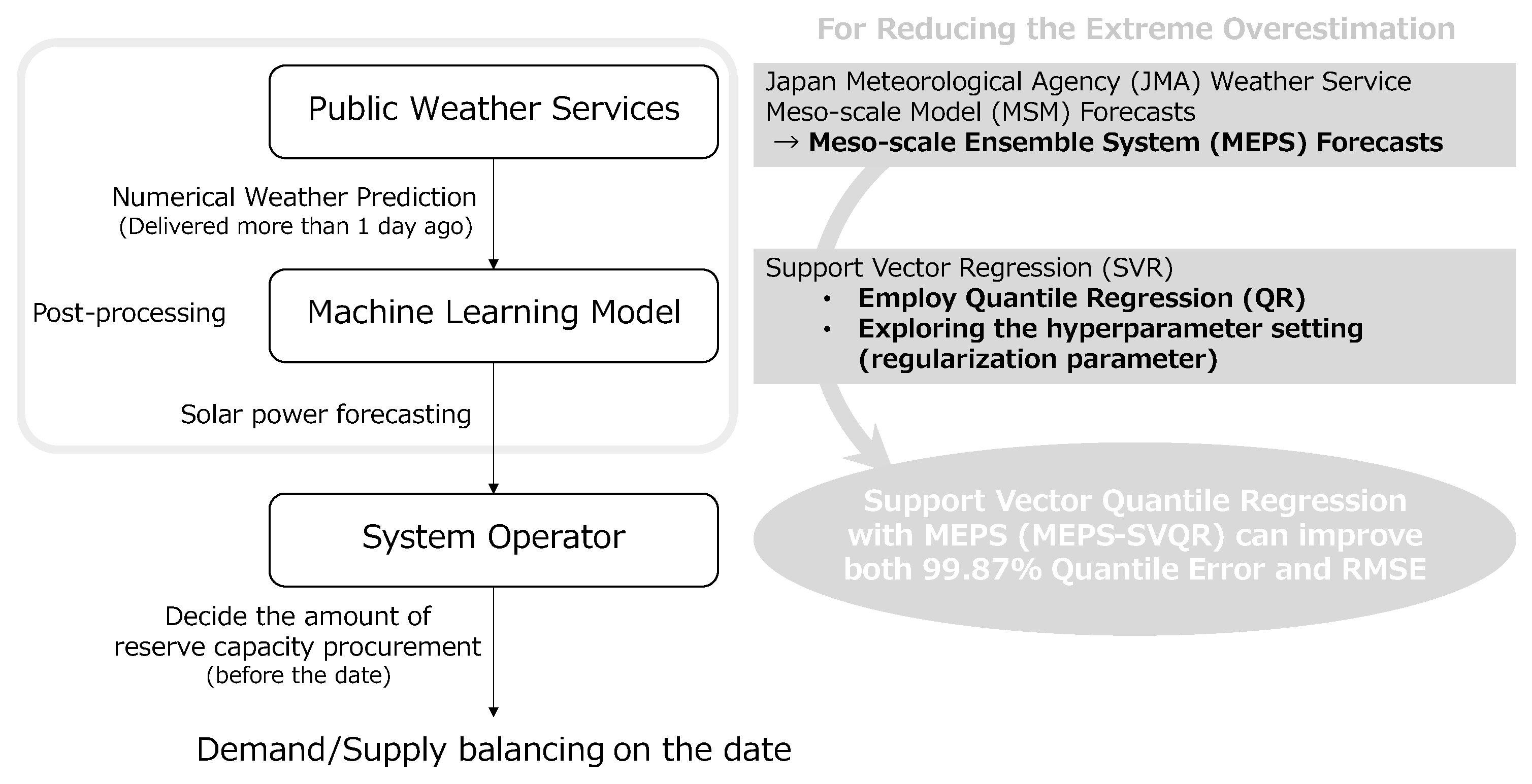
• Adoption of the method for the machine learning model that enables to reduce the overestimation risk;
• Upgrading the NWP data used as explanatory variables;
• Adjustment of hyperparameters.

One of the effective approaches used includes incorporating features to suppress overestimation into the training process of the prediction model. It can be implemented by designing an asymmetric evaluation function that penalizes more heavily for overestimation of solar power. Among the asymmetric evaluation functions, the regression using the asymmetric absolute value loss function (pinball loss function) is called quantile regression (QR), which enables one to estimate different quantiles by varying the slope of the loss function [15]. QR is a useful tool for nonparametric estimation of probability distributions, and it can be combined with simple linear models [16] or machine learning models: Regression trees [17,18], ANN [19,20], or SVR [21,22].

To be noted, although QR is generally used to predict confidence intervals, we assume to use it to tune deterministic forecasts (point forecasts) in this study. This is because there is a feeling for common users that probabilistic forecasts are difficult to manage, and from the viewpoint of usability, deterministic forecasts are more frequently favorably received. QR’s asymmetric weighted penalty is expected to contribute to the regressor reducing the overestimation of point forecasting.

Another risk mitigation approach is to update the NWP data used as input to the machine learning model. Due to the chaotic nature of the atmosphere, the previous day’s forecast of the NWP can deviate significantly due to the exponential growth of errors contained in the initial and boundary conditions [23]. That is, uncertainty in the explanatory variables becomes a problem. To compensate for this uncertainty of the NWP, several countries’ meteorological agencies distribute multiple forecast data by ensemble prediction systems (EPSs); therefore, utilizing multiple forecast data enables us to take into account various weather scenarios that cannot be captured by a single forecast. In other words, machine learning models could cope with various weather situations by EPS data. For example, if one forecast deviates significantly, it is possible to correct the output of the model by referring to other forecasts.

For the regions of Japan, Japan Meteorological Agency (JMA) distributes the EPS forecast for forecasting the meso-scale atmospheric phenomena in Japan and its surrounding area as a Meso-scale Ensemble Prediction System (MEPS), which is based on Meso-scale Model (MSM) forecasts; their multiple forecasts could be utilized for the solar power forecasting of the regions of Japan.

A tertiary approach is to adjust the model parameters. Some parameters need to be specified for the machine learning model, such as the shape of the basis functions and the weights of the regularization terms, and they can be also selected to satisfy certain objectives.

Some researchers have optimized the hyper parameters of their machine learning models by meta-heuristic optimization algorithms: Genetic algorithm (GA) [24], Coral Reefs Optimization (CRO) [25], and Particle Swarm Optimization (PSO) [26,27]. Several review papers regarded them as one class of hybrid models, which is called the Evolutionary based Ensemble Learning Approach (EELA) [28,29].

However, even in those studies, the target of the optimization was the prediction accuracy in a general context (average accuracy), and few research articles give consideration for the purpose of mitigating serious overestimation; the uncertainty of rare events and their impact (risk) is of interest for power system safety.

In spite of the importance of extreme errors in risk management, the relationship between hyperparameters and the prediction models’ worst errors has never been sufficiently examined. On the other hand, in regression problems for noisy data sets, the approach that adjusts the regularization parameters is effective. Thus, it may also have some efficacy in overestimation reduction.

In this study, from the above three approaches, we explore the feasibility of a NWP-based machine learning model design to reduce serious overestimation for solar irradiance forecasts a day-ahead: employing the QR by the SVR model (this paper refers it as support vector quantile regression (SVQR)), adding MEPS data to the explanatory variables and adjusting the regularization parameter. As a numerical experiment, hourly short-term forecasts from the prediction models are tested for surface global horizontal irradiance (GHI) observation on an average of five sites of the JMA stations in the Kanto region in Japan. Serious overestimations are measured by 3$\sigma$ error as metrics and are evaluated together with RMSE through the cross-validation. The results of the numerical simulation tests can be summarized as follows.

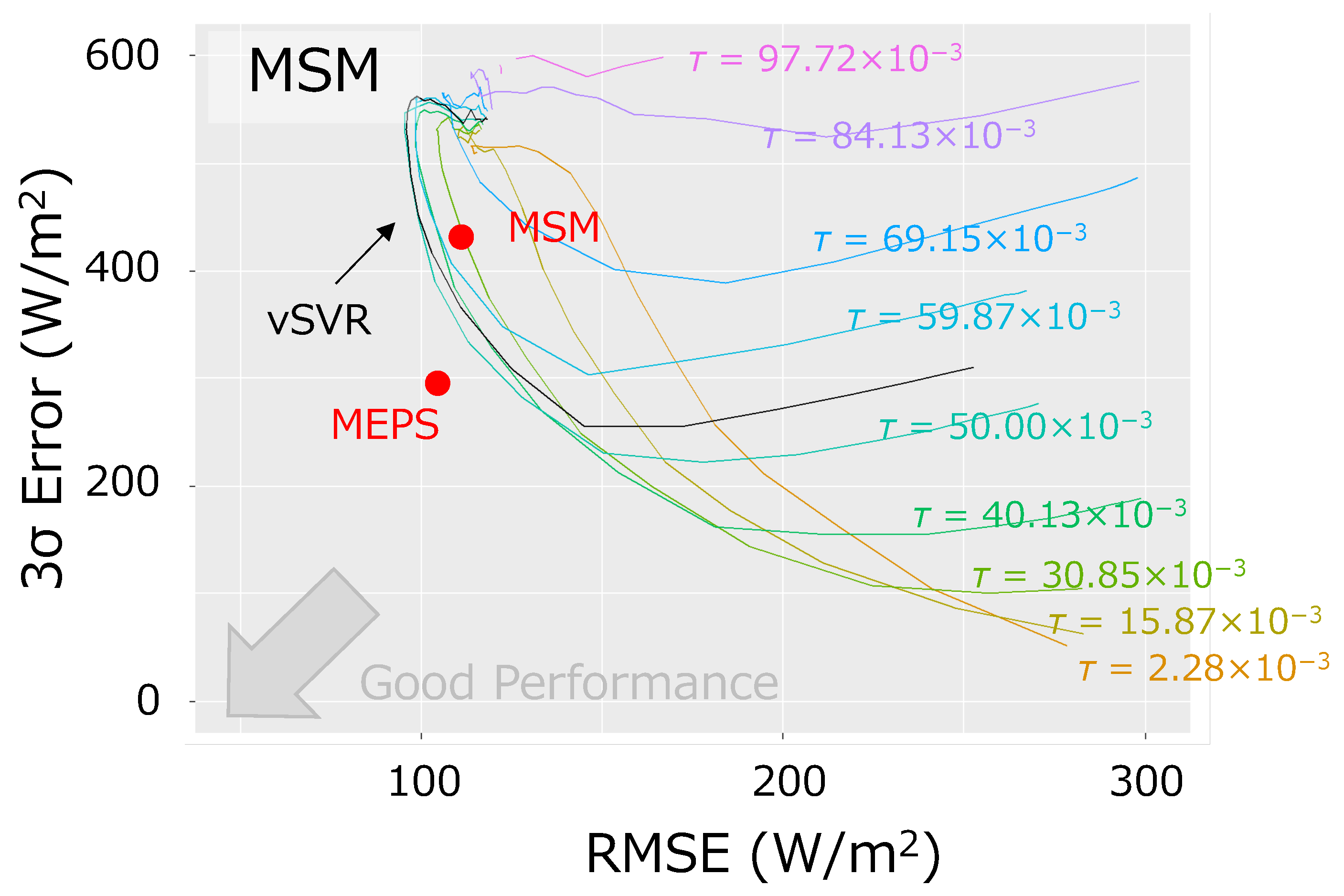
• When the penalty of the regularization term is varied, there tends to be a trade-off between the RMSE of SVR and the 3$\sigma$ error;
• SVR can be used as a post-processing of MEPS data to improve the original data on both metrics;
• Comparing SVQR with the MSM data (MSM-SVQR), SVQR with MEPS data (MEPS-SVQR) is more effective in the 3$\sigma$ error reduction due to quantile regression, and tuning can build a better model for the two metrics.

Among our proposed models, MEPS-SVQR is especially effective in suppressing serious overestimates (3$\sigma$ error), and the use of such a low-risk predictor is expected to help SOs to reduce the procurement of reserve capacity to take measures against extreme forecast errors.

This paper is organized as follows. In Section 2, some approaches regarding the enhancement of numerical weather prediction are described along with recent literature. In Section 3, we denote the description of data. Section 4 explains the fundamental methodology of our study: Support vector regression, quantile regression, metrics for the error assessment, and cross-validation for evaluating our models performance. Section 5 shows the details of our prediction models, and the performance of them is discussed in Section 6. In Section 7, the conclusions are denoted.

Our approach for reducing the extreme overestimation and the summary of this paper are illustrated in Figure 1 and Figure 2.

2. Enhancement of the Numerical Weather Prediction

2.1. Post-Processing Approach Based on Machine Learning

In determining the day-ahead transmission schedule and electricity market operations, short-term solar power forecasting for 1–3 days in advance is used [30]. In such short term solar power forecasting, numerical weather prediction (NWP) is more advantageous than satellite data and cloud imagery forecasting [31]. For the meso-scale atmospheric phenomena in Japanese region, JMA distributes forecasts such as MSM data. However, NWP has limited spatial resolution to grasp the details of clouds, which can lead to errors due to local effects, and systematic errors are sometimes caused by the pre-processing work to obtain a stable numerical solution [32]. In order to suppress these errors, machine learning is recognized as a useful approach for the post-processing tool for NWP [33]. For example, Artificial Neural Network (ANN) [34,35], regression tree [36,37], and Support Vector Regression (SVR) [38,39]. Besides, the recent solar power forecast model research adopts an ensemble learning approach, which integrates multiple models into a hybrid model that enables the predictor to provide more accurate predictions than a conventional single unit [29].

2.2. Stochastic Approach Based on Ensemble Prediction System

Precisely estimated initial and boundary value based forecasting are called deterministic forecasting, and their precision has been enhanced by the progress of observation systems and data assimilation techniques, the refinement of NWP modeling, and the adoption of high-performance computers. However, deterministic approaches are inherently limited in their predictability because the atmosphere has chaotic behavior [23]. To solve this problem, EPS, which combines a deterministic NWP model and probabilistic approach, has been developed. Its multiple forecasts (ensemble members) are generated by making proper perturbations to their base NWP, and the ensemble average of EPS forecasts performs better compared to the original NWP forecast (control member) [40,41].

Operational prediction of EPS was first introduced into global-scale models by the US National Meteorological Center (NMC) in 1992 [42]. Along with the advancement of EPS in global-scale models, researchers have extended EPS to regional-scale models [43]. Until now, prediction systems adopting ensemble forecasts for medium-range models have been in service in many countries. In the U.S., the U.S. National Centers for Environmental Prediction (NCEP) introduced Short Range Ensemble Forecasting (SREF) in 2001 [44], and the UK Meteorological Office (UKMO) introduced the Met Office Global and Regional Ensemble Prediction System (MOGREPS) in 2005 [45]. In 2011, the Meteorological Service of Canada (MSC) launched the Regional Ensemble Prediction System (REPS) [46], and in 2012, the German Meteorological Department (DWD) began operating a regional EPS based on the Council for Small-scale Modeling of the German Regions (COSMO- DE-EPS) started [47]. Prediction systems with ensemble forecasts for mesoscale regional models are in operation in many different countries.

In Japan, JMA started to develop a meso Singular Vector (SV) method in 2005 for Japanese regional-scale EPS. Then, after several comparative experiments, MEPS was introduced in 2015. Operational forecasting for MEPS began in 2019 with the launch of the 10th Generation Numerical Analysis and Prediction System (NAPS10) [48].

Several studies applied the EPS output from European Center for Medium-Range Weather Forecasts (ECMWF) to machine learning models; S. Sperati et al. adopted NN for the post-processing of the ECMWF EPS forecasts for their photovoltaic power forecasting [49], S. Rasp and S. Lerch also employed NN on ECMWF’s EPS forecasts for temperature estimation [50], and L. Massidda and M. Marrocu used QR with Gradient-Boosted Regression Trees (GBRT) to each EPS member and combined their output with Integrated Forecast System (IFS) data [51]. In Japan, the MEPS data, which is based on the MSM data from JMA was used, and several studies were reported, including the study of confidence interval estimation using the Just-in-Time model [52] and the study of post-processing methods for EPS data based on support vector machines [53]. These studies show that EPS data helps to improve the accuracy of PV forecasts. In particular, our recent article [53] suggests that the maximum (minimum) forecast error can be suppressed by the EPS output as an explanatory variable in the SVR.

3. Data Description

3.1. Forecasts of Meso-Ensemble Prediction System

MEPS is a system that generates 20 ensemble members (from 1 control member) by perturbing the initial and lateral boundary conditions of the MSM, and the perturbations are given in meso SV and global SV. MEPS forecasts are given at 00, 06, 12, and 18 UTC, and are capable of forecasting up to 39 h ahead. The MEPS has a spatial resolution of 5 km, and the forecasts of MEPS are hourly previous time averaged data; and furthermore, MEPS is based on the ASUCA model, which is the improved model of the conventional JMA non-hydrostatic model (JMA-NHM) as its dynamical model. (See details in [54]).

Although the GHI forecast provided by MEPS is useful for PV forecasting, MEPS is tuned for preventing heavy rain disaster as the major mission; MEPS is not a product tuned particularly for GHI forecasts’ systematic errors, such as due to cloud microphysical processes and cloud cover calculations of radiative processes.

Similar to the conventional NWP post-processing, the machine learning technique is expected to be useful in correcting the GHI prediction of MEPS. Therefore, the MEPS-based machine learning model can be expected to improve short-term solar irradiance forecasts.

3.2. Surface Observation Data

JMA has meteorological stations in various parts of Japan and collects data from surface observations. These weather stations observe a wide range of data, including temperature, humidity, precipitation, wind direction and speed, snowfall, surface pressure, and solar radiation, and the surface GHI in the Kanto region of Japan has been observed at five sites: Utsunomiya, Maebashi, Tsukuba, Tokyo, and Choshi (their locations are shown in Figure 3). Solar radiation observation data is acquired every second from sunrise to sunset every day by an electric all-sky radiation meter, and quality is checked to meet the requirements of the Baseline Surface Radiation Network (BSRN). (See [55,56] for details). The measured GHI data is converted to previous hourly average data and is distributed from the JMA website [57].

3.3. Performance of the Numerical Weather Prediction

In order to verify the performance of NWP data, it is essential to compare them with the surface observations. Figure 4 shows the correspondence between the one day-ahead forecasts of MSM and MEPS (21-member mean) and ground-based observations for the five-station average GHI from 6 June 2018 to 6 October 2018. In each graph, the upper part of the diagonal line indicates an overestimation and the lower part indicates an underestimation.

MSM and MEPS tend to underestimate, but extreme overestimation occurs when the surface GHI is around 375 (W/m${}^2$) in rare cases; the maximum forecast error reaches 470 (W/m${}^2$) for MSM data and 333 (W/m${}^2$) for MEPS data. Furthermore, the MEPS data has a narrower plot spread from the diagonal compared to the MSM data, which shows that an overall good forecast is obtained by the stochastic approach.

It is also possible to correct the underestimation tendency and improve the accuracy by using a machine learner for post-processing on these forecast data. On the other hand, note that our target is not only to improve the average accuracy, but also to reduce the serious overestimation that rarely occurs.

4. Methodology

4.1. Support Vector Regression

Note that SVR is an implementation of the support vector machines for regression tasks, and K. R. Müller et al. and H. Drucker et al. demonstrated that SVR could achieve good performance in time series forecasting [58,59]. When the standardized dataset is given as $\left({\mathit{x}}^{\left(i\right)},y^{\left(i\right)}\right)i=1,2,\dots ,N$, SVR performs regression with the dataset mapped to a high-dimensional space and constructs the regression equation as a weighted sum of basis functions called kernel functions. If the Radial Basis Function (RBF) is used as the kernel function, the regression equation is constructed as follows:

$$\begin{array}{c}\widehat{f}\left(\mathit{\alpha };\mathit{x}\right)=\sum _i{\alpha }_i{K}_{RBF}\left({\mathit{x}}^{\left(i\right)},\mathit{x}\right),\end{array}$$

(1)

$$\begin{array}{c}{K}_{RBF}\left({\mathit{x}}^{\left(i\right)},\mathit{x}\right)=e^{-\gamma \parallel {\mathit{x}}^{\left(i\right)}{-\mathit{x}\parallel }_2},\end{array}$$

(2)

where the weight parameter $\mathit{\alpha }$ is determined to minimize the evaluation function of the following equation.

$$\begin{array}{c}\underset{\mathit{\xi },\mathit{a},ϵ}{min}\sum _i{\xi }_i+\frac{1}{2}{C}^{-1}{\mathit{\alpha }}^{\mathsf{T}}\mathit{G}\mathit{\alpha }-\nu ϵ,\end{array}$$

(3)

$$\begin{array}{c}\mathit{G}=\left[\begin{array}{cccc}{K}_{RBF}\left({\mathit{x}}^{\left(1\right)},{\mathit{x}}^{\left(1\right)}\right)& K_{RBF}\left({\mathit{x}}^{\left(1\right)},{\mathit{x}}^{\left(2\right)}\right)& \cdots & K_{RBF}\left({\mathit{x}}^{\left(1\right)},{\mathit{x}}^{\left(N\right)}\right)\\ K_{RBF}\left({\mathit{x}}^{\left(2\right)},{\mathit{x}}^{\left(1\right)}\right)& K_{RBF}\left({\mathit{x}}^{\left(2\right)},{\mathit{x}}^{\left(2\right)}\right)& \cdots & K_{RBF}\left({\mathit{x}}^{\left(2\right)},{\mathit{x}}^{\left(N\right)}\right)\\ ⋮& ⋮& \ddots & ⋮\\ K_{RBF}\left({\mathit{x}}^{\left(N\right)},{\mathit{x}}^{\left(1\right)}\right)& K_{RBF}\left({\mathit{x}}^{\left(N\right)},{\mathit{x}}^{\left(2\right)}\right)& \cdots & K_{RBF}\left({\mathit{x}}^{\left(N\right)},{\mathit{x}}^{\left(N\right)}\right)\end{array}\right],\end{array}$$

(4)

$$\begin{array}{c}{\xi }_i=h\left(\widehat{f}\left(\mathit{\alpha };{\mathit{x}}^{\left(i\right)}\right)-y^{\left(i\right)},ϵ\right),\end{array}$$

(5)

$$\begin{array}{c}h\left(e,ϵ\right)=max\left(\left|e\right|-ϵ,0\right),\end{array}$$

(6)

where $h\left(e,ϵ\right)$ is called the hinge loss function, which is a function with an $ϵ$-band that ignores residuals up to $ϵ$, and Figure 5 shows the shape of the function. C and $\nu$ are hyperparameters, where C adjusts the effect of the regularization term and $\nu$ adjusts the width of the hinge loss function’s $ϵ$-insensitive band. The SVR that performs parameter optimization including the width of the $ϵ$-band in the form described above is called $\nu$-SVR, and was proposed by B. Schölkopf et al. in 2000 [60]. A. Smola and B. Schölkopf detailed SVRs’ implementation in [61]. In the environment of the programming language R, the e1071 package [62] is provided as a wrapper for the LibSVM package [63], and it helps R users to implement $\nu$-SVR.

4.2. Quantile Regression

QR is the regression analysis method that estimates the conditional sample quantile from a data set without using the assumption of PDF, whereas ordinary least squares estimates the mean. (see details in [64]).

The regression for the $\tau$ quantile $\left(0\le \tau \le 1\right)$ is formulated in the form of estimating a function by minimizing an asymmetric absolute loss function.

$$\begin{array}{c}{\widehat{f}}_{\tau }=\underset{f\left(\mathit{a};\mathit{x}\right)|\mathit{a}\in A}{arg\; min}\sum _i{\rho }_{\tau }\left(y^{\left(i\right)}-f\left(\mathit{a};{\mathit{x}}^{\left(i\right)}\right)\right),\end{array}$$

(7)

$$\begin{array}{c}{\rho }_{\tau }\left(u\right)=\left\{\begin{array}{cc}\tau u,& u\ge 0\\ \left(\tau -1\right)u,& u<0\end{array}\right.,\end{array}$$

(8)

where $\mathit{a}$ is a parameter of the function and $\mathit{A}$ denotes its set. The asymmetric loss function (pinball loss function) ${\rho }_{\tau }\left(u\right)$ is a function similar to the hinge function $h\left(e,ϵ\right)$ and its shape is shown in Figure 6. Therefore, in the parameter optimization of the SVR represented by Equation (3), it is possible to perform quantile regression with kernel functions using the structure of the SVR by replacing the evaluation of the residuals in Equation () as

$${\xi }_i^{\prime }={\rho }_{\tau }\left(\widehat{f}\left(\mathit{a};{\mathit{x}}^{\left(i\right)}\right)-y^{\left(i\right)}\right).$$

(9)

QR through SVR methodology was reported by Takeuchi et al. in 2004 [65]. It can be used in the R language with packages such as liquidSVM [66] and kernlab [67]. In this study, we employed the liquidSVM package for SVQR implementation.

4.3. Metrics of Error

In the evaluation of prediction models, Mean Bias Error (MBE), Root Mean Square Error (RMSE), and Mean Absolute Error (MAE) are often used as indicators that quantify the residuals between predicted and measured values. (See details in [68]).

Assuming that the measured data and predicted values used for verification are $\left(v^{\left(j\right)},{\widehat{v}}^{\left(j\right)}\right),j=1,2,\dots ,n$, respectively, they can be described by the following equations:

$$\begin{array}{cc}\hfill MBE& =\frac{1}{n}\sum _{j=1}^n\left({\widehat{v}}^{\left(j\right)}-v^{\left(j\right)}\right),\hfill \end{array}$$

(10)

$$\begin{array}{cc}\hfill RMSE& =\sqrt{\frac{1}{n}\sum _{j=1}^n{\left({\widehat{v}}^{\left(j\right)}-v^{\left(j\right)}\right)}^2},\hfill \end{array}$$

(11)

$$\begin{array}{cc}\hfill MAE& =\frac{1}{n}\sum _{j=1}^n\left|{\widehat{v}}^{\left(j\right)}-v^{\left(j\right)}\right|.\hfill \end{array}$$

(12)

When corresponding to the $L_p$ norm, MAE corresponds to the Manhattan distance ($L_1$ norm) and RMSE corresponds to the Euclidean distance ($L_2$ norm) scaled by the number of samples, respectively. The MBE and RMSE are also related to the variance $S{D}^2$ of the statistical distribution of the residuals,

$$S{D}^2=RMS{E}^2-MB{E}^2.$$

(13)

On the other hand, in risk management for rare events, order statistics are often important, rather than average scores, as described above. As an example, there is a reference on the estimation of probable maximum loss using order statistics by Wilkinson [69].

One of the definition of the error quantile can be denoted as the following equations:

$$\begin{array}{c}{E}_q=e_{\left(1-q+qn\right)}0\le q\le 1,\end{array}$$

(14)

$$\begin{array}{c}{e}_{\left(j\right)}=\left\{\begin{array}{cc}min\left\{e_1,e_2,\dots ,e_n\right\}& j=1\hfill \\ min\left\{\left\{e_1,e_2,\dots ,e_n\right\}\setminus \left\{e_{\left(1\right)},e_{\left(2\right)},\dots ,e_{\left(j-1\right)}\right\}\right\}& j=2,3,\dots ,n\hfill \\ \left(\lceil j\rceil -j\right)e_{\left(\lfloor j\rfloor \right)}+\left(j-\lfloor j\rfloor \right)e_{\left(\lceil j\rceil \right)}& j\notin \mathbb{N}\hfill \end{array}\right.,\end{array}$$

(15)

$$\begin{array}{c}{e}_j={\widehat{v}}^{\left(j\right)}-v^{\left(j\right)}j=1,2,\dots ,n,\end{array}$$

(16)

where q is the number of quantile, $e_j$ is a forecasting error, and $e_{\left(j\right)}$ is the j-th order statistic of the errors.

Note that, given the empirical distribution function $F_n\left(e\right)=\frac{1}{n}{\sum }_{j=1}^n{\mathit{1}}_{e_j\le e}$, its q-quantile $F_n^{-1}\left(q\right)=inf\left\{e|F_n\left(e\right)\ge q\right\}$ and the above quantile $E_q$ have the relation $E_q\ge F_n^{-1}\left(q\right)$. By using $E_q$, the overestimation (in case ${\widehat{v}}^{\left(j\right)}-v^{\left(j\right)}>0$) is evaluated to a greater extent than by using $F_n^{-1}\left(q\right)$. In this study, we measure 3$\sigma$ error of the forecasts by $E_q$: it is denoted by $3\sigma \mathrm{error}=E_{q^{\prime }},q^{\prime }={\int }_{-\infty }^{3\sigma }{p}_N\left(z\right)\mathrm{d}z$, where $p_N\left(z\right)$ is the probability density function of the normal distribution $N\left(0,\sigma \right)$. Besides, $E_{q^{\prime }}$ represents the quantile corresponding to 3$\sigma$ in the normal distribution, and is a metrics that does not require the assumption of a probability distribution for the error to be assessed.

4.4. Cross-Validation

For the appropriate performance analysis of the forecasting models, it is essential to properly train and test the predictors in the evaluation process; it is ideal to strictly separate the training data set from the test data set. However, when a dataset with sufficient size is unavailable, the evaluation process could employ k-fold Cross Validation (CV). First, the data is divided into the k folds, second, the models train the data except for the data in the k-th fold, third, the k-th data is applied to assess the score of the model performance, and this process should be repeated until all folds have been applied for the evaluation.

Although CV is a commonly employed tool for assessing model performance, simple division of the date-ordered datasets (without sufficient number of years) could leave seasonal bias between the test and training datasets in each split for the verification. To avoid this, one could prevent both the test and the training data from being unbalanced around some dates.

To evaluate the forecasting results in our work, the 4-fold CV was employed, and random shuffling was performed for each date before the 4-fold CV in order to remove the impact of seasonal trends. In addition, the error data obtained by the CV is evaluated in a lump-sum manner. In the k-fold CV, scores are generally aggregated for each group and the average of the scores is obtained, but we do not separate the groups and treat the results of forecasts for individual samples comprehensively. The configuration of the assessment procedure is shown in Figure 7.

5. Prediction Model

The variables of the dataset are listed in

Table 1. Dataset variables.

Type	Symbol	Description	Source
Objective	$SGH{I}_{\mathrm{avg}}$	Surface GHI on Area Average	JMA stations’ data
Explanatory	$\widehat{EI}$	Extraterrestrial Irradiance	Theoretical form [70]
	$\widehat{T}$	Temperature	MSM
	$\widehat{RH}$	Relative Humidity
	$\widehat{HC}$	High-level Cloud Cover
	$\widehat{MC}$	Middle-level Cloud Cover
	$\widehat{LC}$	Low-level Cloud Cover
	$\widehat{GHI}$	Global Horizontal Irradiance	MSM or MEPS

, where $\widehat{•}$ represents the forecasts or the estimation from theoretical formulas [70]. The data period is four months, from 6 June 2018 to 6 October 2018, and the dataset consists of hourly samples from sunrise to sunset on each day.

$\widehat{EI}$ is a theoretical estimate, calculated from geodetic coordinates and date/time, and $\widehat{T}$, $\widehat{RH}$, $\widehat{HC}$, $\widehat{MC}$, and $\widehat{LC}$ are referred to the MSM forecasts, which is delivered the day before the time t to be forecast (delivered at 15:00 JST). These are variables indexed by the time and an area point for forecasting, and therefore we represent them as $\widehat{•}\left(t;s\right)$, where s is the index number of the area points. On the other hand, the GHI forecasts $\widehat{GHI}$ include the MEPS data, of which the MSM data is a control member. MEPS outputs multiple forecasts based on control members, which means that in addition to the time and area points to be forecast, it has an index indicating the ensemble member as an attribute: we denote MEPS forecasts as $\widehat{GHI}\left(t;s;m\right)$, where m indicates the number of ensemble member, which $m=0$ corresponds to the control member (MSM forecasts). $SGH{I}_{\mathrm{avg}}$ is the objective variable for forecasting, which represents the average surface GHI observation of the five weather stations. In this work, each data is converted to z-scores in standardization as appropriate.

The input–output relationship of prediction models using MEPS data could be represented as follow:

$$\begin{array}{cc}\hfill & {\widehat{SGHI}}_{\mathrm{avg}}\left(t\right)=F\left({\mathit{X}}_t\right),\hfill \\ \hfill {\mathit{X}}_t& =\left[\begin{array}{cccccc}{\widehat{\mathit{EI}}}_t& {\widehat{\mathit{MSM}}}_t& {\widehat{\mathit{GHI}}}_t& {\widehat{\mathit{EI}}}_{t-1}& {\widehat{\mathit{MSM}}}_{t-1}& {\widehat{\mathit{GHI}}}_{t-1}\end{array}\right],\hfill \\ \hfill {\widehat{\mathit{EI}}}_t& =\left[\begin{array}{ccccc}\widehat{EI}\left(t;1\right)& \cdots & \widehat{EI}\left(t;s\right)& \cdots & \widehat{EI}\left(t;n_s\right)\end{array}\right],\hfill \\ \hfill {\widehat{\mathit{MSM}}}_t& =\left[\begin{array}{ccccc}\widehat{\mathit{msm}}\left(t;1\right)& \cdots & \widehat{\mathit{msm}}\left(t;s\right)& \cdots & \widehat{\mathit{msm}}\left(t;n_s\right)\end{array}\right],\hfill \\ \hfill \widehat{\mathit{msm}}\left(t;s\right)& =\left[\begin{array}{ccccc}\widehat{T}\left(t;s\right)& \widehat{RH}\left(t;s\right)& \widehat{HC}\left(t;s\right)& \widehat{MC}\left(t;s\right)& \widehat{LC}\left(t;s\right)\end{array}\right],\hfill \\ \hfill {\widehat{\mathit{GHI}}}_t& =\left[\begin{array}{ccccc}\widehat{\mathit{ghi}}\left(t;0\right)& \cdots & \widehat{\mathit{ghi}}\left(t;m\right)& \cdots & \widehat{\mathit{ghi}}\left(t;n_m\right)\end{array}\right],\hfill \\ \hfill \widehat{\mathit{ghi}}\left(t;m\right)& =\left[\begin{array}{ccccc}\widehat{GHI}\left(t;1;m\right)& \cdots & \widehat{GHI}\left(t;s;m\right)& \cdots & \widehat{GHI}\left(t;n_s;m\right)\end{array}\right],\hfill \end{array}$$

(17)

where ${\widehat{SGHI}}_{\mathrm{avg}}$ is the forecast of $SGH{I}_{\mathrm{avg}}$, $F\left(•\right)$ is a nonlinear function (prediction model) acquired by machine learning, $n_s$ is the number of sites, $n_m$ is the number of ensemble members’ forecasts, and t is the time point to be predicted. Note that, $t-1$ implies the time one step before, which corresponds to one hour before t. In our work, the regression equation corresponding to $F\left(•\right)$ is constructed by MEPS-SVQR and $\nu$-SVR with MEPS (here after MEPS-$\nu$SVR).

In case we only use MSM data, the prediction models could be denoted by

$$\begin{array}{cc}\hfill & {\widehat{SGHI}}_{\mathrm{avg}}^{\prime }\left(t\right)=F^{\prime }\left({\mathit{X}}_t^{\prime }\right),\hfill \\ \hfill {\mathit{X}}_t^{\prime }& =\left[\begin{array}{cccccc}{\widehat{\mathit{EI}}}_t& {\widehat{\mathit{MSM}}}_t& \widehat{\mathit{ghi}}\left(t;0\right)& {\widehat{\mathit{EI}}}_{t-1}& {\widehat{\mathit{MSM}}}_{t-1}& \widehat{\mathit{ghi}}\left(t-1;0\right)\end{array}\right],\hfill \end{array}$$

(18)

where $F^{\prime }\left(•\right)$ is the regression model without the MEPS ensemble members’ forecasts; $\widehat{\mathit{ghi}}\left(t;0\right)$ is equal to the MSM’s GHI forecasts. MSM based prediction models are configured for the comparison with the MEPS based models. We apply MSM data to $\nu$-SVR (MSM-$\nu$SVR) and SVQR (MSM-SVQR).

In each model, the forecasts for one step (one hour) before the time of interest are added as explanatory variables, and the forecasts for the five locations are not summarized, which are used as each separate explanatory variables. Their configuration is shown in Figure 8 and Figure 9. MEPS allows the GHI forecast for each location given by the 20 ensemble members to be added as an explanatory variable. Therefore, compared to a similarly constructed model with only MSM data, our models include 20 members × 5 locations × 2 time steps variables additionally, which is an increase of 200 dimensions in the regression model.

In addition to the description of the model variables, it should be noted that SVQR and $\nu$-SVR each have their own hyperparameters to be set: $\nu$-SVR has a regularization parameter C, $\nu$ which determines the insensitive band width of the hinge loss function, and the decay rate $\gamma$ of the Gaussian kernel. On the other hand, SVQR fixes the hyperparameter of $\nu$-SVR as $\nu =0$ and includes the slope $\tau$ of the asymmetric absolute value loss function as a hyperparameter.

Note that the size of the effect of regularization is related to the suppression of overlearning, and by increasing the effect of regularization, it is possible to construct a model by reducing the effect of noise in the variables. Therefore, in our study, we evaluate the performance of SVR by adjusting the regularization parameter C within a certain range.

We set the hyperparameters as follows: $\nu$ is set as 0.5 (in case SVQR, $\nu =0$), C is set at 35 points in the logarithmic scale range from ${10}^{-3}$ to ${10}^3$, $\gamma$ is set as the inverse of the dimension of the explanatory variables, and $\tau$ is set as ${\Phi }_N\left(z\right),z=\pm 3,\pm 2,\pm 1,\pm 0.5,\pm 0.25,0$, where ${\Phi }_N$ is the CDF of standard normal distribution.

As the numerical simulation for the model verification, the MEPS-$\nu$SVR, MEPS-SVQR, MSM-$\nu$SVR, and MSM-SVQR forecast $SGH{I}_{\mathrm{avg}}$ of five sites in the Kanto region, and their forecasting errors are assessed through the CV process described in Section 4.4. Notably, to ensure that the same CV splits are performed for equitably verification of each model’s performance, regardless of the model difference in the configuration and hyperparameters, the same random seed value was used to shuffle the dates in our work.

6. Results and Discussion

Figure 10 and Figure 11 show the correspondence between the 3$\sigma$ error and RMSE when the regularization parameter C is changed in $\left[{10}^{-3},{10}^3\right]$ for the SVR Models with MEPS or MSM forecasts. Note that the result of the parameter conditions that made the calculation unstable have been removed from the figures. As the RMSE and 3$\sigma$ error, the performance of each model with different regularization parameters can be represented on the coordinates in bidimensional space, respectively. Specifically, the lower left in these binominal spaces represents the better forecasting model in terms of both average accuracy and robustness to the risk of serious overestimation. The results of each model in the lower left curve correspond to the Pareto solution, and the border connecting them continuously corresponds to the Pareto frontier. In the design process of the predictor, the user can set the model configuration and parameters to satisfy the preference solution from the Pareto frontier.

As a trend across all models, when the penalty of the regularization term is large (the C parameter is small), the fitting to the training data becomes inhibitory, resulting in a high RMSE of forecast error while suppressing the overestimation to a low level. Then, as the penalty of the regularization term is reduced (the C parameter is increased), the RMSE decreases and at a certain stage, the 3$\sigma$ error increases. On the other hand, if the C parameter is under-set, an over-fit to the data occurs, causing the RMSE to increase from its bottom value and the 3$\sigma$ error to increase. In addition, it is also confirmed that SVR can improve the input forecast data (MSM or MEPS) in both RMSE and 3$\sigma$ error metrics if the C parameter is properly adjusted. The above suggests that while SVR is useful for improving MSM and MEPS data, to some extent it exhibits a trade-off between RMSE and 3$\sigma$ error in adjusting its regularization parameter. While a regularization parameter of SVR is frequently adjusted with RMSE or MAE, this result implies that a regularization parameter setting could also have a relation with the serious overestimation: the prediction model optimized by RMSE is not necessarily optimal in reducing the $3\sigma$ error.

SVRs with MEPS are generally located in the lower left region than SVRs with MSM; it can be confirmed that the predictor using MEPS tends to be dominant in the both metrics RMSE and 3$\sigma$ error. Besides, in MSM-SVQR, there is no expansion of the Pareto solution regardless of the parameters of the quantile regression in the range of RMSE below 150 (W/m${}^2$), while in MEPS-SVQR, the region of the Pareto solution (Pareto frontier) is expanded depending on the parameters of the quantile regression setting. This can be attributed to the fact that the MEPS forecasts provided various probabilistic situations on solar power incidence as input to the model; moreover, they increased the degree of freedom in the structure of the model. Notably, the Pareto frontier is expanded by MEPS-SVQR in the direction of reducing the 3$\sigma$ error; hence, by the specification of the model parameters, which realize desirable preference solutions, MEPS-SVQR could helps SOs to suppress the amount of reserve capacity procurement.

7. Conclusions

In this paper, the following three approaches are considered for the SVR model to suppress the huge overestimation, which is a serious risk for the power system.

• Use of the QR method to SVR for reducing the risk of forecast errors;
• Increasing the degrees of freedom of the model by adopting MEPS prediction as an explanatory variable;
• Changing the parameters of the regularization parameter C and the pinball-loss function.

The numerical simulation results suggest that the MEPS-SVQR model can be designed as a more optimal model in terms of both RMSE and 3$\sigma$ error compared to the MSM-SVQR model. Extreme errors (especially overestimations) are scarcely taken into account in the design of solar power predictors, even though they have significant implications for power system operation. To the best of our knowledge, this is the first report of a detailed study on a machine learning model that enables robust solar power forecasting that can both achieve average accuracy and suppress overestimation.

However, this study had a limited time period and type of variables for the MEPS data; we will increase both for more valid reporting in future work. While the NWP-based machine learning model has an advantage in predicting the previous day, the uncertainty of the explanatory variables has been a bottleneck. Ensemble members’ forecasts from EPS are useful to compensate for this, and it is hoped that the further development of predictors will combine EPS data and machine learning models in the future. However, the ensemble members of the EPS represent stochastic events, which are variables of a different nature than those forecast by the control members; therefore, it will be important to explore an appropriate method for inputting stochastic information as explanatory variables into the machine learning model for the sophistication of those models.

Note that our study employs the R packages to build the model, which implies that there are fewer barriers to replication in areas where EPS data is delivered. Reducing the risk of huge overestimation is important for both the safety and efficient operation of power systems, and our proposed model would be useful not only for SOs but also for retail electricity suppliers. From the standpoint of social implementation, it becomes important to prepare the tools that allow many users to easily utilize such low-risk predictors in future.

References

1. IEA. Renewables 2020; IEA: Paris, France, 2020; Available online: https://www.iea.org/reports/renewables-2020 (accessed on 14 January 2022).
2. IEA. Renewables 2021; IEA: Paris, France, 2021; Available online: https://www.iea.org/reports/renewables-2021 (accessed on 14 January 2022).
3. ENTSO-E. ENTSO-E Balancing Report 2020. Available online: https://eepublicdownloads.entsoe.eu/clean-documents/Publications/Market%20Committee%20publications/ENTSO-E_Balancing_Report_2020.pdf (accessed on 14 January 2022).
4. Van der Veen, R.A.C. Designing Multinational Electricity Balancing Markets. Ph.D. Thesis, Technische Universiteit Delft, Delft, The Netherlands, 2012. [Google Scholar]
5. Poplavskaya, K.; Lago, J.; De Vries, L. Effect of market design on strategic bidding behavior: Model-based analysis of European electricity balancing markets. Appl. Energy 2020, 270, 115130. [Google Scholar] [CrossRef]
6. Commission Regulation (EU) 2017/1485 of 2 August 2017 Establishing a Guideline on Electricity Transmission System Operation. Available online: https://eur-lex.europa.eu/legal-content/EN/TXT/?uri=CELEX%3A32017R1485 (accessed on 14 January 2022).
7. Elia Transmission Belgium SA/NV, 30 September 2020, Methodology for the Dimensioning of the aFRR Needs. Available online: https://www.elia.be/-/media/project/elia/elia-site/public-consultations/2020/20200930_finalreport_en.pdf (accessed on 14 January 2022).
8. Knorr, K.; Dreher, A.; Böttger, D. Common dimensioning of frequency restoration reserve capacities for european load-frequency control blocks: An advanced dynamic probabilistic approach. Electr. Power Syst. Res. 2019, 170, 358–363. [Google Scholar] [CrossRef]
9. Li, B.; Zhang, J. A review on the integration of probabilistic solar forecasting in power systems. Sol. Energy 2020, 210, 68–86. [Google Scholar] [CrossRef]
10. METI. Cost of Securing Regulating Power to Cope with Errors in Renewable Energy Forecasts; METI: Tokyo, Japan, 2020; Available online: https://www.meti.go.jp/shingikai/enecho/denryoku_gas/saisei_kano/pdf/022_03_00.pdf (accessed on 14 January 2022).
11. IEA. Japan 2021; IEA: Paris, France, 2021; Available online: https://www.iea.org/reports/japan-2021 (accessed on 14 January 2022).
12. Frías-Paredes, L.; Mallor, F.; León, T.; Gastxoxn-Romeo, M. Introducing the Temporal Distortion Index to perform a bidimensional analysis of renewable energy forecast. Energy 2016, 94, 180–194. [Google Scholar] [CrossRef]
13. Vallance, L.; Charbonnier, B.; Paul, N.; Dubost, S.; Blanc, P. Towards a standardized procedure to assess solar forecast accuracy: A new ramp and time alignment metric. Sol. Energy 2017, 150, 408–422. [Google Scholar] [CrossRef]
14. Izidio, D.M.; de Mattos Neto, P.S.; Barbosa, L.; de Oliveira, J.F.; Marinho, M.H.D.N.; Rissi, G.F. Evolutionary Hybrid System for Energy Consumption Forecasting for Smart Meters. Energies 2021, 14, 1794. [Google Scholar] [CrossRef]
15. Koenker, R.; Hallock, K.F. Quantile regression. J. Econ. Perspect. 2001, 15, 143–156. [Google Scholar] [CrossRef]
16. Lauret, P.; David, M.; Pedro, H.T. Probabilistic solar forecasting using quantile regression models. Energies 2017, 10, 1591. [Google Scholar] [CrossRef]
17. Almeida, M.P.; Perpinan, O.; Narvarte, L. PV power forecast using a nonparametric PV model. Sol. Energy 2015, 115, 354–368. [Google Scholar] [CrossRef] [Green Version]
18. Verbois, H.; Rusydi, A.; Thiery, A. Probabilistic forecasting of day-ahead solar irradiance using quantile gradient boosting. Sol. Energy 2018, 173, 313–327. [Google Scholar] [CrossRef]
19. Fernandez-Jimenez, L.A.; Terreros-Olarte, S.; Mendoza-Villena, M.; Garcia-Garrido, E.; Zorzano-Alba, E.; Lara-Santillan, P.M.; Zorzano-Santamaria, P.J.; Falces, A. Day-ahead probabilistic photovoltaic power forecasting models based on quantile regression neural networks. In Proceedings of the 2017 European Conference on Electrical Engineering and Computer Science (EECS), Bern, Switzerland, 17–19 November 2017; pp. 289–294. [Google Scholar]
20. Yu, Y.; Wang, M.; Yan, F.; Yang, M.; Yang, J. Improved convolutional neural network-based quantile regression for regional photovoltaic generation probabilistic forecast. IET Renew. Power Gener. 2020, 14, 2712–2719. [Google Scholar] [CrossRef]
21. He, Y.; Yan, Y.; Xu, Q. Wind and solar power probability density prediction via fuzzy information granulation and support vector quantile regression. Int. J. Electr. Power Energy Syst. 2019, 113, 515–527. [Google Scholar] [CrossRef]
22. Takamatsu, T.; Ohtake, H.; Oozeki, T. Global Horizontal Irradiance Forecast at Kanto Region in Japan by Qunatile Regression of Support Vector Machine. In Proceedings of the 2021 IEEE 48th Photovoltaic Specialists Conference (PVSC), Fort Lauderdale, FL, USA, 20–25 June 2021; pp. 2646–2647. [Google Scholar]
23. Lorenz, E.N. Deterministic nonperiodic flow. J. Atmos. Sci. 1963, 20, 130–141. [Google Scholar] [CrossRef] [Green Version]
24. Aybar-Ruiz, A.; Jiménez-Fernández, S.; Cornejo-Bueno, L.; Casanova-Mateo, C.; Sanz-Justo, J.; Salvador-González, P.; Salcedo-Sanz, S. A novel grouping genetic algorithm–extreme learning machine approach for global solar radiation prediction from numerical weather models inputs. Sol. Energy 2016, 132, 129–142. [Google Scholar] [CrossRef]
25. Salcedo-Sanz, S.; Jiménez-Fernández, S.; Aybar-Ruíz, A.; Casanova-Mateo, C.; Sanz-Justo, J.; García-Herrera, R. A CRO-species optimization scheme for robust global solar radiation statistical downscaling. Renew. Energy 2017, 111, 63–76. [Google Scholar] [CrossRef]
26. Eseye, A.T.; Zhang, J.; Zheng, D. Short-term photovoltaic solar power forecasting using a hybrid Wavelet-PSO-SVM model based on SCADA and Meteorological information. Renew. Energy 2018, 118, 357–367. [Google Scholar] [CrossRef]
27. Ma, Y.; Lv, Q.; Zhang, R.; Zhang, Y.; Zhu, H.; Yin, W. Short-term photovoltaic power forecasting method based on irradiance correction and error forecasting. Energy Rep. 2021, 7, 5495–5509. [Google Scholar] [CrossRef]
28. Yang, B.; Zhu, T.; Cao, P.; Guo, Z.; Zeng, C.; Li, D.; Chen, Y.; Ye, H.; Shao, R.; Shu, H.; et al. Classification and summarization of solar irradiance and power forecasting methods: A thorough review. CSEE J. Power Energy Syst. 2021, 1–19. Available online: https://ieeexplore.ieee.org/document/9535400 (accessed on 10 December 2021). [CrossRef]
29. Guermoui, M.; Melgani, F.; Gairaa, K.; Mekhalfi, M.L. A comprehensive review of hybrid models for solar radiation forecasting. J. Clean. Prod. 2020, 258, 120357. [Google Scholar] [CrossRef]
30. IRENA. Innovation Landscape Brief: Advanced Forecasting of Variable Renewable Power Generation; International Renewable Energy Agency: Abu Dhabi, United Arab Emirates, 2020. [Google Scholar]
31. Browning, K.A.; Collier, C. Nowcasting of precipitation systems. Rev. Geophys. 1989, 27, 345–370. [Google Scholar] [CrossRef]
32. Diagne, M.; David, M.; Lauret, P.; Boland, J.; Schmutz, N. Review of solar irradiance forecasting methods and a proposition for small-scale insular grids. Renew. Sustain. Energy Rev. 2013, 27, 65–76. [Google Scholar] [CrossRef] [Green Version]
33. Haupt, S.E.; Chapman, W.; Adams, S.V.; Kirkwood, C.; Hosking, J.S.; Robinson, N.H.; Lerch, S.; Subramanian, A.C. Towards implementing artificial intelligence post-processing in weather and climate: Proposed actions from the Oxford 2019 workshop. Philos. Trans. R. Soc. A 2021, 379, 20200091. [Google Scholar] [CrossRef] [PubMed]
34. Lauret, P.; Diagne, H.M.; David, M. A neural network post-processing approach to improving NWP solar radiation forecasts. Energy Procedia 2014, 57, 1044–1052. [Google Scholar] [CrossRef]
35. Gari da Silva Fonseca, J., Jr.; Uno, F.; Ohtake, H.; Oozeki, T.; Ogimoto, K. Enhancements in Day-Ahead Forecasts of Solar Irradiation with Machine Learning: A Novel Analysis with the Japanese Mesoscale Model. J. Appl. Meteorol. Climatol. 2020, 59, 1011–1028. [Google Scholar] [CrossRef]
36. Lazorthes, B. A gradient boosting approach for the short term prediction of solarenergy production. In Proceedings of the (AMS 2013–2014 Solar Energy Prediction Contest) 12th Conference on Artificial and Computational Intelligence and Its Applications to the Environmental Sciences, Atlanta, GA, USA, 2–6 February 2014; Available online: https://ams.confex.com/ams/94Annual/webprogram/Session3537 (accessed on 14 January 2022).
37. Torres-Barrán, A.; Alonso, Á.; Dorronsoro, J.R. Regression tree ensembles for wind energy and solar radiation prediction. Neurocomputing 2017, 326, 151–160. [Google Scholar] [CrossRef]
38. Gari da Silva Fonseca, J., Jr.; Oozeki, T.; Ohtake, H.; Shimose, K.; Takashima, T.; Ogimoto, K. Analysis of different techniques to set support vector regression to forecast insolation in Tsukuba, Japan. J. Int. Counc. Electr. Eng. 2013, 3, 121–128. [Google Scholar] [CrossRef]
39. Gala, Y.; Fernández, Á.; Díaz, J.; Dorronsoro, J.R. Support vector forecasting of solar radiation values. In Proceedings of the International Conference on Hybrid Artificial Intelligence Systems, Salamanca, Spain, 11–13 September 2013; Springer: Berlin/Heidelberg, Germnay, 2013. [Google Scholar]
40. Epstein, E.S. Stochastic dynamic prediction. Tellus 1969, 21, 739–759. [Google Scholar] [CrossRef]
41. Leith, C.E. Theoretical skill of Monte Carlo forecasts. Mon. Weather Rev. 1974, 102, 409–418. [Google Scholar] [CrossRef] [Green Version]
42. Toth, Z.; Kalnay, E. Ensemble forecasting at NMC: The generation of perturbations. Bull. Am. Meteorol. Soc. 1993, 74, 2317–2330. [Google Scholar] [CrossRef] [Green Version]
43. Hou, D.; Kalnay, E.; Droegemeier, K.K. Objective verification of the SAMEX’98 ensemble forecasts. Mon. Weather Rev. 2001, 129, 73–91. [Google Scholar] [CrossRef]
44. Du, J.; Tracton, M.S. Implementation of a Real-Time Short Range Ensemble Forecasting System at NCEP: An update. In Proceedings of the 9th Conference on Mesoscale Processes, Fort Lauderdale, FL, USA, 29 July–2 August 2001. [Google Scholar]
45. Bowler, N.E.; Arribas, A.; Mylne, K.; Robertson, K.B.R.; Beare, S.E. The MOGREPS short-range ensemble prediction system. Q. J. R. Meteorol. Soc. J. Atmos. Sci. Appl. Meteorol. Phys. Oceanogr. 2008, 134, 703–722. [Google Scholar] [CrossRef]
46. Erfani, A.; Frenette, R.; Gagnon, N.; Charron, M.; Beauregaurd, S.; Giguère, A.; Parent, A. The New Regional Ensemble Prediction System at 15 km Horizontal Grid Spacing (REPS 2.0.1), Canadian Meteorological Centre Technical Note. Available online: https://collaboration.cmc.ec.gc.ca/cmc/cmoi/product_guide/docs/lib/technote_reps201_20131204_e.pdf (accessed on 14 January 2022).
47. Gebhardt, C.; Theis, S.E.; Paulat, M.; Bouallègue, Z.B. Uncertainties in COSMO-DE precipitation forecasts introduced by model perturbations and variation of lateral boundaries. Atmos. Res. 2011, 100, 168–177. [Google Scholar] [CrossRef]
48. Ono, K.; Kunii, M.; Honda, Y. The regional model-based Mesoscale Ensemble Prediction System, MEPS, at the Japan Meteorological Agency. Q. J. R. Meteorol. Soc. 2021, 147, 465–484. [Google Scholar] [CrossRef]
49. Sperati, S.; Alessandrini, S.; Delle Monache, L. An application of the ECMWF Ensemble Prediction System for short-term solar power forecasting. Sol. Energy 2016, 133, 437–450. [Google Scholar] [CrossRef] [Green Version]
50. Rasp, S.; Lerch, S. Neural networks for postprocessing ensemble weather forecasts. Mon. Weather. Rev. 2018, 146, 3885–3900. [Google Scholar] [CrossRef] [Green Version]
51. Massidda, L.; Marrocu, M. Quantile regression post-processing of weather forecast for short-term solar power probabilistic forecasting. Energies 2018, 11, 1763. [Google Scholar] [CrossRef] [Green Version]
52. Mori, Y.; Wakao, S.; Ohtake, H.; Oozeki, T.; Takamatsu, T.; Nakaegawa, T.; Honda, Y. Fundamental Study on Interval Estimation of Solar Irradiance by Just-In-Time Modeling with MEPS. In Proceedings of the 2020 Annual Conference of Power and Energy Society, Online Meeting, 2–6 August 2020; Available online: https://www.bookpark.ne.jp/cm/ieej/detail/IEEJ-BTB2020176-PDF/ (accessed on 15 December 2021).
53. Takamatsu, T.; Ohtake, H.; Oozeki, T.; Nakaegawa, T.; Honda, Y.; Kazumori, M. Regional Solar Irradiance Forecast for Kanto Region by Support Vector Regression Using Forecast of Meso-Ensemble Prediction System. Energies 2020, 14, 3245. [Google Scholar] [CrossRef]
54. Japan Meteorological Agency. Numerical Weather Prediction Activities. Available online: https://www.jma.go.jp/jma/en/Activities/nwp.html (accessed on 14 January 2022).
55. Japan Meteorological Agency. Surface Observation. Available online: https://www.jma.go.jp/jma/en/Activities/surf/surf.html (accessed on 14 January 2022).
56. Japan Meteorological Agency. Observation of Solar Radiation. Available online: https://www.jma-net.go.jp/kousou/obs_third_div/rad/rad_sol-e.html (accessed on 14 January 2022).
57. Japan Meteorological Agency. Past Weather Data Download. Available online: http://www.data.jma.go.jp/gmd/risk/obsdl/index.php (accessed on 14 January 2022).
58. Müller, K.R.; Smola, A.J.; Rätsch, G.; Schölkopf, B.; Kohlmorgen, J.; Vapnik, V. Predicting time series with support vector machines. In Proceedings of the 7th International Conference, Lausanne, Switzerland, 8–10 October 1997. [Google Scholar]
59. Drucker, H.; Burges, C.J.; Kaufman, L.; Smola, A.; Vapnik, V. Support vector regression machines. Adv. Neural Inf. Process. Syst. 1997, 9, 155–161. [Google Scholar]
60. Schölkopf, B.; Smola, A.J.; Williamson, R.C.; Bartlett, P.L. New support vector algorithms. Neural Comput. 2000, 12, 1207–1245. [Google Scholar] [CrossRef]
61. Smola, A.J.; Schölkopf, B. A tutorial on support vector regression. Stat. Comput. 2004, 14, 199–222. [Google Scholar] [CrossRef] [Green Version]
62. Meyer, D.; Dimitriadou, E.; Hornik, K.; Weingessel, A.; Leisch, F. e1071: Misc Functions of the Department of Statistics, Probability Theory Group (Formerly: E1071). TUWien. R Package Version 1.7-4. 2020. Available online: https://CRAN.R-project.org/package=e1071 (accessed on 14 January 2022).
63. Chang, C.C.; Lin, C.J. LIBSVM: A library for support vector machines. ACM Trans. Intell. Syst. Technol. (TIST) 2011, 2, 1–27. [Google Scholar] [CrossRef]
64. Koenker, R. Quantile Regression; Econometric Society Monographs; Cambridge University Press: Cambridge, UK, 2005. [Google Scholar]
65. Takeuchi, I.; Furuhashi, T. Non-crossing quantile regressions by SVM. In Proceedings of the 2004 IEEE International Joint Conference on Neural Networks, Budapest, Hungary, 25–29 July 2004; Volume 1, pp. 401–406. [Google Scholar]
66. Steinwart, I.; Thomann, P. liquidSVM: A Fast and Versatile SVM Package. arXiv 2017, arXiv:1702.06899. [Google Scholar]
67. Karatzoglou, A.; Smola, A.; Hornik, K.; Zeileis, A. kernlab—An S4 Package for Kernel Methods in R. J. Stat. Softw. 2004, 11, 1–20. [Google Scholar] [CrossRef] [Green Version]
68. Yang, D.; Alessandrini, S.; Antonanzas, J.; Antonanzas-Torres, F.; Badescu, V.; Beyer, H.G.; Blaga, R.; Boland, J.; Bright, J.M.; Coimbra, C.F.; et al. Verification of deterministic solar forecasts. Sol. Energy 2020, 210, 20–37. [Google Scholar] [CrossRef]
69. Wilkinson, M.E. Estimating Probable Maximum Loss with Order Statistics. Casualty Actuarial Society Forum. 1982, pp. 195–209. Available online: https://citeseerx.ist.psu.edu/viewdoc/download?doi=10.1.1.491.3144&rep=rep1&type=pdf (accessed on 15 January 2022).
70. Liou, K.N. An Introduction to Atmospheric Radiation, 2nd ed.; Academic Press: London, UK, 2002; Available online: https://www.elsevier.com/books/an-introduction-to-atmospheric-radiation/liou/978-0-12-451451-5 (accessed on 15 January 2022).
Figure 1. The flow of the short-term solar power forecasting and the correspondence to this paper’s approach.
Energies 15 01330 g001
Figure 2. Summary of this paper. The white text indicates the parts that are closely related to our work for reducing extreme overestimation.
Energies 15 01330 g002
Figure 3. Location of the JMA station which acquires surface GHI observation in the Kanto region.
Energies 15 01330 g003
Figure 4. Forecast of average GHI at five sites in the Kanto region by MSM and MEPS. MEPS data is represented by the average of the 21 member forecasts.
Energies 15 01330 g004
Figure 5. Hinge loss function.
Energies 15 01330 g005
Figure 6. Pinball loss function.
Energies 15 01330 g006
Figure 7. Structure FL of the evaluation process. Shuffle the dataset FL by the date before the CV process FL, and finally aggregate the FL prediction results together FL.
Energies 15 01330 g007
Figure 8. Configuration of SVR models with MEPS forecasts.
Energies 15 01330 g008
Figure 9. Configuration of SVR models with MSM forecasts. Note that the control member forecasts of MEPS is equal to MSM forecasts.
Energies 15 01330 g009
Figure 10. RMSE vs. 3 σ error for the MEPS- ν SVR and MEPS-SVQR.
Energies 15 01330 g010
Figure 11. RMSE vs. 3 σ error for the MSM- ν SVR and MSM-SVQR.
Energies 15 01330 g011