
A Review on the Unit Commitment Problem: Approaches, Techniques, and Resolution Methods


Abstract
:1. Introduction
- Production cost: This cost is related to the fuel consumption of the thermal units when electricity is generated. Its behavior is usually described through a linear or quadratic function, where there are a fixed term, a linear term concerning the power production, and a quadratic term that multiplies the squared power generation of the unit. The last term can be omitted to work with linear objective functions. Moreover, a piecewise approximation can also be used to linearize the quadratic function. The utilization of integer variables is mandatory for correctly modeling this cost.
- Start-up (SU) cost: This cost is related to the fuel consumption of the starting-up process before a thermal unit is totally committed. It has an exponential behavior according to the number of hours that the unit had been offline. Nevertheless, it is commonly linearized through a stairwise function. Integer variables are also employed for achieving an accurate representation.
- Shut-down (SD) cost: This cost is applied when a thermal unit is shut-down. It is usually modeled as a fixed cost where integer variables are used to define its treatment. Sometimes, this cost is not considered.
- Emission cost: This cost is related to the polluting compounds or the greenhouse gases generated as a consequence of electricity production. It is not linked to the fuel prices, such as those mentioned above, but it is related to fuel consumption and technological efficiency. Its value depends on the local regulation and the emission allowance trading market scheme if it exists. Within the European Union, it relies on CO prices.
- Maintenance cost: This cost represents the increase of the maintenance operations when the thermal unit is running for a longer time. It is modeled as a linear function with respect to power generation, and it is often internalized in the production cost for the sake of simplicity. Integer variables are also associated with this cost.
- Demand constraint: This is a balance equation to assure that the electricity generation meets the load demand for every represented time period. An energy storage term can be added if more accurate management is desired. In turn, it is also possible to introduce a spillage term in the equation to represent situations of production surpluses. It is a linear equation with continuous variables.
- Reserve constraint: This inequality guarantees a technical necessity of power systems, which is the availability of an extra generation capacity reserved for compromising situations, such as a failure in a committed thermal unit, to keep the security of supply. It is a linear inequality that also employs continuous variables.
- Capacity limits: This inequality is used to assure that the electricity generation of each thermal unit respects the minimum and maximum power output according to their technical limits. This inequality is linear and uses integer variables.
- Ramping limits: This inequality assures that the difference between the power generation of a thermal unit during the previous and the current time step does not exceed the ramping rates. It is a linear inequality that uses continuous variables.
- Logic constraint: It establishes logic in the commitment decisions at every time step, indicating the relationships between start-ups, shut-downs, and commitment status along the whole time span. This equation is linear and utilizes integer variables.
- Minimum time up (TU) and time down (TD): This inequality is used to guarantee that the unit is online for a minimum period of time since it is started-up or that it is offline for a minimum time since it is shut-down, in order to accomplish with technical limitations that reduce the risk of failure. It is linear and employs integer variables.
- Operating constraints: This group gathers the constraints that are utilized for a more accurate representation of the operation of the thermal units from a technical point of view. Some examples are situations where some units must run or have a fixed power output, an outage of a unit due to maintenance tasks, or unforeseen problems, etc.
- Emission constraints: They are imposed to bound specific emissions along a time span.
- Network constraints: These constraints are implemented with the aim of representing technical limitations regarding the consideration of the power grid. They increase the accuracy of the unit commitment problem but also the complexity of its resolution. For that reason, the network is frequently disregarded unless a more secure generation schedule is desired. In that case, the capacity of the optimal schedule to overcome an unexpected failure safely is sought. It is known as the Security Constrained Unit Commitment problem (SCUC).
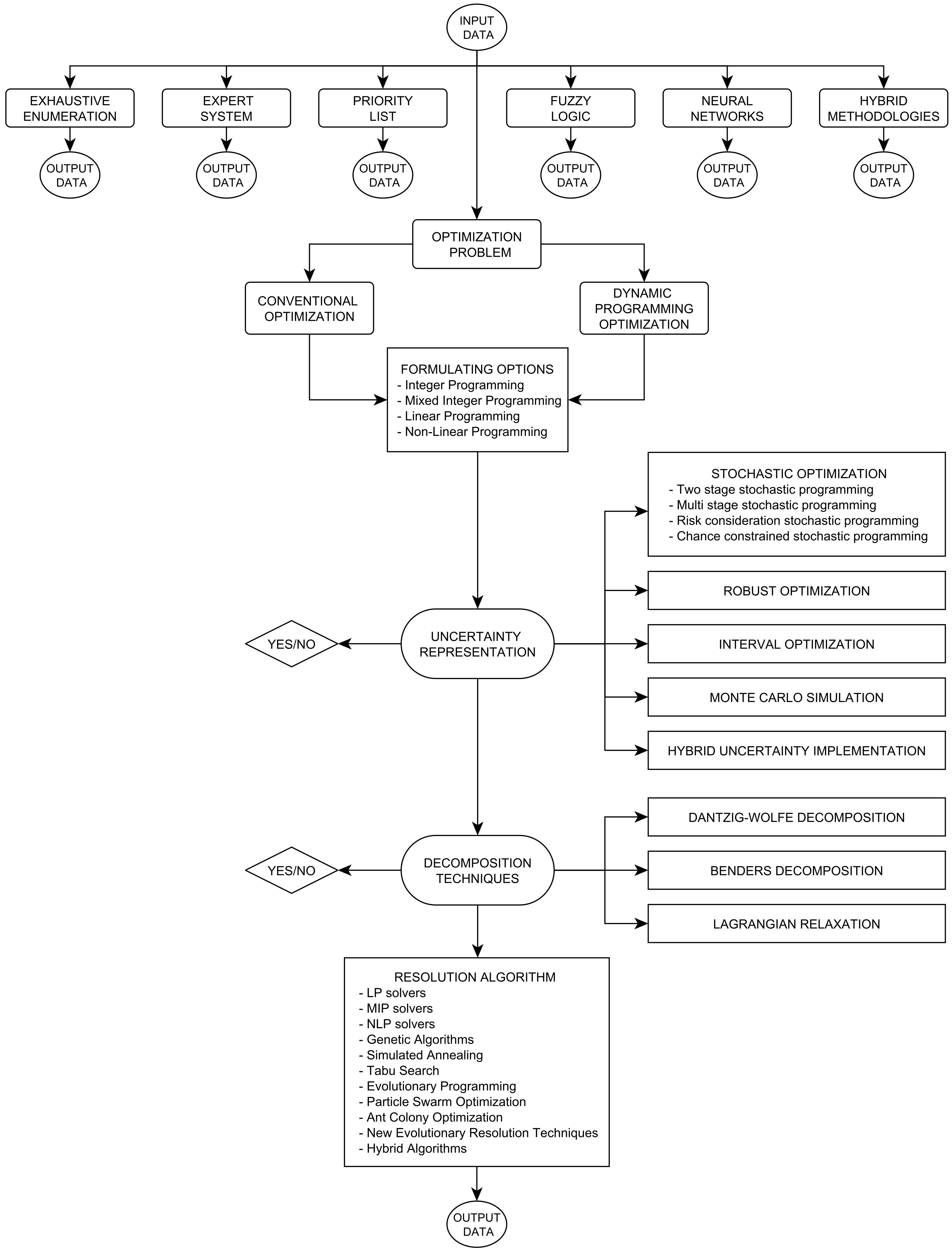
2. Optimization Techniques and Unit Commitment
- Exhaustive Enumeration (EE): It consists of the evaluation of all the feasible solutions in order to identify the best value as the optimal solution. Exhaustive enumeration is a brute force method that is not computationally affordable. Its scope is very limited [2].
- Expert System (ES): The underlying idea of this method resides in the creation of an algorithm where the good practices and knowledge of proceedings in the resolution of the unit commitment problem are computed. It was employed to save in computational costs [3], but it fell into disuse because of its sub-optimal solutions.
- Priority List (PL): This technique is based on ordering elements of target sets according to their contribution to the objective function. The decisions taken on these target elements during the resolution process will conclude in a better or worse approach to the optimal solution. For that reason, it usually has a mathematical background behind it. Despite returning a sub-optimal solution, it is an attractive optimization technique from a computational perspective due to the obtaining of near-optimal solutions in reasonable run times [4,5,6,7].
- Fuzzy Logic (FL): This method allows the application of abstract reasoning into the computational logic to solve a mathematical problem. It utilizes if–then rules in order to generalize some input data. This information is treated according to a background (if conditions) and output data are obtained consequently (then reactions). The utilization of fuzzy logic techniques helps accelerate the resolution of the unit commitment problems but returns a less accurate solution. They are usually applied at a beginning step and combined with other optimization techniques in hybrid proceedings [8,9,10].
- Neural Networks (NN): This artificial intelligence technique is based on establishing patterns that transform some input data into a near-optimal solution. Its structure consists of a group of interconnected nodes where some mathematical functions are applied to process the information. In order to achieve good results, these processes are trained with a benchmark database. However, it provides sub-optimal solutions, and its implementation and adjustment are quite difficult [11,12]. This machine-learning approach is still being used to solve the unit commitment problem nowadays. For further information about the application of machine learning techniques in the unit commitment, the reader is referred to [13].
- Optimization Problem (OP): The unit commitment problem is frequently addressed as a classical optimization problem, where an objective function is proposed, subject to a set of constraints. This methodology entails the most widespread approach used to solve the unit commitment problem, and it is described in depth in Section 3.
3. Unit Commitment as an Optimization Problem
3.1. Formulating Options
3.2. Uncertainty Representation
- Stochastic Optimization (SO): This methodology manages the representation of uncertainty through the utilization of probability distributions that are connected to risk variables. These distributions can be directly included in constraints that require some statistical parameters. Nonetheless, the most common practice is to consider different scenarios. These scenarios are obtained through probability-distribution discretizations. Each scenario has an associated weight according to its frequency of occurrence.
- -
- Two-Stage (TS) Stochastic Programming: This technique is based on dividing the problem into two steps, distributing decision variables and constraints in these stages. When the first step is accomplished, the first-stage choices are made. Later, these decisions are considered fixed, and the second stage is solved. The two-stage stochastic programming utilizes scenarios to consider uncertainty. When all the scenarios are solved, a solution to the problem is calculated according to the weight of each scenario. It has been widely applied in the UC literature [31,32,33,34,35,36,37,38,39]. It is widespread to decide which thermal units will be online along the time span in the first stage. Thereafter, the optimal schedule is set in the second stage. Each dispatch obtained in this stage corresponds to a scenario.
- -
- Multi-Stage (MS) Stochastic Programming: This technique uses a combinatorial tree where every combination of scenarios is represented. The tree is divided into successive nodes that are linked. A branch represents the path between the initial node and a final solution. The weights of scenarios are set in the linking connection between nodes. Thus, it is easy to determine the probability of each solution obtained when each branch is solved, which corresponds to a scenario. Some of its applications to the unit commitment problem are [40,41,42]. Robust solutions are provided, since decisions are taken dynamically. However, the associated computational burden requires an excellent scenario sampling and reduction to reach acceptable run times.
- -
- Risk Consideration (RC) Stochastic Programming: This method is based on the addition of some constraints in order to respect the risk exposure of some decisions when the problem is solved. These equations require statistical information of the probability distributions as input and the significant value desired to respect. Thus, a solution is obtained according to the confidence interval that is introduced in the problem. This technique has been applied to the unit commitment problem in order to represent situations such as the expected non served load, loss of load probability, or the variance of the total profit [43,44,45].
- -
- Chance Constrained (CCO) Stochastic Programming: It is considered a particularization of two-stage stochastic programming. This technique allows the solution to violate a set of constraints according to a predefined confidence level. As with the risk consideration stochastic programming, it works with probability distributions instead of scenarios. However, the solution has a probabilistic touch. It will be the optimal solution with a confidence interval, not according to a confidence interval associated with risk variables [46,47,48].
- Robust Optimization (RO): The underlying idea of this methodology is to reach an optimal solution avoiding the worst possible combination of circumstances that can happen according to the uncertainty associated with the presence of risk variables. Robust optimization does not work with probability distributions. It employs a bounded range from which a risk variable can take its value. The bounds imposed on the risk variables are applied in two ways. They are directly used as upper and lower bounds in an inequality that is defined for each dimension in which the variables are formulated and indirectly through the establishment of an uncertainty set. This uncertainty budget is linked to the deviation of the forecasted value associated with each risk variable from their bounds along the evaluated horizon. It can not exceed a predefined value. The more restrictive the uncertainty set is, the more robust the obtained solution. The load demand is used as the target of RO in the unit commitment problem [49,50,51].
- Interval Optimization (IO): This technique handles the uncertainty representation through the creation of bounds according to a predefined confidence interval. Firstly, a forecasted value is provided for each considered risk variable. Later, the confidence interval is used to generate an envelope around the expected value. The higher the value of the confidence interval, the tighter the bounding to the risk variable. Afterwards, the problem is optimized at the expected central value of the interval, being also capable of providing a feasible solution for those deviations from the forecast that are contained inside the interval [52,53,54].
- Monte Carlo Simulation (MCS): The Monte Carlo methodology is frequently employed to achieve an accurate sampling from a set of probabilistic distributions. However, it can be extended to manage a complete uncertainty representation. In that case, the obtained scenarios are optimized as deterministic problems. Later, the output data are processed, and a probabilistic distribution is associated with each result [55,56,57].
3.3. Decomposition Techniques
3.4. Optimization Algorithms
- Genetic Algorithm (GA): [68].
- Simulated Annealing (SA): [69].
- Tabu Search Algorithm (TSA): [70].
- Evolutionary Programming (EP): [71].
- Particle Swarm Optimization (PSO): [72].
- Ant Colony Optimization (ACO): [73].
- Ant Lion Optimizer (ALO): [74].
- Artificial Bee Colony Algorithm (ABCA): [75].
- Artificial Fish Swarm Algorithm (AFSA): [76].
- Artificial Immune System Algorithm (AISA): [77].
- Artificial Sheep Algorithm (ASA): [78].
- Bacterial Foraging Algorithm (BFA): [79].
- Cuckoo Search Algorithm (CSA): [80].
- Differential Evolution Algorithm (DEA): [81].
- Exchange Market Algorithm (EMA): [82].
- Firefly Algorithm (FFA): [83].
- Fireworks Algorithm (FWA): [84].
- Gravitational Search Algorithm (GSA): [85].
- Grey Wolf Optimizer (GWO): [86].
- Imperialist Competitive Algorithm (ICA): [87].
- Intensify Harris Hawks Optimizer (IHHO): [88].
- Memory Management Algorithm (MMA): [89].
- Quantum-Inspired Evolutionary Algorithm (QIEA): [90].
- Quasi-Oppositional Teaching Learning Based Algorithm (QOTLBA): [91].
- Shuffled Frog Leaping Algorithm (SFLA): [92].
- Sine–Cosine Algorithm (SCA): [93].
- Whale Optimization Algorithm (WOA): [94].
4. Trends in Computational Efficiency to Solve the Unit Commitment Problem
4.1. Evolution of Unit Commitment Modeling Trends and Current Situation
4.2. Precise Description of the Modeling Detail Adopted in the Literature
- The number of segments in piecewise linearizations is specified when they are reported. If they are not given in the table, it means that quadratic coefficients were presented in the paper, and the author just said that the function was linearized.
- Hourly granularity is considered unless another specification is shown in the time span column. Additionally, time period chronology is also supposed to be respected except if a disaggregation technique is mentioned in that column.
- The symbol (r) means replication. It is shown when the number of units that compose a generation portfolio is repeated to deal with bigger systems in the case study or when the data presented for a shorter time span (typically a day) are imitated to make it longer. It entails computational conditions such as symmetry or identifiable patterns.
- The information presented in the demand constraint column denotes the elements that participate in the balance equation. If it is described as equal or greater, the unit commitment problem is addressed as a cost minimization problem where the load demand has to be matched or exceeded, respectively. In the case of PBUC, it is assumed that the maximization has no generation limits unless a (lower) term is added to show that total generation must not exceed the load demand.
- The information presented in the reserve constraints column is not always consistent. Some systems include spinning reserve in primary, secondary, or tertiary reserves. However, other systems establish different distinctions. The reserve dependence on the regulatory framework is out of the scope of this review. For that reason, reserves are shown as they are specified in each paper.
- The operative constraints column is sometimes used to show miscellaneous information, such as hydro representation, market specifications, etc., for the sake of clarity. Thus, the whole case study information is presented in the same row and table, despite space limitations.
- The optimal column determines the capability of the proposed methodology to assure finding the global optimum. In turn, when the paper reports the value of the relative optimality criterion, which is imposed on MIP solvers, it is also exposed in this column. This optimality gap is the quotient of the difference between primal and dual bound, in absolute value, and the maximum of both. This feature can be specified before solving an MIP problem. It should not be confused with the dual gap (defined when decomposition techniques are applied) or the integrality gap (calculated when the optimization ends). It clarifies the scope of the methodologies, providing a significant idea about their efficiency and the trade-off between modeling detail, run time, and computational performance.
- Executions are made in regular computing machines up to the date of the publications to whom any researcher could have access. If they are run in high efficient clusters, whose affordability is limited to generation companies or universities, it will be specified in the run time column.
- The data used in each case study are supposed to be given or properly cited. If some technical or economic aspect is modeled, but any input data are provided, it is specified with a (*). Moreover, if these data are apparently given, but the link is offline by the date that this review is sent to the publisher or the referenced article does not provide the information, it is specified with a (**).
- The generation limits of the thermal units are always considered to be given, except if the rest of the information is also missing.
- If there is at least one start-up cost represented in the methodology, the logic constraint that establishes commitments, start-ups, and shut-downs is formulated.
5. Conclusions
Author Contributions
Funding
Institutional Review Board Statement
Informed Consent Statement
Conflicts of Interest
Abbreviations
| ACO | Ant Colony Optimization |
| AGC | Automatic Generation Control |
| ALO | Ant Lion Optimizer |
| ABCA | Artificial Bee Colony Algorithm |
| AFSA | Artificial Fish Swarm Algorithm |
| AISA | Artificial Immune System Algorithm |
| ASA | Artificial Sheep Algorithm |
| BD | Benders Decomposition |
| BFA | Bacterial Foraging Algorithm |
| CAES | Compressed Air Energy Storage |
| CCGT | Combined Cycle Gas Turbine |
| CO | Conventional Optimization |
| CCO | Chance Constrained Optimization |
| CSA | Cuckoo Search Algorithm |
| DEA | Differential Evolution Algorithm |
| DS | Distribution System |
| DSO | Distribution System Operator |
| DP | Dynamic Programming |
| DWD | Dantzig-Wolfe Decomposition |
| EA | Electrolytic Aluminium series |
| EE | Exhaustive Enumeration |
| EF | Electrolytic arc Furnance |
| EIE | Energy Intensive Enterprise |
| EMA | Exchange Market Algorithm |
| EO | Evolutionary Optimization |
| EP | Evolutionary Programming |
| ES | Expert System |
| ESS | Energy Storage System |
| EV | Electric Vehicle |
| FBU | Fuel Blending Unit |
| FFA | Firefly Algorithm |
| FL | Fuzzy Logic |
| FSU | Fuel Switching Unit |
| FWA | Fireworks Algorithm |
| GA | Genetic Algorithm |
| GSA | Gravitational Search Algorithm |
| GWO | Grey Wolf Optimizer |
| HCCP | Hybrid Combined Cycle Plants |
| HM | Hybrid Methodologies |
| HS | Hydro Spillage |
| HR | Head Range |
| HUI | Hybrid Uncertainty Implementation |
| ICA | Imperialist Competitive Algorithm |
| IHHO | Intensify Harris Hawks Optimizer |
| IO | Interval Optimization |
| IP | Integer Programming |
| IPP | Independent Power Producer |
| LNG | Liquefied Natural Gas |
| LP | Linear Programming |
| LR | Lagrangian Relaxation |
| MCS | Monte Carlo Simulation |
| MILP | Mixed Integer Linear Programming |
| MIQP | Mixed Integer Quadratic Programming |
| MIQCP | Mixed Integer Quadratically Constrained Programming |
| MINLP | Mixed Integer Non Linear Programming |
| MIP | Mixed Integer Programming |
| MISOCP | Mixed Integer Second Order Cone Programming |
| MMA | Memory Management Algorithm |
| MS | Multi Stage |
| ND-RES | Non-Dispatchable Renewable Energy Sources |
| ND-RES-C | Non-Dispatchable Renewable Energy Sources Curtailment |
| NLP | Non Linear Programming |
| NN | Neural Network |
| NO | Numerical Optimization |
| NSE | Non-Served Energy |
| OE | Oversupplied Energy |
| OF | Objective Function |
| OP | Optimization Problem |
| QIEA | Quantum-Inspired Evolutionary Algorithm |
| QOTLBA | Quasi-Oppositional Teaching Learning Based Algorithm |
| PBUC | Price-Based Unit Commitment |
| PJM | Pennsylvania, New Jersey, and Maryland |
| PL | Priority List |
| PSO | Particle Swarm Optimization |
| PSU | Pumping Storage Unit |
| QP | Quadratic Programming |
| QCP | Quadratically Constrained Programming |
| RC | Risk Consideration |
| rMILP | Relaxed Mixed Integer Linear Programming |
| rMIQP | Relaxed Mixed Integer Quadratic Programming |
| rMIQCP | Relaxed Mixed Integer Quadratically Constrained Programming |
| rMINLP | Relaxed Mixed Integer Non Linear Programming |
| rMISOCP | Relaxed Mixed Integer Second Order Cone Programming |
| RES | Renewable Energy Sources |
| RO | Robust Optimization |
| SA | Simulated Annealing |
| SCA | Sine–Cosine Algorithm |
| SCUC | Security Constrained Unit Commitment |
| SD | Shut-Down |
| SFLA | Shuffled Frog Leaping Algorithm |
| SO | Stochastic Optimization |
| SOCP | Second Order Cone Programming |
| SU | Start-Up |
| TD | Time Down |
| TL | Transmission Losses |
| TS | Two Stage |
| TSA | Tabu Search Algorithm |
| TSO | Transmission System Operator |
| TU | Time Up |
| UC | Unit Commitment |
| WOA | Whale Optimization Algorithm |
Appendix A. Formulating Options
- Integer Programming (IP): The formulation employs only discrete variables. A discrete variable, that is commonly called an integer variable, accomplishes an integer value after the problem resolution (). According to the numerical methods utilized by computers to solve the problem, the integrality of these variables is related to a tolerance. Formulating exclusive-integer problems is not common. The habitual practice is to utilize continuous variables as well. For that reason, the integer programming term is usually employed as a reference to the usage of integer variables in the unit commitment problem and energy models.
- Mixed Integer Programming (MIP): The formulation uses a mix of integer and continuous variables (). The MIP has several subgroups attending to the mathematical formulation of the OF and constraints. If the OF and all the constraints are linear, the problem is called MILP. If the constraints are linear but the OF is quadratic, it is called MIQP. On the other hand, if there are some quadratic constraints and a linear OF, the problem is an MIQCP. This quadratic constraints can be represented as second-order cones in a MISOCP problem. Finally, if there is any non-linear constraint or OF, that will be an MINLP problem.
- Linear Programming (LP): The formulation only employs continuous variables. In turn, both their objective function and constraints are linear. LP can be a result of relaxing the discrete variables of a MIP. When the integer variables of MILP are relaxed (considered as continuous in order to facilitate the resolution of the problem), the new problem is known as an rMILP and there is not any difference with an LP.
- Non-Linear Programming (NLP): The formulation utilizes continuous variables; meanwhile, the objective function or some constraint is a non-linear function. As well as in LP, the relaxation of an MINLP turns out into a problem which it is solved as an NLP, an rMINLP. Quadratic Programming (QP), Quadratically Constrained Programming (QCP), and Second-Order Cone Programming (SOCP) are non-linear techniques. Nevertheless, they are not frequently included in this group in the literature because their convexity properties allow them to be solved easier than NLP used to be. Relaxing MIQP, MIQCP, or MISOCP converts the problem in an rMIQP, rMIQCP, or rMISOCP that is also solved such as a QP, QCP, or SOCP problem.
References
- Padhy, N. Unit commitment-A bibliographical survey. IEEE Trans. Power Syst. 2004, 19, 1196–1205. [Google Scholar] [CrossRef]
- Hara, K.; Kimura, M.; Honda, N. A method for planning economic unit commitment and maintenance of thermal power systems. IEEE Trans. Power App. Syst. 1966, PAS-85, 427–436. [Google Scholar] [CrossRef]
- Li, S.; Shahidehpour, S.M.; Wang, C. Promoting the application of expert systems in short-term unit commitment. IEEE Trans. Power Syst. 1993, 3, 286–292. [Google Scholar] [CrossRef]
- Delarue, E.; Cattrysse, D.; D’haeseleer, W. Enhanced priority list unit commitment method for power systems with a high share of renewables. Electr. Power Syst. Res. 2013, 105, 115–123. [Google Scholar] [CrossRef]
- Moradi, S.; Khanmohammadi, S.; Hagh, M.T.; Mohammadiivatloo, B. A semi-analytical non-iterative primary approach based on priority list to solve unit commitment problem. Energy 2015, 88, 244–259. [Google Scholar] [CrossRef]
- Elsayed, A.M.; Maklad, A.M.; Farrag, S.M. A New Priority List Unit Commitment Method for Large-Scale Power Systems. In Proceedings of the 2017 Nineteenth International Middle East Power Systems Conference (MEPCON), Cairo, Egypt, 19–21 December 2017. [Google Scholar]
- Shahbazitabar, M.; Abdi, H. A novel priority-based stochastic unit commitment considering renewable energy sources and parking lot cooperation. Energy 2018, 161, 308–324. [Google Scholar] [CrossRef]
- Wang, B.; Li, Y.; Watada, J. Re-Scheduling the Unit Commitment Problem in Fuzzy Environment. In Proceedings of the 2011 IEEE International Conference on Fuzzy Systems (FUZZ-IEEE 2011), Taipei, Taiwan, 27–30 June 2011; pp. 1090–1095. [Google Scholar]
- Leou, R. A Price-Based Unit Commitment Model considering uncertainties with a Fuzzy Regression Model. Int. J. Energy Sci. 2012, 2, 51–58. [Google Scholar]
- Zhang, N.; Hu, Z.; Han, X.; Zhang, J.; Zhou, Y. A fuzzy chance constrained program for unit commitment problem considering demand response, electric vehicle and wind power. Int. J. Electr. Power Energy Syst. 2015, 65, 201–209. [Google Scholar] [CrossRef]
- Shanti-Swarup, K.; Simi, P.V. Neural computation using discrete and continuous Hopfield networks for power system economic dispatch and unit commitment. Neurocomputing 2006, 70, 119–129. [Google Scholar] [CrossRef]
- Jahromi, M.Z.; Bioki, M.M.H.; Nejad, M.R.; Fadaeinedjad, R. Solution to the unit commitment problem using an artificial neural network. Turkish J. Electr. Eng. Comput. Sci. 2013, 21, 198–212. [Google Scholar]
- Yang, Y.; Wu, L. Machine learning approaches to the unit commitment problem: Current trends, emerging challenges, and new strategies. Electr. J. 2021, 34, 369–389. [Google Scholar] [CrossRef]
- Pokharel, B.K.; Shrestha, G.B.; Lie, T.T.; Fleten, S.E. Price based unit commitment for Gencos in deregulated markets. In Proceedings of the Power Engineering Society General Meeting, IEEE, San Francisco, CA, USA, 12–16 June 2005; pp. 428–433. [Google Scholar]
- Kumar, S.S.; Palanisamy, V. A dynamic programming based fast computation Hopfield neural network for unit commitment and economic dispatch. Electr. Power Syst. Res. 2007, 77, 917–925. [Google Scholar] [CrossRef]
- Dieu, V.N.; Ongsakul, W. Ramp rate constrained unit commitment by improved priority list and augmented Lagrange Hopfield network. Electr. Power Syst. Res. 2008, 78, 291–301. [Google Scholar] [CrossRef]
- Silva, I.C.; Carneiro, S.; de Oliveira, E.J.; Pereira, J.L.R.; Garcia, P.A.N.; Marcato, A.L.M. A lagrangian multiplier based sensitive index to determine the unit commitment of thermal units. Int. J. Electr. Power Energy Syst. 2008, 30, 504–510. [Google Scholar] [CrossRef]
- Patra, S.; Goswami, S.K.; Goswami, B. Fuzzy and simulated annealing based dynamic programming for the unit commitment problem. Expert Syst. Appl. 2009, 36, 5081–5086. [Google Scholar] [CrossRef]
- Nascimento, F.R.; Silva, I.C.; Oliveira, E.J.; Dias, B.H.; Marcato, A.L.M. Thermal Unit Commitment Using Improved Ant Colony Optimization Algorithm via Lagrange Multipliers. In Proceedings of the 2011 IEEE Trondheim PowerTech, Trondheim, Norway, 19–23 June 2011; pp. 1–5. [Google Scholar]
- Chen, P.H. Two-level hierarchical approach to unit commitment using expert system and elite PSO. IEEE Trans. Power Syst. 2012, 27, 780–789. [Google Scholar] [CrossRef]
- Najafi, A.; Farshad, M.; Falaghi, H. A new heuristic method to solve unit commitment by using a time-variant acceleration coefficients particle swarm optimization algorithm. Turkish J. Electr. Eng. Comput. Sci. 2015, 23, 354–369. [Google Scholar] [CrossRef]
- Taktak, R.; D’Ambrosio, C. An overview on mathematical programming approaches for the deterministic unit commitment problem in hydro valleys. Energy Syst. 2015, 7, 1–23. [Google Scholar] [CrossRef]
- Howlader, H.; Adewuyi, B.; Hong, Y.Y.; Mandal, P.; Hemeida, A.M.; Senjyu, T. Energy storage system analysis review for optimal unit commitment. Energies 2020, 13, 158. [Google Scholar] [CrossRef] [Green Version]
- Bellman, R. Dynamic Programming; Princeton University Press: Princeton, NJ, USA, 1957. [Google Scholar]
- Frangioni, A.; Gentile, C. Solving nonlinear single-unit commitment problems with ramping constraints. Oper. Res. 2006, 54, 767–775. [Google Scholar] [CrossRef]
- Frangioni, A.; Gentile, C.; Lacalandra, F. Solving unit commitment problems with general ramp constraints. Intl. J. Electr. Power Syst. 2008, 30, 316–326. [Google Scholar] [CrossRef]
- Singhal, P.K.; Sharma, R.N. Dynamic programming approach for large scale unit commitment problem. In Proceedings of the International Conference on Communication Systems and Network Technologies (CSNT), Katra, India, 3–5 June 2011; pp. 714–717. [Google Scholar]
- Analui, B.; Scaglione, A. A dynamic multistage stochastic unit commitment formulation for intraday markets. IEEE Trans. Power Syst. 2018, 33, 3653–3663. [Google Scholar] [CrossRef]
- Zou, J.; Ahmed, S.; Sun, X.A. Multistage stochastic unit commitment using stochastic dual dynamic integer programming. IEEE Trans. Power Syst. 2018, 34, 1814–1823. [Google Scholar] [CrossRef]
- Xu, Y.; Ding, T.; Qu, M.; Du, P. Adaptive dynamic programming for gas-power network constrained unit commitment to accommodate renewable energy with combined-cycle units. IEEE Trans. Sustain. Energy 2019, 11, 2028–2039. [Google Scholar] [CrossRef]
- Papavasiliou, A.; Oren, S.S.; Rountree, B. Applying high performance computing to transmission-constrained stochastic unit commitment for renewable energy integration. IEEE Trans. Power Syst. 2015, 30, 1109–1120. [Google Scholar] [CrossRef]
- Bakirtzis, E.A.; Biskas, P.N. Multiple time resolution stochastic scheduling for systems with high renewable penetration. IEEE Trans. Power Syst. 2017, 32, 1030–1040. [Google Scholar] [CrossRef]
- Schulze, T.; Grothey, A.; McKinnon, K. A stabilised scenario decomposition algorithm applied to stochastic unit commitment problems. Eur. J. Oper. Res. 2017, 261, 247–259. [Google Scholar] [CrossRef] [Green Version]
- Geng, Z.; Conejo, A.J.; Chen, Q. Power generation scheduling considering stochastic emission limits. Int. J. Electr. Power Energy Syst. 2018, 95, 374–383. [Google Scholar] [CrossRef]
- Lopez-Salgado, C.J.; Año, O.; Ojeda-Esteybar, D.M. Stochastic unit commitment and optimal allocation of reserves: A hybrid decomposition approach. IEEE Trans. Power Syst. 2018, 33, 5542–5552. [Google Scholar] [CrossRef]
- Rachunok, B.; Staid, A.; Watson, J.P.; Woodruff, D.L.; Yang, D. Stochastic unit commitment performance considering Monte Carlo wind power scenarios. In Proceedings of the 2018 IEEE International Conference on Probabilistic Methods Applied to Power Systems (PMAPS), Boise, ID, USA, 24–28 June 2018; pp. 1–6. [Google Scholar]
- Scuzziato, M.R.; Finardi, E.C.; Frangioni, A. Comparing spatial and scenario decomposition for stochastic hydrothermal unit commitment problems. IEEE Trans. Sustain. Energy 2018, 9, 1307–1317. [Google Scholar] [CrossRef] [Green Version]
- Shi, J.; Oren, S.S. Flexible line ratings in stochastic unit commitment for power systems with large-scale renewable generation. Energy Syst. 2020, 11, 1–19. [Google Scholar] [CrossRef]
- Vatanpour, M.; Yazdankhah, A.S. The impact of energy storage modeling in coordination with wind farm and thermal units on security and reliability in a stochastic unit commitment. Energy 2018, 162, 476–490. [Google Scholar] [CrossRef]
- Shiina, T.; Birge, J.R. Stochastic unit commitment problem. Int. Trans. Oper. Res. 2004, 11, 19–32. [Google Scholar] [CrossRef]
- Cerisola, S.; Baíllo, A.; Fernández-López, J.M.; Ramos, A.; Gollmer, R. Stochastic power generation unit commitment in electricity markets: A novel formulation and a comparison of solution methods. Oper. Res. 2009, 57, 32–46. [Google Scholar] [CrossRef]
- Hreinsson, K.; Analui, B.; Scaglione, A. Continuous time multi-stage stochastic reserve and unit commitment. In Proceedings of the 2018 Power Systems Computation Conference (PSCC), Dublin, Ireland, 11–15 June 2018; pp. 1–7. [Google Scholar]
- Ahmadi-Khatir, A.; Bozorg, M.; Cherkaoui, R. Probabilistic spinning reserve provision model in multi-control zone power system. IEEE Trans. Power Syst. 2013, 28, 2819–2829. [Google Scholar] [CrossRef]
- Xiong, P.; Jirutitijaroen, P. A stochastic optimization formulation of unit commitment with reliability constraints. IEEE Trans. Smart Grid 2013, 4, 2200–2208. [Google Scholar] [CrossRef]
- Bruninx, K.; Delarue, E. Endogenous probabilistic reserve sizing and allocation in unit commitment models: Cost-effective, reliable, and fast. IEEE Trans. Power Syst. 2017, 32, 2593–2603. [Google Scholar] [CrossRef]
- Hreinsson, K.; Vrakopoulou, M.; Andersson, G. Stochastic security constrained unit commitment and non-spinning reserve allocation with performance guarantees. Int. J. Electr. Power Energy Syst. 2015, 72, 109–115. [Google Scholar] [CrossRef]
- Wu, Z.; Zeng, P.; Zhang, X.P.; Zhou, Q. A solution to the chanceconstrained two-stage stochastic program for unit commitment with wind energy integration. IEEE Trans. Power Syst. 2016, 31, 4185–4196. [Google Scholar] [CrossRef]
- Zhang, Y.; Wang, J.; Zeng, B.; Hu, Z. Chance-constrained two-stage unit commitment under uncertain load and wind power output using bilinear benders decomposition. IEEE Trans. Power Syst. 2017, 32, 3637–3647. [Google Scholar] [CrossRef] [Green Version]
- Jin, H.; Li, Z.; Sun, H.; Guo, Q.; Chen, R.; Wang, B. A robust aggregate model and the two-stage solution method to incorporate energy intensive enterprises in power system unit commitment. Appl. Energy 2017, 206, 1364–1378. [Google Scholar] [CrossRef]
- Morales-Espana, G.; Lorca, A.; de Weerdt, M.M. Robust unit commitment with dispatchable wind power. Electr. Power Syst. Res. 2018, 155, 58–66. [Google Scholar] [CrossRef]
- Razavi, S.E.; Nezhad, A.E.; Mavalizadeh, H.; Raeisi, F.; Ahmadi, A. Robust hydrothermal unit commitment: A mixed-integer linear framework. Energy 2018, 165, 593–602. [Google Scholar] [CrossRef]
- Wu, L.; Shahidehpour, M.; Li, Z. Comparison of scenario-based and interval optimization approaches to stochastic SCUC. IEEE Trans. Power Syst. 2012, 27, 913–921. [Google Scholar] [CrossRef]
- Zhou, M.; Xia, S.; Li, G.; Han, X. Interval optimization combined with point estimate method for stochastic security-constrained unit commitment. Int. J. Electr. Power Energy Syst. 2014, 63, 276–284. [Google Scholar] [CrossRef]
- Pandzic, H.; Dvorkin, Y.; Qiu, T.; Wang, Y.; Kirschen, D.S. Toward cost efficient and reliable unit commitment under uncertainty. IEEE Trans. Power Syst. 2016, 31, 970–982. [Google Scholar] [CrossRef]
- Wang, J.; Shahidehpour, M.; Li, Z. Security-constrained unit commitment with volatile wind power generation. IEEE Trans. Power Syst. 2008, 23, 1319–1327. [Google Scholar] [CrossRef]
- Bello, A.; Bunn, D.W.; Reneses, J.; Muñoz, A. Medium-term probabilistic forecasting of electricity prices: A hybrid approach. IEEE Trans. Power Syst. 2017, 32, 334–343. [Google Scholar] [CrossRef]
- Montero, L.; Bello, A.; Reneses, J. A new methodology to obtain a feasible thermal operation in power systems in a medium-term horizon. Energies 2020, 12, 3056. [Google Scholar] [CrossRef]
- Huang, Y.; Zheng, Q.P.; Wang, J. Two-stage stochastic unit commitment model including non-generation resources with conditional value-at-risk constraints. Electr. Power Syst. Res. 2014, 116, 427–438. [Google Scholar] [CrossRef] [Green Version]
- Dvorkin, Y.; Pandzic, H.; Ortega-Vazquez, M.A.; Kirschen, D.S. A hybrid stochastic/interval approach to transmission-constrained unit commitment. IEEE Trans. Power Syst. 2015, 30, 621–631. [Google Scholar] [CrossRef]
- Blanco, I.; Morales, J.M. An efficient robust solution to the two-stage stochastic unit commitment problem. IEEE Trans. Power Syst. 2017, 32, 4477–4488. [Google Scholar] [CrossRef] [Green Version]
- Shiina, T.; Yurugi, T.; Morito, S.; Imaizumi, J. Unit commitment by column generation. In Operations Research Proceedings 2014; Springer: Cham, Switzerland, February 2016; pp. 559–565. [Google Scholar]
- Kuo, M.T.; Lu, S.D. Random feasible directions algorithm with a generalized Lagrangian relaxation algorithm for solving unit commitment problem. J. Chin. Inst. Eng. 2015, 38, 547–561. [Google Scholar] [CrossRef]
- Gurobi: Gurobi Optimizer. Available online: https://www.gurobi.com/ (accessed on 5 November 2021).
- IBM: CPLEX Optimizer. Available online: https://www.ibm.com/es-es/analytics/cplex-optimizer (accessed on 5 November 2021).
- MOSEK: MOSEK Solver. Available online: https://www.mosek.com/ (accessed on 5 November 2021).
- BARON: BARON Solver. Available online: https://minlp.com/baron-solver (accessed on 5 November 2021).
- Nocedal, J.; Wright, S.J. Numerical Optimization; ser. Springer Series in Operations Research; Springer: New York, NY, USA, 1999. [Google Scholar]
- Jo, K.H.; Kim, M.K. Improved genetic algorithm-based unit commitment considering uncertainty integration method. Energies 2018, 11, 1387. [Google Scholar] [CrossRef] [Green Version]
- Dudek, G. Adaptive simulated annealing schedule to the unit commitment problem. Electr. Power Syst. Res. 2010, 80, 465–472. [Google Scholar] [CrossRef]
- Chang, C.S.; Chen, R.C. Optimal unit commitment decision with risk assessment using tabu search. J. Inf. Optim. Sci. 2007, 28, 965–984. [Google Scholar] [CrossRef]
- Juste, K.A.; Kita, H.; Tanaka, E.; Hasegawa, J. An evolutionary programming solution to the unit commitment problem. IEEE Trans. Power Syst. 1999, 14, 1452–1459. [Google Scholar] [CrossRef]
- Darvishan, A.; Mollashahi, H.; Ghaffari, V.; Lariche, M.J. Unit commitment-based load uncertainties based on improved particle swarm optimisation. Int. J. Ambient Energy 2019, 40, 594–599. [Google Scholar] [CrossRef]
- Jang, S.H.; Roh, J.H.; Kim, W.; Sherpa, T.; Kim, J.H.; Park, J.B. A novel binary ant colony optimization: Application to the unit commitment problem of power systems. J. Electr. Eng. Technol. 2011, 6, 174–181. [Google Scholar] [CrossRef] [Green Version]
- Sam’on, I.N.; Yasin, Z.M.; Zakaria, Z. Ant Lion Optimizer for solving unit commitment problem in smart grid system. Indones. J. Electr. Eng. Comput. Sci. 2017, 8, 129–136. [Google Scholar] [CrossRef]
- Columbus, C.C.; Simon, S.P. Profit based unit commitment: A parallel ABC approach using a workstation cluster. J. Compu. Electr. Eng. 2012, 38, 724–745. [Google Scholar] [CrossRef]
- Singhal, P.K.; Sharma, V.; Naresh, R. Binary fish swarm algorithm for profit-based unit commitment problem in competitive electricity market with ramp rate constraints. IET Gener. Transmiss. Distrib. 2015, 9, 1697–1707. [Google Scholar] [CrossRef]
- Lakshmi, K.; Vasantharathna, S. Genco’s profit based unit commitment using artificial immune system in day ahead competitive electricity markets. J. Appl. Sci. Eng. 2014, 17, 275–282. [Google Scholar]
- Wang, W.; Li, C.; Liao, X.; Qin, H. Study on unit commitment problem considering pumped storage and renewable energy via a novel binary artificial sheep algorithm. Appl. Energy 2017, 187, 612–626. [Google Scholar] [CrossRef]
- Eslamian, M.; Hosseinian, S.H.; Vahidi, B. Bacterial foragingbased solution to the unit-commitment problem. IEEE Trans. Power Syst. 2009, 24, 1478–1488. [Google Scholar] [CrossRef]
- Zhao, J.; Liu, S.; Zhou, M.; Guo, X.; Qi, L. Modified cuckoo search algorithm to solve economic power dispatch optimization problems. IEEE/CAA J. Autom. Sin. 2018, 5, 794–806. [Google Scholar] [CrossRef]
- Datta, D.; Dutta, S. A binary-real-coded differential evolution for unit commitment problem. Int. J. Electr. Power Energy Syst. 2012, 42, 517–524. [Google Scholar] [CrossRef]
- Ghorbani, N.; Babaei, E. Exchange market algorithm for economic load dispatch. Int. J. Electr. Power Energy Syst. 2016, 75, 19–27. [Google Scholar] [CrossRef]
- Koodalsamy, B.; Veerayan, M.B.; Koodalsamy, C.; Simon, S.P. Firefly algorithm with multiple workers for the power system unit commitment problem. Turkish J. Electr. Eng. Comput. Sci. 2016, 24, 4773–4789. [Google Scholar] [CrossRef]
- Reddy, K.S.; Panwar, L.K.; Kumar, R.; Panigrahi, B.K. Binary fireworks algorithm for profit based unit commitment (PBUC) problem. Int. J. Electr. Power Energy Syst. 2016, 83, 270–282. [Google Scholar] [CrossRef]
- Swain, R.K.; Sahu, N.C.; Hota, P.K. Gravitational search algorithm for optimal economic dispatch. Procedia Technol. 2012, 6, 411–419. [Google Scholar] [CrossRef] [Green Version]
- Sakthi, S.S.; Santhi, R.K.; Krishnan, N.M.; Ganesan, S.; Subramanian, S. Wind integrated thermal unit commitment solution using grey wolf optimizer. Int. J. Electr. Comput. Eng. 2017, 7, 2088–8708. [Google Scholar] [CrossRef]
- Aghdam, F.H.; Hagh, M.T. Security Constrained Unit Commitment (SCUC) formulation and its solving with Modified Imperialist Competitive Algorithm (MICA). J. King Saud Univ. Eng. Sci. 2019, 31, 253–261. [Google Scholar] [CrossRef]
- Nandi, A.; Kamboj, V.K. A New Solution to Profit Based Unit Commitment Problem Considering PEVs/BEVs and Renewable Energy Sources. In E3S Web of Conferences; EDP Sciences: Les Ulis, France, 2020; p. 01070. [Google Scholar]
- Amudha, A.; Rajan, C.C.A. Effect of Reserve in Profit Based Unit Commitment Using Worst Fit Algorithm. In Proceedings of the 2011 International Conference on Process Automation, Control and Computing, IEEE, Coimbatore, India, 20–22 July 2011; pp. 1–7. [Google Scholar]
- Chung, C.Y.; Yu, H.; Wong, K.P. An advanced quantum-inspired evolutionary algorithm for unit commitment. IEEE Trans. Power Syst. 2011, 26, 847–854. [Google Scholar] [CrossRef]
- Roy, P.K.; Sarkar, R. Solution of unit commitment problem using quasi-oppositional teaching learning based algorithm. Int. J. Electr. Power Energy Syst. 2014, 60, 96–106. [Google Scholar] [CrossRef]
- Barati, M.; Farsangi, M.M. Solving unit commitment problem by a binary shuffled frog leaping algorithm. IET Gener. Transmiss. Distrib. 2014, 8, 1050–1060. [Google Scholar] [CrossRef]
- Reddy, K.S.; Panwar, L.K.; Panigrahi, B.K.; Kumar, R. A new binary variant of sine–cosine algorithm: Development and application to solve profit-based unit commitment problem. Arab. J. Sci. Eng. 2017, 48, 4041–4056. [Google Scholar] [CrossRef]
- Reddy, K.S.; Panwar, L.K.; Panigrahi, B.K.; Kumar, R. Binary whale optimization algorithm: A new metaheuristic approach for profitbased unit commitment problems in competitive electricity markets. Eng. Optim. 2019, 51, 369–389. [Google Scholar] [CrossRef]
- Elattar, E.E. Adaptive bacterial foraging and genetic algorithm for unit commitment problem with ramp rate constraint. Int. Trans. Electr. Energy Syst. 2016, 26, 1555–1569. [Google Scholar] [CrossRef]
- Bikeri, A.; Kihato, P.; Maina, C. Profit Based Unit Commitment Using Evolutionary Particle Swarm Optimization. In Proceedings of the 2017 IEEE AFRICON, Cape Town, South Africa, 18–20 September 2017; pp. 1137–1142. [Google Scholar]
- Sudhakar, A.; Karri, C.; Laxmi, A.J. Profit based unit commitment for GENCOs using lagrange relaxation—differential evolution. Int. J. Eng. Sci. Technol. 2017, 20, 738–747. [Google Scholar] [CrossRef] [Green Version]
- Nawaz, A.; Wang, H.; Wu, Q.; Ochani, M.K. TSO and DSO with large-scale distributed energy resources: A security constrained unit commitment coordinated solution. Int. Trans. Electr. Energy Syst. 2020, 30, 1–26. [Google Scholar] [CrossRef]
- Zhai, Y.; Liao, X.; Mu, N.; Le, J. A two-layer algorithm based on PSO for solving unit commitment problem. Soft Comput. 2020, 24, 9161–9178. [Google Scholar] [CrossRef]
- Muralikrishnan, N.; Jebaraj, L.; Rajan, C.C.A. A Comprehensive Review on Evolutionary Optimization Techniques Applied for Unit Commitment Problem. IEEE Access 2020, 8, 132980–133014. [Google Scholar] [CrossRef]
- Koch, T.; Achterberg, T.; Andersen, E.; Bastert, O.; Berthold, T.; Bixby, R.E.; Danna, E.; Gamrath, G.; Gleixner, A.M.; Heinz, S.; et al. MIPLIB 2010. Math. Program. Comput. 2011, 3, 103–163. [Google Scholar] [CrossRef]
- Arroyo, J.M.; Conejo, A.J. Optimal response of a thermal unit to an electricity spot market. IEEE Trans. Power Syst. 2000, 15, 1098–1104. [Google Scholar] [CrossRef]
- Yu, Z.; Sparrow, F.T.; Bowen, B.; Smardo, F.J. On convexity issues of short-term hydrothermal scheduling. Electr. Power Energy Syst. 2000, 22, 451–457. [Google Scholar] [CrossRef]
- Arroyo, J.M.; Conejo, A.J. Optimal response of a power generator to energy, AGC, and reserve pool-based markets. IEEE Trans. Power Syst. 2002, 17, 404–410. [Google Scholar] [CrossRef]
- Arroyo, J.M.; Conejo, A.J. Modeling of start-up and shut-down power trajectories of thermal units. IEEE Trans. Power Syst. 2004, 19, 1562–1568. [Google Scholar] [CrossRef]
- Wu, L. A tighter piecewise linear approximation of quadratic cost curves for unit commitment problems. IEEE Trans. Power Syst. 2011, 26, 2581–2583. [Google Scholar] [CrossRef]
- Nowak, M.P.; Römisch, W. Stochastic Lagrangian relaxation applied to power scheduling in a hydro-thermal system under uncertainty. Ann. Oper. Res. 2000, 100, 251–272. [Google Scholar] [CrossRef]
- Bendotti, P.; Fouilhoux, P.; Rottner, C. On the complexity of the unit commitment problem. Ann. Oper. Res. 2019, 274, 119–130. [Google Scholar] [CrossRef]
- de La Torre, S.; Arroyo, J.M.; Conejo, A.J.; Contreras, J. Price-maker self-scheduling in a pool-based electricity market: A mixed- integer LP approach. IEEE Trans. Power Syst. 2002, 17, 1037–1042. [Google Scholar] [CrossRef]
- Li, T.; Shahidehpour, M. Strategic bidding of transmission-constrained GENCOS with incomplete information. IEEE Trans. Power Syst. 2005, 20, 437–447. [Google Scholar] [CrossRef]
- Larsen, T.J.; Wangensteen, I.; Gjengedal, T. Sequential Time Step Unit Commitment. In Proceedings of the 2001 IEEE Power Engineering Society Winter Meeting, Columbus, OH, USA, 28 January–1 February 2001; pp. 1524–1529. [Google Scholar]
- Parrilla, E.; García-González, J. Improving the B&B search for large-scale hydrothermal weekly scheduling problems. Int. J. Electr. Power Electr. Syst. 2006, 28, 339–348. [Google Scholar]
- García-González, J.; Roque, A.M.S.; Campos, F.A.; Villar, J. Connecting the intraday energy and reserve markets by an optimal redispatch. IEEE Trans. Power Syst. 2007, 22, 2220–2231. [Google Scholar] [CrossRef]
- Sharma, D.; Trivedi, A.; Srinivasan, D.; Thillainathan, L. Multiagent modeling for solving profit based unit commitment problem. Appl. Soft Comput. 2013, 13, 3751–3761. [Google Scholar] [CrossRef]
- Hosseini, S.H.; Khodaei, A.; Aminifar, F. A novel straightforward unit commitment method for large-scale power systems. IEEE Trans. Power Syst. 2007, 22, 2134–2143. [Google Scholar] [CrossRef]
- Li, T.; Shahidehpour, M. Price-based unit commitment: A case of lagrangian relaxation versus mixed integer programming. IEEE Trans. Power Syst. 2005, 20, 2015–2025. [Google Scholar] [CrossRef] [Green Version]
- Chang, G.W.; Tsai, Y.D.; Lai, C.Y.; Chung, J.S. A Practical Mixed Integer Linear Programming Based Approach for Unit Commitment. In Proceedings of the IEEE Power Engineering Society General Meeting, Denver, CO, USA, 6–10 June 2004; Volume 221, pp. 221–225. [Google Scholar]
- Lu, B.; Shahidehpour, M. Unit commitment with flexible generating units. IEEE Trans. Power Syst. 2005, 20, 1022–1034. [Google Scholar] [CrossRef]
- Sawa, T.; Sato, Y.; Tsurugai, M. Security Constrained Integrated Unit Commitment Using Quadratic Programming. In Proceedings of the 2007 IEEE Lausanne Power Tech, Lausanne, Switzerland, 1–5 July 2007; pp. 1858–1863. [Google Scholar]
- Carrion, M.; Arroyo, J.M. A computationally efficient mixed-integer linear formulation for the thermal unit commitment problem. IEEE Trans. Power Syst. 2006, 21, 1371–1378. [Google Scholar] [CrossRef]
- Bisanovic, S.; Hajro, M.; Dlakic, M. Mixed integer linear programming based thermal unit commitment problem in deregulated environment. J. Electr. Syst. 2010, 6, 466–479. [Google Scholar]
- Ostrowski, J.; Anjos, M.; Vannelli, A. Tight Mixed-Integer Linear Programming Formulations for Generator Self-Scheduling. In Proceedings of the 2010 23rd Canadian Conference Electrical and Computer Engineering (CCECE), Calgary, AB, Canada, 2–5 May 2010; pp. 1–4. [Google Scholar]
- Ostrowski, J.; Anjos, M.; Vannelli, A. Tight mixed integer linear programming formulations for the unit commitment problem. IEEE Trans. Power Syst. 2012, 27, 39–46. [Google Scholar] [CrossRef]
- Morales-Espana, G.; Latorre, J.M.; Ramos, A. Tight and compact MILP formulation of start-up and shut-down ramping in unit commitment. IEEE Trans. Power Syst. 2013, 28, 1288–1296. [Google Scholar] [CrossRef]
- Morales-España, G.; Ramírez-Elizondo, L.; Hobbs, B.F. Hidden power system inflexibilities imposed by traditional unit commitment formulations. Appl. Energy 2017, 191, 223–238. [Google Scholar] [CrossRef]
- Morales-Espana, G.; Latorre, J.M.; Ramos, A. Tight and compact MILP formulation for the thermal unit commitment problem. IEEE Trans. Power Syst. 2013, 28, 4897–4908. [Google Scholar] [CrossRef]
- Gentile, C.; Morales-Espana, G.; Ramos, A. A tight MIP formulation of the unit commitment problem with start-up and shut-down constraints. EURO J. Comput. Optim. 2016, 5, 1–25. [Google Scholar] [CrossRef]
- Morales-Espana, G.; Ramos, A.; Garcia-Gonzalez, J. An MIP formulation for joint market-clearing of energy and reserves based on ramp scheduling. IEEE Trans. Power Syst. 2014, 29, 476–488. [Google Scholar] [CrossRef]
- Morales-Espana, G.; Gentile, C.; Ramos, A. Tight MIP formulations of the power-based unit commitment problem. OR Spectrum 2015, 37, 929–950. [Google Scholar] [CrossRef]
- Frangioni, A.; Gentile, C.; Lacalandra, F. Tighter approximated MILP formulations for unit commitment problems. IEEE Trans. Power Syst. 2009, 24, 105–113. [Google Scholar] [CrossRef] [Green Version]
- Jabr, R.A. Tight polyhedral approximation for mixed-integer linear programming unit commitment formulations. IET Gener. Transm. Distrib. 2012, 6, 1104–1111. [Google Scholar] [CrossRef]
- Quan, R.; Jian, J.B.; Mu, Y.D. Tighter relaxation method for unit commitment based on second-order cone programming and valid inequalities. Int. J. Electr. Power Energy Syst. 2014, 55, 82–90. [Google Scholar] [CrossRef]
- Yang, L.; Jian, J.; Wang, Y.; Dong, Z. Projected mixed integer programming formulations for unit commitment problem. Int. J. Electr. Power Energy Syst. 2015, 68, 195–202. [Google Scholar] [CrossRef]
- Yang, L.; Jian, J.; Zhu, Y.; Dong, Z. Tight relaxation method for unit commitment problem using reformulation and lift-andproject. IEEE Trans. Power Syst. 2015, 30, 13–23. [Google Scholar] [CrossRef]
- Yang, L.; Zhang, C.; Jian, J.; Meng, K.; Xu., Y.; Dong, Z. A novel projected two-binary-variable formulation for unit commitment in power systems. Appl. Energy 2017, 187, 732–745. [Google Scholar] [CrossRef]
- Catalao, J.P.S.; Mariano, S.J.P.S.; Mendes, V.M.F.; Ferreira, L.A.F.M. A practical approach for profit-based unit commitment with emission limitation. Electr. Power Energy Syst. 2010, 32, 218–224. [Google Scholar] [CrossRef]
- Catalao, J.P.S.; Mendes, V.M.F. Influence of environmental constraints on profit-based short-term thermal scheduling. IEEE Trans. Sustain. Energy 2011, 2, 131–138. [Google Scholar] [CrossRef]
- Shafie-Khah, M.; Moghaddam, M.P.; Sheikh-El-Eslami, M.K. Unified solution of a non-convex SCUC problem using combination of modified branch-and-bound method with quadratic programming. Energy Convers. Manag. 2011, 52, 3425–3432. [Google Scholar] [CrossRef]
- Lotfi, M.M. Short-term price-based unit commitment of hydrothermal gencos: A pre-emptive goal programming approach. Int. J. Eng. 2013, 26, 1017–1030. [Google Scholar] [CrossRef]
- Che, P.; Shi, G. An MILP Approach for a Profit-Based Unit Commitment Problem with Emissions Penalty. In Proceedings of the 26th Chinese Control and Decision Conference (2014 CCDC), Changsha, China, 31 May–2 June 2014; pp. 4474–4477. [Google Scholar]
- Daneshi, H.; Choobbari, A.L.; Shahidehpour, S.M.; Li, Z. Mixed Integer Programming Method to Solve Security Constrained Unit Commitment with Restricted Operating Zone Limits. In Proceedings of the 2008 IEEE International Conference on Electro/Information Technology, IEEE EIT 2008 Conference, Ames, IA, USA, 18–20 May 2008; pp. 187–192. [Google Scholar]
- Alvarez-Lopez, J.; Ceciliano-Meza, J.L.; Guillén-Moya, I.; Nieva-Gómez, R. A MIQCP formulation to solve the unit commitment problem for large-scale power systems. Int. J. Electr. Power Energy Syst. 2012, 36, 68–75. [Google Scholar] [CrossRef]
- Daneshi, H.; Srivastava, A.K. Security-constrained unit commitment with wind generation and compressed air energy storage. IET Gener. Transm. Distrib. 2012, 6, 167–175. [Google Scholar] [CrossRef] [Green Version]
- Ostrowski, J.; Wang, J.; Liu, C. Exploiting symmetry in transmission lines for transmission switching. IEEE Trans. Power Syst. 2012, 27, 1708–1709. [Google Scholar] [CrossRef]
- Alemany, J.; Magnago, F.; Moitre, D.; Pinto, H. Symmetry Issues in Mixed Integer Programming based Unit Commitment. Int. J. Electr. Power Energy Syst. 2014, 54, 86–90. [Google Scholar] [CrossRef]
- Ostrowski, J.; Anjos, M.F.; Vannelli, A. Modified orbital branching for structured symmetry with an application to unit commitment. Math. Program. 2015, 150, 99–129. [Google Scholar] [CrossRef] [Green Version]
- Lima, R.M.; Novais, A.Q. Symmetry breaking in MILP formulations for unit commitment problems. Comput. Chem. Eng. 2016, 85, 162–176. [Google Scholar] [CrossRef] [Green Version]
- Knueven, B.; Ostrowski, J. Exploiting Identical Generators in Unit Commitment. IEEE Trans. Power Syst. 2017, 33, 4496–4507. [Google Scholar] [CrossRef]
- Aliprandi, F.; Stoppato, A.; Mirandola, A. Estimating CO2 emissions reduction from renewable energy use in Italy. Renew. Energy 2016, 96, 220–232. [Google Scholar] [CrossRef]
- Keatley, P.; Shibli, A.; Hewitt, N.J. Estimating power plant start costs in cyclic operation. Appl. Energy 2013, 111, 550–557. [Google Scholar] [CrossRef]
- Hermans, M.; Delarue, E. Impact of Start-Up Mode on Flexible Power Plant Operation and System Cost. In Proceedings of the 2016 13th International Conference on the European Energy Market (EEM), Porto, Portugal, 6–9 June 2016; pp. 1–6. [Google Scholar]
- Morales-Espana, G.; Tejada-Arango, D.A. Modeling the hidden flexibility of clustered unit commitment. IEEE Trans. Power Syst. 2019, 34, 3294–3296. [Google Scholar] [CrossRef] [Green Version]
- Brandenberg, R.; Huber, M.; Silbernagl, M. The summed start-up costs in a unit commitment problem. EURO J. Comput. Optim. 2017, 5, 203–238. [Google Scholar] [CrossRef] [Green Version]
- Brandenberg, R.; Silbernagl, M. Implementing a unit commitment power market model in FICO Xpress-Mosel. arXiv 2014, arXiv:1412.4504. [Google Scholar]
- Knueven, B.; Ostrowski, J.; Watson, J.P. A novel matching formulation for startup costs in unit commitment. Math. Program. Comput. 2017, 12, 225–248. [Google Scholar] [CrossRef]
- Morales-Espana, G.; Correa-Posada, C.M.; Ramos, A. Tight and compact MIP formulation of configuration-based combined-cycle units. IEEE Trans. Power Syst. 2016, 31, 1350–1359. [Google Scholar] [CrossRef]
- Chen, C.H.; Chen, N.; Luh, P.B. Head dependence of pump-storageunit model applied to generation scheduling. IEEE Trans. Power Syst. 2017, 32, 2869–2877. [Google Scholar] [CrossRef]
- Alvarez, G.E.; Marcovecchio, M.G.; Aguirre, P.A. Security constrained unit commitment problem including thermal and pumped storage units: An MILP formulation by the application of linear approximations techniques. Electr. Power Syst. Res. 2018, 154, 67–74. [Google Scholar] [CrossRef]
- Alvarez, G.E.; Marcovecchio, M.G.; Aguirre, P.A. Security constrained unit commitment scheduling: A new MILP formulation for solving transmission constraints. Comput. Chem. Eng. 2018, 115, 455–473. [Google Scholar] [CrossRef]
- Alvarez, G.E.; Marcovecchio, M.G.; Aguirre, P.A. Optimization of the integration among traditional fossil fuels, clean energies, renewable sources, and energy storages: An MILP model for the coupled electric power, hydraulic, and natural gas systems. Comput. Ind. Eng. 2020, 139, 106141. [Google Scholar] [CrossRef]
- Pan, K.; Guan, Y.; Watson, J.P.; Wang, J. Strengthened MILP formulation for certain gas turbine unit commitment problems. IEEE Trans. Power Syst. 2016, 31, 1440–1448. [Google Scholar] [CrossRef]
- Atakan, S.; Lulli, G.; Sen, S. A state transition MIP formulation for the unit commitment problem. IEEE Trans. Power Syst. 2017, 33, 736–748. [Google Scholar] [CrossRef] [Green Version]
- Tejada-Arango, D.A.; Lumbreras, S.; Sánchez-Martín, P.; Ramos, A. Which unit-commitment formulation is best? A comparison framework. IEEE Trans. Power Syst. 2020, 35, 2926–2936. [Google Scholar] [CrossRef]
- Knueven, B.; Ostrowski, J.; Watson, J.P. On mixed-integer programming formulations for the unit commitment problem. INFORMS J. Comput. 2020, 32, 857–876. [Google Scholar] [CrossRef]
- Kazarlis, S.A.; Bakirtzis, A.G.; Petridis, V. A genetic algorithm solution to the unit commitment problem. IEEE Trans. Power Syst. 1996, 11, 83–92. [Google Scholar] [CrossRef]
- IEEE 118-Bus: System Data. Available online: http://motor.ece.iit.edu/Data/ (accessed on 5 November 2021).
- Morales-España, G. Unit Commitment Computational Performance, System Representation and Wind Uncertainty Management. Ph.D. Thesis, Comillas Pontifical University, Madrid, Spain, 2014. [Google Scholar]
- Grigg, C.; Wong, P.; Albrecht, P.; Allan, R.; Bhavaraju, M.; Billinton, R.; Chen, Q.; Fong, C.; Haddad, S.; Kuruganty, S.; et al. The IEEE Reliability Test System—1996. A report prepared by the Reliability Test System Task Force of the Application of Probability Methods Subcommittee. IEEE Trans. Power Syst. 1999, 14, 1010–1020. [Google Scholar] [CrossRef]
- Abujarad, S.Y.; Mustafa, M.; Jamian, J. Recent approaches of unit commitment in the presence of intermittent renewable energy resources: A review. Renew. Sustain. Energy Rev. 2017, 70, 215–223. [Google Scholar] [CrossRef]
- Abdou, I.; Tkiouat, M. Unit commitment problem in electrical power system: A literature review. Int. J. Electr. Comput. Eng. 2018, 8, 1357. [Google Scholar] [CrossRef]
- Håberg, M. Fundamentals and recent developments in stochastic unit commitment. Int. J. Electr. Power Energy Syst. 2019, 109, 38–48. [Google Scholar] [CrossRef]
- Hong, Y.Y.; Apolinario, G.F.D. Uncertainty in Unit Commitment in Power Systems: A Review of Models, Methods, and Applications. Energies 2021, 14, 6658. [Google Scholar] [CrossRef]
- Saravanan, B.; Das, S.; Sikri, S.; Kothari, D.P. A solution to the unit commitment problem—A review. Front. Energy 2013, 7, 223–236. [Google Scholar] [CrossRef]
- Abdi, H. Profit-based unit commitment problem: A review of models, methods, challenges, and future directions. Renew. Sustain. Energy Rev. 2020, 1, 1–28. [Google Scholar] [CrossRef]
- Anjos, M.F.; Conejo, A.J. Unit commitment in electric energy systems. Found. Trends Electr. Energy Syst. 2017, 1, 220–310. [Google Scholar] [CrossRef]

| Technique | Advantages | Disadvantages |
|---|---|---|
| EE | Optimal solution | Computationally intractable |
| ES | Fast resolution Handles a lot of information Combines theoretical–practical knowledge | Non-optimal solution Difficult implementation Problems if schedules are unexpected in database |
| PL | Fast resolution Mathematical background Generally easy to implement | Non-optimal solution Difficult identification of new cost-saving trends Solution can be very far from the optimum value |
| FL | Qualitative interpretation Effective solution to complex problems Handles any type of unit characteristic data | Non-optimal solution Fuzzy rules are difficult to implement Results are difficult to analyze in-depth |
| NN | Handles complex systems efficiently Hidden relationships can be identified Flexible utilization of non linear functions Flexible treatment of noisy data | Non-optimal solution Intricate network structure New additions require a retraining Exponential computation-time/problem-size rate |
| OP | Optimal solution Generally easy to implement Advances in commercial solvers Much information in the literature | Exponential computation-time/problem-size rate Modeling simplifications are sometimes needed Function linearizations are sometimes needed Unable to work with noisy data |
| Technique | Advantages | Disadvantages |
|---|---|---|
| SO-TS | Less conservative solution Generally easy to implement Working with discretized scenarios Easy weight-assignment to each solution | Static assumption of uncertainty Necessity of scenario-generation techniques Necessity of scenario-reduction techniques Information of probability distributions |
| SO-MS | Dynamic assumption of uncertainty Accurate decision-making modeling Working with discretized scenarios Easy-traceable paths in the scenario tree Easy weight-assignment to each solution | Curse of dimmensionality Necessity of scenario-generation techniques Necessity of scenario-reduction techniques Information of probability distributions Difficult construction of scenario trees |
| SO-RC | Flexible interval confidence for input data Risk variables define robustness Generally easy to implement | Necessity of statistical information Working with probabilistic distributions Solution according to a interval confidence |
| SO-CCO | Less conservative solution Solution with a probabilistic touch Flexible setting of violable constraints | Solution is not valid in some situations Working with probabilistic distributions Modeling demands extra binary variables |
| RO | Optimization over the whole horizon Do not need probabilistic distributions Flexible protection from adverse situations Useful if forecasting deviations are bounded | Over-conservative solutions Tight optimality/uncertainty set relation Expertise to construct the uncertainty set Difficult to incorporate uncertainty dynamics |
| IO | Easier to incorporate uncertainty dynamics Do not need probabilistic distributions Flexible protection from adverse situations Useful if forecasting deviations are bounded | Over-conservative solutions Tight optimality/forecasting bounds relation Expertise to establish forecasting deviations Optimization over particular central values |
| MCS | Computational efficiency High-efficient sampling process Working with discretized scenarios Resolution process can be parallelized Results have a probabilistic distribution | Implementation can be difficult Necessity of scenario-generation techniques Necessity of scenario-reduction techniques Information of probability distributions Solutions are not valid in some situations |
| Ref | Method | Production Cost | Start-up Cost | Shut-down Cost | Emission Cost | Mainten. Cost | Demand Constraint | Reserve Constraints | Ramp Limits | TU/TD Constraints | Emission Constraints | Operative Constraints | Network Constraints | Optimal | Problem Size | Time Span | CPU Time |
|---|---|---|---|---|---|---|---|---|---|---|---|---|---|---|---|---|---|
| [2] | EE | quadratic | 1 SU | - | - | yes | equal NSE OE | - | - | - | - | - | - | near-opt. | 10 units | 1 year through 6 time steps | - |
| [3] | ES | linear | 1 SU | - | - | - | base level mid. level peak level | - | - | - | - | - | - | near-opt. | 26 units | 24 h | ∼20 min |
| [4] | PL | quadratic | 2 SU | - | - | - | equal | primary | - | yes | - | - | - | near-opt. | 10 units 100 units (r) 100 units (r) | 24 h 24 h 120 h | 0.01 s 0.06 s <1 s |
| [5] | PL | quadratic | 2 SU | - | - | - | equal | spinning | yes | yes | - | - | - | near-opt. | 10 units 100 units (r) | 24 h | 2 s 174 s |
| [6] | PL | quadratic | 2 SU | - | - | - | equal | spinning | yes * | yes | - | - | - | near-opt. | 10 units 100 units (r) | 24 h | 0.154 s 0.275 s |
| [7] | PL | quadratic | 2 SU | - | - | - | equal ND-RES EVs | spinning | - | yes | - | battery capacity limits charge/discharge limits charge/discharge efficiency | - | near-opt. | 10 units 1 wind gen. 1 solar gen. 50000 PEVs | 24 h | - |
| [8] | FL OP(CO) PSO | quadratic | 2 SU | - | - | - | equal | spinning | - | yes | - | - | - | near-opt. | 10 units 100 units (r) | 24 h | 18.34 s 1734.67 s |
| [9] | FL OP(CO) heur. alg. | quadratic | 1 SU | - | - | - | PBUC | - | yes | yes | - | - | - | near-opt. | 5 units 36 units | 24 h | - |
| [10] | FL OP(CO) PSO | quadratic | 2 SU | - | - | - | equal dem. response ND-RES ND-RES-C EVs | spinning | - | yes | calculated after resolution | demand response—curtailment demand response—shifting battery capacity limits charge/discharge limits quadratic charging cost quadratic discharging cost | - | near-opt. | 10 units 1 wind gen. EVs | 24 h | - |
| [11] | NN | quadratic * | - | - | - | - | equal | - | - | - | - | - | - | near-opt. | 26 units 11 units | 24 h 168 h | - |
| [12] | NN | quadratic | 2 SU | - | - | - | equal | spinning * | yes * | yes | - | prohibited operating zones | - | near-opt. | 10 units | 24 h | <0.02 s |
| [14] | HM ES & OP(DP) | quadratic | exponential | - | - | - | PBUC lower | - | - | yes | - | - | - | near-opt. | 110 units | 24 h | 15 min |
| [15] | HM NN & OP(DP) | quadratic | exponential | - | - | - | equal | spinning | - | yes | - | must run units prohibited operating zones quadratic generation losses | - | near-opt. | 7 units | 24 h | 4.5 s |
| [16] | HM NN & PL & OP(CO) | quadratic | exponential 1 SU | - | - | - | equal | spinning | yes | yes | - | - | - | near-opt. | 26 units 45 units | 24 h | 2.17 s 1.84 s |
| [17] | HM PL & OP(CO) | quadratic | 2 SU | - | - | - | equal | spinning | - | yes | - | - | - | near-opt. | 10 units 100 units (r) | 24 h | 10 s 73 s |
| [18] | HM PL & FL & OP(DP) SA | quadratic | 2 SU | - | - | - | equal | spinning | yes | yes | - | - | - | near-opt. | 10 units 100 units (r) | 24 h | - |
| [19] | HM PL & OP(CO) ACO | quadratic | 2 SU | - | - | - | equal | spinning | - | yes | - | - | - | near-opt. | 10 units 40 units (r) | 24 h | 252 s 2578 s |
| [20] | HM ES & OP(CO) PSO | quadratic | 2 SU | - | - | - | equal | spinning | yes | yes | - | must run units* | - | near-opt. | 10 units 100 units (r) 40 units | 24 h 24 h 168 h | 3 s 143 s 1661 s |
| [21] | HM PL & OP(CO) PSO | quadratic | 2 SU 2 SU - | - | - | - | equal | spinning | - - yes | yes | - | - | - | near-opt. | 10 units 100 units (r) 26 units | 24 h | 20 s 1700 s 906 s |
| [25] | OP(DP) heuristics heur. alg. | quadratic | 1 SU | - | - | - | equal | - | yes * | yes | - | - | - | near-opt. | 1 unit | 24 h 96 h 168 h | <1 s |
| [26] | OP(DP) heuristics heur. alg. | quadratic ** | 1 SU ** | - | - | - | equal ** | - | yes ** | yes ** | - | - | - | near-opt. | 200 unit (r) | 24 h | 134 s |
| [27] | OP(DP) OP(DP) heuristics OP(DP) heuristics | quadratic | 2 SU | - | - | - | equal | spinning * | - | yes | - | - | - | yes near-opt. near-opt. | 10 unit | 24 h | 458 s 12 s 63 s |
| [28] | OP(DP) heuristics SO-MS MILP solver | linear | 1 SU | 1 SD | - | - | equal | - | yes | yes | - | - | flow limits | near-opt. | 24 buses 38 lines 33 units | 24 h | - 225 scen. |
| [29] | OP(DP) heuristics SO-MS MIP solver | non specified function | 1 SU | 1 SD | - | - | equal NSE OE TL | spinning | yes | yes | - | SU/SD capacity limits | flow limits shift factor | near-opt. | 118 buses 181 lines 54 units | 24 h | ∼1.25 h 50 scen. 16 cores |
| [30] | OP(DP) heuristics SO-MS MIP solver | quadratic ** | 1 SU ** | 1 SD ** | - | - | equal ** ND-RES ** ND-RES-C ** TL ** | spinning ** operative ** | yes ** | yes ** | - | SU/SD capacity limits ** CCGT configuration modes capacity limits per mode ramp rates per mode ramp rates per edge TU/TD per mode SU/SD cost per mode mode transition costs gas fuel rates for gens. pipelines—cap. limits gas sources—cap. limits compressors—comp. ratios | flow limits ** shift factor ** | near-opt. | 24 buses 38 lines 33 units 6 CCGTs 2 wind gen. | 24 h by 30 min time steps | ∼28.3 min 200 scen. |
| [31] | OP(CO) SO-TS MILP solver | linear ** | 1 SU ** | - | - | - | equal ND-RES TL | - | - | yes ** | - | - | flow limits ** reactances ** phase angles ** | yes | 225 buses 375 lines 130 units wind gen. | 24 h | ∼5.7 h 10 scen. 10 cores ∼7.4 h 50 scen. 50 cores |
| [32] | OP(CO) SO-TS MILP solver | stepwise marginal cost function | 1 SU | - | - | - | equal NSE ND-RES ND-RES-C | non-spinning | yes * | yes * | - | interval ramp capabilities * SU/SD durations * SU/SD power outputs * | - | yes 0.1% gap | 29 thermal 17 hydro 1 wind gen. | 1 year by 15 min time steps and 36 h look ahead horizons | 177 h 9 scen. |
| [33] | OP(CO) SO-TS MILP solver | linear ** | 1 SU ** | - | - | - | equal ND-RES ESS | spinning ** | yes ** | yes ** | - | reservoir energy limits ** turb. and pump. limits ** pumping efficiency ** | flow limits ** | yes 0.1% gap | 27 lines 130 units 16 PSUs | 24 h | ∼375 min 50 scen. |
| [34] | OP(CO) SO-TS MILP solver | marginal cost | 1 SU | - | - | - | equal NSE TL | reserve | yes | - | hourly max. gen-emiss. (2-block piecewise) | max. reserve per unit | flow limits voltage limits reactances phase angles | yes 0.0001% gap | 118 bus 186 lines 25 coal plants | 24 h | 1.7 h 30 scen. |
| [35] | OP(CO) SO-TS MILP solver | linear | 1 SU | 1 SD | - | - | equal NSE HS ND-RES ND-RES-C TL | spinning 1&2 tertiary spin. non-spinning | yes | yes | - | spinning 1&2 r. cost tertiary spin. r. cost non-spinning r. cost reservoir inflows reservoir spillage reservoir volume limits reservoir discharge limits | flow limits shift factor | yes | 9 bus 9 lines 3 thermal 1 hydro 2 wind gen. 118 bus 179 lines 54 thermal 8 hydro | 168 h | 10 min 5 scen. 1 h 55 min 1 scen. |
| [36] | OP(CO) SO-TS heur. alg. | piecewise ** | stairwise ** | - | - | - | equal ND-RES ND-RES-C | spinning ** | yes ** | yes ** | - | - | - | near-opt. | 240 bus 448 lines 85 thermal wind gen. | 24 h | ∼200 s 50 scen. ∼800 s 100 scen. |
| [37] | OP(CO) SO-TS MILP solver | linear | 1 SU | - | - | - | equal HS TL | spinning | yes | yes | - | reservoir inflows reservoir spillage reservoir final volume reservoir volume limits reservoir discharge limits | flow limits shift factor | yes | 83 bus 143 lines 15 thermal 28 hydro | 24 h | 15 min 4 scen. 69 min 9 scen. 149 min 15 scen. 326 min 25 scen. |
| [38] | OP(CO) SO-TS MILP solver | linear ** | 1 SU ** | - | - | - | equal NSE | reserve ** | yes ** | yes ** | - | flexible line rating recourse (off, normal, high) line min. hours normal ** line max. hours high ** | flow limits ** reactances ** phase angles ** | yes | 364 bus 594 lines 113 slow units 26 fast units | 24 h | 18 h 10 scen. |
| [39] | OP(CO) SO-TS MIP solver | piecewise ** | 1 SU ** | - | - | - | equal NSE ND-RES ND-RES-C ESS TL | - | yes ** | yes ** | - | expected unserved energy ESS charge ramp rates ESS discharge ramp rates | flow limits ** shift factor ** | yes | 39 bus 46 lines 10 units 1 wind gen. 1 ESS | 24 h | 551 s 4 scen. |
| [40] | OP(DP) SO-MS MIP solver | quadratic | 1 SU | - | - | - | greater | - | - | yes | - | - | - | yes | 10 units 20 units (r) 10 units 20 units (r) | 24 h 24 h 48 h (r) 48 h (r) | 79 s 2 scen. 379 s 2 scen. 7117 s 4 scen. 8962 s 4 scen. |
| [41] | OP(DP) SO-MS MILP solver | linear ** | - | - | - | yes ** | piecewise residual demand and revenue curves 10-20 blocks ** | - | yes ** | yes ** | - | generation company offers self-consumption in units reservoir energy inflows reservoir energy limits reservoir energy splits turb. and pump. limits pumping efficiency | - | yes | Spanish market company with 20 units | 168 h with 24 h look ahead capacity | ∼1500 s 8 scen. |
| [42] | OP(DP) SO-MS MILP solver | linear | 1 SU | - | - | - | equal | - | yes | yes | - | spinning reserve costs payments for possible being committed for a particular hour | - | yes 5% gap | 32 units | 24 h (discrete) 24 h 5 min data continuous cubic spline | 40 min 24 scen. 67 h 24 scen. |
| [43] | OP(CO) SO-RC MILP solver | piecewise (3 blocks) | 1 SU | - | - | - | equal NSE TL | spinning | yes | yes | - | expected energy not served loss of load probability unit outage probability | flow limits reactances phase angles | yes | 73 bus 147 lines 96 units (r) | 24 | <1 h |
| [44] | OP(CO) SO-RC MILP solver | piecewise (3 blocks) | 1 SU | - | - | - | equal NSE | spinning | yes | yes | - | expected energy not served loss of load probability unit outage scenarios | - | yes 0.5% gap | 96 units (r) | 24 | <1200 s |
| [45] | OP(CO) SO-RC MILP solver | linear | 1 SU | - | linear | - | equal NSE ND-RES ND-RES-C ESS | spinning | yes | yes | - | expected energy not served loss of load probability reservoir energy limits turb. and pump. limits pumping efficiency | - | yes 0.5% gap | 71 slow units 35 fast units 1 PSU | 24 h by 15 min time steps | 5.5 h to 6.9 h |
| [46] | OP(CO) SO-CCO MIP solver | quadratic | 1 SU | - | - | - | equal ND-RES TL | spinning non-spinning | yes | yes | - | reserve ramp limits spinning reserve costs non-spin. reserve costs wind farm outages | flow limits shift factor | yes | 30 bus 41 lines 6 units 2 wind gen. | 24 h | tens of minutes |
| [47] | OP(CO) heuristics SO-CCO MILP solver | linear | 1 SU | - | - | - | equal NSE ND-RES ND-RES-C TL | spinning | yes | yes | - | reserve costs loss of wind probability loss of load probability trans. line overloading trans. line overload. prob. | flow limits shift factor | near-opt. | 118 bus 186 lines 15 fast units 3 wind gen. | 24 h | 432.6 s |
| [48] | OP(CO) SO-CCO MILP solver | linear | 2 SU | 1 SD | - | - | equal NSE ND-RES ND-RES-C TL | spinning | yes | yes | - | spinning reserve costs SU/SD capacity limits | flow limits shift factor | yes 0.5% gap | 118 bus 186 lines 54 units 10 wind gen. | 24 h | 1092 s 500 scen. |
| [49] | OP(CO) RO MILP solver | piecewise (3 blocks) | 2 SU | - | - | - | equal ND-RES ND-RES-C TL | reserve | yes | yes | - | 1 EIE is composed by · Electricity generators · EFs (batch operation) · EAs (always on) | flow limits shift factor | yes | 24 bus 40 lines 32 units (r) 1 wind gen. 1 EIE = 4 gen. units 12 EFs 1 EA | 24 h | 175.74 s |
| [50] | OP(CO) RO MILP solver | linear | 2 SU | 1 SD | - | - | equal NSE ND-RES ND-RES-C TL | spinning | yes | yes | - | power trajectories SU/SD durations SU/SD power trajectories wind generation bids flow-limit violation penalties | flow limits shift factor | yes | 118 bus 186 lines 54 units 3 wind gen. | 24 h | 13.8 s |
| [51] | OP(CO) RO MILP solver | piecewise | 1 SU | - | - | - | greater | - | yes | yes | - | prohibited operating zones SU/SD capacity limits dynamic ramp rates reservoir inflows reservoir spillage cascade reservoirs reservoir volume limits reservoir discharge limits | - | yes | 54 thermal 8 hydro | 24 h | - |
| [52] | OP(CO) IO MILP solver | piecewise | 2 SU | - | - | - | equal ND-RES ND-RES-C TL | spinning operative | yes | yes | horizon max. gen-emiss. ** SU emiss. ** SD emiss. ** | - | flow limits shift factor | yes | 118 bus 186 lines 54 units 3 wind gen. | 24 h | 73 s |
| [53] | OP(CO) IO MILP solver | piecewise | 1 SU | - | - | - | equal ND-RES ND-RES-C TL | spinning | yes | yes | - | max. spin. reserve per unit | flow limits shift factor | yes | 118 bus 186 lines 54 units 4 wind gen. | 24 h | 246.39 s |
| [54] | OP(CO) IO MILP solver | piecewise | 1 SU | - | - | - | equal ND-RES ND-RES-C TL | - | yes | yes | - | - | flow limits reactances phase angles | yes 1% gap | 73 bus 147 lines 96 units (r) 4 wind gen. | 24 h | <2500 s |
| [55] | OP(CO) MCS MIP solver | non specified function | 1 SU | - | - | - | equal ND-RES TL | spinning operative | yes | yes | - | - | flow limits reactances phase angles | yes | 118 bus 186 lines 76 units 1 wind gen. | 24 h | <30 min 10 scen. |
| [56] | OP(CO) MCS rMIP solver | linear * | 1 SU * | 1 SD * | linear * | yes * | equal * NSE * OE * HS * ND-RES * ND-RES-C * ESS * imports exports | spinning * | yes * | yes * | - | competitive gen. companies * unplanned unavailabilities * programmed mainten. * hydro condition profiles * reservoir energy inflows * reservoir energy limits * turb. and pump. limits * pumping efficiency * cascade reservoirs * run-of-river generation * wind generation profiles * solar generation profiles * regulatory framework * | flow limits at system interconn. facilities * | yes | Spanish system 800,000 variables 350,000 const. after presolve? | 1–2 month through ≤40 time steps | <2 min (relaxed) per scen. |
| [57] | OP(CO) MCS rMIP solver | linear * | 1 SU * | 1 SD * | linear * | yes * | equal * NSE * OE * HS * ND-RES * ND-RES-C * ESS * imports exports | spinning * | yes * | yes * | - | competitive gen. companies * unplanned unavailabilities * programmed mainten. * hydro condition profiles * reservoir energy inflows * reservoir energy limits * turb. and pump. limits * pumping efficiency * cascade reservoirs * run-of-river generation * wind generation profiles * solar generation profiles * grid-stability commitments * regulatory framework * | flow limits at system interconn. facilities * | yes | Spanish system French system Portuguese system 1,120,000 variables 720,000 const. after presolve | 3 year through 940 time steps | ∼2000 s (relaxed) per scen. |
| [58] | OP(CO) HUI SO-TS & SO-RC MILP solver | piecewise | 1 SU | - | - | - | equal NSE ND-RES ESS TL | spinning * | yes | yes | - | electricity price elasticity max. spin. reserve per unit ESS generation capacities ESS storage capacities loss of load probability | flow limits reactances phase angles | yes | 118 bus 186 lines 54 units 1 wind gen. 4 ESSs | 24 h | ∼60 min 100 scen. |
| [59] | OP(CO) HUI SO-TS & IO MILP solver | piecewise (3 blocks) | 2 SU | - | - | - | equal NSE ND-RES ND-RES-C TL | - | yes | yes | - | - | flow limits reactances phase angles | yes 0.1% gap | 24 bus 40 lines 32 units (r) 1 win gen. | 24 h | ∼800 s 10 scen. hour 1 switch SO→IO ∼15,000 s 10 scen. hour 24 switch SO→IO |
| [60] | OP(CO) HUI SO-TS & RO MILP solver | linear | 1 SU | - | - | - | equal NSE ND-RES ND-RES-C TL | - | yes | yes | - | SU/SD capacity limits ** | flow limits reactances phase angles | yes 0.03% gap | 73 bus 147 lines 96 units (r) 15 win gen. | 24 h | 1322.7 s 50 scen. |
| [61] | OP(DP) heuristics MIP solver | quadratic | 1 SU | - | - | - | greater | - | - | yes | - | - | - | near-opt. | 20 units (r) | 24 h | 137 s |
| [62] | OP(CO) heur. alg. | quadratic | 2 SU | - | - | - | equal | spinning | - | yes | - | - | - | near-opt. | 29 units (r) | 24 h | ∼37 s |
| [68] | OP(CO) GA | quadratic | 2 SU | - | - | - | equal | spinning | yes * | yes | - | - | - | near-opt. | 10 units 100 units (r) | 24 h | 3.4 s 21.6 s |
| [69] | OP(CO) SA | quadratic | exponential | - | - | - | equal | spinning | - | yes | - | - | - | near-opt. | 12 units | 24 h | 2 h 25 min |
| [70] | OP(CO) TSA | quadratic | 1 SU | - | - | - | greater | spinning | - | yes | - | bounded spinning reserve | - | near-opt. | 40 units | 24 h | 187 s |
| [71] | OP(CO) EP | quadratic | 2 SU | - | - | - | equal | spinning | - | yes | - | - | - | near-opt. | 100 units (r) | 24 h | 1 h 42 min |
| [72] | OP(CO) PSO | quadratic | 2 SU | - | - | - | equal | spinning | yes | yes | - | - | - | near-opt. | 10 units | 24 h | ∼9 s |
| [73] | OP(CO) ACO | quadratic | 2 SU | - | - | - | equal | spinning | yes * | yes | - | - | - | near-opt. | 10 units 100 units (r) | 24 h | 39 s 1535 s |
| [74] | OP(CO) ALO | quadratic | 2 SU | - | - | - | equal | spinning | - | yes | - | - | - | near-opt. | 10 units | 24 h | ∼4 min |
| [75] | OP(CO) ABCA | quadratic | 2 SU | - | - | - | PBUC lower | - | - | yes | - | - | - | near-opt. | 10 units 100 units (r) 1000 units (r) 10 units 100 units (r) 1000 units (r) | 24 h | 135.23 s (1 core) 1216.08 s (1 core) 8456.52 s (1 core) 14.87 s (20 cores) 109.16 s (20 cores) 457.24 s (20 cores) |
| [76] | OP(CO) AFSA | quadratic | 1 SU | - | - | - | PBUC lower | spinning | yes | yes | - | - | - | near-opt. | 10 units 100 units (r) | 24 h | ∼13.25 s ∼664.52 s |
| [77] | OP(CO) AISA | quadratic | 2 SU | - | - | - | PBUC lower | spinning * | - | yes | - | - | - | near-opt. | 10 units | 24 h | 81 s |
| [78] | OP(CO) ASA | quadratic | 2 SU | - | - | - | equal ND-RES ESS | spinning | - | yes | - | reservoir energy limits turb. and pump. limits | - | near-opt. | 10 units 1 PSU 1 wind gen. 1 solar gen. | 24 h | - |
| [79] | OP(CO) BFA | quadratic | 2 SU | - | - | - | equal | spinning * | yes * | yes | - | - | - | near-opt. | 10 units 100 units (r) | 24 h | 110 s 5800 s |
| [80] | OP(CO) CSA | quadratic | 2 SU | - | - | - | equal | spinning | - | yes | - | - | - | near-opt. | 4 units | 8 h | 1.91 s |
| [81] | OP(CO) DEA | quadratic | 2 SU | - | - | - | equal | spinning | - | yes | - | - | - | near-opt. | 10 units 100 units (r) | 24 h | 27.4 s 663.9 s |
| [82] | OP(CO) EMA | quadratic | - | - | - | - | equal | - | yes | - | - | prohibited operating zones generation losses | - | near-opt. | 15 units | 1 time step | <1 s |
| [83] | OP(CO) FFA | quadratic | 2 SU | - | - | - | equal | spinning | yes * | yes | - | - | - | near-opt. | 100 units (r) | 24 h | 113 s |
| [84] | OP(CO) FWA | quadratic | 2 SU | - | - | - | equal PBUC lower | spinning | yes | yes | - | - | - | near-opt. | 10 units 100 units (r) 10 units 100 units (r) | 24 h | 61.57 s (equal) 1039.80 s (equal) 58.77 s (PBUC) 1124.87 s (PBUC) |
| [85] | OP(CO) GSA | quadratic | - | - | - | - | equal | - | - | - | - | fuel cost of valve points (sinusoidal function) | - | near-opt. | 13 units | 1 time step | 150.32 s |
| [86] | OP(CO) GWO | quadratic | 2 SU | - | - | - | equal ND-RES ND-RES-C | - | yes | yes | - | - | - | near-opt. | 10 units 1 wind gen. | 24 h | - |
| [87] | OP(CO) ICA | quadratic | 2 SU | - | - | - | equal TL | - | yes | yes | horizon max. gen-emiss. (quadratic) | reactive generation limits | flow limits voltage limits | near-opt. | 118 bus 186 lines 54 units | 24 h | 71.2 s |
| [88] | OP(CO) IHHO | quadratic * | 1 SU * | - | - | - | equal * | spinning * | - | yes * | - | - | - | near-opt. | 10 units | 24 h | - |
| [89] | OP(CO) MMA | quadratic | 1 SU | - | - | - | PBUC lower | spinning | - | - | - | - | - | near-opt. | 10 units | 24 h | - |
| [90] | OP(CO) QEIA | quadratic | 2 SU | - | - | - | equal | spinning | - | yes | - | - | - | near-opt. | 10 units 100 units (r) | 24 h | ∼30 s ∼300 s |
| [91] | OP(CO) QOTLBA | quadratic | 2 SU | - | - | - | equal | spinning | yes * | yes | - | - | - | near-opt. | 100 units (r) | 24 h | 61.4 s |
| [92] | OP(CO) SFLA | quadratic | 2 SU | - | - | - | equal | spinning | - | yes | - | - | - | near-opt. | 10 units | 24 h | - |
| [93] | OP(CO) SCA | quadratic | 2 SU | - | - | - | PBUC lower | spinning | yes * | yes | - | - | - | near-opt. | 10 units | 24 h | 34.86 s |
| [94] | OP(CO) WOA | quadratic | 2 SU | - | - | - | PBUC lower | spinning | yes * | yes | - | - | - | near-opt. | 10 units | 24 h | 37.86 s |
| [95] | OP(CO) BFA & GA | quadratic | 1 SU 2 SU 2 SU | - | - | - | equal | spinning | yes | yes | - | - | - | near-opt. | 38 units 10 units 100 units (r) | 24 h | 459 s 41 s 4503 s |
| [96] | OP(CO) EP & PSO | quadratic | 2 SU | - | - | - | PBUC | spinning | yes | yes | - | bilateral contracts | - | near-opt. | 10 units | 24 h | - |
| [97] | OP(CO) DE & SM | quadratic | 1 SU | - | - | - | PBUC lower | spinning | - | yes | - | - | - | near-opt. | 10 units | 24 h | 116 s |
| [98] | OP(CO) DE & PSO | quadratic | 1 SU | 1 SD | - | - | equal TL | - | yes | yes | - | TSO-DSO coordination 1 DSs bus ∼5 generators | flow limits reactances phase angles | near-opt. | 118 bus 186 lines 54 units 2 DSs 118 bus 186 lines 54 units 32 DSs | 24 h | 2.53 s 279.13 s |
| [99] | OP(CO) SA & PSO | quadratic | 2 SU | - | - | - | equal | spinning | - | yes | - | - | - | near-opt. | 10 units | 24 h | - |
| [102] | OP(CO) MILP solver | piecewise (3 blocks) | 11 SU | 1 SD | - | - | PBUC | spinning | yes | yes | - | SU/SD capacity limits | - | yes | 1 unit | 24 h | slight |
| [103] | OP(CO) MIP solver | piecewise * (3 blocks) | 1 SU | 1 SD | - | - | equal HS imports exports | spinning * | - | yes | - | spinning reserve bounds reservoir inflows * reservoir spillage * cascade reservoirs * reservoir volume limits * reservoir discharge limits HR function (piecewise) * reservoir SU/SD costs reservoir TU/TD import/export limits import loss coefficient * export loss coefficient * system loss coefficient * | - | yes | 13 thermal 16 hydro 1 intercon. | 24 h | ∼69 s |
| [104] | OP(CO) MILP solver | piecewise (10 blocks) | 11 SU | 1 SD | - | - | PBUC | 10 min spinning 10 min non-spin. 30 min operative | yes | - | - | power trajectories SU/SD capacity limits AGC representation | - | yes | 1 unit | 24 h | 51.51 s |
| [105] | OP(CO) MILP solver | linear | 1 SU | 1 SD | - | - | PBUC | - | yes | yes | - | power trajectories SU/SD durations SU/SD power trajectories | - | yes | 1 unit | 24 h 48 h (r) 96 h (r) 168 h (r) | 0.66 s 4.10 s 14.35 s 153.01 s |
| [107] | OP(DP) SO-MS MILP solver | piecewise * | stairwise * | - | - | - | greater ESS | spinning * | - | yes * | - | reservoir energy limits turb. and pump. limits pumping efficiency | - | yes | 25 thermal 7 PSUs | 192 h | 97.61 s 3 scen. 305.43 s 9 scen. 569.18 s 15 scen. 794.93 s 22 scen. |
| [109] | OP(CO) MILP solver | piecewise (4 blocks) | 1 SU | - | - | - | residual demand and price-quota curves | - | yes | yes | - | - | - | yes | 40 units in portfolio 120 units in market | 24 h | ∼15 min |
| [110] | OP(CO) heur. alg. | quadratic | - | - | - | - | piecewise supply curve TL | - | - | - | - | - | flow limits reactances phase angles | near-opt. | 8 bus 11 lines 6 units | 24 h | - |
| [111] | OP(CO) heur. alg. | quadratic | exponential | - | - | - | equal | primary secondary | yes | yes | - | - | - | near-opt. | 10 units | 24 h | 19 s |
| [112] | OP(CO) heuristics MILP solver | linear * | 2 SU * | 1 SD * | - | - | equal * NSE HS ESS | spinning * | yes * | - | - | reservoir inflows reservoir spillage reservoir final volume reservoir volume limits reservoir discharge limits HR func. (3-block piecewise) pumping capacity limits pumping efficiency | - | near-opt. | 44 thermal 102 hydro 6 PSUs | 168 h by ≤4 h time steps | ∼40 min |
| [113] | OP(CO) MILP solver | linear * | - | - | - | - | equal * NSE | spinning * | yes * | - | - | dispatch-deviation penalties reserve-deviation penalties non-smooth power profile pen. power trajectories AGC representation | - | yes | 20 thermal 6 hydro 5 PSUs | 28 h by 20 min time steps | <10 s |
| [114] | OP(CO) heur. alg. | quadratic | 1 SU | - | - | - | PBUC lower | spinning | - | yes | - | - | - | near-opt. | 10 units 100 units (r) | 24 h | 6 s 27 s |
| [115] | OP(CO) heuristics MILP solver | piecewise (10 blocks) | 1 SU | - | - | - | equal | spinning | yes | yes | - | - | - | near-opt. | 54 units | 24 h | 6.57 s |
| [116] | OP(CO) MILP solver | piecewise | 1 SU | - | - | - | PBUC | spinning non-spinning | yes | yes | - | bilateral contracts CCGT configuration modes mode transition fuel | - | yes | 54 thermal 12 CCGTs | 24 h | ∼90 s |
| [117] | OP(CO) MILP solver | piecewise * (2 blocks) | 1 SU * | 1 SD * | - | - | PBUC * equal * | spinning * | yes * | yes * | - | - | - | yes | 27 units | 24 h | - |
| [118] | OP(DP) heur. alg. | quadratic | 1 SU | - | - | - | equal ESS TL | spinning operative | yes | yes | horizon max. ho. unit max. gen-emiss. (linear) SU emiss. (1 step) | reactive generation limits max. sustained ramp rate CCGT configuration modes TU per configuration fuel blending operation fuel switching operation unit fuel consump. limits horizon fuel consump. limits | flow limits voltage limits | near-opt. | 118 bus 186 lines 54 thermal 12 CCGTs 2 FBUs 2 FSUs 7 hydro 3 PSUs | 24 h | ∼100 s |
| [119] | OP(CO) heuristics rMIP solver | quadratic * | 1 SU * | - | - | - | equal HS ESS imports | operative | - | yes | - | reservoir energy inflows reservoir energy limits reservoir energy splits turb. and pump. limits pumping efficiency import facilities max. LNG consumption | - | near-opt. | 2 bus 2 lines 21 thermal 8 gas-units 4 hydro 2 PSUs 3 intercon. | 24 h | - |
| [120] | OP(CO) MILP solver | piecewise (4 blocks) | 2 SU | - | - | - | equal | spinning | yes * | yes | - | SU/SD capacity limits * | - | yes 0.5% gap | 10 units 100 units (r) | 24 h | 1 s 123 s |
| [121] | OP(CO) MILP solver | piecewise (3 blocks) | 10 SU | 1 SD | - | - | PBUC | - | yes | yes | - | bilateral contracts SU/SD capacity limits | - | yes 0.0001% gap | 15 units | 24 h | ∼300 s |
| [122] | OP(CO) MILP solver | piecewise | - | - | - | - | PBUC | - | yes | yes | - | SU/SD capacity limits | - | yes | 1 unit (8 type of units) | 24 h | ∼20 s |
| [123] | OP(CO) MILP solver | piecewise (2 blocks) | 2 SU | - | - | - | greater | spinning | yes | yes | - | SU/SD capacity limits | - | yes 1% gap | 187 units (r) | 24 h | 3556.6 s |
| [124] | OP(CO) MILP solver | linear | 5 SU | 1 SD | - | - | PBUC | - | yes | yes | - | power trajectories SU/SD durations SU/SD power trajectories | - | yes 0.0001% gap | 1 unit | 96 h (r) 6144 h (r) | 0.109 s 53.181 s |
| [125] | OP(CO) SO-TS MILP solver | linear | 2 SU | 1 SD | - | - | equal ** NSE ND-RES ** ND-RES-C TL | reserve | yes | yes | - | power trajectories SU/SD durations SU/SD power trajectories flow-limit violation penalties | flow limits shift factor | yes 0.05% gap | 118 bus 186 lines 54 slow units 10 fast units ** 3 wind gen. | 24 h by 5 min time steps | <2 h 20 scen. |
| [126] | OP(CO) MILP solver | linear | 2 SU | 1 SD | - | - | equal NSE | spinning | yes | yes | - | SU/SD capacity limits | - | yes | 280–1870 units (r) 28–187 units (r) | 24 h 168 h (r) | 1% gap or 10 h 0.1% gap or 1 h |
| [127] | OP(CO) MILP solver | linear | 1 SU | - | - | - | PBUC | - | - | yes | - | SU/SD capacity limits | - | yes 0.0001% gap | 10 units | 1536 h (r) 12288 h (r) | 0.57 s 8.08 s |
| [128] | OP(CO) MILP solver | linear | 3 SU | - | - | - | equal | secondary tertiary offline tertiary | yes | yes | - | power trajectories SU/SD durations SU/SD power trajectories interval ramp capabilities | - | yes 0.0001% gap | 10 units 100 units (r) | 24 h | 9.1 s 1001 s |
| [129] | OP(CO) MILP solver | linear | 2 SU | 1 SD | - | - | equal ND-RES ND-RES-C TL | reserve | yes | yes | - | power trajectories SU/SD capacity limits SU/SD durations SU/SD power trajectories | flow limits shift factor | yes 0.0001% gap | 118 bus 186 lines 54 units 3 wind gen. | 24 h 60 h | 27.61 s 267.23 s |
| [130] | OP(CO) MILP solver | piecewise | 1 SU | - | - | - | equal HS | - | yes ** | yes | - | reservoir inflows ** reservoir spillage ** cascade reservoirs ** reservoir volume limits ** reservoir discharge limits ** | - | yes 0.5% gap | 200 thermal (r) 100 hydro (r) | 24 h | 314 s |
| [131] | OP(CO) MILP solver | quadratic ** | 1 SU ** | - | - | - | equal ** | reserve ** | yes ** | yes ** | - | SU/SD capacity limits ** | - | yes 0.5% gap yes 0.01% gap | 200 units (r) 50 units (r) | 24 h | 1243 s 4877 s |
| [132] | OP(CO) heuristics rMISOCP solver | quadratic | 2 SU | - | - | - | equal | spinning | yes | yes | - | SU/SD capacity limits | - | near-opt. | 10 units 100 units (r) | 24 h | 1.58 s 29.09 s |
| [133] | OP(CO) MILP solver | quadratic ** | 2 SU ** | - | - | - | equal ** | spinning ** | yes ** | yes ** | - | SU/SD capacity limits ** | - | yes 0.1% gap yes 0.1% gap yes 0.01% gap yes 0.01% gap | 10 units 200 units (r) 10 units 200 units (r) | 24 h | 4.25 s 104.87 s 11.12 s 3553.05 s |
| [134] | OP(CO) heuristics rMISOCP solver | quadratic ** | 2 SU ** | - | - | - | equal ** | spinning ** | yes ** | yes ** | - | SU/SD capacity limits ** | - | near-opt. | 10 units 200 units (r) | 24 h | 1.05 s 21.33 s |
| [135] | OP(CO) MILP solver | quadratic | 2 SU | - | - | - | equal | spinning | yes | yes | - | SU/SD capacity limits | - | yes 0.5% gap yes 0.5% gap yes 0.1% gap yes 0.1% gap yes 0.5% gap yes 0.5% gap | 10 units 200 units (r) 10 units 200 units (r) 28 units (r) 1080 units (r) | 24 h | 0.21 s 19.28 s 0.84 s 51.37 s 1.87 s 3775.95 s |
| [136] | OP(CO) Pareto optimz. | quadratic | 1 SU | - | - | - | PBUC lower | - | yes * | yes | horizon max. prod-emiss (quadratic & exponential) | trade-off curve (201 runs) | - | near-opt. | 6 units | 168 h | 0.05 s per run |
| [137] | OP(CO) Pareto optimz. | quadratic | 2 SU | - | - | - | PBUC lower | - | yes | yes | horizon max. prod-emiss (quadratic & exponential) | trade-off curve (201 runs) | - | near-opt. | 15 units | 168 h | 0.12 s per run |
| [138] | OP(CO) heur. alg. | quadratic | 2 SU | - | quadratic | - | equal TL | spinning | yes | yes | - | - | flow limits reactances phase angles | near-opt. | 118 bus 186 lines 54 units | 24 h | 208 s |
| [139] | OP(CO) heuristics MILP solver | piecewise (5 blocks) | 1 SU | 1 SD | linear | - | PBUC HS | spinning | yes | yes | - | bilateral contracts SU/SD capacity limits max. sustained ramp rate reservoir inflows reservoir spillage cascade reservoirs reservoir volume limits reservoir discharge limits HR func. (3-block piecewise) reservoir SU/SD costs reservoir TU/TD | - | near-opt. 5% gap | 13 thermal 5 hydro | 24 h | reasonab. |
| [140] | OP(CO) MILP solver | piecewise (5 blocks) | 1 SU | - | piecewise | - | PBUC lower | - | yes | yes | - | - | - | yes | 20 units (r) | 24 h 168 h (r) | 9.06 s 652.78 s |
| [141] | OP(CO) MILP solver | piecewise | 1 SU | - | - | - | equal HS TL | spinning * operative * | yes | yes | - | prohibited operating zones max. sustained ramp rate reservoir inflows reservoir spillage reservoir volume limits reservoir discharge limits HR function (piecewise) reservoir SU cost reservoir TU/TD | flow limits voltage limits reactances phase angles | yes | 8 bus 10 lines 5 thermal 1 hydro | 24 h | - |
| [142] | OP(CO) MIQCP solver | quadratic * | 2 SU * | - | - | - | equal * NSE TL | spinning * | yes * | yes * | - | fuel consumption limits * gas consumption limits * load losses limits * | flow limits * shift factor * | yes | 194 thermal 9 CCGTs 1 HCCP 4 IPPs 2 gas sector Mexican transmission network | 24 h | 15.12 min |
| [143] | OP(CO) MILP solver | piecewise | 1 SU | - | - | - | equal ND-RES ND-RES-C ESS TL | spinning non-spinning | yes | yes | horizon max. gen-emiss. (piecewise) | fuel consump. limits reactive generation limits CAES volume limits CAES inject limits CAES release limits inject efficiency release efficiency | flow limits voltage limits | yes | 118 bus 186 lines 54 units 1 CAES 3 wind gen. | 24 h | - |
| [144] | OP(CO) MILP solver | - | - | - | - | - | - | - | - | - | - | branching symmetry exploitting | - | yes 0.2% gap | 118 bus 186 lines (9 parallel) 54 units | 4 h | 875 s |
| [145] | OP(CO) MILP solver | piecewise | 2 SU | - | - | - | equal | spinning | yes | yes | - | symmetry breaking constraints | - | yes 0.0% gap | 100 units (r) | 24 h | 115.64 s |
| [146] | OP(CO) MILP solver | piecewise (2 blocks) | 2 SU | - | - | - | greater | spinning | yes | yes | - | SU/SD capacity limits | - | yes | 46-72 units (r) | 24 h | ∼73.09 s |
| [147] | OP(CO) MILP solver | piecewise | 2 SU | - | - | - | equal | spinning | yes * | yes | - | symmetry breaking constraints SU/SD capacity limits * | - | yes <0.03% gap | 100 units (r) | 24 h | ∼7200 s |
| [148] | OP(CO) MILP solver | piecewise (2 blocks) | 2 SU | - | - | - | equal | spinning | yes | yes | - | SU/SD capacity limits | - | yes 0.01% gap | ≤8 agg. units (28–187 units r) | 24 h | ∼38.03 s |
| [149] | OP(CO) MILP solver | piecewise (3 blocks) | 3 SU | 1 SD | - | - | equal NSE ND-RES | secondary tertiary spinning tertiary non-spin. | yes | yes | calculated after resolution | AGC representation ramp rates under AGC | - | yes | 45 units (r) 1 wind gen. 1 solar gen. | 336 h daily runs with 38 h look ahead capacity | ∼1 h |
| [151] | OP(CO) MILP solver | linear | 1 SU | - | linear | yes | equal NSE ND-RES ND-RES-C | - | yes | yes | - | must run units mayor overhaul costs relation with increases of SU in slow&fast units | - | yes 0.1% gap | 301 units (r) | 336 h | - |
| [152] | OP(CO) MILP solver | linear | 1 SU | - | - | - | equal NSE ND-RES ND-RES-C TL | secondary | yes | yes | - | SU/SD capacity limits | flow limits shift factor | yes 0.01% gap | 118 bus 186 lines 54 agg. units (540 units r) 3 wind gen. | 24 h | 406 s |
| [155] | OP(CO) MILP solver | piecewise (1 to 10 blocks) | ≤2 SU | - | - | - | equal ND-RES ND-RES-C | spinning | yes | yes | - | SU/SD capacity limits | - | yes 0.1% gap | PJM Inteconnection | 48 h | 136 s 2% wind 185 s 30% wind |
| [156] | OP(CO) MILP solver | linear ** | 1 SU ** | - | - | - | - | spinning ** | yes ** | yes ** | - | CCGT configuration modes ** capacity limits per mode ** ramp rates per mode ** transition ramp rates ** mode transition costs ** prod. costs per mode ** SU cost per mode ** TU/TD per mode ** | - | yes 0.1% gap | 4 units (r) 10 units (r) 16 units (r) | 24 h | 2.4 s 4.8 s 124.9 s |
| [157] | OP(CO) MILP solver | piecewise ** | 1 SU ** | - | - | - | equal ESS | - | - | - | - | reservoir inflows cascade reservoirs reservoir volume limits reservoir discharge limits HR func. (s-block piecewise) pumping capacity limits pumping efficiency | - | yes 0.5% gap | 198 thermal 72 hydro 34 IPPs 10 PSUs | 168 h | <10 s 1 HR 3 blocks 4549.14 s 3 HR 3 blocks 39304.84 s 3 HR 6 blocks |
| [158] | OP(CO) MILP solver | piecewise * | 2 SU | - | - | - | greater ESS TL | spinning | yes | yes | - | reservoir inflows cascade reservoirs reservoir volume limits reservoir discharge limits HR function (piecewise) pumping capacity limits pumping efficiency | flow limits reactances phase angles | yes 0.0% gap | 31 bus 43 lines 16 thermal 2 PSUs | 24 h | 116.9 s |
| [159] | OP(CO) MILP solver | linear | 2 SU | - | - | - | greater TL | spinning | yes | yes | - | SU/SD capacity limits * | flow limits reactances phase angles | yes 0.0% gap | 31 bus 43 lines 16 units 118 bus 186 lines 54 units | 24 h | 104.5 s 37.2 s |
| [160] | OP(CO) MILP solver | linear | 2 SU | - | - | - | greater ESS TL | - | yes | yes | - | reservoir inflows cascade reservoirs reservoir volume limits reservoir discharge limits HR function (piecewise) pumping capacity limits pumping efficiency gas-unit consump. piecewise f. gas network representation gas pressure linearizations: · node piecewise function · pipeline piecewise funct. · compressor piecewise funct. | flow limits reactances phase angles | yes 1% gap | 31 bus 43 lines 13 no-gas units 3 gas units 7 gas nodes 5 gas loads 5 pipelines 1 compressor 2 supply nodes 2 PSUs | 24 h | 480.5 s |
| [161] | OP(CO) MILP solver | linear | 1 SU | 1 SD | - | - | equal TL | - | yes | yes | - | - | flow limits shift factor | yes 0.01% gap | 118 bus 186 lines 54 units | 24 h | ∼296 s |
| [162] | OP(CO) MILP solver | piecewise (2 blocks) (2 blocks) (1–10 blo.) (1–10 blo.) | 2 SU 2 SU ≤2 SU ≤2 SU | - | - | - | equal | spinning | yes | yes | - | - | - | yes 0.01% gap | 280–1870 units (r) 28–187 units (r) PJM Interconnection PJM Interconnection | 24 h 168 h 24 h 168 h | ∼367.8 s ∼286.3 s ∼34.3 s ∼664.7 s |
| [163] | OP(CO) MILP solver | linear | 1 SU | 1 SD | - | - | equal | spinning | yes | yes | - | SU/SD capacity limits | - | yes 0.1% gap | 800 units (r) | 24 h | ∼285 s |
| [164] | OP(CO) MILP solver | piecewise (1 to 10 blocks) | ≤2 SU | - | - | - | equal NSE OE ND-RES ND-RES-C TL | spinning | yes | yes | - | reserve-deviation penalties SU/SD capacity limits | flow limits reactances phase angles | yes 0.01% gap | PJM Interconnection | 48 h | ∼300 s |
Publisher’s Note: MDPI stays neutral with regard to jurisdictional claims in published maps and institutional affiliations. |
© 2022 by the authors. Licensee MDPI, Basel, Switzerland. This article is an open access article distributed under the terms and conditions of the Creative Commons Attribution (CC BY) license (https://creativecommons.org/licenses/by/4.0/).
Share and Cite
Montero, L.; Bello, A.; Reneses, J. A Review on the Unit Commitment Problem: Approaches, Techniques, and Resolution Methods. Energies 2022, 15, 1296. https://doi.org/10.3390/en15041296
Montero L, Bello A, Reneses J. A Review on the Unit Commitment Problem: Approaches, Techniques, and Resolution Methods. Energies. 2022; 15(4):1296. https://doi.org/10.3390/en15041296
Chicago/Turabian StyleMontero, Luis, Antonio Bello, and Javier Reneses. 2022. "A Review on the Unit Commitment Problem: Approaches, Techniques, and Resolution Methods" Energies 15, no. 4: 1296. https://doi.org/10.3390/en15041296
APA StyleMontero, L., Bello, A., & Reneses, J. (2022). A Review on the Unit Commitment Problem: Approaches, Techniques, and Resolution Methods. Energies, 15(4), 1296. https://doi.org/10.3390/en15041296