Article

Advanced Ensemble Methods Using Machine Learning and Deep Learning for One-Day-Ahead Forecasts of Electric Energy Production in Wind Farms

1
Electrical Power Engineering Institute, Warsaw University of Technology, Koszykowa 75 Street, 00-662 Warsaw, Poland
2
Globema Sp. z o. o., Wita Stwosza 22 Street, 02-661 Warsaw, Poland
*
Author to whom correspondence should be addressed.
Energies 2022, 15(4), 1252; https://doi.org/10.3390/en15041252
Submission received: 10 January 2022 / Revised: 3 February 2022 / Accepted: 6 February 2022 / Published: 9 February 2022
(This article belongs to the Special Issue Intelligent Forecasting and Optimization in Electrical Power Systems)

Abstract

:
The ability to precisely forecast power generation for large wind farms is very important, since such generation is highly unstable and creates problems for Distribution and Transmission System Operators to properly prepare the power system for operation. Forecasts for the next 24 h play an important role in this process. They are also used in energy market transactions. Even a small improvement in the quality of these forecasts translates into more security of the system and savings for the economy. Using two wind farms for statistical analyses and forecasting considerably increases credibility of newly created effective prediction methods and formulated conclusions. In the first part of our study, we have analysed the available data to identify potentially useful explanatory variables for forecasting models with additional development of new input data based on the basic data set. We demonstrate that it is better to use Numerical Weather Prediction (NWP) point forecasts for hourly lags: −3, 2, −1, 0, 1, 2, 3 (original contribution) as input data than lags 0, 1 that are typically used. Also, we prove that it is better to use forecasts from two NWP models as input data. Ensemble, hybrid and single methods are used for predictions, including machine learning (ML) solutions like Gradient-Boosted Trees (GBT), Random Forest (RF), Multi-Layer Perceptron (MLP), Long Short-Term Memory (LSTM), K-Nearest Neighbours Regression (KNNR) and Support Vector Regression (SVR). Original ensemble methods, developed for researching specific implementations, have reduced errors of forecast energy generation for both wind farms as compared to single methods. Predictions by the original ensemble forecasting method, called “Ensemble Averaging Without Extremes” have the lowest normalized mean absolute error (nMAE) among all tested methods. A new, original “Additional Expert Correction” additionally reduces errors of energy generation forecasts for both wind farms. The proposed ensemble methods are also applicable to short-time generation forecasting for other renewable energy sources (RES), e.g., hydropower or photovoltaic (PV) systems.

Graphical Abstract

1. Introduction

The impact of humanity on climate change is a fact accepted by most scientists and policymakers. Renewable energy sources have become a “natural” alternative to energy sources based on fossil fuels. Obviously, the largest increases in energy production come from wind sources. However, they are known for their basic disadvantage, which is intermittent power generation. A way to overcome this drawback is to develop best possible energy production forecasts and properly prepare the power system for operation by Distribution and Transmission System Operators. Forecasts for the next day play an important role in this process. They are also used in energy market transactions. Even a small improvement in the quality of these forecasts translates into improved security of the system and savings for the economy. Therefore, efforts are made to improve quality by:
  • analysing the usefulness of various explanatory data;
  • utilizing machine learning;
  • preparing forecasts with single, team and hybrid methods;
  • analysing the influence of point distribution of Numerical Weather Prediction (NWP) models at large wind farms;
  • conducting comparative analysis of forecast quality for various wind farms.
The research presented in this paper concerns two medium-sized wind farms. No real-world wind speed data had been collected, which has made data analysis difficult.

1.1. Related Works

In recent years, ensemble models have become popular to tackle the deficiencies of single prediction models. The concept of ensemble is to achieve data variability to compensate for disadvantages of component models, such as bias, and obtain a solution that is more robust and less susceptible to the errors of NWP models. In their work, Liu, Chen, Lv, Wu and Liu [1] presented different ways of creating an ensemble. One solution (sol1) was based on achieving varying training data sets. Bagging and boosting mechanisms were indicated by the authors as a way to create such data, and decision tree-based methods as models using this type of data. Another solution (sol2) involved using different prediction models as components of the ensemble. In this case, the same class of prediction tools (different ANN) or their different classes (statistical and machine learning models) were both suggested as viable options. The third way of achieving variability (sol3) was to use the same prediction models with different components. MLP networks with different numbers of hidden layers and neurons in them or wavelet networks using different wavelets could be given as an example here. To systematize the papers presented below, they are assigned to the aforementioned groups.
Studies on sol1 have been presented in many works [2,3,4,5,6,7,8]. Research of Yildiz, Acikgoz, Korkmaz and Budak [2], Duan, Wang, Ma, Tian, Fang, Cheng, Chang, Y and Liu [3], and Abedinia et al. [4] addressed achieving sol1 by decomposition of input data into IMFs. On the other hand, Memarzadeh and Keynia [5] and Liu, Zhao, Yu, Zhang, and Wang [6] used wavelet decomposition, while Wang, Zhang and Ma [7] used single spectrum analysis instead. Like in the work of Sun, Zhao and Zhang [8], clusterization sometimes followed decomposition.
Literature concerning sol2 offers a plethora of model mixes. Piotrowski et al. [9] analysed different combinations of physical model, kNN regression, MLP and LSTM networks with PSO or BFGS optimization. Other researchers used 2 neural networks of the same type with different Lagrange polynomials in hidden layers [7], different predictive distributions [10], BPNN, ENN, ELM, LSTM [11], ANN-SVR-Gaussian process [12], etc.
After data decomposition, Sun, Zhao, and Zhang [8] performed further clustering and created a separate LSTM model for each cluster. Thus, their work could be assigned not only to sol1 but also to the sol3 category. The same applies to the work by Chen and Liu [11], as the authors created the same models for data with different time resolutions. Others authors proposed, among others, using parallel stacked autoencoders [13] and LSTM networks [14,15,16,17,18,19] with different wavelet activation kernels [14] or with ensemble pruning and combination [15].
Some authors performed comparative analyses. Sun, Zhao, and Zhang [8] compared BP, Elman, and LSTM networks accuracy, Saini, Kumar, Mathur, and Saxena [16] compared RNN, NARX, and LSTM networks and Ahmadi et al. compared different tree models [17]; Kisvari, Lin, and Liu confronted LSTM with GRU [18], while Yildiz et al. [2] compared CNN with other deep learning methods. Although these studies lacked ensemble models as a cherry on top, the performed analyses could be of use when composing ensembles of these models. Semi-ensemble, switchable models would also be a viable alternative: Ouyang, Huang, He, and Tang [19] created models switched by the Markov chain regime, while Sun, Feng, and Zhang [10] created an ensemble with component models accuracy at previous time steps used as a switching condition.
Machine learning models have become frequently used prediction tools, not only as ensemble components, but also as standalone solutions. Decision trees with variants [17], SVR [10,20], and neural networks [8,9,10] are examples of quite popular predictors. With increasing average PC computational power, deep learning models gained their share of popularity, too. Among them, not only methods such as LSTM [3,6,8,11,14,16,18,21,22], GRU [18,23], or deep ESN [24] have been used in research, but also methods previously associated with image analysis like CNN [1,2,25,26,27] have been incorporated into studies. In their research, Wang, Li, and Yang [19] proposed an LSTM-based encoder to achieve input attention that understands the importance of variables, Sun, Zhao, and Zhang [8] created different LSTM hybrids for wind power series of multiple time scales, while Niu et al. [23] presented Sequence-to-Sequence GRU Networks as a recurrent method of multi-step ahead prediction.
In the papers reviewed by us, convolution networks were used to extract spatial information from data. In some cases [2,25,26], they were used to add spatial aspect to temporal information. For that purpose, Yin, Ou, Huang, and Meng [28] suggested extracting both temporal and spatial information by cascade of CNN followed by LSTM; in another case [27], extracted spatial information was a replacement for lacking time information.
Data extraction by CNN can be treated as semi-automatic input inference without user involvement. Some authors, however, preferred a different approach, i.e., feature engineering and input selection based on statistical analysis. Lin and Liu [29] presented wind data correction methods according to IEC standards, Medina and Ajenjo [30] presented analysis of optimal time lags for input variables with different time horizons, while other authors presented data cleaning and imputation by Lomnaofski norm [31], extensive sensitivity analysis of input data [9], and analyses of optimal sparsity of NWP model grids [32].
Last but not least, note that all of the mentioned deep learning and ensemble solutions could either use NWP data or be created as a stack of weather forecasting models followed by energy prediction models. Since generated energy prediction accuracy is usually affected by the accuracy of input data, enhanced weather forecasts could lead to improved energy prediction. Better weather forecast could be achieved in multiple ways, e.g., de Mattos Neto et al. [33] proposed in their paper an LSTM-SVR hybrid as a means of obtaining better wind speed forecasts.

1.2. Objective and Contribution

The main objectives of this paper can be summarized as follows:
  • Perform extensive statistical analysis of time series of energy generated in two wind farms and perform statistical analysis of potential exogenous explanatory variables;
  • Perform very extensive analysis of sensitivity of explanatory variables;
  • Verify the accuracy of forecasts conducted by single methods, hybrid methods, and ensemble methods (13 methods in total);
  • Develop and verify an original ensemble method, called “Ensemble Averaging Without Extremes” and conduct an original selection of combinations of predictors for ensemble methods;
  • Identify the most efficient forecasting methods from among tested methods for data from both wind farms.
Below are listed selected contributions of this paper:
  • This research addresses forecasting for large wind farms. Although this topic frequently appears in literature, this research has its unique values. First of all, an extensive data analysis was performed, including the time series itself, additional data, and two different NWP model parameters (81 inputs in total). Secondly, 13 forecasting methods for two wind farms were tested and compared.
  • Development of an original method, called “Ensemble Averaging Without Extremes”. Predictions by this method have yielded the lowest SS metric (Skill Score) and nMAE error among the tested methods; the original “Additional Expert Correction” method yielded additional improvement of forecasts.
  • Construction of a number of different models, data scenarios and parameters resulted in testing more than 400 forecasting models. This makes this research one of the most extensive studies on the topic. The conclusions drawn from this research can be generalized, at least for Central Europe.
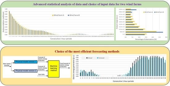
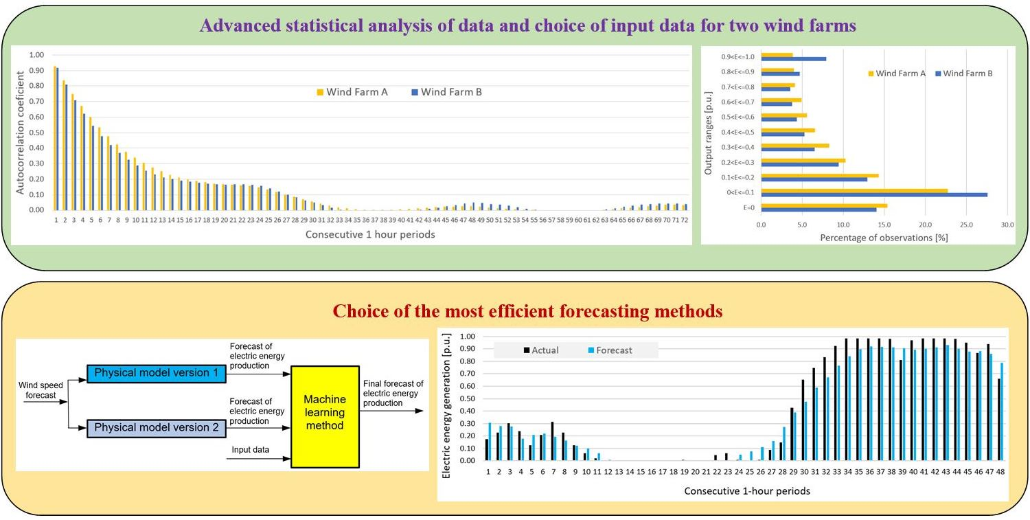
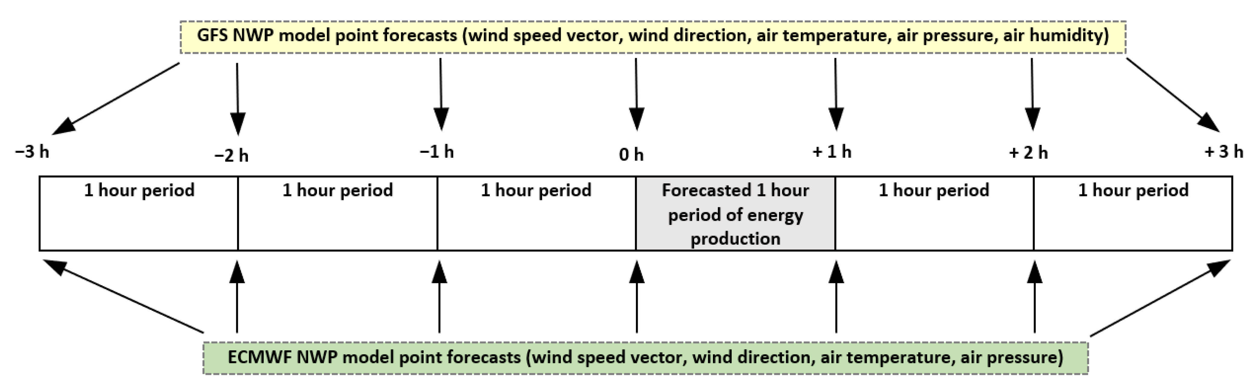
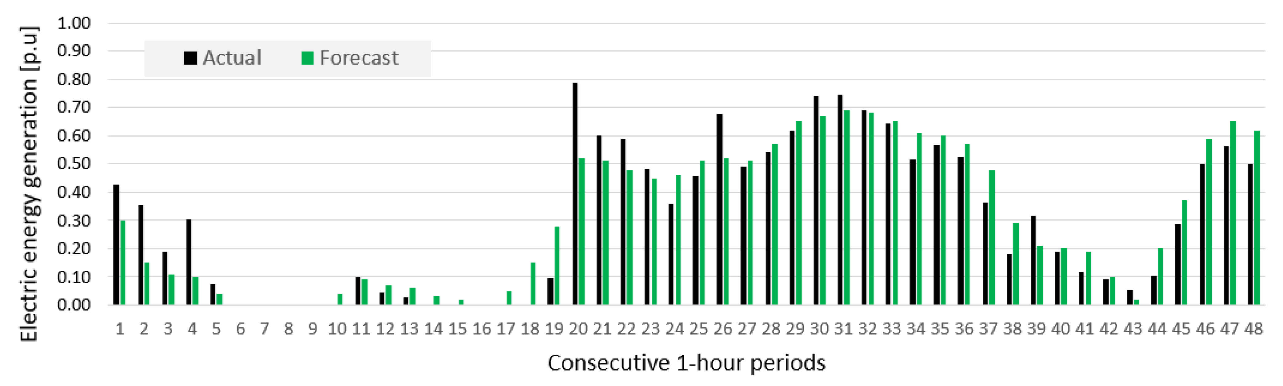
The remainder of this paper is organized as follows: Section 2.1 presents statistical analysis of times series and NWP data for two wind farms. The importance of the available basic input data and additional input data is discussed in Section 2.2 and Section 2.3. Section 3 describes prediction methods employed and Section 4 gives evaluation criteria for assessment of forecasting quality. Extensive analysis of the results and their discussion is in Section 5. Section 6 summarizes the whole research providing the main conclusions. References are listed at the end of this paper.

2. Data

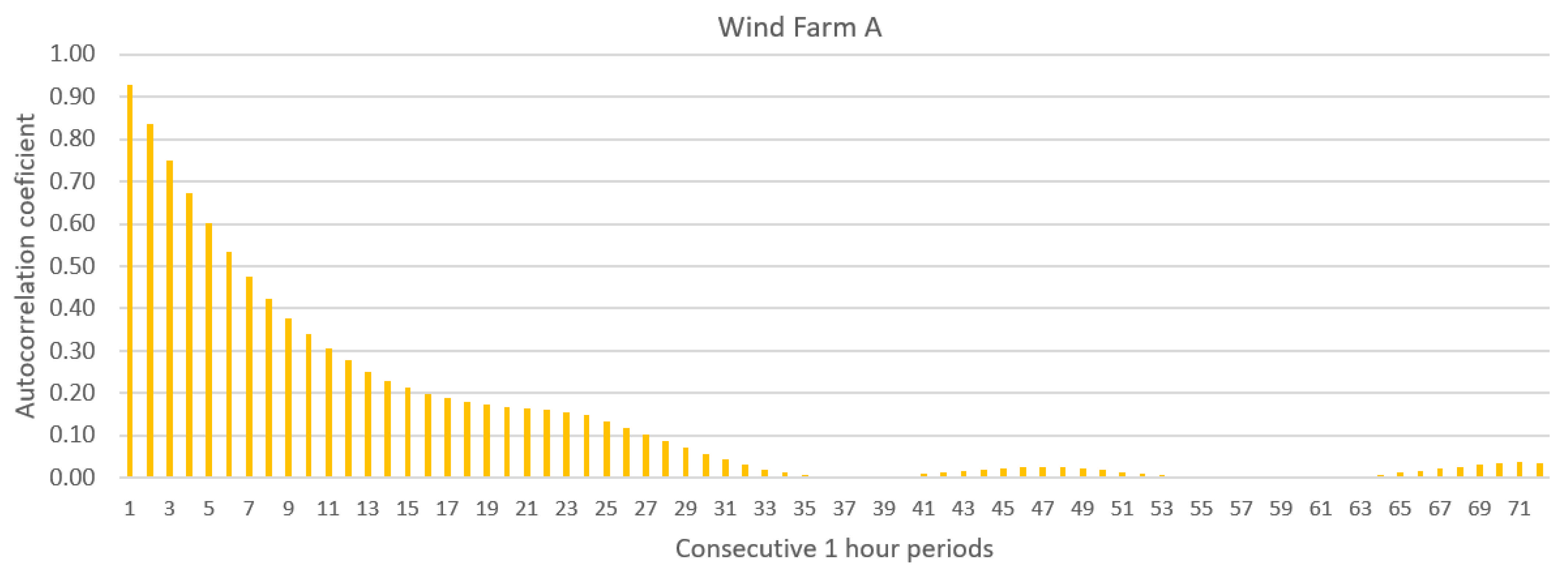
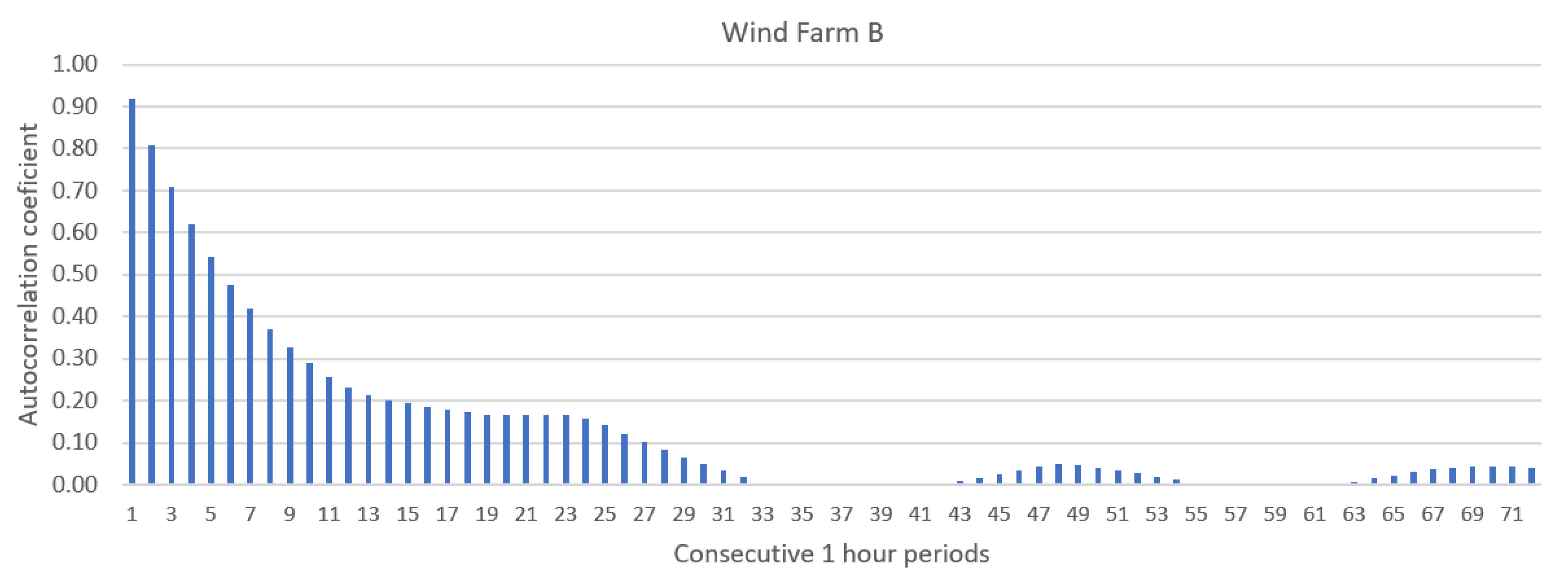
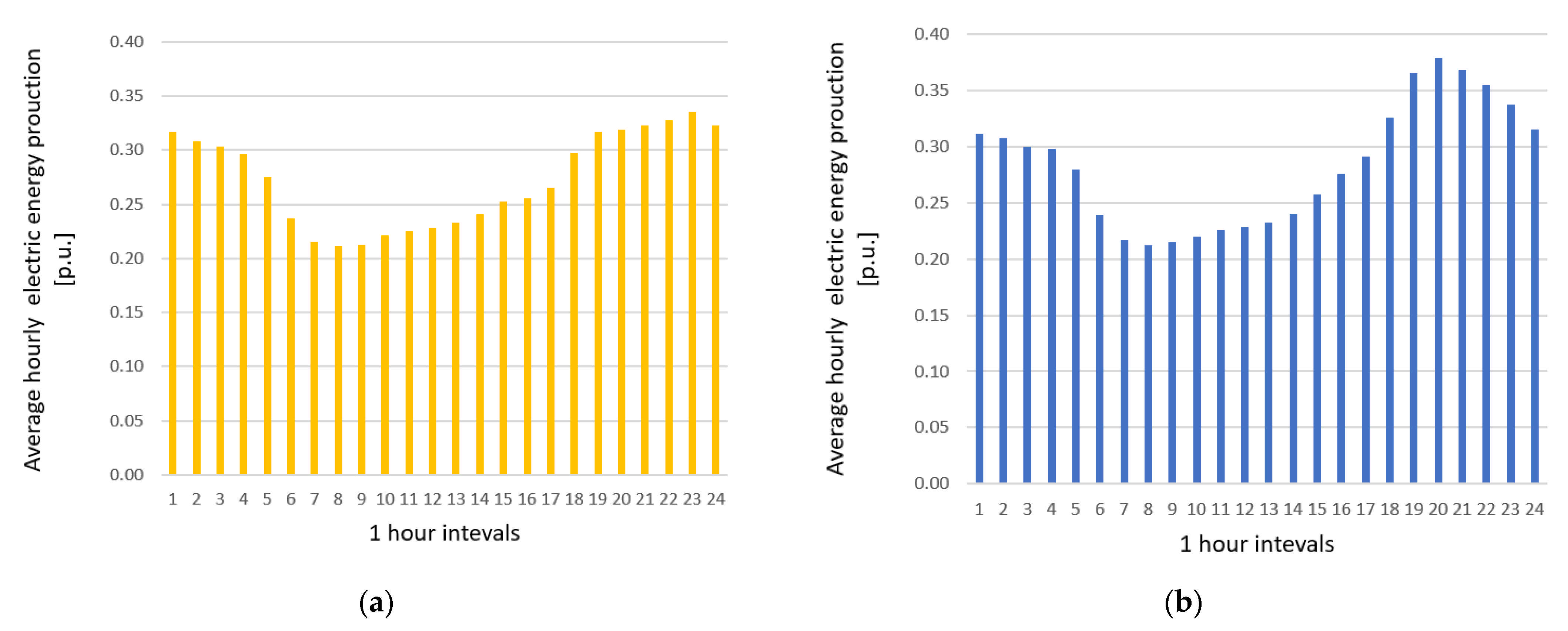
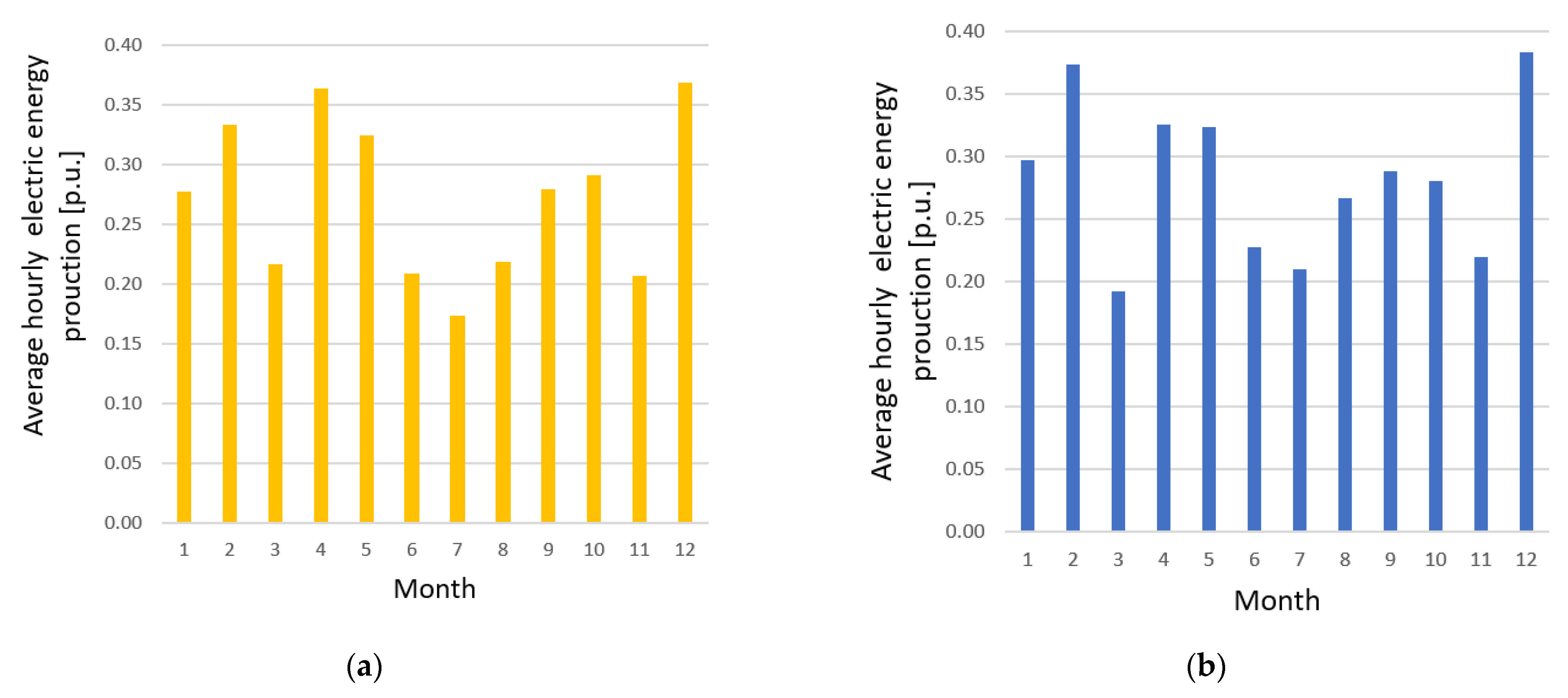
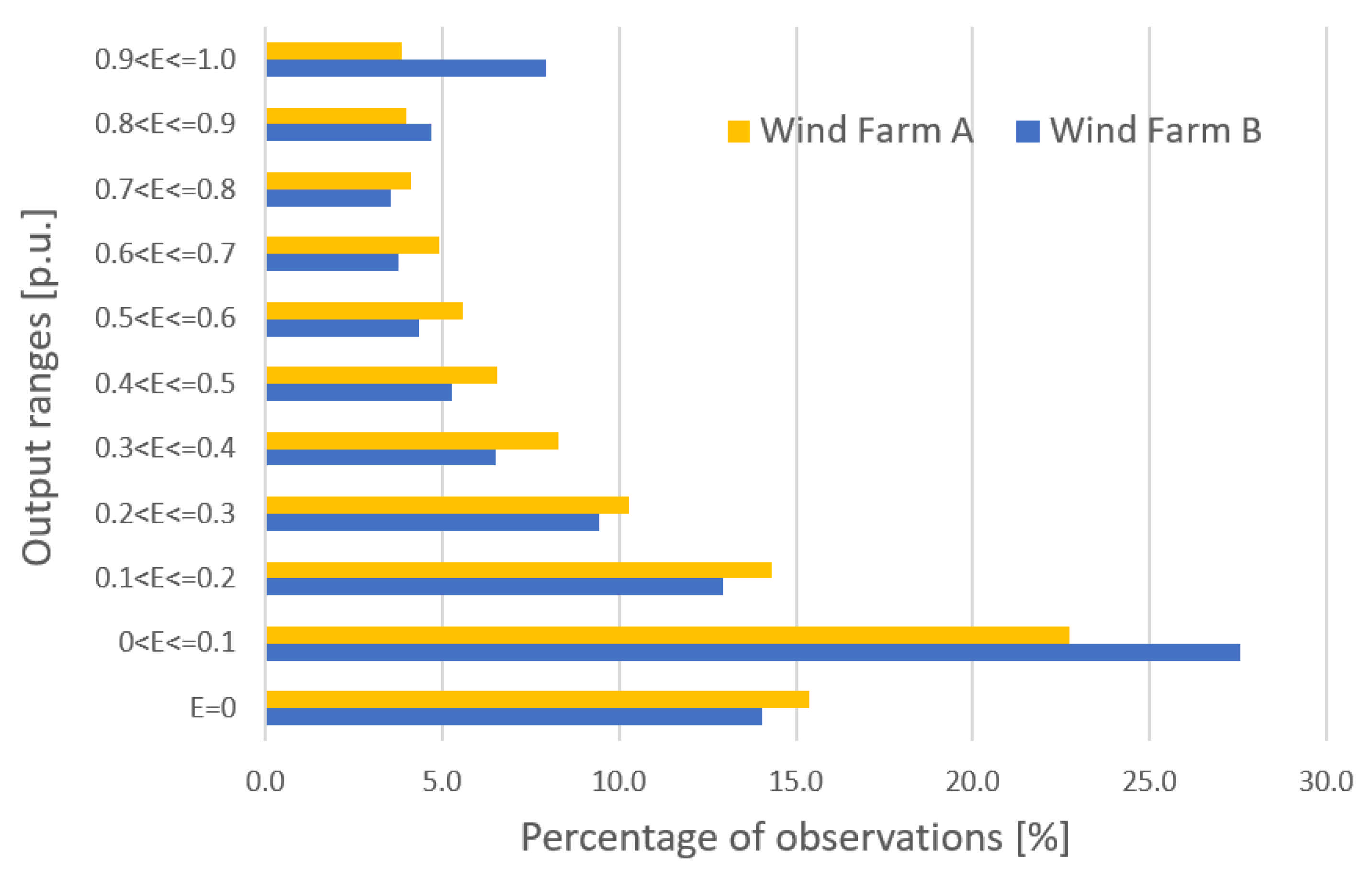
2.1. Statistical Analysis

For statistical analyses, data acquired for two medium-sized European wind farms (A and B) were used. The range of the acquired data was identical for both farms and spanned from 4 April 2017 to 10 October 2019, with about 29 months in total. Rated powers for Farms A and B were 50 MW and 48.3 MW, respectively.
The following data were available for analysis:
  • Wind farm generation time series (forecasted variable);
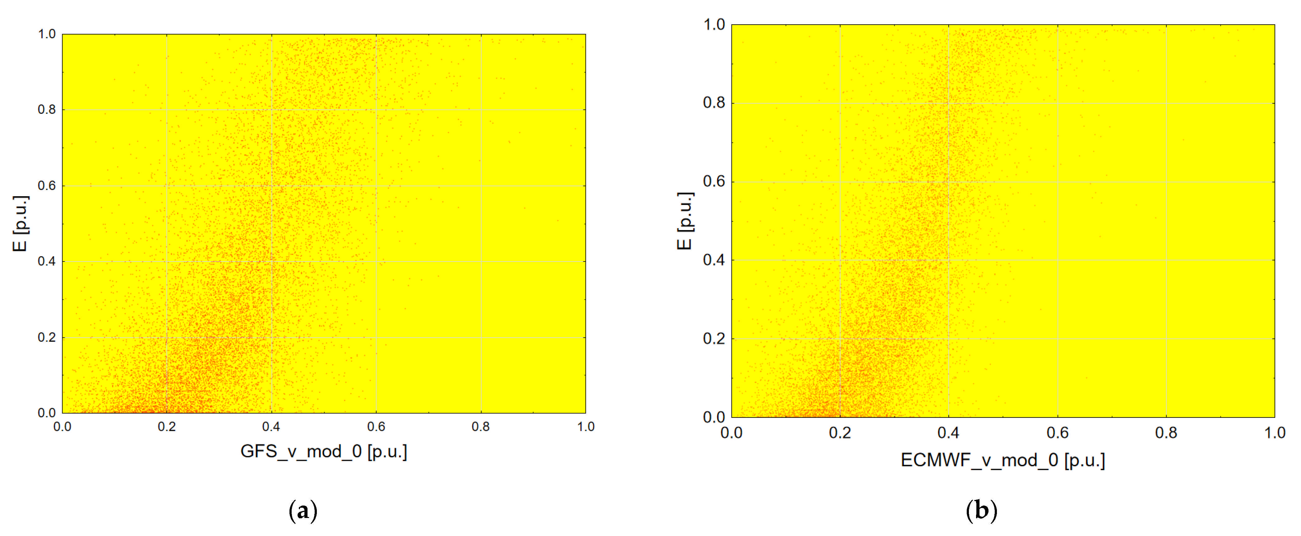
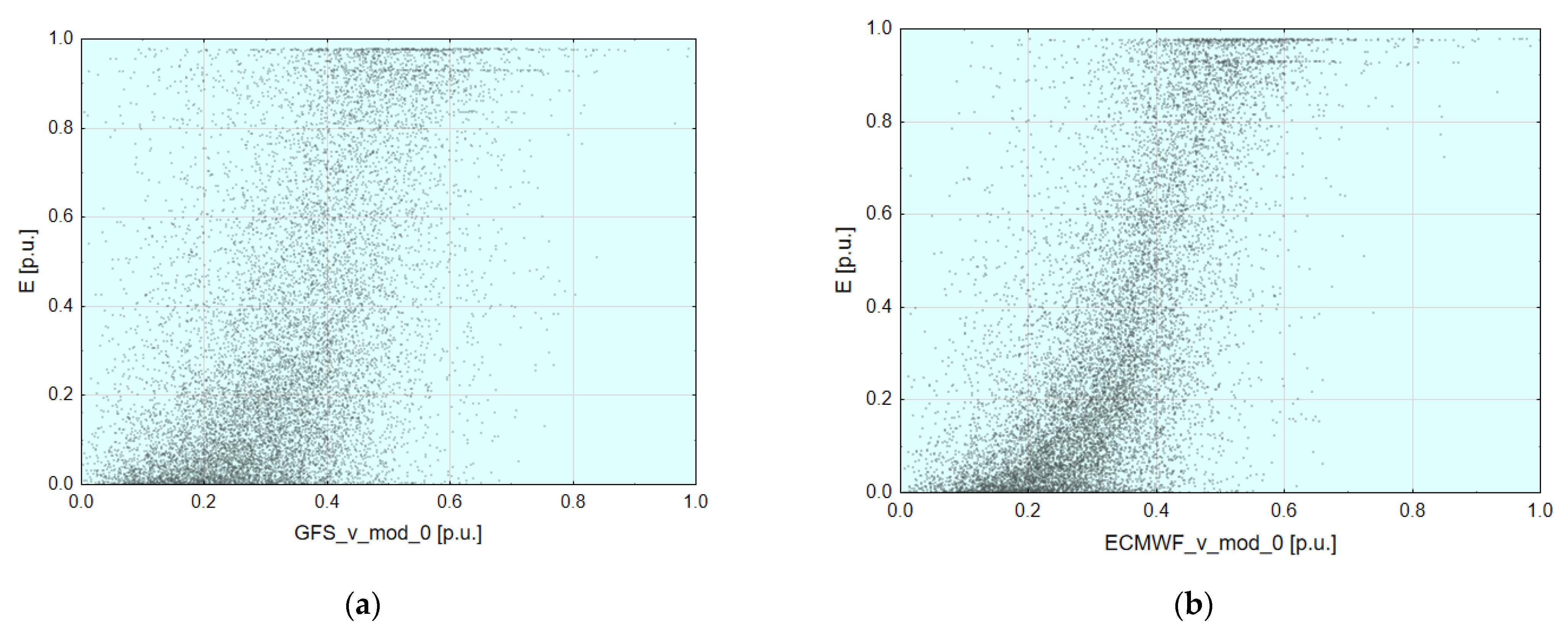
  • Weather forecasts for wind farms location.
Records of actual meteorological parameters were not available; hence, GFS and ECMWF NWP models were used for our research instead. For ECMWF, the archived high-resolution atmospheric model was chosen (HRES) [34]. The GFS model was supplied by the Interdisciplinary Modelling Center, Warsaw University (ICM UW) [35,36]. Both models make it possible to use 4 forecast runs per day (at 0/6/12/18 UTC) with 1 h resolution and maximal horizon of 240 h. Time resolution of HRES changes, however, to a 3 h interval after 90 h horizon and to 6 h after 144 h horizon. For GFS, only the first interval change appears after reaching the 120 h horizon. For each wind farm, only weather forecasts corresponding to the respective spatial point were used. Weather source points for the ECMWF model were chosen as the points nearest to the ones appearing in a dense 1/8 × 1/8-degree grid. The same method was applied to GFS with its native spatial resolution of 0.25 × 0.25 degrees.
Data from both time series of electric energy production (Farm A and Farm B) were normalized separately for anonymization to relative units (1 relative unit is equal to the rated power of the wind farm). However, each time series of NWP forecasts data was normalized using min–max scaling.
Table 1 shows descriptive statistics for time series of hourly electric energy generated by the Wind Farm A and Wind Farm B considered here. Percentage distribution of electric energy generation for both wind farms is shown in Figure 1. The analysis of electric energy generation percentiles shows that values very close to 0 made up more than 25% of both time series samples. Usually, energy generation was within the range of (0–0.1) [p.u.] for both time series samples.
Calculated autocorrelation coefficient (ACF) of hourly generation in both time series shows a little daily periodicity. Autocorrelation coefficients quickly decrease for the following hours of the first day. For both time series, all autocorrelation coefficients are statistically significant (5% significance level) up to 3 days back (72 prior observations). Autocorrelation function (ACF) of the Wind Farm A energy generation time series is presented in Figure 2. However, autocorrelation function (ACF) of the Wind Farm B energy generation time series is presented in Figure 3.
Figure 4 shows daily variability of hourly energy production [p.u.] of Wind Farms A and B. Arithmetic means of hourly energy generations for each hour of the day were calculated based on data span from 4 April 2017 to 28 September 2018 (18 months in total), with omitting test period datetimes—1 October 2018 to 1 October 2019. For the same periods, mean arithmetic hourly generations were calculated for each month, with the averaging of values for the months occurring two times. Pearson linear correlation coefficient between the data is equal to 0.950. Daily variability of electric energy generation of both wind farms is similar.
Figure 5 shows seasonal variability of electrical energy generation of Wind Farms A and B. Pearson linear correlation coefficient between the data is equal to 0.922. Seasonal variability of electric energy generation of both wind farms is similar.
Figure 6 presents dispersion diagrams—relationships between wind speed forecasts [p.u.] for the beginning of a 1 h period of energy generation and actual production of electrical energy [p.u.] from Wind Farm A for 2 different NWP models (GFS and ECMWF). Figure 7 contains similar diagrams for Wind Farm B. For both figures, points are slightly more concentrated for the ECMWF model (cases b). All dispersion diagrams indicate a non-linear relationship between wind speed and the yield of electricity. The exact shape corresponding approximately to the shape of the wind turbine power curve typical for a single turbine cannot be well seen on the diagram due to low concentration of data points. Both of the observed disadvantageous phenomena result probably from the following reasons:
  • Data include wind speed forecasts instead of actual, recorded values;
  • Wind speed forecasts are momentary values for a given hour and actual wind speed usually changes during a 1 h period;
  • Data come from very large wind farms with turbines scattered across vast territory with varying orography. For single wind turbines, data would probably be much more concentrated.
For both wind farms, extreme outliers were treated as unreliable samples, and further removed from data. This can be due to incorrect readings, missing data or scheduled/unscheduled shutdowns of at least a part of the wind farm. Only extreme, rarely occurring outliers were removed from the data, since big errors of wind speed prediction certainly must occur in a 24 h forecast horizon. A scenario with null wind speed forecast and non-zero electricity generation could be given as an example of NWP inaccuracy.

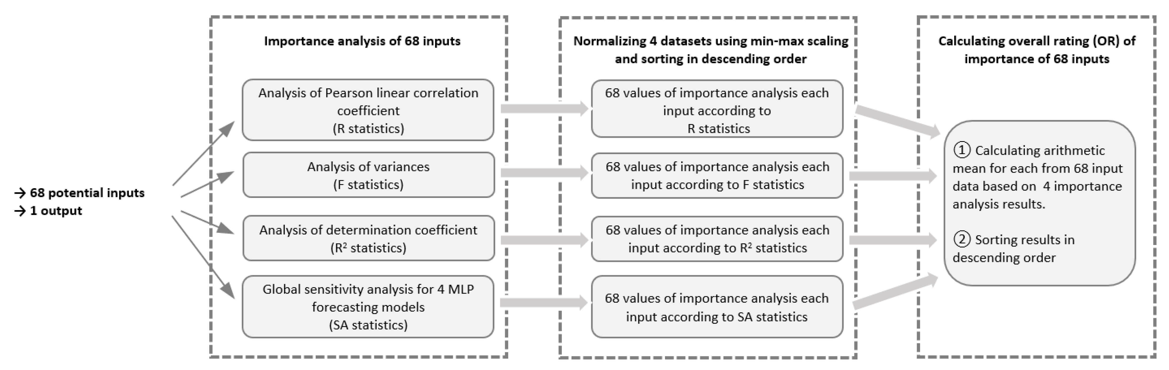
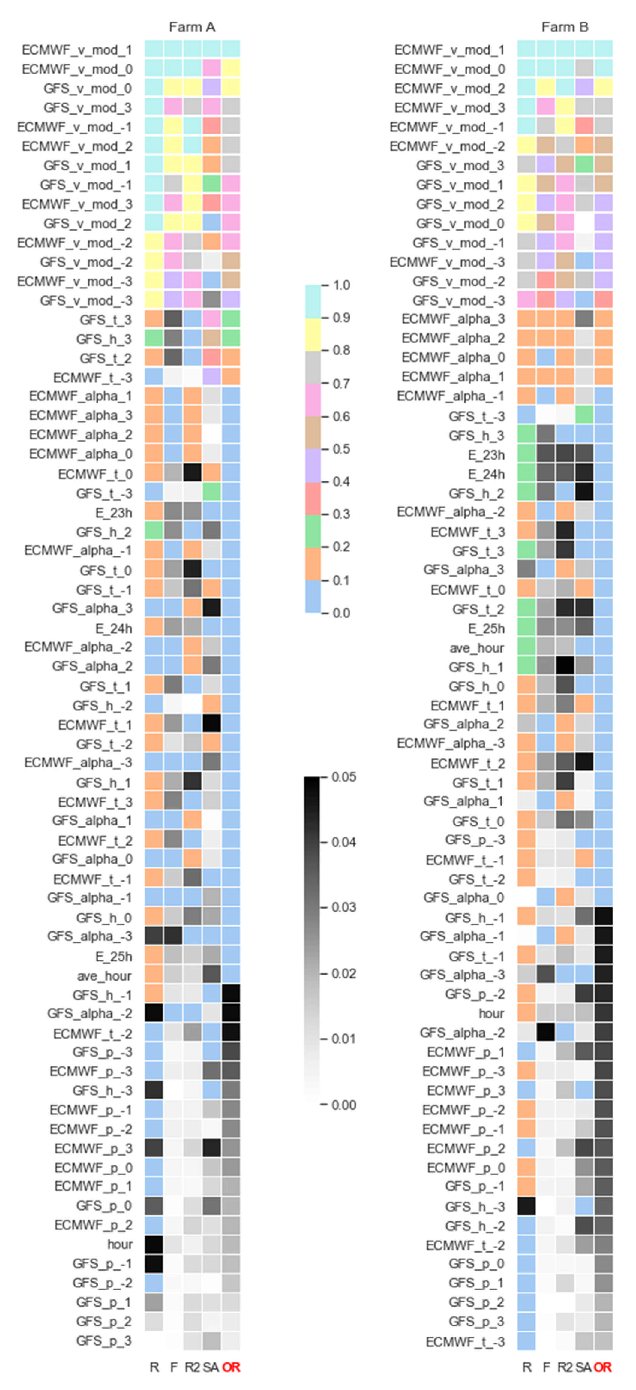
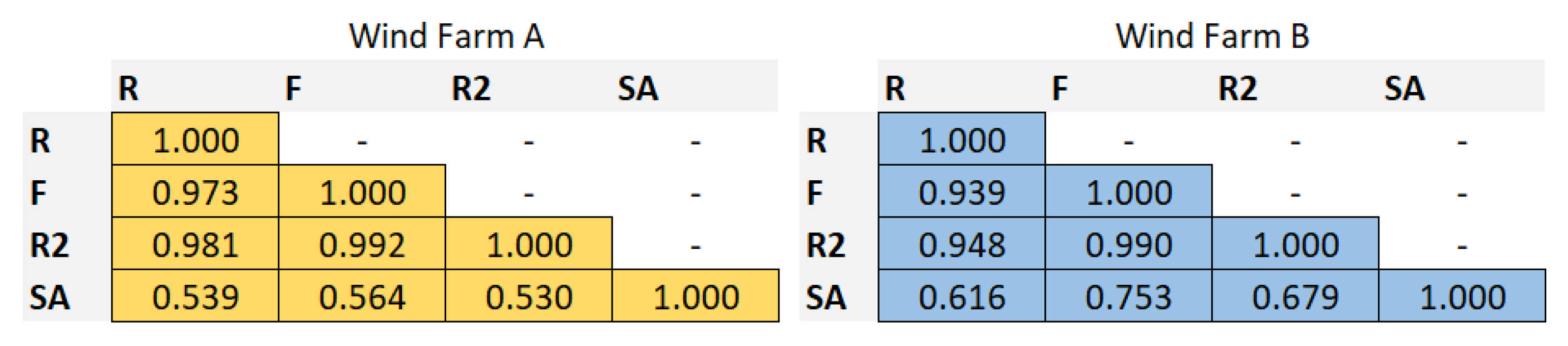
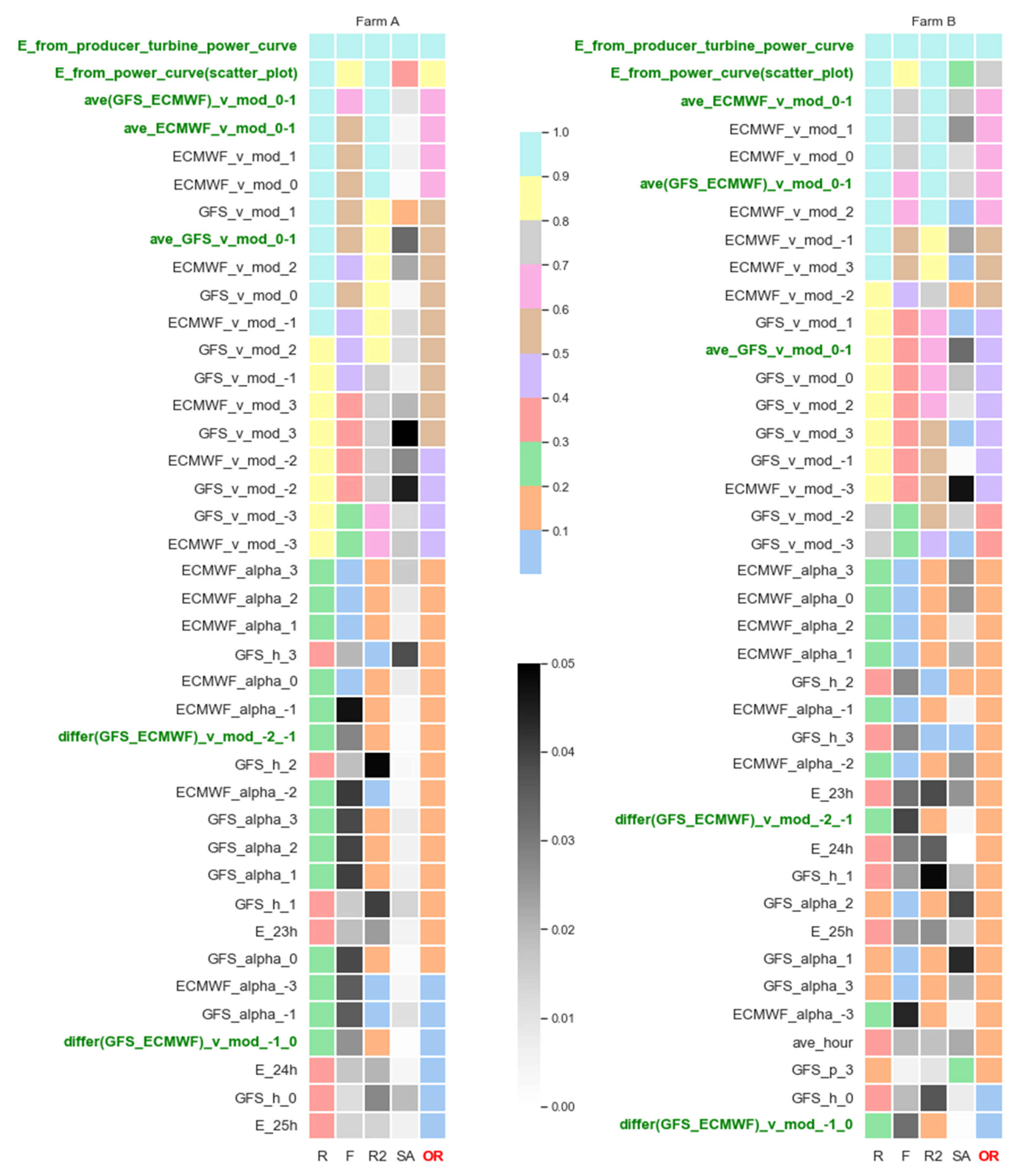
2.2. Analysis of Importance of Available Basic Input Data for Forecasting Methods

A detailed description of the available basic set of potential input variables for forecasting models is presented in Table 2. Figure 8 presents time points (momentary values time lags) of point weather forecasts from GFS and ECMWF models (input data) in relation to periods of electricity generation.
To identify the most important inputs for prediction models, extensive sensitivity analysis was performed for both wind farms. All of the 68 potential input variables that had been acquired were included. Comparison of the importance of input variables for both farms made it possible to draw general conclusions about the validity of use of given variables in predictions of electricity generation from large wind farms. Figure 9 presents consecutive steps of this analysis. Global Sensitivity Analysis (SA statistics) in the MLP network was performed for 4 models. Each trained model had 68 input variables and 1 output variable (electricity generation), 40, 50, 60, 70, and 80 (5 models) hidden neurons, used the BFGS learning algorithm, hyperbolic tangent hidden layer activation function, and linear output layer activation function. After training each MLP model, GSA was performed and the importance of each input variable was computed. Next, for each input, the overall rating was calculated as the arithmetic mean of 4 results of global sensitivity analysis obtained from each MLP model.
Results of sensitivity analysis for potential input variables of prediction models are shown in Figure 10. The most important input variables are definitely wind speed forecasts, notably, the ones closest to the 1 h energy generation period. ECMWF NWP forecasts turned out higher in ranking than GFS forecasts, while the least important input variables were predictions of atmospheric pressure.
The importance of INPUT variables varied between 4 analytic methods used here for both value of metrics and position in importance ranking. The most differing results came from the SA method due to the non-linear modelling (MLP network) used in that method. The remaining analytic methods used linear modelling; hence, their results were similar. Figure 11 contains the interrelationship matrix (Pearson linear correlation coefficients) between 4 analytic methods used to determine the importance of input variables.

2.3. Analysis of Importance of Additional Input Data Created

A detailed description of an additional set of potential input variables for forecasting models, derived from mathematical transformation of basic data, is presented in Table 3. Additional input data are created to verify their potential usefulness and importance in the forecasting process. Wind speed forecasts using either one or both NWP models are averaged to reduce the random component. Percentage differences between averaged wind speed/atmospheric pressure point forecasts for respective pairs of hourly lags are computed to include additional information about the dynamics for wind speed/atmospheric pressure in the model. Physical model (turbine power curve) prognosis is another additional information. A third-order polynomial is used to approximate the power curve, while averaged wind speeds with lag 0 and 1 from time bounds of the predicted periods are inputs to this model.
Figure 12 shows the results of importance analysis of the additional input data created. The analysis was performed according to steps in Figure 3, the same as for the basic input data case, and used 68 basic input variables (described in Table 2) and 13 additional inputs (described in Table 3). Figure 12 presents partial results-40 best input variables out of the total of 81. Studies have shown that additional input data, in particular forecasts from physical models and average values of predictions, are highly valuable as prediction model explanatory data, as additional input data usually rank high in terms of importance (OR metrics). Moreover, similar results for both wind farms show the universality of our procedure of the construction of additional input data. As the next step, it was verified whether additional data can be advantageous for different methods of electricity generation forecasting.

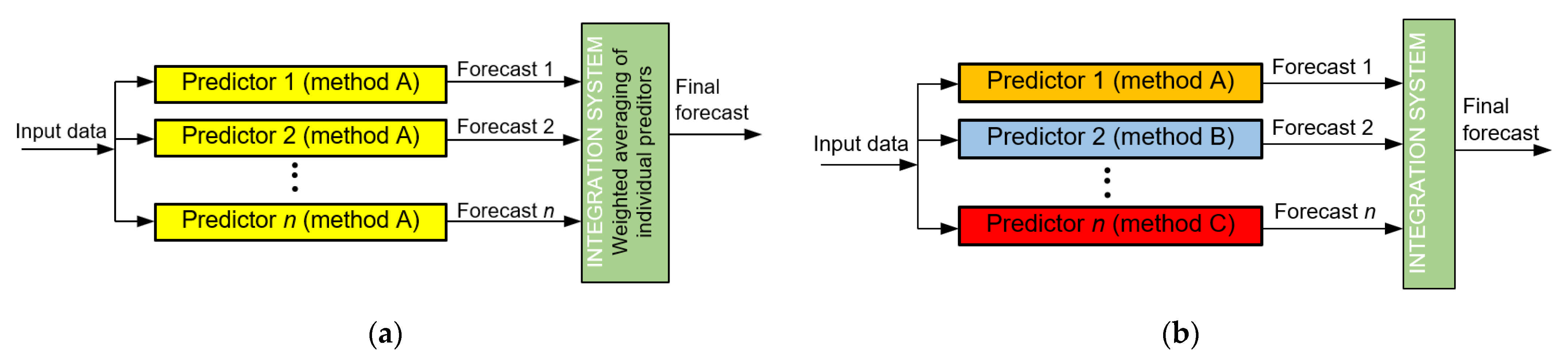
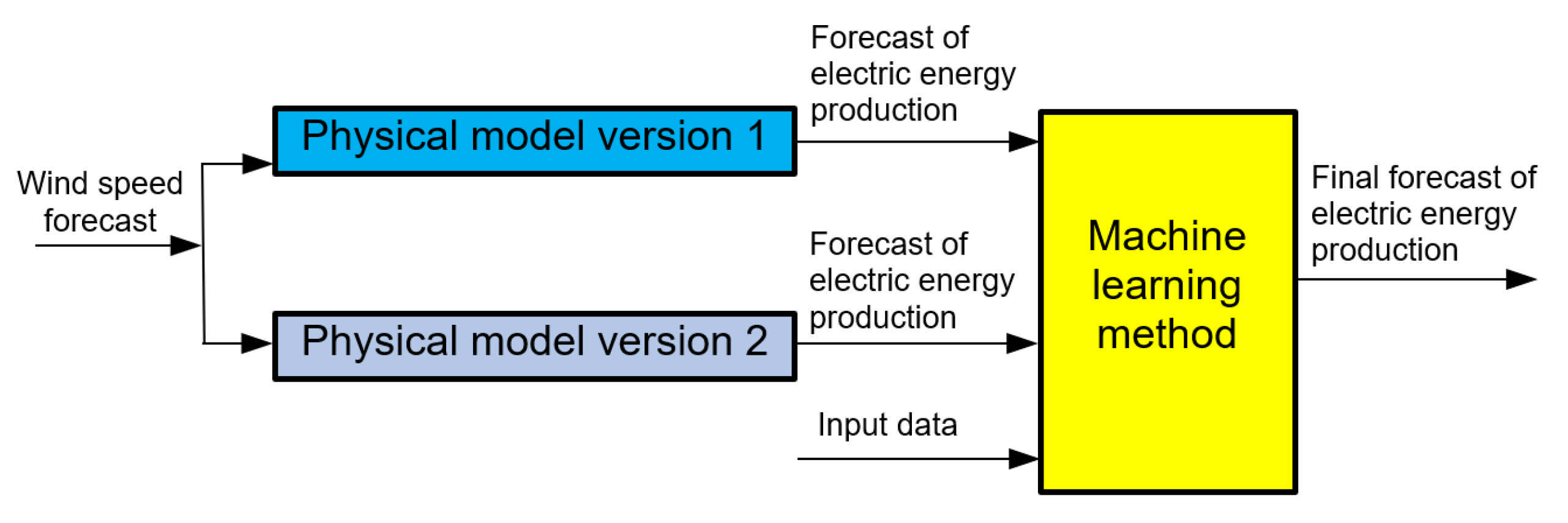
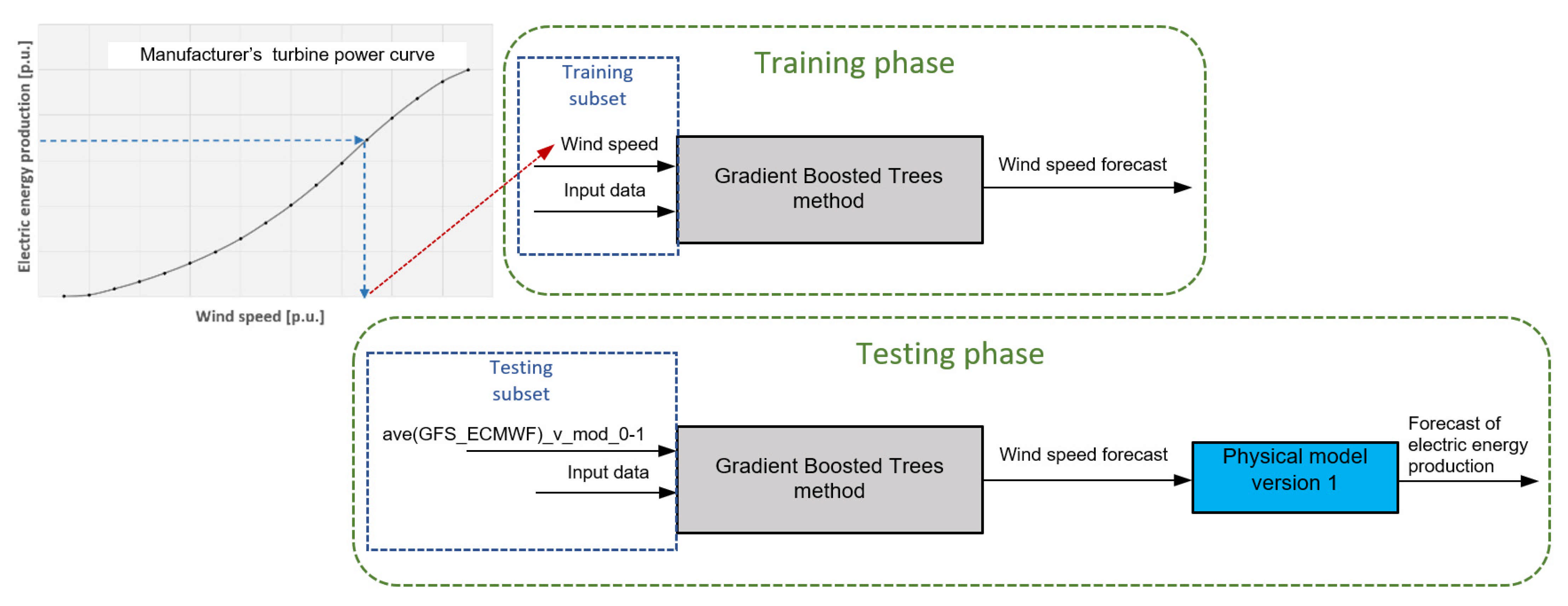
3. Forecasting Methods

This section includes the description of proposed forecasting methods. The research used both single methods as well as advanced ensemble and hybrid methods. Described the Persistence Model is a benchmark for the quality of other, more advanced forecasting methods.
Single methods, using only one individual predictor, are addressed next. The general scheme is presented in Figure 13.
Persistence model. The naïve model is the simplest model in forecasting. In the Persistence Model, the forecast generation value is the same as the actual energy generation value from the same hour the day before. Forecasts are calculated by Formula (1):
y ^ t = y t 24
where y ^ t —forecast electric energy generated by wind farm for hour t and y t 24 n —energy generation for period lagged by t – 24 from forecast period t.
Physical Model. This forecasting model of generated hourly power is a function of wind speed. The function is in the form of the 3rd-order polynomial. Two different methods were utilized to form 3rd-degree polynomial separately for Wind Farm A and Wind Farm B.
  • Physical model version 1. The polynomial of degree 3 is estimated based on turbine power curve data from the manufacturer’s catalogue (turbine power for wind speeds with 1 m/s steps). For input data below and above cut-in for each turbine, the forecast is equal to zero. The input data depend on variant (ave(GFS_ECMWF)_v_mod_0-1, ave_ECMWF_v_mod_0-1 or ave_GFS_v_mod_0-1).
  • Physical model version 2. The polynomial of degree 3 is estimated based on the scatter plot between electric energy production and wind speed forecasts (ave(GFS_ECMWF)_v_mod_0-1). For input data below and above cut-in for each turbine, the forecast value is equal to zero. The input data are ave(GFS_ECMWF)_v_mod_0-1.
K-Nearest Neighbours Regression. KNNR is a non-parametric method used for regression problems [37]. The input of the model contains the k-closest training examples in the feature space. The output of KNNR model is the property value for the object. Property value is the average of the values of k-nearest neighbours. Hyperparameter—the value of k (the number of nearest neighbours) needs searching for the appropriate value. The other hyperparameter for tuning is the choice of the distance metric.
Neural Network, Type MLP—Multi-layer Perceptron is a classical type of ANN. Widely used over decades, it proved its applicability as an effective non-linear or linear global approximator [13,38]. It is a feedforward ANN usually with an input layer, one or two hidden layers, and an output layer. Originally, it used the backpropagation algorithm for supervised learning. During years of development, other optimisation algorithms were applied for MLP learning, among them, the BFGS method that was chosen as the learning algorithm in our research. The number of neurons in hidden layer(s) was decided to be the main hyperparameter for tuning.
Support Vector Regression. Support Vector Machine for regression (SVR) transforms the classification task into regression by defining hyperparameter width ε tolerance region around the destination [39]. Hyperparameters of SVR for tuning are the following: regularization constant C, tolerance ε, and parameter s of the Gaussian kernel.
Deep Neural Network Type LSTM. The main difference between LSTM and traditional RNNs is LSTM’s internal built format. Its hidden layers contain 3 gates, namely, input, forget, and output gate. This solution allows to control the flow of information and allows to deal with problems such as gradient explosion and vanishing, and taking long-term dependencies into account [10]. A typical LSTM network contains an input layer followed by up to two hidden layers finished by an output layer with dropout layers possible between layers. The dropout mechanism’s goal is to prevent overfitting by keeping node in network with Bernoulli distribution probability [40]. The LSTM model contains (among others) the following hyperparameters: the number of hidden layers and neurons in them, activation function in each layer, number of training epochs, batch size, dropout degree, type of model optimizer, and learning rate.
Ensemble methods, using more than one individual predictor and supported by a simple or more complex integration system of individual forecasts, are addressed next. The simplest integration system is weighted averaging of individual predictors. The general scheme of establishing an ensemble of predictors is presented in Figure 14. The ensemble method can use the same type of methods as predictors (e.g., Random Forest, Gradient-Boosted Trees) or different types of predictors (e.g., single Machine Learning methods as predictors.
Random Forest Regression. RF is an ensemble method based on many single decision trees (the same type of models). In the regression task, the prediction in a single decision tree is the average target value of all instances associated with the single leaf node [41]. The final prediction is the average value of all n single decision trees. The regularization hyperparameters depend on the algorithm used, but generally restricted are among others: the maximum depth of a single decision tree, maximum number of levels in each decision tree, minimum number of data points placed in a node before the node is split, minimum number of data points allowed in a leaf node and maximum number of nodes. The number of predictors for each of the n single decision trees is made by the random choice of k predictors from all available n predictors [41,42].
Gradient-Boosted Trees for Regression. Gradient boosting refers to an ensemble method that can combine several weak learners into a strong learner [41]. GBT works by sequentially adding predictors (the same type of models) to the ensemble, each one correcting its predecessor. The method tries to fit the new predictor into the residual errors made by the previous predictor. The final prediction is the average value from all n single decision trees. In comparison with random forest, this method has one additional hyperparameter—learning rate, which scales the contribution of each tree [42,43].
Ensemble Averaging Without Extremes. The method developed by the authors of this study involves the deletion of the minimum and maximum forecast from the set of n single predictors (different types of methods) before each calculation of single final forecasts, being an average of forecasts from n-2 single predictors. The deletion is executed 24 times for each forecast separately. The choice predictors in the ensemble is based on the similar levels of forecasting error and mutually independent operation [9]. The final forecast result is calculated by Formula (2).
y ^ i = 1 n 2 ( k = 1 s y ^ i k min { y ^ i k } max { y ^ i k } )
where i is the forecast point, y ^ i is the final forecast value, y ^ i k is the forecasted value by predictor number k, and n is the number of predictors in the original ensemble before the removal of the outputs of predictors yielding extreme forecasts from the set of results.
Weighted Averaging as an Integrator of Ensemble based on nMAE and R. It integrates the results of selected predictors (different types of methods) into the final verdict of the ensemble. The final forecast is defined as the average of the results generated by all n predictors in the ensemble and is calculated by Formula (3) [9,39]. This method reduces the variance of forecast errors. Predictors are included in the ensemble based on two important elements:
  • time series of the residues from forecasts should be most distant from each other (small R values);
  • the smallest nMAE errors on the validation subset.
y ^ i = 1 n j = 1 n y ^ i j
where i is the prediction point, y ^ i is the final predicted value, y ^ i j is the predicted value by predictor number j, and n is the number of hybrid predictors in the ensemble.
Hybrid methods, using two or more different methods connected in series, are addressed next.
Machine learning method with additional input data from two Physical models. This hybrid method is a cascade of two different Physical models (version 1 and version 2) with one of the five ML methods (GBT, SVR, KNNR, MLP, or LSTM). ML component uses both forecasts of electric energy production as an additional input. The general scheme of this hybrid method is presented in Figure 15.
Physical model version 1 with input data as wind speed forecast from Gradient-Boosted Trees method. This hybrid method consists of the Gradient-Boosted Trees method connected in series with Physical Model Version 1. The GBT method predicts wind speed, while Physical Model Version 1 forecasts electric energy production. Physical Model Version 1 yielded smaller errors than the MLP and GBT methods considered here. The training and testing subsets differ from each other. The training subset uses wind speed based on the manufacturer’s reversed turbine power curve (third-order polynomial) as additional input. This allows the method to learn effective wind speed corresponding to actual values of electric energy production. In turn, the testing subset uses ave(GFS_ECMWF)_v_mod_0-1 as its additional input, since electric energy production, and thus effective wind speed, would be unobtainable during the operational work of the models. The concept of this hybrid methods is based on the assumption that GBT will learn better on a training subset containing a precise estimate of wind speed than on one containing wind speed forecasts with a large random component. The general scheme of this hybrid method is presented in Figure 16.
A summary description of thirteen tested forecasting methods is shown in Table 4. The listed methods include four types of ensemble methods, two types of hybrid ones, and seven single methods. Six methods (single/ensemble) are machine learning (ML) methods, including one deep learning method.
Additional expert correction of forecasts. Since wind turbines produce no power below the lower and above the upper limits of wind speed, a unique expert correction method is proposed. Obviously, without verification, the use of the correction would be unjustified, as it applies to wind speed forecasts with a large random component instead of real-world wind speeds. Due to that, its effectiveness and validity are verified for the selected group of methods providing best forecasts. A robust wind estimator ave(GFS_ECMWF)_v_mod_0-1 is used as a conditional variable for the method to adjust for bias of singular NWP models. For wind speed forecasts—ave(GFS_ECMWF)_v_mod_0-1 below cut-in and above cut-out wind speeds for wind turbine, forecast electric energy production is corrected to zero. The final prediction with expert correction is calculated by Formula (4).
E ^ i = { E ^ i   f o r   v m i n v ^ i v m a x 0   f o r   v ^ i v m i n 0   f o r   v ^ i v m a x
where E ^ i is the predicted value (electric energy production), v ^ i is the predicted wind speed (ave(GFS_ECMWF)_v_mod_0-1) and v m i n and v m a x are cut-in and cut-out wind speeds of turbine.

4. Evaluation Criteria

Three evaluation criteria are used to test the performance of the methods, including normalized Root Mean Square Error (nRMSE), normalized Mean Absolute Error (nMAE) and normalized Mean Bias Error (nMBE).
Normalized Root Mean Square Error which is sensitive to large error values is calculated by Formula (5):
n R M S E = 1 c n o r m 1 n i = 1 n ( y ^ i y i ) 2
where y ^ i is the predicted value (electric energy production), y i is the actual value, c n o r m is the normalizing factor (rated power of wind farm), and n is the number of prediction points.
Normalized Mean Absolute Error is calculated by Formula (6). nMAE is a risk metric according to the expected value of the absolute error.
n M A E = 1 n i = 1 n 1 c n o r m | y ^ i y i | 100 %
Normalized Mean Bias Error (nMBE) captures average bias in prediction and is calculated by Formula (7). The forecasting method overestimates if nMBE > 0 or underestimates if nMBE < 0.
n M B E = 1 n i = 1 n 1 c n o r m ( y ^ i y i )
Errors nRMSE and nMAE are basic measures to evaluate the accuracy of proposed models, while nMBE is only auxiliary. In the process of forecasting electric energy production in a wind farm, the changes of nRMSE and nMAE have the same trend, and the smaller the two error values, the more accurate the prediction results. Both show random and systematic errors. A large gap between nMAE and nRMSE for the results of a method indicates that predicted values are extremely distant from the measured data [44,45].
The effectiveness of the forecasting approaches is found by considering the uncertainty and variability of forecasts [46]. For a comparative assessment of the performance test of the analysed methods, the Skill Score (SS) metric was used. The proposed Skill Score metric uses two error metrics—nRMSE and nMAE—and is calculated by Formula (8). Higher SS values are an indication of superior prediction quality.
S S = 1 2 [ ( 1 n M A E f o r e c a s t n M A E r e f e r e n c e ) + ( 1 n R M S E f o r e c a s t n R M S E r e f e r e n c e ) ]
where n M A E f o r e c a s t and n R M S E f o r e c a s t are errors of the analysed method, n M A E r e f e r e n c e and n R M S E r e f e r e n c e are errors of reference method (persistence method—naive model).

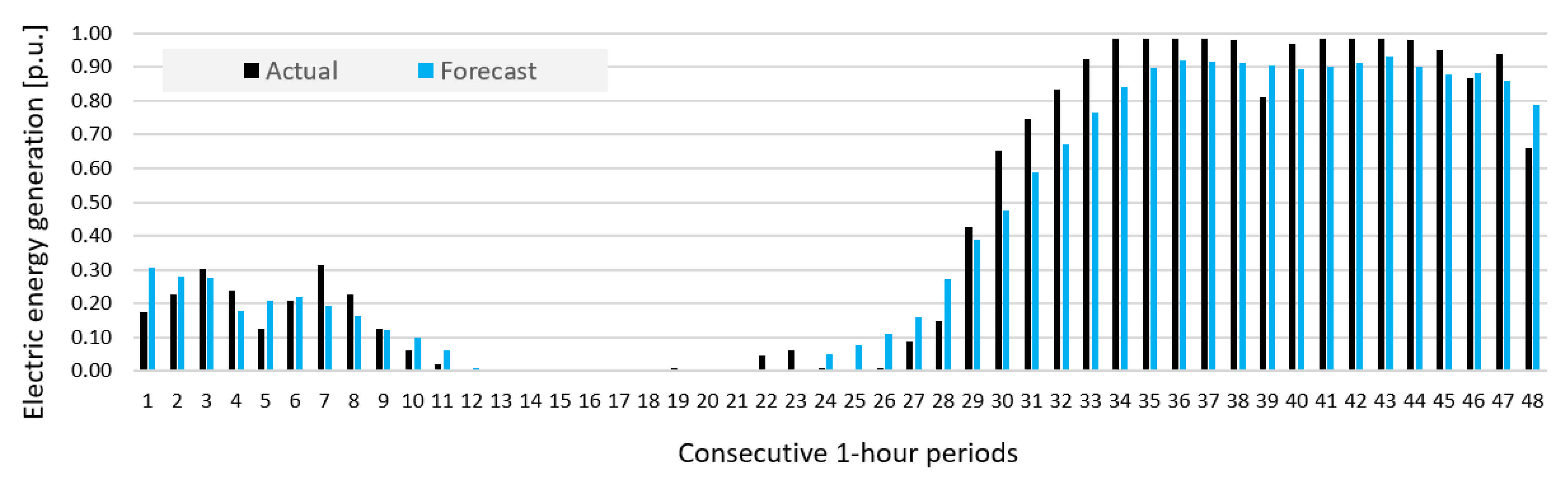
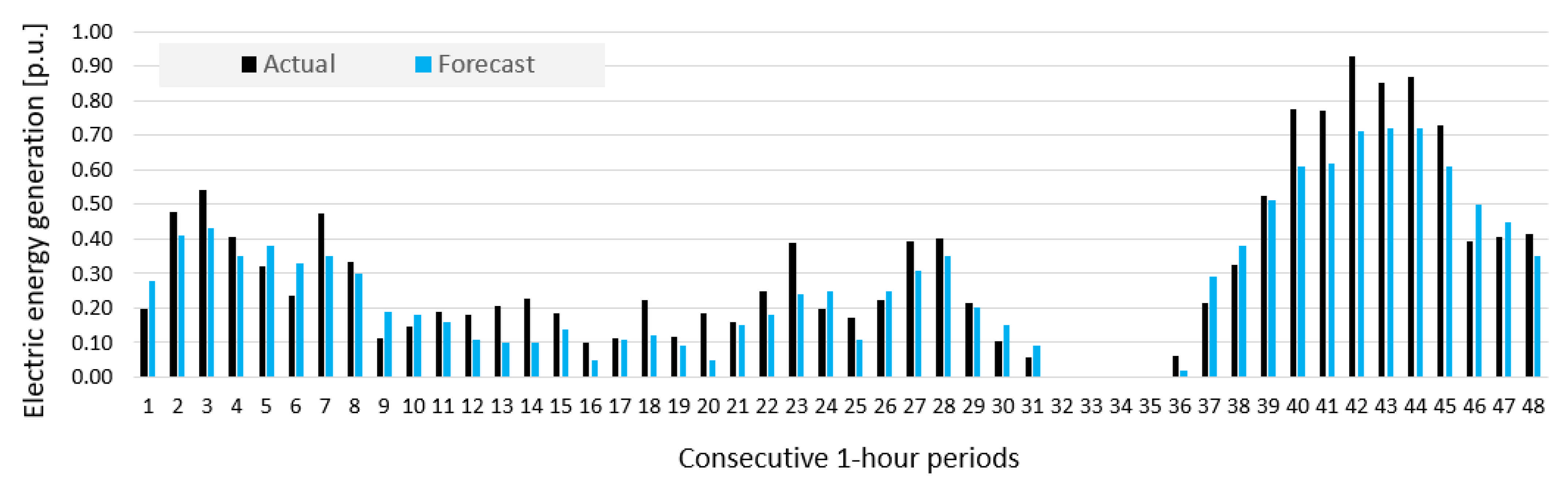
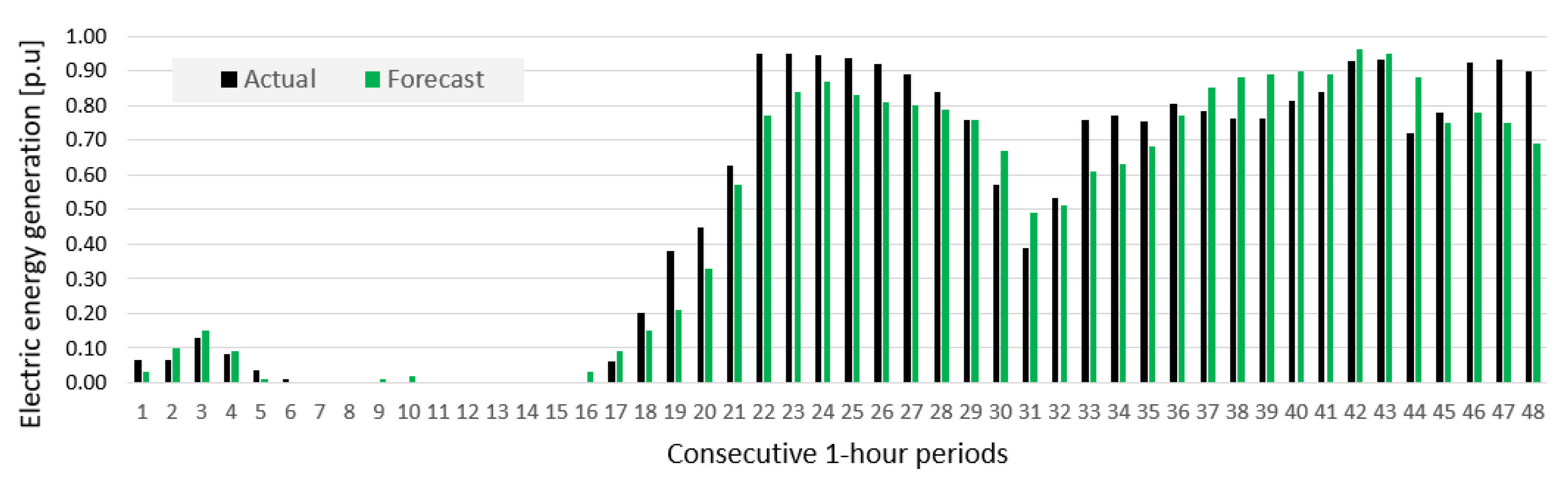
5. Results and Discussion

The range of the acquired data was identical for both wind farms and spanned from 4 April 2017 to 10 October 2019, with about 29 months in total. Data were divided into three subsets—training subset, validation subset, and test subset. The training and validation subsets for the period from 4 April 2017 to 30 September 2018 (17 months) were chosen at random (85% and 15%, respectively). The training subset is used for the estimation of model parameters. The validation subset is used for tuning hyperparameters of parts of methods. The last part of the data (from 1 October 2018 to 1 October 2019—12 months) constituted the test subset used for one-time final evaluation of the quality of specific prediction methods on data for all seasons.
Predictions were conducted sequentially, from single methods with a limited number of input variables to hybrid methods, to ensemble methods. Such procedure allows us to observe differences in the quality of results depending on the complexity of particular methods and the range of input variables used. Research was done in steps in order to verify different hypotheses, and find an optimal input dataset and the best group of prediction methods.
Step 1. Hypotheses verification:
  • Are the accuracies of two designed physical models different from each other?
  • Is it better to use one or two NWP models with wind speed forecasts for physical models?
Table 5 and Table 6 contains results of forecasts for A and B wind farms, respectively. Physical and Persistence (reference) Models were used for predictions.
Results of the two Physical Models indicate that PHYS_v1 was better fitted for both wind farms, while results for the NWP models were ambiguous. Although using only the GFS model was clearly the least favourable option, for Wind Farm A it was better to use both NWP models, while for Wind Farm B it was better to use the ECMWF model only. In comparison, the nMAE Persistence Model was twice as good as both Physical Models.
Step 2. Hypotheses verification:
  • Is it better to use NWP point forecasts for hourly lags: −3, 2, −1, 0, 1, 2, 3 (original contribution) as input data instead of the typically used lags 0, 1?
  • Is it better to use one or two NWP models as input data source?
To verify the above, a strong GBT method was used, recommended by multiple papers. Table 7 and Table 8 present the resulting forecasts for Wind Farms A and B using the proposed GBT method with different versions of NWP input data.
Research in step 2 demonstrated that the order of the results obtained with the same combination of input data was the same for both wind farms. Best accuracies were achieved by using both NWP models. The application of the novel and original idea of using point forecasts for hourly lags: −3, 2, −1, 0, 1, 2, 3 yields clearly better results than using typical 0, 1 lags. Like in Physical Models, in this case, forecasts for Wind Farm B were less accurate than for Wind Farm A. Preliminary studies analysing the importance of input data also indicated slightly lesser correlation between NWP forecasts for Wind Farm B than for Wind Farm A. The above findings were used in further research steps; hence, the subsequent versions of forecasts use both NWP models predictions and point forecasts for hourly lags: −3, 2, −1, 0, 1, 2, 3.
Step 3. This step is the main, most extensive and labour intensive part of research. Forecasts of energy production were obtained from different single, hybrid and ensemble models, including by original methods. To find proper hyperparameters for them, more than 300 hyperparameter combinations were tested using the Grid Search method. The lowest nMAE score on the validation range was used as the parameter selection criterion. Hyperparameter search ranges and their determined values for chosen methods are summarized in Table A1 in Appendix A. The described determinations were carried out to verify the following:
  • Which method group yields the lowest prediction errors (recommended methods) and does the Ensemble Averaging Without Extremes original method developed by us belong to the recommended methods?
  • Does the original proposition developed by us—additional input variables (see Table 3)—reduce the prediction error?
  • Does the original proposition developed by us—additional expert correction—reduce the prediction error?
Table 9 and Table 10 present forecasts for Wind Farms A and B resulting from the proposed single, ensemble and hybrid methods with different sets of input data. For the two best methods, results are shown with and without additional expert correction (see Formula (4)).
Tabular results were ordered by descending SS metric, which was taken as the main determinant of prediction quality, as it takes into account both nMAE and nRMSE errors.
Based on the results from Table 9 and Table 10, the following conclusions can be drawn regarding the proposed single, hybrid, and ensemble methods with different sets of input data:
  • Original method called “Ensemble Averaging Without Extremes” is the best for both wind farms (SS metric and nMAE error);
  • For “Ensemble Averaging Without Extremes”, the best fitted solution was to use an ensemble of 5 methods, while a 3-method ensemble was the best for “Weighted Averaging As an Integrator of Ensemble”;
  • Our original method “Additional Expert Correction” resulted in lower nMAE than for predictions without correction. For “Ensemble Averaging Without Extremes”, nMAE decreased by 0.42% for Wind Farm A and 0.92% for Wind Farm B;
  • Hybrid methods have worse accuracy measures of nMAE and nRMSE than ensemble methods for both wind farms;
  • Deep neural network LSTM is the best single method, MLP is the second best;
  • Original hybrid “Physical Model Version 1 With Input Data As Wind Speed Forecast from Gradient-Boosted Trees Method” turned out to be of less advantage than ensemble methods;
  • For most methods, using additional input data (numbers: 1A, 2A, 3A) reduced nMAE in comparison with using basic input data only (numbers: 1–68). KNNR was an exception as it yielded the lowest nMAE with a highly reduced number of input data variables;
  • Values of nMBE were very low for the analysed methods, which means there was no systematic error in predictions. The lowest nMBE for both wind farms was achieved with the RF Method;
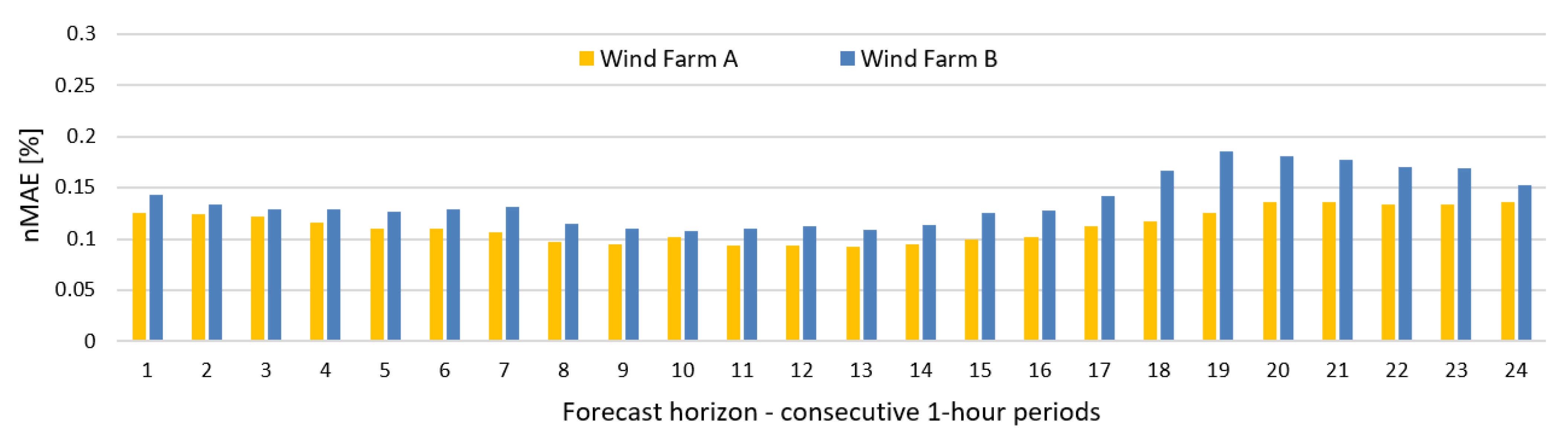
  • Prediction errors for Wind Farm B were bigger than for Wind Farm A, which was indicated by results of sensitivity analysis of potential input variables (see Figure 10).
Figure 17, Figure 18, Figure 19 and Figure 20 provides two forecasts of electric energy generation for Wind Farm A made by the best method with additional expert correction for the two following days of each season (from autumn to summer).
Figure 21, Figure 22, Figure 23 and Figure 24 provides two forecasts of electric energy generation for Wind Farm B made by the best method with additional expert correction for two following days of each season (from autumn to summer).
Figure 17, Figure 18, Figure 19, Figure 20, Figure 21, Figure 22, Figure 23 and Figure 24 show that energy generation of both wind farms in presented days (16 in total) is highly random. For some hours of certain days, generation is periodically close to its rated value, but for other hours generation is very low. There are also few hour periods of null generation. The lowest generations and predictions among the presented 16 days occurred for 4 days of summer months (Figure 20 and Figure 24). It should be noted that generation predictions have periods of both over- and under-forecasting. Most commonly, it can be observed on a few consequent samples of time series. Moreover, time series of generation predictions have slightly smoothened course due to using the ensemble method, as ensemble methods reduce the variance of forecasts. For “Ensemble Averaging Without Extremes”, additional removal of extreme forecasts occurs before average forecast calculation, which, in turn, further enhances the smoothening effect for generation prediction time series.
For both wind farms, additional analysis of nMAE error distribution was made. It concerned hourly periods of prediction using the best forecasting method of “Ensemble Averaging Without Extremes”. The goal of analysis was to determine whether error magnitude depends on forecast horizon (from 1 to 24 h) and time of the day. Figure 25 shows the graph of the forecast error (nMAE) depending on the forecast horizon for the test subset for Wind Farm A and Wind Farm B.
nMAE values presented in Figure 25 are visibly greater for Wind Farm B, which complies with the results from Table 9 and Table 10. nMAE error equals 11.3055% and 13.7552% for Wind Farm A and B, respectively. The distribution of error values shown in Figure 25 and the distribution of average production of energy in individual hours values shown in Figure 4a,b are very similar for both wind farms. For Wind Farm A, the correlation coefficient is equal to 0.9331, and for Wind Farm B, the correlation coefficient is equal 0.9291. Both autocorrelation coefficients are statistically significant (5% significance level). This phenomenon is related to a strong non-linear relationship between the energy forecast error and the wind speed forecast error. The aforementioned non-linear relationship results from the fact that the generation of energy in the wind source is a third-degree polynomial of the wind speed.

6. Conclusions

Using two wind farms for statistical analyses and forecasting considerably improves credibility of newly created effective prediction methods and conclusions. The results of the study are summarized below.
Original ensemble methods, developed for researching specific implementations, reduced errors of energy generation forecasts for both wind farms as compared to single methods. The best integration system for ensemble methods for accuracy measure nMAE is a new, original integrator developed for predictions, called “Ensemble Averaging Without Extremes” (method code INT_OUT_EXT), with five methods in the ensemble. The best integration system for ensemble methods for accuracy measure nRMSE is an original integrator developed for predictions called “Weighted Averaging As an Integrator of Ensemble” (method code INT_AVE) with three methods in the ensemble.
A new, original “Additional Expert Correction” reduced errors of energy generation forecasts for both wind farms. Deep neural network LSTM is the best single method, MLP is the second best, while using SVR, KNNR, and Physical model is less favourable for both wind farms. Hybrid methods have worse accuracy measures using nMAE and nRMSE than ensemble methods for both wind farms.
Using meteo forecasts from two NWP models (ECMWF and GFS) as input data yield better results than using a single NWP model. Using NWP point forecasts for hourly lags: −3, −2, −1, 0, 1, 2, 3 (original contribution) as input data is better than using typical lags 0, 1. Using additional input data created, especially input data numbers: 1A, 2A, 3A, reduces prediction errors of most methods in comparison with base input variables (input data numbers: 1–68).
For both wind farms, strong positive correlation was determined between distribution of energy production averages, in particular, hourly periods and distribution of prediction errors (nMAE). Identifying this relationship is valuable, practical information concerning the expected value of prediction error depending on the time of the day. The greater the average generation for a given hour, the greater the prediction error (nMAE) expected. For both analyzed wind farms, the greatest prediction errors are expected during evening hours, while the lowest errors are expected between 08:00 a.m. and 2:00 p.m.
Using original SS metric to compare prediction accuracy is useful, as it allows to incorporate both nMAE and nRMSE into final quality assessment. Both measures are important for the end user of the prediction, as the former is sensitive to reducing the average error, while the latter is sensitive to overforecasting and underforecasting.
More research is needed to verify, among other things, the following:
  • Does prediction accuracy depend on using forecasts from more than one spot of a medium-sized wind farm and how the accuracy of forecasts will be affected by other factors, i.e., data with higher time resolution, e.g., 15 min, using real measurements of weather as input data?
  • Can measurements and weather predictions be used to create a weather-error sensitive switching regime for models of ensembles?
  • Is it possible to reduce the level of high random component in predictions?
  • Will the proposed, original method of “Ensemble Averaging Without Extremes” be equally good for different types of RES predictions (e.g., photovoltaic systems and hydropower system)?

Author Contributions

Conceptualization, P.P., D.B.; methodology, P.P., D.B.; investigation, P.P., D.B. and M.K.; supervision, P.P.; validation, M.K., T.G.; writing, P.P., D.B., M.K. and T.G.; visualization M.K., P.P.; project administration, P.P. All authors have read and agreed to the published version of the manuscript.

Funding

This research was funded by The National Centre for Research and Development (Poland), Grant No. ID POIR.01.01.01-00-130/16 (to P.P., D.B., M.K.).

Institutional Review Board Statement

Not applicable.

Informed Consent Statement

Not applicable.

Data Availability Statement

Not applicable.

Conflicts of Interest

The authors declare no conflict of interest.

Abbreviations

The following abbreviations are used in this manuscript:
ACFAutocorrelation function
ANNArtificial Neural Network
BFGSBroyden–Fletcher–Goldfarb–Shanno algorithm
BPNNBack Propagation Neural Network
CNNConvolutional Neural Network
DNNDeep Neural Network
ECMWFEuropean Center for the Medium-Range Weather Forecast
ELMExtreme Learning Machine
ENNElman Neural Network
ESNEcho State Network
FFisher test
GBTGradient-Boosted Trees
GFSGlobal Forest System
GRUGated Recurrent Unit
HRESHigh-resolution atmospheric model
IECInternational Electrotechnical Commission
KNNRK-Nearest Neighbours Regression
LSTMLong short-term memory
MLMachine Learning
MLPMulti-Layer Perceptron
NARXNonlinear Autoregressive Exogenous Model
nMAEnormalized Mean Absolute Error
nMBEnormalized Mean Bias Error
NWPNumerical Weather Prediction
PSOParticle Swarm Optimization
p.u. Per unit
RPearson linear correlation coefficient
R2Determination coefficient
RESRenewable Energy Sources
RFRandom Forest
RNNRecurrent Neural Network
nRMSEnormalized Root Mean Square Error
SASensitivity analysis
SSSkill Score
SVRSupport Vector Regression
SVMSupport Vector Machine

Appendix A

Table A1. The results of hyperparameters tuning for chosen single, hybrid and ensemble methods for Wind Farm B.
Method CodeDescription of Method, the Name and the Range of Values of Hyperparameters Tuning and Selected Values
LSTM The number of hidden layers: 1–2, selected: 2, the number of neurons in hidden layer: 4–50, selected: 35–20,
the activation function in hidden layer: ReLU/sigmoid/tanh, selected hyperbolic tangent, the activation function in output layer: linear, learning algorithms ADAM, RMSprop, selected optimizer: ADAM, lr = 0.001, decay = 1 × 10⁻⁵, epochs: 1500, patience: 100, batch size: 128; shuffle: True. Dropout after each hidden layer: 0/0.2, selected dropout: 0.2
SVRRegression SVM: Type-1, Type 2, selected: Type-1, kernel type: Gaussian (RBF), the width parameter σ: 0.147, the regularization constant C, range: 1–20 (step 1), selected: 2, the tolerance ε, range: 0.01–1 (step 0.01), selected: 0.05.
PHYS(v1&v2)→KNNRDistance metrics: Euclidean, Manhattan, Minkowski, selected: Euclidean, the number of nearest neighbours k, range: 1–50, selected: 4.
MLPThe number of neurons in hidden layer: 10–80, selected 30, learning algorithm: BFGS, the activation function in hidden layer: linear, hyperbolic tangent, selected: hyperbolic tangent, the activation function in output layer: linear.
GBT Considered max depth: 2/4/6/10, selected depth: 6; trees number: 100/200/400, selected number: 100; learning rate: 0.1/0.01/0.001,
selected: 0.1
RFThe number of predictors chosen at random: 30, 35, 40, 45, 50, 55, 60, selected 35 number of decision trees: 1–500, selected: 385. Stop parameters: maximum number of levels in each decision tree: 5, 10, 20, selected 10, minimum number of data points placed in a node before the node is split: 100, 200, 300, selected 200, min number of data points allowed in a leaf node: 10, maximum number of nodes: 100.

References

  1. Liu, H.; Chen, C.; Lv, X.; Wu, X.; Liu, M. Deterministic wind energy forecasting: A review of intelligent predictors and auxiliary methods. Energy Convers. Manag. 2019, 195, 328–345. [Google Scholar] [CrossRef]
  2. Yildiz, C.; Acikgoz, H.; Korkmaz, D.; Budak, U. An improved residual-based convolutional neural network for very short-term wind power forecasting. Energy Convers. Manag. 2021, 228, 113731. [Google Scholar] [CrossRef]
  3. Duan, J.; Wang, P.; Ma, W.; Tian, X.; Fang, S.; Cheng, Y.; Chang, Y.; Liu, H. Short-term wind power forecasting using the hybrid model of improved variational mode decomposition and Correntropy Long Short-term memory neural network. Energy 2021, 214, 118980. [Google Scholar] [CrossRef]
  4. Abedinia, O.; Lotfi, M.; Bagheri, M.; Sobhani, B.; Shafiekhah, M.; Catalao, J.P.S. Improved EMD-Based Complex Prediction Model for Wind Power Forecasting. IEEE Trans. Sustain. Energy 2020, 11, 2790–2802. [Google Scholar] [CrossRef]
  5. Memarzadeh, G.; Keynia, F. A new short-term wind speed forecasting method based on fine-tuned LSTM neural network and optimal input sets. Energy Convers. Manag. 2020, 213, 112824. [Google Scholar] [CrossRef]
  6. Liu, B.; Zhao, S.; Yu, X.; Zhang, L.; Wang, Q. A Novel Deep Learning Approach for Wind Power Forecasting Based on WD-LSTM Model. Energies 2020, 13, 4964. [Google Scholar] [CrossRef]
  7. Wang, C.; Zhang, H.; Ma, P. Wind power forecasting based on singular spectrum analysis and a new hybrid Laguerre neural network. Appl. Energy 2020, 259, 114139. [Google Scholar] [CrossRef]
  8. Sun, Z.; Zhao, S.; Zhang, J. Short-Term Wind Power Forecasting on Multiple Scales Using VMD Decomposition, K-Means Clustering and LSTM Principal Computing. IEEE Access 2019, 7, 166917–166929. [Google Scholar] [CrossRef]
  9. Piotrowski, P.; Kopyt, M.; Baczyński, D.; Robak, S.; Gulczyński, T. Hybrid and Ensemble Methods of Two Days Ahead Forecasts of Electric Energy Production in a Small Wind Turbine. Energies 2021, 14, 1225. [Google Scholar] [CrossRef]
  10. Sun, M.; Feng, C.; Zhang, J. Multi-distribution ensemble probabilistic wind power forecasting. Renew. Energy 2020, 148, 135–149. [Google Scholar] [CrossRef]
  11. Chen, C.; Liu, H. Medium-term wind power forecasting based on multi-resolution multi-learner ensemble and adaptive model selection. Energy Convers. Manag. 2020, 206, 112492. [Google Scholar] [CrossRef]
  12. Du, P. Ensemble Machine Learning-Based Wind Forecasting to Combine NWP Output With Data From Weather Station. IEEE Sustain. Energy 2019, 10, 2133–2141. [Google Scholar] [CrossRef]
  13. Chen, J.; Zhu, Q.; Li, H.; Lin, Z.; Shi, D.; Li, Y.; Duan, X.; Liu, Y. Learning Heterogeneous Features Jointly: A Deep End-to-End Framework for Multi-Step Short-Term Wind Power Prediction. IEEE Trans. Sustain. Energy 2020, 11, 1761–1772. [Google Scholar] [CrossRef]
  14. Shahid, F.; Zameer, A.; Mehmood, A.; Raja, M.A.Z. A novel wavenets long short term memory paradigm for wind power prediction. Appl. Energy 2020, 269, 115098. [Google Scholar] [CrossRef]
  15. Su, H.-Y.; Huang, C.-R. Enhanced Wind Generation Forecast Using Robust Ensemble Learning. IEEE Trans. Smart Grid 12.1 2021, 2, 912–915. [Google Scholar] [CrossRef]
  16. Saini, V.K.; Kumar, R.; Mathur, A.; Saxena, A. Short term forecasting based on hourly wind speed data using deep learning algorithms. In Proceedings of the 2020 3rd International Conference on Emerging Technologies in Computer Engineering: Machine Learning and Internet of Things (ICETCE), Jaipur, India, 7–8 February 2020; pp. 1–6. [Google Scholar] [CrossRef]
  17. Ahmadi, A.; Nabipour, M.; Mohammadi-Ivatloo, B.; Amani, A.M.; Rho, S.; Piran, M.J. Long-Term Wind Power Forecasting Using Tree-Based Learning Algorithms. IEEE Access 2020, 8, 151511–151522. [Google Scholar] [CrossRef]
  18. Kisvari, A.; Lin, Z.; Liu, X. Wind power forecasting A data-driven method along with gated recurrent neural network. Renew. Energy 2021, 163, 1895–1909. [Google Scholar] [CrossRef]
  19. Ouyang, T.; Huang, H.; He, Y.; Tang, Z. Chaotic wind power time series prediction via switching data-driven modes. Renew. Energy 2020, 145, 270–281. [Google Scholar] [CrossRef]
  20. Li, L.L.; Zhao, X.; Tseng, M.L.; Tan, R.R. Short-term wind power forecasting based on support vector machine with improved dragonfly algorithm. J. Clean. Prod. 2020, 242, 118447. [Google Scholar] [CrossRef]
  21. Wang, X.; Li, P.; Yang, J. Short-term Wind Power Forecasting Based on Two-stage Attention Mechanism. IET Renew. Power Gener. 2019, 14, 297–304. [Google Scholar] [CrossRef]
  22. Yuan, X.; Chen, C.; Jiang, M.; Yuan, Y. Prediction interval of wind power using parameter optimized Beta distribution based LSTM model. Appl. Soft Comput. 2019, 82, 105550. [Google Scholar] [CrossRef]
  23. Niu, Z.; Yu, Z.; Tang, W.; Wu, Q.; Reformat, M. Wind power forecasting using attention-based gated recurrent unit network. Energy 2020, 196, 117081. [Google Scholar] [CrossRef]
  24. Hu, H.; Wang, L.; Lv, S.X. Forecasting energy consumption and wind power generation using deep echo state network. Renew. Energy 2020, 154, 598–613. [Google Scholar] [CrossRef]
  25. Yu, R.; Liu, Z.; Li, X.; Lu, W.; Ma, D.; Yu, M.; Wang, J.; Li, B. Scene learning: Deep convolutional networks for wind power prediction by embedding turbines into grid space. Appl. Energy 2019, 238, 249–257. [Google Scholar] [CrossRef] [Green Version]
  26. Hu, T.; Wu, W.; Guo, Q.; Sun, H.; Shi, L.; Shen, X. Very short-term spatial and temporal wind power forecasting A deep learning approach. CSEE J. Power Energy Syst. 2020, 6, 434–443. [Google Scholar] [CrossRef]
  27. Wang, Z.; Zhang, J.; Zhang, Y.; Huang, C.; Wang, L. Short-Term Wind Speed Forecasting Based on Information of Neighboring Wind Farms. IEEE Access 2020, 8, 16760–16770. [Google Scholar] [CrossRef]
  28. Yin, H.; Ou, Z.; Huang, S.; Meng, A. A cascaded deep learning wind power prediction approach based on a two-layer of mode decomposition. Energy 2019, 189, 116316. [Google Scholar] [CrossRef]
  29. Lin, Z.; Liu, X. Wind power forecasting of an offshore wind turbine based on high-frequency SCADA data and deep learning neural network. Energy 2020, 201, 117693. [Google Scholar] [CrossRef]
  30. Medina, S.V.; Ajenjo, U.P. Performance Improvement of Artificial Neural Network Model in Short-term Forecasting of Wind Farm Power Output. J. Mod. Power Syst. Clean Energy 2020, 8, 484–490. [Google Scholar] [CrossRef]
  31. Tang, B.; Chen, Y.; Chen, Q.; Su, M. Research on Short-Term Wind Power Forecasting by Data Mining on Historical Wind Resource. Appl. Sci. 2020, 10, 1295. [Google Scholar] [CrossRef] [Green Version]
  32. Piotrowski, P.; Baczyński, D.; Kopyt, M.; Szafranek, K.; Helt, P.; Gulczyński, T. Analysis of forecasted meteorological data (NWP) for efficient spatial forecasting of wind power generation. Electric Power Systems Research 2019, 175, 105891. [Google Scholar] [CrossRef]
  33. De Mattos Neto, P.S.G.; de Oliveira, J.F.L.; de O. Santos Júnior, D.S.; Siqueira, H.V.; Marinho, M.H.N.; Madeiro, F. An adaptive hybrid system using deep learning for wind speed forecasting. Inf. Sci. 2021, 581, 495–514. [Google Scholar] [CrossRef]
  34. Atmospheric Model high resolution 10-day forecast (Set I—HRES). Available online: https://www.ecmwf.int/en/forecasts/datasets/set-i (accessed on 15 January 2021).
  35. NCEP Products Inventory. Available online: https://www.nco.ncep.noaa.gov/pmb/products/gfs/ (accessed on 15 January 2021).
  36. Available online: https://mapy.meteo.pl (accessed on 15 January 2021).
  37. Dudek, G.; Pełka, P. Forecasting monthly electricity demand using k nearest neighbor method. Przegląd Elektrotechniczny 2017, 93, 62–65. [Google Scholar]
  38. Dudek, G. Multilayer Perceptron for Short-Term Load Forecasting: From Global to Local Approach. Neural Comput. App. 2019, 32, 3695–3707. [Google Scholar] [CrossRef] [Green Version]
  39. Osowski, S.; Siwek, K. Local dynamic integration of ensemble in prediction of time series. Bull. Pol. Ac. Tech. 2019, 67, 517–525. [Google Scholar]
  40. Piotrowski, A.P.; Napiorkowski, J.J.; Piotrowska, A.E. Impact of deep learning-based dropout on shallow neural networks applied to stream temperature modelling. Earth-Sci. Rev. 2020, 201, 103076. [Google Scholar] [CrossRef]
  41. Parol, M.; Piotrowski, P.; Kapler, M.; Piotrowski, M. Forecasting of 10-Second Power Demand of Highly Variable Loads for Microgrid Operation Control. Energies 2021, 14, 1290. [Google Scholar] [CrossRef]
  42. Géron, A. Hands-on Machine Learning with Scikit-Learn, Keras, and TensorFlow, 2nd ed.; O’Reilly Media, Inc.: Sevastopol, CA, USA, 2019. [Google Scholar]
  43. Hastie, T.; Tibshirani, R.; Friedman, J.H. The Elements of Statistical Learning. Data Mining, Inference, and Prediction, 2nd ed.; Springer: Berlin/Heidelberg, Germany, 2009. [Google Scholar]
  44. Zhao, Y.; Ye, L.; Li, Z.; Song, X.; Lang, Y.; Su, J. A novel bidirectional mechanism based on time series model for wind power forecasting. Appl. Energy 2016, 177, 793–803. [Google Scholar] [CrossRef]
  45. Shahram, H.; Xiaolei, L.; Zi, L.; Saeid, L. A Critical Review of Wind Power Forecasting Methods—Past, Present and Future. Energies 2020, 13, 3764. [Google Scholar] [CrossRef]
  46. Barcons, J.; Avila, M.; Folch, A. Diurnal cycle RANS simulations applied to wind resource assessment. Wind Energy 2019, 22, 269–282. [Google Scholar] [CrossRef] [Green Version]
Figure 1. Percentage of time-series observations in particular generation ranges.
Energies 15 01252 g001
Figure 2. Autocorrelation function (ACF) of the Wind Farm A energy generation time series.
Energies 15 01252 g002
Figure 3. Autocorrelation function (ACF) of the Wind Farm B energy generation time series.
Energies 15 01252 g003
Figure 4. (a) Daily variability of hourly energy production of Wind Farm A; (b) Daily variability of hourly energy production of Wind Farm B.
Energies 15 01252 g004
Figure 5. (a) Seasonal variability of electrical energy production of Wind Farm A; (b) Seasonal variability of electrical energy production of Wind Farm B.
Energies 15 01252 g005
Figure 6. (a) Relationship between wind speed forecast from GFS NWP model and electricity generation from Wind Farm A; (b) Relationship between wind speed forecast from ECMWF NWP model and electricity generation from Wind Farm A.
Energies 15 01252 g006
Figure 7. (a) Relationship between wind speed forecast from GFS NWP model and electricity generation from Wind Farm B; (b) Relationship between wind speed forecast from ECMWF NWP model and electricity generation from Wind Farm B.
Energies 15 01252 g007
Figure 8. Relationship between time lags of GFS and ECMWF forecasts and periods of electricity generation.
Energies 15 01252 g008
Figure 9. Consecutive steps of potential input data sensitivity analysis of made with 4 different methods and Overall Rating (OR).
Energies 15 01252 g009
Figure 10. Results of sensitivity analysis of potential input variables for prediction models for Wind Farm A and Wind Farm B: 4 analysis methods and final Overall Rating (OR).
Energies 15 01252 g010
Figure 11. Interrelationship matrix (Pearson linear correlation coefficients) between 4 methods used to determine the importance of input variables.
Energies 15 01252 g011
Figure 12. Results of sensitivity analysis of potential input variables including additional input data created for prediction models for Wind Farm A and Wind Farm B: 4 analysis methods and final Overall Rating (OR). Figure contains 40 best inputs out of 81. Names of additional inputs are marked green.
Energies 15 01252 g012
Figure 13. General structure of single method.
Energies 15 01252 g013
Figure 14. (a) General structure of ensemble method with the same type of methods as individual predictors; (b) General structure of ensemble method with different types of methods as individual predictors.
Energies 15 01252 g014
Figure 15. General structure of hybrid method—machine learning method with additional input data from two Physical models.
Energies 15 01252 g015
Figure 16. General structure of hybrid method—Physical model version 1 with input data as wind speed forecast from Gradient-Boosted Trees method.
Energies 15 01252 g016
Figure 17. Two forecasts of electric energy generation for Wind Farm A made by INT_OUT_EXT [GBT, RF, PHYS(v1&v2)→KNNR, MLP, LSTM] method with additional expert correction for two consecutive days of an autumn month (November).
Energies 15 01252 g017
Figure 18. Two forecasts of electric energy generation for Wind Farm A made by INT_OUT_EXT [GBT, RF, PHYS(v1&v2)→KNNR, MLP, LSTM] method with additional expert correction for two consecutive days of the winter month (January).
Energies 15 01252 g018
Figure 19. Two forecasts of electric energy generation for Wind Farm A made by INT_OUT_EXT [GBT, RF, PHYS(v1&v2)→KNNR, MLP, LSTM] method with additional expert correction for two consecutive days of the spring month (April).
Energies 15 01252 g019
Figure 20. Two forecasts of electric energy generation for Wind Farm A made by INT_OUT_EXT [GBT, RF, PHYS(v1&v2)→KNNR, MLP, LSTM] method with additional expert correction for two consecutive days of the summer month (August).
Energies 15 01252 g020
Figure 21. Two forecasts of electric energy generation for Wind Farm B made by INT_OUT_EXT [GBT, RF, PHYS(v1&v2)→KNNR, MLP, LSTM] method with additional expert correction for two consecutive days of an autumn month (November).
Energies 15 01252 g021
Figure 22. Two forecasts of electric energy generation for Wind Farm B made by INT_OUT_EXT [GBT, RF, PHYS(v1&v2)→KNNR, MLP, LSTM] method with additional expert correction for two consecutive days of the winter month (January).
Energies 15 01252 g022
Figure 23. Two forecasts of electric energy generation for Wind Farm B made by INT_OUT_EXT [GBT, RF, PHYS(v1&v2)→KNNR, MLP, LSTM] method with additional expert correction for two consecutive days of the spring month (April).
Energies 15 01252 g023
Figure 24. Two forecasts of electric energy generation for Wind Farm B made by INT_OUT_EXT [GBT, RF, PHYS(v1&v2)→KNNR, MLP, LSTM] method with additional expert correction for two consecutive days of the summer month (August).
Energies 15 01252 g024
Figure 25. Forecast error depending on the forecast horizon for the test subset for both wind farms.
Energies 15 01252 g025
Table 1. Descriptive statistics for hourly electric energy generation.
Descriptive StatisticsWind Farm AWind Farm B
Mean0.278 [p.u.]0.288 [p.u.]
Standard deviation0.284 [p.u.]0.315 [p.u.]
Minimum0.000 [p.u.]0.000 [p.u.]
Maximum0.990 [p.u.]0.980 [p.u.]
Coefficient of variation102.277%109.164%
The 10th percentile0.000 [p.u.]0.000 [p.u.]
The 25th percentile (lower quartile)0.025 [p.u.]0.018 [p.u.]
The 50th percentile (median)0.181 [p.u.]0.163 [p.u.]
The 75th (upper quartile)0.459 [p.u.]0.483 [p.u.]
The 90 percentile0.742 [p.u.]0.861 [p.u.]
Variance0.0800.099
Skewness0.9060.941
Kurtosis−0.320−0.468
Table 2. Description of available basic input variables for forecasting models.
Input Data NumbersInput Data Code/CodesDescription of Input Data (Three Categories)
Category I. Markers of variability of wind farm’s daily energy production
1hourNumbers from 0 to 23 refer to the time of the forecast, where 0 refers to power generation from 23:00 to 00:00
2ave_hourArithmetic mean of power generation for the given hour of the day (24 values)
Category II. Lagged variables of hourly energy generation forecasted time series
3–5E-23 h, E-24 h, E-25 hEnergy generation lagged by 23/24/25 h from currently considered timestamp
Category III. NWP forecasts
6–12GFS_t_−3, GFS_t_−2,…,
GFS_t_3
Seven values of air temperature point forecasts from GFS NWP model for respective hourly lags −3, −2, −1, 0, +1 1, +2, +3 h
13–19ECMWF_t_−3,
ECMWF_t_−2,…,
ECMWF_t_3
Seven values of air temperature point forecasts from ECMWF NWP model for respective hourly lags −3, −2, −1, 0, +1 1, +2, +3 h
20–26GFS_p_−3, GFS _p_−2,…,
GFS _p_3
Seven values of atmospheric pressure point forecasts from GFS NWP model for respective hourly lags −3, −2, −1, 0, +1 1, +2, +3 h
27–33ECMWF_p_−3,
ECMWF_p_−2,…,
ECMWF_p_3
Seven values of atmospheric pressure point forecasts from ECMWF NWP model for respective hourly lags −3, −2, −1, 0, +1 1, +2, +3 h
34–40GFS_h_−3, GFS_h_−2,…,
GFS_h_3
Seven values of air humidity point forecasts from GFS NWP model for respective hourly lags −3, −2, −1, 0, +1 1, +2, +3 h
41–47GFS_alpha_−3,
GFS_alpha_−2,…,
GFS_alpha_3
Seven values of wind direction (0 degree at N, 90 at E) point forecasts from GFS NWP model for respective hourly lags −3, −2, −1, 0, +1 1, +2, +3 h
48–55ECMWF_alpha_−3,
ECMWF_alpha_−2,…,
ECMWF_alpha_3
Seven values of wind direction (0 degree at N, 90 at E) point forecasts from ECMWF NWP model for respective hourly lags −3, −2, −1, 0, +1 1, +2, +3 h
55–61GFS_v_mod_−3,
GFS_v_mod_−2,…,
GFS_v_mod_3
Seven values of wind speed (modulus calculated from NS and WE components) point forecasts from GFS NWP model for respective hourly lags −3, −2, −1, 0, +1 1, +2, +3 h
62–68ECMWF_v_mod_−3,
ECMWF_v_mod_−2,…,
ECMWF_v_mod_3
Seven values of wind speed (modulus calculated from NS and WE components) point forecasts from ECMWF NWP model for respective hourly lags −3, −2, −1, 0, +1 1, +2, +3 h
1 1 h lag refers to the time point for which forecast is to be generated, and energy generated is assigned to the hourly period between the considered time and one hour earlier.
Table 3. Description of additional input variables created for forecasting models.
Input Data NumbersInput Data Code(s)Description of Additional Input Data
1Aave(GFS_ECMWF)_v_mod_0-1Arithmetic mean of averaged wind speed point forecasts for hourly lags 0 h and +1 1 h from ECMWF NWP and GFS NWP models
2Aave_ECMWF_v_mod_0-1Arithmetic mean of wind speed point forecasts for hourly lags 0 h and +1 1 h from ECMWF NWP model
3Aave_GFS_v_mod_0-1Arithmetic mean of forecasts of wind speed point for hourly lags 0 h and +1 1 h from GFS NWP model
4A–7Adiffer(GFS_ECMWF)_v_mod_−2_−1
differ(GFS_ECMWF)_v_mod_−1_0
differ(GFS_ECMWF)_v_mod_0_1
differ(GFS_ECMWF)_v_mod_1_2
Percentage difference between averaged wind speed point forecasts for respective pair of hourly lags −2, −1, 0, +1 1, +2 h from ECMWF NWP and GFS NWP models
8A–11Adiffer(GFS_ECMWF)_p_−2_−1
differ(GFS_ECMWF)_p_−1_0
differ(GFS_ECMWF)_p_0_1
differ(GFS_ECMWF)_p_1_2
Percentage difference between averaged atmospheric pressure point forecasts for respective pair of hourly lags −2, −1, 0, +1 1, +2 h from ECMWF NWP and GFS NWP models
12AE_from_producer_turbine_power_curveForecast of electric energy production calculated based on producer turbine power curve estimated as a polynomial of degree 3, with ave(GFS_ECMWF)_v_mod_0-1 as input data. For input data below and above the cut-in for turbine, the forecast value is equal to zero
13AE_from_power_curve(scatter_plot)Forecast electric energy production calculated based on estimated polynomial of degree 3 as turbine power curve with ave(GFS_ECMWF)_v_mod_0-1 as input data. The estimation of power curve was executed based on the scatter plot between electric energy production and wind speed forecasts. For input data below and above the cut-in for turbine, the forecast value is equal to zero
1 1 h lag refers to the point of time for which forecast is to be generated, and energy generated is allocated between the considered time and one hour earlier.
Table 4. Summary description of thirteen tested forecasting methods.
Name of MethodMethod CodeCategoryComplexity
PersistencePERSISTENCELinear/
non-parametric
Single
Physical model version 1PHYS_v1Non-linear/
parametric
Single
Physical model version 2PHYS_v2Non-linear/
parametric
Single
K-Nearest Neighbours RegressionKNNRNon-linear/
non-parametric
Single
Type MLP artificial neural networkMLPNon-linear/
parametric
Single
Support Vector RegressionSVRNon-linear/
non-parametric
Single
Deep neural network type LSTMLSTMNon-linear/
parametric
Single
Random Forest RegressionRFNon-linear/
non-parametric
Ensemble
(one type of model)
Gradient-Boosted Trees for regressionGBTNon-linear/
non-parametric
Ensemble
(one type of model)
Ensemble Averaging Without ExtremesINT_OUT_EXT [p1 *,…, pn]Non-linear/
non-parametric
Ensemble
(different types of models including hybrid models)
Weighted Averaging as an Integrator of Ensemble based on nMAE and RINT_AVE [p1 *,…, pn]Non-linear/
non-parametric
Ensemble
(different types of models including hybrid models)
Machine learning method with additional input data from two physical modelsPHYS(v1&v2)→MLNon-linear/
parametric
Hybrid
Physical model version 1 with input data as wind speed forecast from Gradient-Boosted Trees methodGBT→PHYS_v1Non-linear/
parametric
Hybrid
Remark: * denotes first predictor in ensemble of n predictors.
Table 5. Measures of performance of the proposed Physical Models (test subset) for Wind Farm A.
Method CodeInput Data CodesnMAE [%]nRMSEnMBE
PHYS_v1ave(GFS_ECMWF)_v_mod_0-112.32880.18130.0349
PHYS_v2ave(GFS_ECMWF)_v_mod_0-112.37000.17090.0025
PHYS_v1ave_ECMWF_v_mod_0-113.23180.19200.0663
PHYS_v1ave_GFS_v_mod_0-114.59750.2152−0.0063
PERSISTENCEE-24 h28.77900.38330.0127
Remarks: The best fitting results for each fitting measure are printed in bold in blue. The worst fitting result is printed in red.
Table 6. Measures of performance of the proposed Physical Models (test subset) for Wind Farm B.
Method CodeInput Data CodesnMAE [%]nRMSEnMBE
PHYS_v1ave_ECMWF_v_mod_0-114.61010.2246−0.0173
PHYS_v1ave(GFS_ECMWF)_v_mod_0-115.27180.22860.0403
PHYS_v2ave(GFS_ECMWF)_v_mod_0-115.99840.2196−0.0025
PHYS_v1ave_GFS_v_mod_0-119.51020.2889−0.0468
PERSISTENCEE-24 h29.99310.3886−0.0291
Remarks: The best fitting results for each fitting measure are printed in bold in blue. The worst fitting result is printed in red.
Table 7. Measures of performance of the proposed GBT method, with different versions of NWP input data (test subset) for Wind Farm A.
Method CodeInput Data Numbers/DescriptionnMAE [%]nRMSEnMBE
GBT1−68 (68 inputs)/including NWP forecasts from ECMWF and GFS models (point forecasts for hourly lags: −3, 2, −1, 0, 1, 2, 3)11.85180.16360.0006
GBT1–5, 13–19, 27–33, 48–55, 62–68 (34 inputs)/including NWP forecasts from ECMWF model (point forecasts for hourly lags: −3, 2, −1, 0, 1, 2, 3)12.53880.1701−0.0019
GBT1–5, 16–17, 30–31, 51–52, 65–66 (13 inputs)/including NWP forecasts from ECMWF model (point forecasts for hourly lags: 0, 1)12.96330.1760−0.0006
GBT1–5, 6–12, 20–26, 34–47, 55–61 (40 inputs)/including NWP forecasts from GFS model (point forecasts for hourly lags: −3, 2, −1, 0, 1, 2, 3)13.82950.18550.0037
GBT1–5, 16–17, 30–31, 51–52, 65–66 (13 inputs)/including NWP forecasts from GFS model (point forecasts for hourly lags: 0, 1)14.16650.18880.0026
Remarks: The best fitting results for each fitting measure are printed in bold in blue. The worst fitting result is printed in red.
Table 8. Measures of performance of the proposed GBT method, with different versions of NWP input data (test subset) for Wind Farm B.
Method CodeInput Data Numbers/DescriptionnMAE [%]nRMSEnMBE
GBT1–68 (68 inputs)/NWP forecasts from ECMWF and GFS models (point forecasts for hourly lags: −3, 2, −1, 0, 1, 2, 3)14.45550.20900.0032
GBT1–5, 13–19, 27–33, 48–55, 62–68 (34 inputs)/including NWP forecasts from ECMWF model (point forecasts for hourly lags: −3, 2, −1, 0, 1, 2, 3)14.73890.21410.0066
GBT1–5, 16–17, 30–31, 51–52, 65–66 (13 inputs)/including NWP forecasts from ECMWF model (point forecasts for hourly lags: 0, 1)14.98310.21610.0048
GBT1–5, 6–12, 20–26, 34–47, 55–61 (40 inputs)/including NWP forecasts from GFS model (point forecasts for hourly lags: −3, 2, −1, 0, 1, 2, 3)17.83550.2397−0.0003
GBT1–5, 16–17, 30–31, 51–52, 65–66 (13 inputs)/including NWP forecasts from GFS model (point forecasts for hourly lags: 0, 1)18.08030.2446−0.0019
Remarks: The best fitting results for each fitting measure are printed in bold in blue. The worst fitting result is printed in red.
Table 9. Measures of performance of the proposed single, ensemble and hybrid methods with different sets of input data (test subset) for Wind Farm A.
Method CodeInput Data NumbersSSnMAE [%]nRMSEnMBE
INT_OUT_EXT [GBT, RF, PHYS(v1&v2)→KNNR, MLP, LSTM] with additional expert correctionDifferent, it depends on predictor in ensemble0.592511.30550.16180.0146
INT_AVE [GBT, RF, LSTM] with additional expert correctionDifferent, it depends on predictor in ensemble0.592311.33870.16150.0117
INT_OUT_EXT [GBT, RF, PHYS(v1&v2)→KNNR, MLP, LSTM]Different, it depends on predictor in ensemble0.592111.35270.16150.0123
INT_AVE [GBT, RF, LSTM]Different, it depends on predictor in ensemble0.591011.44030.16120.0085
INT_AVE [GBT, RF, PHYS(v1&v2)→KNNR, MLP, LSTM] with additional expert correctionDifferent, it depends on predictor in ensemble0.590411.35580.16270.0149
INT_AVE [GBT, RF, PHYS(v1&v2)→KNNR, MLP, LSTM]Different, it depends on predictor in ensemble0.589811.41740.16240.0124
LSTM1–68, 1A, 2A, 3A0.584211.40120.16690.0252
GBT1–680.580711.85180.16360.0006
RF1–68, 1A, 2A, 3A0.580311.88470.1635−0.0004
PHYS(v1&v2)→GBT1–68, 1A–13A0.579111.91900.16390.0022
MLP1–68, 1A, 2A, 3A0.578111.92110.16460.0041
GBT→PHYS_v11–68, 1A, 2A, 3A0.576011.66040.16980.0463
PHYS(v1&v2)→MLP1–68, 1A–13A0.569412.19600.1676−0.0026
PHYS_v11A0.562212.37000.17090.0025
PHYS(v1&v2)→LSTM1–68, 1A–13A0.553412.22490.17960.0134
PHYS(v1&v2)→KNNR1A, 2A, 3A, 12A, 13A0.550712.28990.18070.0326
PHYS_v11A0.549312.32880.18130.0349
PHYS(v1&v2)→SVR2A, 12A, 13A0.543213.10310.1757−0.0202
PERSISTENCE40.000028.77900.38330.0127
Remarks: The best fitting results for each fitting measure are printed in bold in blue. The worst fitting result is printed in red.
Table 10. Measures of performance of the proposed single, ensemble and hybrid methods with different sets of input data (test subset) for Wind Farm B.
Method CodeInput Data NumbersSSnMAE [%]nRMSEnMBE
INT_OUT_EXT [GBT, RF, PHYS(v1&v2)→KNNR, MLP, LSTM] with additional expert correctionDifferent, it depends on predictor in ensemble0.509613.75520.20290.0108
INT_OUT_EXT [GBT, RF, PHYS(v1&v2)→KNNR, MLP, LSTM]Different, it depends on predictor in ensemble0.509113.81990.20250.0075
INT_AVE [GBT, RF, LSTM] with additional expert correctionDifferent, it depends on predictor in ensemble0.508713.77940.20330.0061
INT_AVE [GBT, RF, PHYS(v1&v2)→KNNR, MLP, LSTM] with additional expert correctionDifferent, it depends on predictor in ensemble0.507813.81820.20350.0128
INT_AVE [GBT, RF, LSTM]Different, it depends on predictor in ensemble0.507313.89940.20280.0019
INT_AVE [GBT, RF, PHYS(v1&v2)→KNNR, MLP, LSTM]Different, it depends on predictor in ensemble0.507113.89280.20310.0096
RF1–68, 1A, 2A, 3A0.497714.49160.20260.0000
GBT→PHYS_v11–68, 1A, 2A, 3A0.494414.62310.20350.0053
LSTM1–68, 1A, 2A, 3A0.493213.97970.21270.0109
GBT1–68, 1A, 2A, 3A0.490914.46100.2083−0.0003
MLP1–680.489414.66540.20680.0057
PHYS(v1&v2)→GBT1–68, 1A–13A0.483814.82580.2091−0.0015
PHYS(v1&v2)→MLP1–68, 1A–13A0.478115.06110.2105−0.0008
PHYS_v12A0.467514.61010.2246−0.0173
SVR1–680.461715.95660.21160.0143
PHYS(v1&v2)→LSTM1–68, 1A, 2A, 3A, 12A, 13A0.457415.24850.22410.0111
PHYS(v1&v2)→KNNR1A, 2A, 3A, 12A, 13A0.454815.16810.22720.0366
PHYS_v21A0.450815.99840.2196−0.0025
PERSISTENCE40.000029.99310.3886−0.0291
Remarks: The best fitting results for each fitting measure are printed in bold in blue. The worst fitting result is printed in red.
Publisher’s Note: MDPI stays neutral with regard to jurisdictional claims in published maps and institutional affiliations.

