A Novel Hybrid Chaotic Jaya and Sequential Quadratic Programming Method for Robust Design of Power System Stabilizers and Static VAR Compensator

Abstract

This paper proposes a novel hybrid algorithm combining chaotic Jaya (CJaya) and sequential quadratic programming (SQP), namely CJaya-SQP, for solving the coordinated design problem of static var compensator (SVC) and power system stabilizers (PSSs). The CJaya serves as a global optimizer and the SQP as a local optimizer for fine-tuning the solution. In the proposed algorithm, chaotic maps are used to generate the initial solutions and control the search process. In order to prove the performance of the CJaya-SQP, a set of benchmark optimization problems is used where the results are compared with those of the basic Jaya and other recognized algorithms. The proposed optimization method is then applied for the optimal tuning of PSSs and SVC controllers in such a way that damping ratios and damping factors of the electromechanical modes are optimally improved. To illustrate the robustness of the CJaya-SQP-based coordinated PSSs and SVC controllers, the four-machine, two-area system is used. Eigenvalue analysis and nonlinear time-domain simulation vividly show that the CJaya-SQP-based coordinated controllers improve greatly the system’s dynamic stability with a robust damping of local and inter-area power oscillations.

1. Introduction

1.1. Research Background and Literature Review

With the continuous increase in the electric power demand and the deregulation of the electricity market, the operating constraints of interconnected power system are increasing. Because of these factors, power transmission systems are forced to operate close to their stability and thermal limits, favoring the emergence of frequency deviations and electromechanical oscillations (EMOs) within the range of 0.1–2 Hz in the power system [1]. When the EMOs persist in the power system, the transport of the electrical energy between large power systems is limited, which can lead to the dynamic instability and generation-load mismatching. Hence, low frequency oscillations in the electric system need to be damped out efficiently in a very fast manner. One of the most frequently suggested methods for damping power system oscillations is the use of power system stabilizers (PSSs) [2,3,4]; although they have a suitable effect on local modes, they are insufficient in some cases to damp the inter-area oscillations [5]. Thus, other effective alternatives are required to be involved in addition with PSSs.

In recent years, the fast advancement in the field of power electronics has encouraged researchers and engineers to develop new flexible alternating current (AC) transmission systems (FACTS). Due to their power electronics nature, FACTS devices enable the change of the parameters of the power network with fast, flexible and reliable manners. Generally, FACTS devices have been suggested to be inserted in electrical networks to meet several requirements, such as power distribution, reactive power compensation and stability reinforcement of power systems [6,7]. The new architecture of the electrical networks opens up new lines of research. The sizing and placement of FACTS systems is the subject of several research projects [8,9,10].

The static volt ampere reactive (VAR) compensator (SVC) as a parallel compensator of the reactive power is one of the most used FACTS devices. It is very effective in improving various power system characteristics such as steady state stability limits and damping of EMOs. Indeed, SVC is considered as a controllable variable reactor that injects or absorbs the reactive power to or from the network via the connection busbar. This current injection controls the reactive power flow in the transmission lines, thus improving voltage stability margins and increasing power transfer capacity. Unfortunately, inadequate placement or tuning of the SVC device may produce an opposite effect on the system properties. Thus, the first step when using the SVC in a power system is the determination of its suitable location [11]. Then, the optimal tuning of the SVC parameters or simultaneous coordinated design of the SVC controller with the PSSs should be studied accurately to provide an adequate damping of the EMOs for any loading condition or disturbance.

In a practical electric power system, the placement of FACTS devices depends on the problem to be studied, such as stability analysis, minimization of system losses and investment costs. In the literature, the optimal placement of SVC devices has received the interest of several researchers in electric power systems. Various criteria and methods for the best allocation of SVC controllers have been developed. In several studies, the optimum allocation problem of SVC has been formulated as a mixed integer nonlinear programming (MINP) problem [12,13]. Unfortunately, it has been proven in various research works that there is no accurate and general mathematical method to handle such a problem. To deal with this difficulty, mixed integer linear programming (MILP) [14], mixed integer quadratically constrained programming (MIQCP) [15], metaheuristic-based techniques [16] and sensitivity analysis [17] have been widely investigated. Various objective functions such as system loadability [13,14], SVC investment cost and operating cost [12,15], voltage profile [16,17], overload and transmission losses [16] have been considered in the literature.

From the stability point of view, the SVC alone cannot ensure sufficient damping of EMOs [18]. The simultaneous use of PSS and SVC controllers is an alternative solution for the improvement of the stability of power networks. However, inadequate coordination between these controllers can lead to an opposite effect [19]. Accordingly, various methods have been recently suggested in the literature to coordinate the design of both PSS and SVC controllers. Some of these methods are based on probabilistic theory [20], pole placement [21] and robust control [22]. Unfortunately, these approaches have many drawbacks as the parameters of the controllers are adjusted only for the nominal loading condition. Thus, the performance of the controllers can be degraded if the operating condition changes. In addition, the establishment of control laws requires an appropriate knowledge of the system dynamics.

With the apparition of metaheuristic techniques, attention has been gradually shifted to the importance of such techniques to avoid the difficulties encountered by the classic optimization methods. From the literature review, it is obvious that metaheuristic techniques have been widely used for coordinated design of PSSs and FACTS controllers. In [23], a genetic algorithm-based approach has been presented for computing the optimum design of PSS and SVC controllers. Another coordinated design of SVC and PSS stabilizers based on the minimization of the integral of time multiplied absolute error (ITAE) by using a bacteria foraging optimization algorithm (BFOA) is developed in [24]. Additionally, the authors in [25] have suggested the artificial bee colony (ABC) combined with the gradient-based sequential quadratic programming (SQP) algorithm for the optimum setting of the PSS and SVC controllers. In order to improve and avoid premature convergence of the traditional bat algorithm (BA), Baadji et al. [26] have embedded a comprehensive learning strategy with the BA for the optimum coordinated design of PSS and SVC controllers. Moreover, the advanced adaptive particle swarm optimization (AAPSO) has been proposed in [27] for optimal adjusting of PSS and two FACTS controllers, namely, the thyristor-controlled series compensator (TCSC) and the SVC. Other research works proposed for improvement of power system stability by using PSS and FACTS controllers have combined two metaheuristic algorithms or more in order to exploit simultaneously their advantages. A hybrid technique combining the BFOA and PSO has been developed in [28] for the coordination design of PSS and SVC-based controllers. In [29], bacterial foraging (BF) and PSO algorithms have been coupled for seeking the optimal parameters of PSS and SVC controllers over a wide range of operating conditions. Another coordination of PSS and SVC performances using the bacterial-foraging oriented by particle swarm optimization (BFPSO) algorithm is proposed in [30] where the controllers’ parameters have been selected via minimization of the ITAE. Mostly, the parameters of both of these devices are selected to shift the most critical electromechanical modes of the power system in the stable zone of the complex s-plan or to minimize certain performances indices like ITAE.

Consequently, from the above cited research works, it can be seen that the design problem of PSS- and SVC-based damping controllers in power networks has been attempted by applying various metaheuristic-based methods. Although these techniques have been successfully employed for the coordinated design of these controllers, some deficiencies in their performance have been identified. For instance, the performance of these methods has degraded when the optimized parameters are highly correlated [31]. Additionally, swarm intelligence algorithms and the evolutionary techniques are probabilistic search-based algorithms which make their effectiveness mainly dependent on their own control parameters and they can fail to provide the global optima [32]. Therefore, effective and simplified metaheuristic algorithms, with fewer parameters to set, have to be developed.

The Jaya algorithm is a new computation technique developed by Rao [33] for solving the unconstrained and constrained optimization problems. In fact, it is based on the concept that the solution selected for a given optimization problem should rapidly move towards the best solution and move away from the worst one. The Jaya algorithm does not require specific control parameters except two parameters, namely the number of iterations and the population size, which are the two basic parameters for evolutionary algorithms. Hence, applying an algorithm with fewer parameters like the Jaya algorithm to solve different engineering optimization problems might be a good choice. Although teaching-learning-based optimization (TLBO) is also an algorithm-specific parameter-free algorithm, it requires two phases per generation, namely the teacher phase and the learner phase, which leads to two function evaluations for each learner in each generation [34]. Unlike TLBO, Jaya algorithm requires only one phase which makes it relatively very simple to be applied. The Jaya algorithm has been improved and widely used to a variety of optimization problems with satisfactory results such as thermal devices [35], modern machining processes [36], heat exchangers [37], power system control [38], optimum power flow problem [39], constrained mechanical design optimization [40] and other engineering optimization problems. However, as a new optimization algorithm, the Jaya algorithm has some drawbacks. As pointed out by Yu et al. [41], the population diversity is not guaranteed and the algorithm can be trapped in local optima. Moreover, the Jaya algorithm does not have a strategy to enhance the best solution during the search process, which can lead to premature convergence. Hence, it would be meaningful to further enhance the Jaya algorithm effectiveness.

Recently, chaos theory and hybridization are the most widely applied techniques for enhancing the performance of evolutionary algorithms. Chaos theory involves the study of nonlinear deterministic systems whose behavior is very sensitive to their initial conditions and control parameters [42]. In many optimization algorithms, random sequences are totally or partially substituted by using chaos theory. In this way, the global searching ability is improved and the premature convergence to local optima is mitigated. Owing to its dynamic behavior, ergodicity and stochasticity, chaos theory gives a powerful method of hybridization. Chaos has been introduced into metaheuristic algorithms, with the target to: (a) substitute random numbers with chaotic sequences provided by chaotic systems; (b) conduct a local search using a chaotic map function; and (c) control the search process with chaotically generated control parameters. Many researchers have showed that using chaos theory in optimization algorithms results in the improvement of their original algorithm in Refs. [43,44,45].

Hybridization concerns the combination of two optimization algorithms or more aiming to simultaneously exploit their advantages and enhance the searching process. The hybrid algorithm usually enhances the obtained solution quality. More precisely, hybrid methods integrating metaheuristic algorithms with deterministic methods have been successfully applied to various optimization problems with nonlinear, complex and nonconvex properties. The sequential quadratic programming (SQP) is among the deterministic methods used to handle constrained optimization problems [46]. It has been proved that the SQP produces the most competitive results among the other nonlinear programming techniques in terms of solution accuracy and efficiency. Based on this, the SQP method has been integrated with several optimization algorithms for solving various engineering design problems, such as hybrid imperialist competitive-sequential quadratic programming (HIC-SQP) [47], hybrid differential evolution (DE) and SQP (DE-SQP) and hybrid PSO-SQP [48], hybrid weighted probabilistic neural network (WPNN), biography-based optimization (BBO) and SQP (WPNN-BBO-SQP) [49], hybrid ABC-SQP [25], hybrid improved PSO and SQP (IPSO-SQP) [50] and robust hybrid PSO (RHPSO) [51].

1.2. Paper Contribution and Layout

Based on the abovementioned literature, the coordinated design of PSSs and SVC controllers is a complex multimodal optimization problem. Thus, it seems that it is very hard and difficult to solve such a problem using conventional techniques and even using some metaheuristic algorithms. To overcome the design optimization complexity of damping controllers, a novel hybrid algorithm by integrating Jaya with chaos theory and an SQP method, namely CJaya-SQP, is proposed in this paper. Firstly, a chaotic Jaya (CJaya) algorithm is suggested to boost the global search ability and convergence speed of Jaya. In this case, the initial candidate solutions are generated chaotically instead of the random initialization employed in original Jaya in an attempt to increase the population diversity. Moreover, the chaotic map is used to generate chaotic sequences in order to substitute the random values used for solutions update during the search process of the original Jaya. Besides, a novel chaotic local search (CLS) is proposed to strengthen the local search ability of Jaya and improve the solution quality. Secondly, the proposed CJaya is combined with an SQP method with the aim to achieve higher convergence accuracy. In the proposed CJaya-SQP, the CJaya algorithm is used as a global optimizer to extract a near optimum solution and increase the training speed. The best solution of all searching agents found by CJaya algorithm is then considered as the initial condition for the SQP method, which serves as a local optimizer for further adjustment of this solution. In this way, the proposed CJaya-SQP algorithm can achieve a global optimum solution quickly and accurately.

Table 1. Critical comparison between CJaya-SQP and other optimization algorithms.

Characteristics	CJaya-SQP	Other Metaheuristic Optimizers
Algorithm formulation	Very simple formulation.	Sometimes very complicated formulations, especially for hybrid algorithms.
Setting of control parameters	Not required. There are no algorithm-specific parameters.	Often required. The convergence behavior is very sensitive to tuning of algorithm-specific control parameters.
Gradient information	The gradient-based SQP method is utilized for the adjustment of the best solution derived by CJaya.	Not utilized.
Population diversity	The diversity of generated solutions is enhanced by embedding the chaotic maps to substitute random numbers in search equations and implementing chaotic local search strategy.	Not guaranteed.
Solutions quality	There is a high probability of generating high quality solutions. Current best candidate can be improved in each design cycle.	Best candidate design of population is not necessarily improved during the update of decision variables.
Elitism	Intrinsically elitist. There are no additional structural analyses.	Sometimes elitist. Additional structural analyses are usually required.
Exploration/Exploitation	Naturally balanced with just one mathematical model. The exploitation and exploration capabilities are further enhanced by using chaos theory, a local search strategy and SQP technique.	Not necessarily balanced.

summarizes the abovementioned arguments comparing the main characteristics of the proposed CJaya-SQP method with other optimization algorithms, such as PSO, ABC, water cycle algorithm [52] and Harris hawks optimization [53]. It appears that the proposed algorithm is highly superior over other optimizers with no significant weaknesses. Moreover, a new strategy based on the real power loss (RPL) sensitivity approach is proposed to select the best location of SVC in a power system. The performance of the developed CJaya-SQP algorithm is tested on various benchmark functions with different characteristics and are then compared with the conventional Jaya algorithm and five other optimization algorithms including the DE, PSO, ABC, invasive weed optimization (IWO) and firefly algorithm (FA). Furthermore, the proposed hybrid CJaya-SQP is applied to the simultaneous coordinated design of PSSs and SVC in order to improve the stability of a multimachine power system. The effectiveness of the proposed coordinated strategy is validated on a four-machine, two-area test system using the eigenvalue analysis, nonlinear simulations and performance index results under various loading conditions and contingencies.

The main motivations and novelties of this research study are given as follows:

• The CJaya-SQP is a novel and alternative metaheuristic algorithm for continuous optimization which redesigned the conventional Jaya by combining chaos theory, chaotic local search strategy and SQP technique. To the best of our knowledge, the Jaya algorithm is combined with the SQP method for the first time.
• The performance of the proposed CJaya-SQP technique is investigated on 17 benchmark functions and it is compared with various optimization algorithms, including the conventional Jaya, DE, PSO, ABC, IWO and FA.
• The CJaya-SQP provides the highest performance in terms of solution accuracy, convergence speed and robustness, with the highest success rate.
• A new method based on the real power loss sensitivity approach is proposed to find the optimal location of SVC in electric power systems.
• A novel methodology is proposed for optimal design of PSSs and SVC controllers in order to alleviate power system stability problems and to mitigate low frequency oscillations.

According to this, the research paper is organized as follows: In Section 2, the original Jaya algorithm is presented. In Section 3, the proposed hybrid CJaya-SQP algorithm is described in detail, whilst Section 4 covers the problem statement. Then, in Section 5, the coordinated design of PSSs and SVC controllers is formulated as an optimization problem with two eigenvalue-based objective functions. The numerical experiments on the validation of the proposed CJaya-SQP are presented in Section 6. The application of the proposed approach for the coordinated design problem of damping controllers in the four-machine, two-area power system is presented in Section 7. Finally, Section 8 gives the major contributions, conclusions and future research directions.

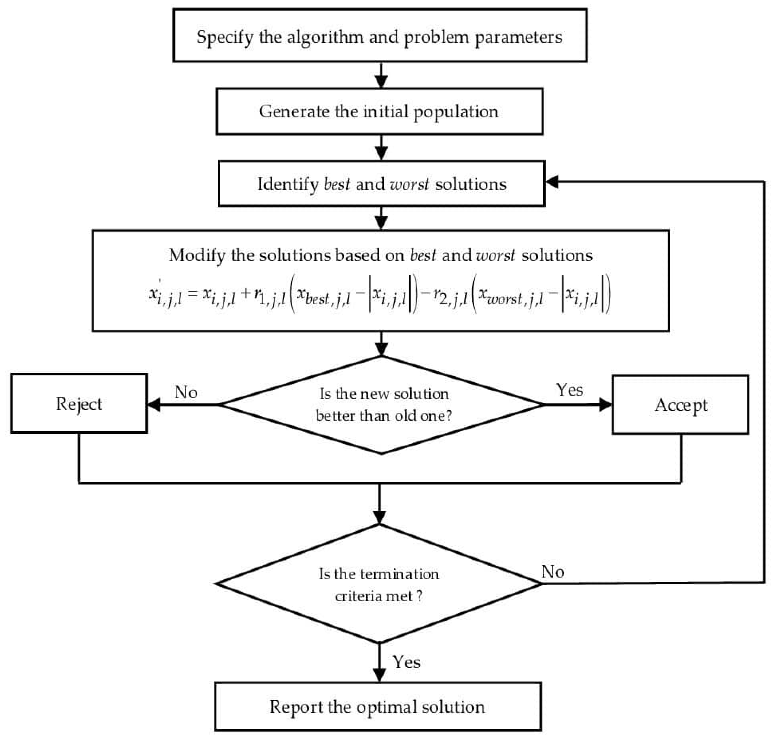
2. The Original Jaya Algorithm

The Jaya algorithm is an optimization technique introduced by Rao. It has been applied for the solution of various unconstrained and constrained optimization problems [33]. In the Jaya algorithm, the searching agents or candidate solutions for a given optimization problem always try to go closer to the best solution by moving away from the worst one. Compared to other computation techniques, this algorithm has the advantages of being simple to implement and easy to understand. Moreover, the Jaya algorithm does not require specific parameters except two common control parameters, namely the maximum function evaluations and the population size.

In the Jaya algorithm, the population consists of a group of candidate solutions and the different variable values represent the decision variables to be optimized. The objective function value is equivalent to the fitness of the optimization problem. In the initialization process, the random variables of the searching agents can be determined with the following equation:

$$x_{i,j}=x_{\min ,j}+(x_{\max ,j}-x_{\min ,j}) \mathrm{rand}(0, 1)$$

(1)

where $x_{i,j}$ is the jth variable of i candidate solution; $x_{\max ,j}$, $x_{\min ,j}$ are the jth variable boundaries ($j=1,2,\dots D$, where D is the number of decision variables) for the $X_i$ candidate solution ($i=1,2,\dots NP$, $NP$ is the population size) and rand(0, 1) is a random number in the range (0, 1).

After initializing the NP candidate solutions $X_i=[x_{i,1},x_{i,2},\dots x_{i,j},\dots x_{i,D}],$ $i=1,2,\dots NP,$ an objective function $F(X_i)=F_i$ is used for evaluating these solutions. The searching agents associated respectively with the best and worst function values (i.e., $F_{best}$ and $F_{worst}$) among the population are designed by best and worst. The whole operating process of the Jaya algorithm can be formulated as follows:

$$x_{i,j,l}^{\prime }=x_{i,j,l}+r_{1,j,l}(x_{best,j,l}-|x_{i,j,l}|)-r_{2,j,l}(x_{worst,j,l}-|x_{i,j,l}|)$$

(2)

where $x_{best,j,l}$ and $x_{worst,j,l}$ are respectively the values of the jth parameter for the best and worst candidates during the lth iteration. $x_{i,j,l}^{\prime }$ is the newly generated value according to $x_{i,j,l}$ and $r_{1,j,l}$ and $r_{2,j,l}$ are two different random numbers within [0, 1]. The term $r_{1,j,l}(x_{best,j,l}-|x_{i,j,l}|)$ indicates the solution tendency to move nearer to the best solution and the term $-r_{2,j,l}(x_{worst,j,l}-|x_{i,j,l}|)$ indicates the solution tendency to shun the worst solution. The new candidate solution $X_i^{\prime }$ is accepted if it provides a better function value than the old solution $X_i$. At the end of each iteration, the accepted function values are maintained and they are considered for the next iteration. The flowchart of the original Jaya algorithm is shown in Figure 1. This algorithm strives to move closer to success (i.e., approaching only the best solutions) and to evade failure (i.e., avoiding all the worst solutions). The algorithm can achieve victory by reaching the best solution and so it is called Jaya (i.e., victory).

3. The Hybrid CJaya-SQP Method

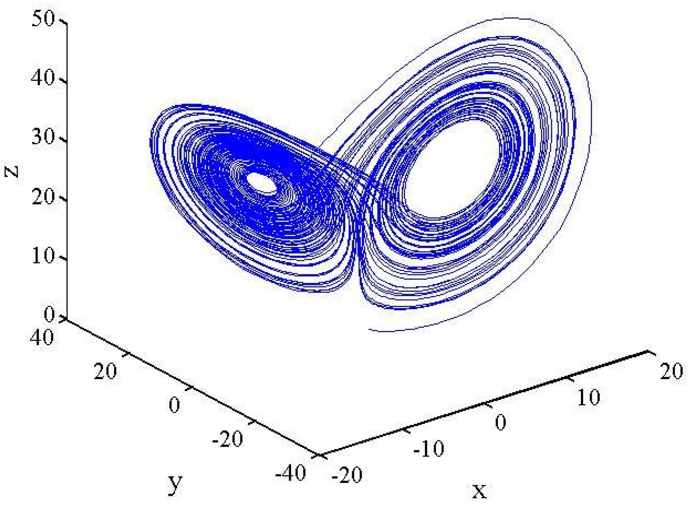
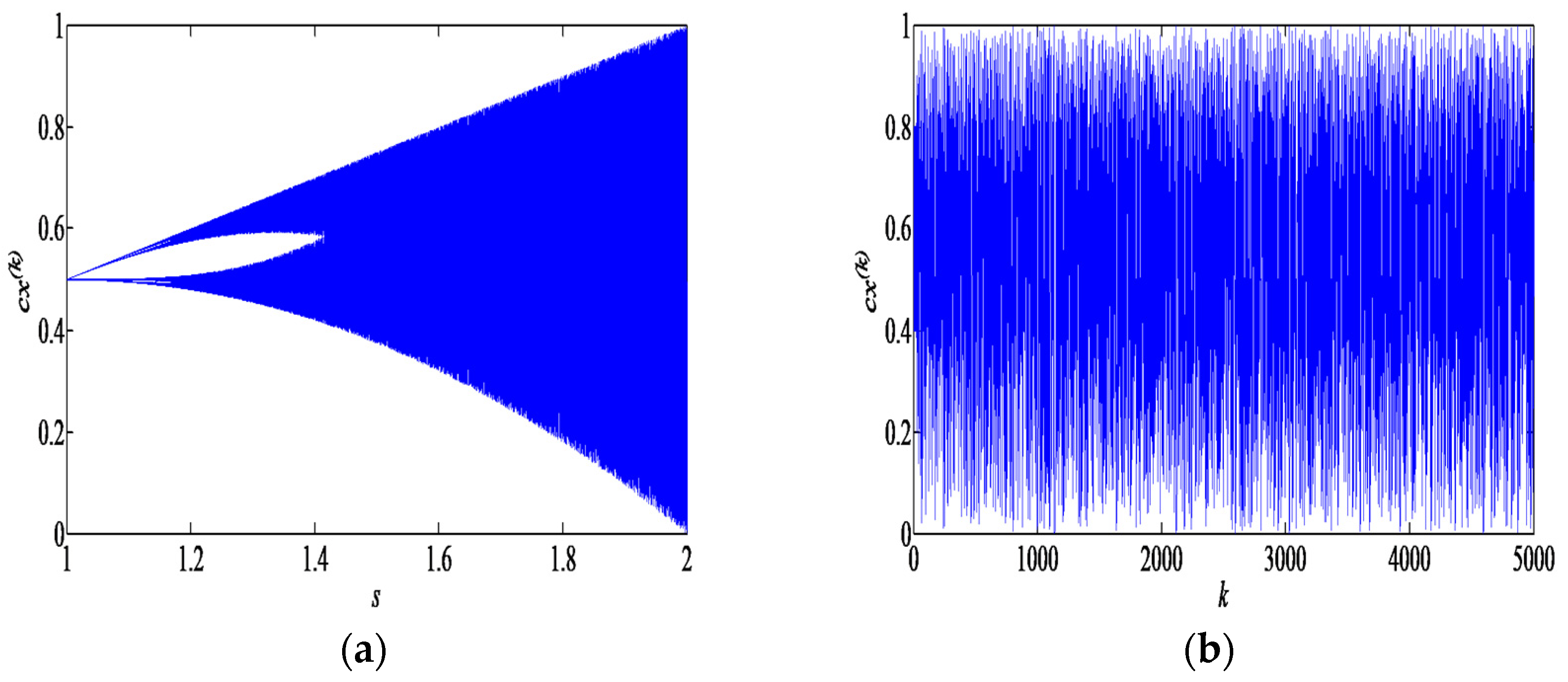
In the Jaya algorithm, the searching agents are updated by moving closer to the best solution and avoiding the worst one, which grants a good diversification and intensification to the search process. However, this algorithm suffers from the problem of slow convergence when the global best solution obtained is around the locally optimal solution. As a result, the premature convergence can be encountered and the Jaya algorithm can easily get stuck on local optimums; furthermore, it is strenuous to achieve the balance between exploitation and exploration. To alleviate this problem, the searching ability and the population diversity of the original Jaya algorithm must be increased. To serve this goal, the chaotic system and the SQP algorithm are introduced into this algorithm. The chaotic map is first employed to improve the uniformity of all random numbers in Jaya. Secondly, a novel chaotic phase is used to enhance the local search behavior of this algorithm. Thirdly, the SQP algorithm is used as a deterministic local search algorithm for finding the local optimistic result.

3.1. Chaotic Map

Chaos has been widely used in optimization problems owing to its easy implementation, dynamic behavior, ergodicity and unpredictability. It has a strong potential in optimization problems for exploring the solution space and getting the global optimum. The combination of optimization algorithms with chaotic maps has been introduced in several works. In this research paper, two chaotic maps, namely Lorenz system and Tent map, are employed to enhance the searching process of the original Jaya algorithm. The Lorenz system is a three-dimensional map defined by the following coupled differential equations:

$$\begin{array}{l}\dot{x}=\sigma (y-x)\\ \dot{y}=x(\rho -z)-y\\ \dot{z}=xy-\beta z\end{array}$$

(3)

where $\dot{x}=dx/dt$, $\dot{y}=dy/dt$, $\dot{z}=dz/dt$ and σ, ρ, β are positive real parameters. For σ = 10, β = 8/3 and ρ = 28, the Lorenz system exhibits a chaotic attractor [54]. The Lorenz attractor is illustrated in Figure 2.

In this work, the $z(t)$ component of Lorenz system is normalized in the range [0, 1] before being applied to the Jaya algorithm according to Equation (4).

$$cz(t)=\frac{z(t)-z_{\min }}{z_{\max }-z_{\min }}$$

(4)

where $z_{\min }$ and $z_{\max }$ indicate respectively the minimum and maximum values of the Lorenz system’s $z(t)$ component and $cz(t)$ represents the normalized chaotic variables in the range [0, 1].

The chaotic Tent map is one of the most typical unimodal maps. It is a piecewise linear map of the interval [0, 1] expressed as follows:

$$c{x}^{(k+1)}=T_s(c{x}^{(k)})=\{\begin{array}{cc}sc{x}^{(k)},& 0\le c{x}^{(k)}<0.5\\ s(1-c{x}^{(k)}),& 0.5\le c{x}^{(k)}\le 1\end{array}$$

(5)

where $c{x}^{(k)}$ denotes the value of the chaotic variable in the kth iteration and $c{x}^{(0)}\notin \left\{1/4,1/2,3/4\right\}$. s is the control parameter restricted to the interval (1, 2]. The Tent map is introduced in this study to the CLS process in order to alleviate the premature convergence. The bifurcation diagram presented in Figure 3a indicates that the Tent map reaches the chaotic behavior when the chaos-parameter-region $s\in \left[\sqrt{2},2\right]$ [55]. This is confirmed by the ergodic property of this chaotic map, shown in Figure 3b, where the initial value is $c{x}^{(0)}=0.4$ and the iterative times is $k=5000$.

3.2. Original Jaya with Chaos

In this work, the Lorenz chaotic attractor is used to generate the initial candidate solutions instead of the random initialization in the original Jaya, with the aim of increasing the initial population’s diversity and the convergence speed. Using the Lorenz system, the initial population is generated as follows:

$$x_{i,j}=x_{\min ,j}+c{z}_{i,j}(x_{\max ,j}-x_{\min ,j})$$

(6)

where $c{z}_{i,j}$ denotes the chaotic variable of the jth parameter for the ith candidate given by the Lorenz system. This way of defining Equation (6) avoids the drawback set by using Equation (1), in which the initial population generated suffers severely from the lack of diversity, which may degrade the convergence property of the Jaya algorithm. Moreover, this procedure provides a higher ability of the population to reach as fast as possible the optimum solution and thus reducing the computational effort regarding the number of function evaluations and the implementation time.

In the original Jaya algorithm, the mechanism of updating the candidate solutions is based on approaching only the best solutions as well as strictly avoiding all of the worst solutions at every iteration. The quality of the searching agents is randomly updated according to the difference between the best solution and the current candidate as well as the worst solution and the current candidate. In the proposed algorithm, the Lorenz system serves to generate chaotic sequences in order to replace the random values used for solution updates in the Jaya algorithm. It is worth noting that using the suggested chaotic mutation to update the candidate solutions can result in the improvement of their quality and stability. The novel formula for updating the solutions can be formulated as follows:

$$x_{i,j,l}^{\prime }=x_{i,j,l}+c{z}_{1i,j,l}(x_{best,j,l}-|x_{i,j,l}|)-c{z}_{2i,j,l}(x_{worst,j,l}-|x_{i,j,l}|)$$

(7)

where $c{z}_{1i,j,l}$ and $c{z}_{2i,j,l}$ are two different chaotic variables generated by Lorenz system for the jth parameter of the ith candidate during the lth iteration. The proposed updating process of the candidate solutions avoids the problem set by using Equation (2) in which the random numbers whose values lie within [0, 1] are unable to ensure optimization ergodicity in the search space. Moreover, the chaotic sequences embedded into the conventional Jaya algorithm to generate the initial solutions and control the search process are able to boost the global search capability of the proposed algorithm and to achieve a good diversification of the searching process.

3.3. Chaotic Local Search Method (CLS)

In this section, a novel CLS method is introduced to help Jaya avoid the premature stagnation in the local optimum and to boost the exploitation ability of the algorithm. In fact, the CLS improves the original Jaya performances regarding the solutions quality, convergence speed propriety and computational effort. In this research, the CLS is applied around the current best candidate solution X_best. The range around X_best can be the best area to proceed to the optimum global solution. The process of the CLS method based on the Tent map is presented as follows:

Step 1: Set $k=1$ and then generate the chaotic variables $c{x}_j^{(1)}$ using Equation (5). k denotes the iteration number of the CLS.

Step 2: Evaluate the target vector $X_{t,i}=(x_{t,i,1},x_{t,i,2},\dots ,x_{t,i,D})$ using the following equation:

$$x_{t,i,j}^{(k)}=x_{best,j}+c{x}_j^{(k)}(x_{best,j}-SF{x}_{avg,j}) j=1,2,\dots ,D$$

(8)

where $X_{avg}$ is the mean value of the candidate solutions represented as follows: $X_{avg}=\frac{1}{NP}\left[{\displaystyle {\sum }_{i=1}^{NP}{x}_{i,1}},{\displaystyle {\sum }_{i=1}^{NP}{x}_{i,2}},\dots ,{\displaystyle {\sum }_{i=1}^{NP}{x}_{i,D}}\right]$ and SF is the scaling factor expressed by $SF=round([1+rand(0,1)\{2-1\}])$. $c{x}_j^{(k)}$ is the jth chaotic variable which ensures the control of the difference vector $(X_{best}-SF\times X_{avg})$ to alter the target vector.

Step 3: Check if the decision variables $x_{t,i,j}^{(k)},j=1,2,\dots ,D$ are still be clamped to the predefined search space $[x_{\min ,j},x_{\max ,j}]$ according to Equation (9):

$$x_{t,i,j}^{(k)}=\max \left\{\min \left\{x_{t,i,j}^{(k)},x_{\max ,j}\right\},x_{\min ,j}\right\}$$

(9)

Step 4: Evaluate the decision variables $x_{t,i,j}^{(k)},j=1,2,\dots ,D$. If $X_{t,i}^{(k)}$ is better than $X_i$ in terms of the objective function value, go to the next step. Otherwise, go to step 6.

Step 5: Set $x_{i,j}=x_{t,i,j}^{(k)}$$(j=1,2,\dots ,D)$ and stop the CLS method.

Step 6: Set $k=k+1$, if the iteration time $k\le k_{\max }$, where $k_{\max }$ denotes the maximum iteration number of the CLS, evaluate the chaotic variables $c{x}_j^{(k+1)}$ for the next iteration using the Tent equation and turn to step 2.

Based on the proposed Jaya with the Lorenz attractor and the suggested CLS scheme, a novel two-phased iterative strategy called Chaotic Jaya (CJaya) is introduced in this paper. In this algorithm, the original Jaya algorithm combined with the Lorenz system serves as a global search algorithm to provide a global optimistic result, whereas the CLS method is used to ensure the locally oriented search for the solutions obtained by Jaya.

3.4. Sequential Quadratic Programming (SQP)

The SQP is a nonlinear programming algorithm for handling constrained optimization problems [46]. It is the most efficient among all other nonlinear programming techniques regarding solution accuracy, efficiency and success ratios over a wide range of test problems [47]. In the SQP algorithm, the original problem is replaced by a sequence of quadratic programming (QP) sub-problems. This is achieved by linearizing the problem constraints and approximating the Lagrangian function quadratically as follows:

$$L(x,\lambda )=J(x)+{\displaystyle \sum _{i=1}^m{\lambda }_i{G}_i(x)}$$

(10)

where $J(x)$ is the objective function, $G_i(x)$ represents the problem constraints, ${\lambda }_i$ are the Lagrange multipliers and m denotes the total number of constraints.

At each iteration k, the Hessian matrix of the Lagrangian function, $H_k$, is calculated approximately using the quasi-Newton methods [25]. The QP sub-problem is then generated as follows:

$$\begin{array}{l}\min \left(\nabla J{(x_k)}^T{d}_k+\frac{1}{2}{d}_k^T{H}_k{d}_k\right)\\ \mathrm{s}.\mathrm{t}.\{\begin{array}{cc}{G}_i(x_k)+{\left[\nabla G_i(x_k)\right]}^T{d}_k=0& i=1,\dots ,m_e\\ G_i(x_k)+{\left[\nabla G_i(x_k)\right]}^T{d}_k\le 0& i=m_e+1,\dots ,m\end{array}\end{array}$$

(11)

where $d_k$ and $x_k$ are respectively the search direction and the decision vectors at iteration k and $m_e$ represents the number of equality constraints. The QP sub-problem solution is solved to calculate the direction $d_k$ in order to update the control variables and to construct the next iterate as follows:

$$x_{k+1}=x_k+{\alpha }_k{d}_k$$

(12)

The step length value ${\alpha }_k$ is adjusted in such a way as to achieve a sufficient reduction in the merit function.

In summary, the SQP algorithm involves three major stages:

• Update the Hessian of the Lagrangian function;
• Solve the QP sub-problem;
• Calculate a line search and merit function.

The MATLAB optimization toolbox developed by MathWorks (Natick, MA, USA) is used to perform the SQP simulations throughout this study.

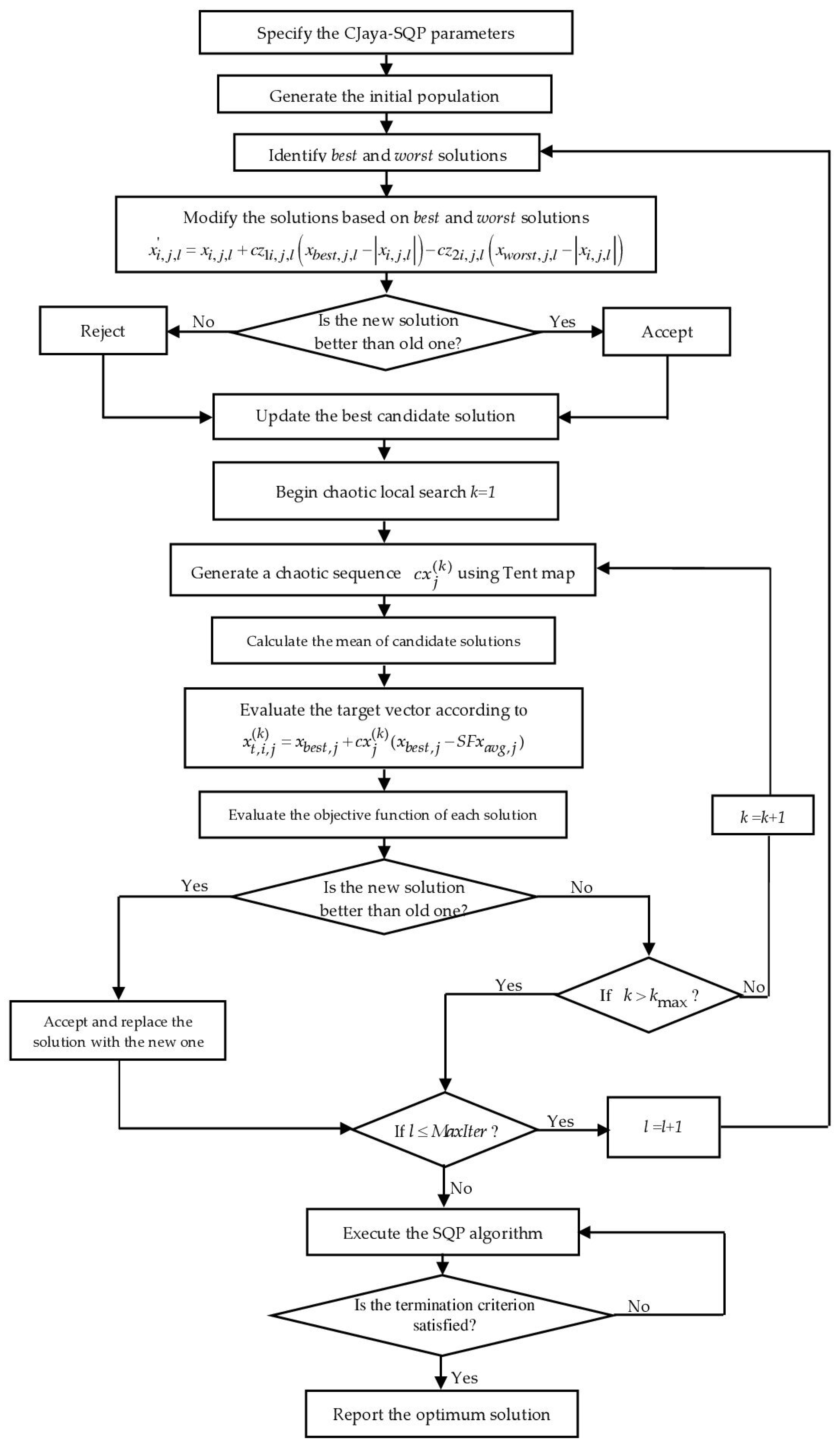
3.5. Hybrid CJaya-SQP Method

By combining the proposed CJaya with the SQP method, a new hybrid algorithm, namely CJaya-SQP, is developed in this paper. The CJaya-SQP’ searching process begins by initializing a group of candidate solutions based on the Lorenz system. Firstly, the CJaya is applied to extract the best candidate in the solution space at every iteration. Secondly, the global best candidate solution is taken as the initial condition for the SQP method, which serves as a local optimizer for searching around the best country explored by the CJaya algorithm. Thereby, the exploitation and exploration abilities can be boosted and the hybrid algorithm can quickly and accurately find the global optimum solution. The flowchart of the proposed CJaya-SQP algorithm is provided in Figure 4.

The detailed procedure of the proposed CJaya-SQP algorithm is described in Algorithm 1. It can be observed that CJaya-SQP is as simple to implement as that of original Jaya and there is no need for any additional control parameter. Given the possibility to strengthen the Jaya algorithm performance by introducing the chaotic system and SQP method to increase the searching process, the CJaya-SQP can have a good performance regarding the optimum solutions’ quality and accuracy.

Algorithm 1: The procedure of CJaya-SQP algorithm.

1: Set the number of design variables (D), population size (NP), maximum function evaluations (MaxFEs), the maximum iteration number $MaxIter=MaxFEs/NP$ and the maximum search length of CLS $k_{\max }$; 2: Initialize: the iteration count l (l = 1), the initial conditions $c{x}_0,c{y}_0,c{z}_0$ for the Lorenz system and $c{x}_0$ for the Tent map; 3: Initialize the NP candidate solutions $\left(X_i, i=1,2,\dots NP\right)$ chaotically within their search boundaries using Equation (6); 4: Calculate the value of the objective functions $F_i=F(X_i)$ of the initial solutions $\left(X_i, i=1,2,\dots NP\right)$ during iteration $l=1$; 5: Repeat     6: Identify the indexes assigned to the best candidate $X_{best}$, $best=Arg(Min(F_i, i=1,2,\dots NP))$ and the worst candidate $X_{worst}$, $worst=Arg(Max(F_i, i=1,2,\dots NP))$ and evaluate $F_{best}=F(X_{best})$ and $F_{worst}=F(X_{worst})$;     7: For $i=1$ To NP Do         8: Produce the new solution $X_i^{\prime }$ by updating the $x_{i,j}$ variables for the $X_i$ candidate solution using Equation (7);         9: Check the variables’ boundaries;            {Compare the new solution $X_i^{\prime }$ with the old one $X_i$};         10: If $F(X_i^{\prime })<F(X_i)$ Then $X_i=X_i^{\prime }$, $F(X_i)=F(X_i^{\prime })$            End If         End For        {Update the best candidate solution Xbest and its function value Fbest = F(Xbest) };     11: For $i=1$ To NP Do         12: Initialize the iteration count of the CLS k (k = 1);         13: Repeat              14: Generate the chaotic variables $c{x}_j^{(k)}$ for the Tent map using Equation (5);              15: Evaluate the $x_{t,i,j}$ components of the target vector Xt,i using Equation (8);              16: Check if the design variables are in the search space using Equation (9);              {Compare the target vector $X_{t,i}$ with the candidate solution $X_i$};              17: If $F(X_{t,i})<F(X_i)$ Then $X_i=X_{t,i}$, $F(X_i)=F(X_{t,i})$, $k=k_{\max }$               End If              18: $k=k+1$; {increment the iteration count of the CLS}        19: Until $k\le k_{\max }$ (End Repeat)        {Update the best solution Xbest and the function value Fbest = F(Xbest) };        20: If $F(X_i)<F(X_{best})$ Then $X_{best}=X_i$, $F_{best}=F(X_i)$             End If        End For 21: $l=l+1$ {increment the iteration count} 22: Until $l\le MaxIter$ (End Repeat) 23: Let the best solution $X_{best}$ extracted by CJaya be the initial condition for SQP; 24: Use the SQP method for searching around $X_{best}$ which is derived by CJaya; 25: Output the global optimum solution found by SQP.

4. Problem Statement

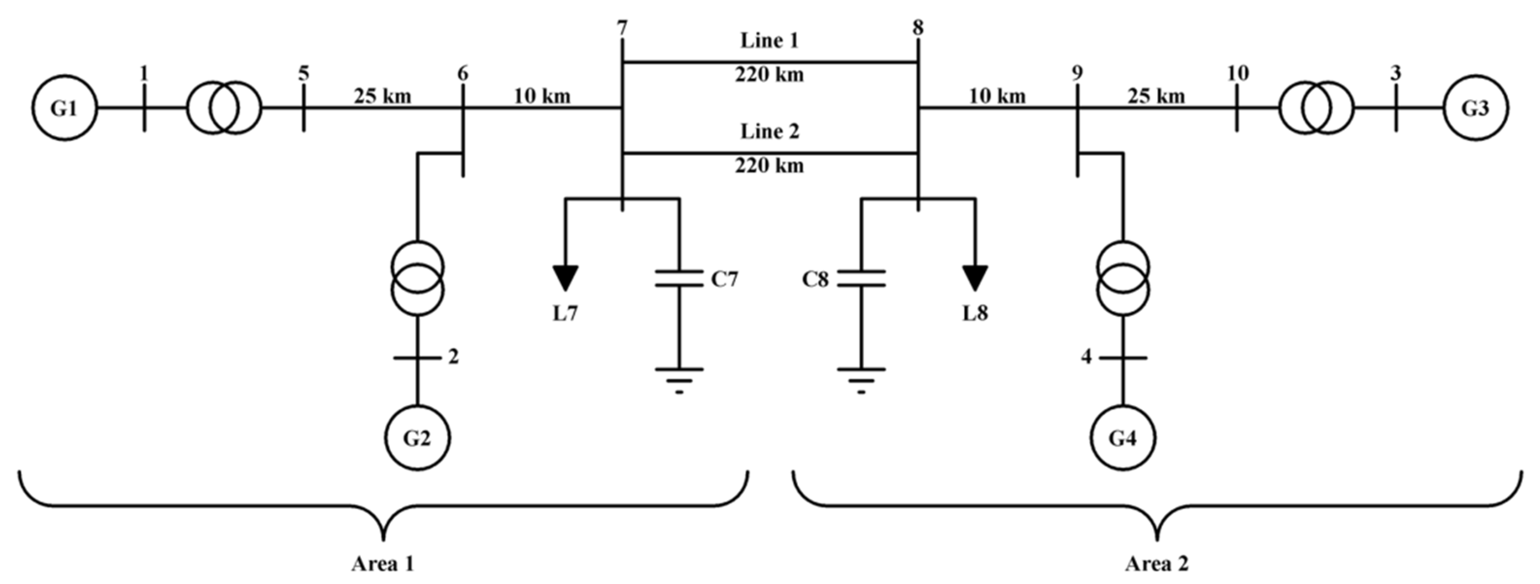
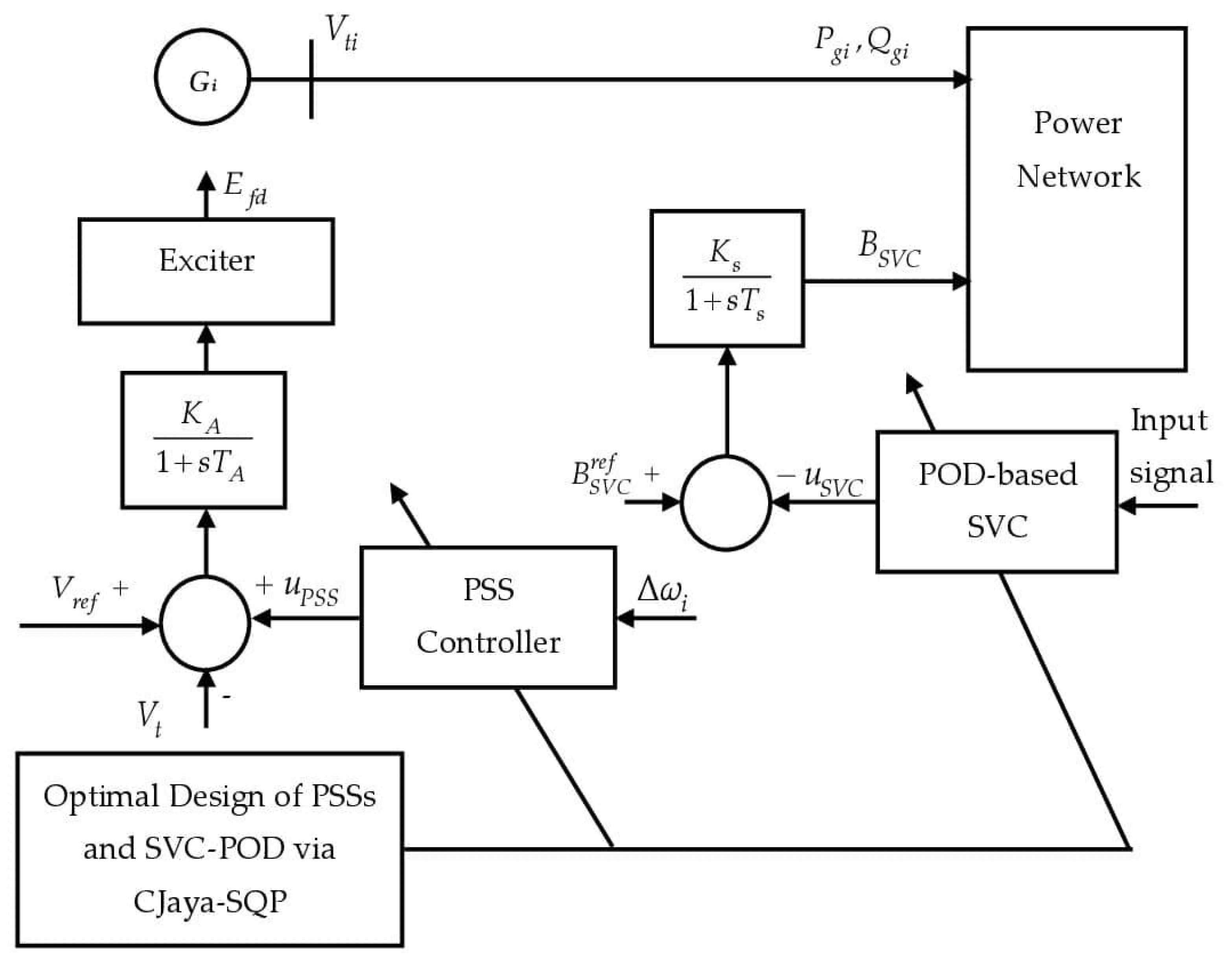
4.1. Power System Model

The power system equipped with PSSs and SVC damping controllers is shown in Figure 5. In this research paper, the optimal tuning of the controllers parameters is achieved by applying the proposed CJaya-SQP method. For clarity, the different variables involved in the power system modeling, including synchronous machines, excitation system, PSSs and SVC controllers are given in

Table 2. List of variables.

Symbol	Variable Description	Symbol	Variable Description
$E_q^{\prime },E_{fd}$	Internal and the field voltages, respectively.	$B_{SVC}$	SVC susceptance.
$\delta ,\omega$	Rotor angle and speed, respectively.	$B_{SVC}^{ref}$	Reference susceptance of SVC.
$V_{ref},V_t$	Reference and terminal voltages, respectively.	$N$	Total number of buses.
$u_{PSS},u_{SVC}$	PSS and SVC stabilizing signals, respectively.	$N_L$	Total number of load buses.
$K_{PSS}$	Gain of the PSS.	$P_s$	Real power injected at the slack bus s.
$T_{wp}$	Washout time constant of PSS.	$P_{gs}$	Real power generation at the slack bus s.
$T_{1p}-T_{4p}$	Lead-lag time constants of PSS.	$P_{ds}$	Real power demand at the slack bus s.
$\Delta {\omega }_i$	Change in speed for machine i.	$V_s\angle {\alpha }_s,V_j\angle {\alpha }_j$	Voltages at the end buses s and j.
$K_A,T_A$	Gain and time constant of the excitation system, respectively.	$Y_{sj}\angle {\theta }_{sj}$	$\mathrm{The} \left(s,j\right)\mathrm{th}$ element of the power system admittance matrix.
$K_s,T_s$	SVC gain and time constant, respectively.	$P_D$	Total real power demand.
$K_{SVC}$	Gain of lead-lag circuits of SVC.	$P_{Loss}$	Real power loss.
$T_{ws}$	Washout time constant of SVC.	$P_{gi},Q_{gi}$	Real and reactive powers generated by machine i.
$T_{1s}-T_{4s}$	Lead-lag time constants of SVC.

.

The power system model can be formulated by a nonlinear set of coupled differential equations as follows:

$$\dot{x}=f\left(x,u\right)$$

(13)

where $x={[\delta ,\omega ,E_q^{\prime },E_{fd}]}^T$ and $u={\left[u_{PSS},u_{SVC}\right]}^T$ are the state and the control vectors, respectively.

In this study, the coordination between both controllers is achieved through linearization of Equation (13) around an operating condition. The linearized model of a power network with $n$ machines, $m$ PSSs and SVC is described as follows:

$$\dot{x}=Ax+Bu$$

(14)

where $A$ is a $4n\times 4n$ matrix and equals $\partial f/\partial x$ while $B$ is a $4n\times m$ matrix and equals $\partial f/\partial u$. x is a $4n\times 1$ state vector and $u$ is an $m\times 1$ input vector.

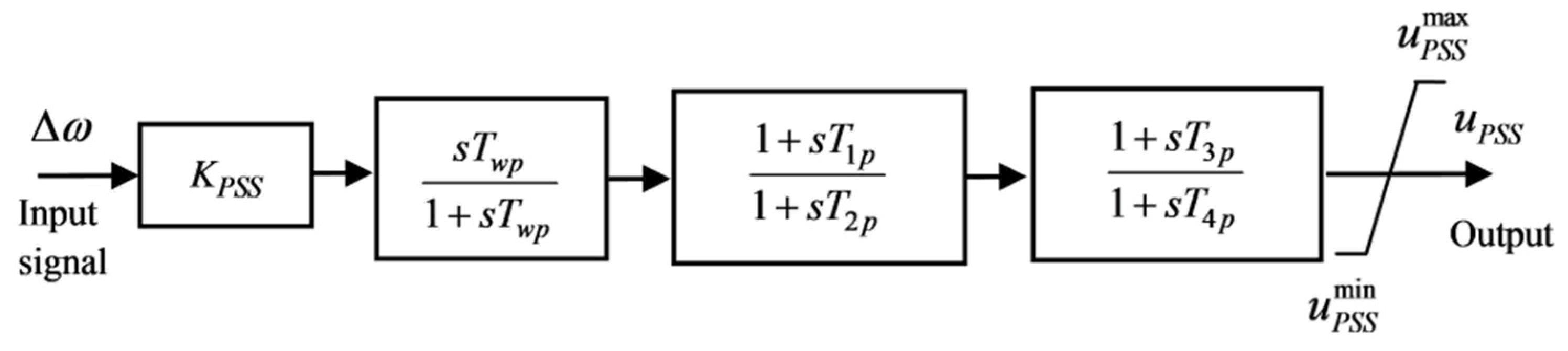
4.2. PSS Modeling and Damping Controller Structure

A PSS is a complementary controller in the excitation system of the machine. It is used to mitigate rotor oscillations. To serve this goal, the PSS produces a proper torque on the machine rotor in order to compensate the phase lag between the generator electrical torque and the excitation voltage. The conventional PSS (CPSS) shown in Figure 6 is adopted throughout this study. The choice of this type of stabilizer is made with regard to its flexibility, simplicity and ease of implementation and online tuning. It comprises a washout filter whose time constant $T_{wp}$ is in the range of 0.5–20 s [8] and a lead-lag compensator.

The dynamic compensator of the suggested PSS comprises two lead-lag blocks with time constants $T_{1p}-T_{4p}$, a complementary gain $K_{PSS}$ and a limiter. The lead-lag blocks are considered to provide the convenient phase-lead to mitigate the phase lag between the electrical torque of the machine and the excitation voltage.

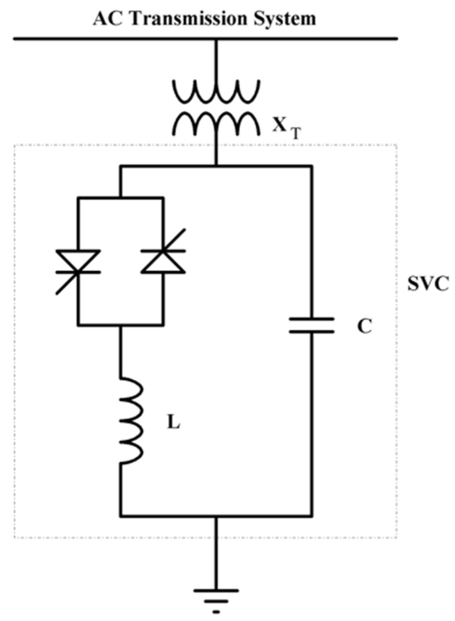
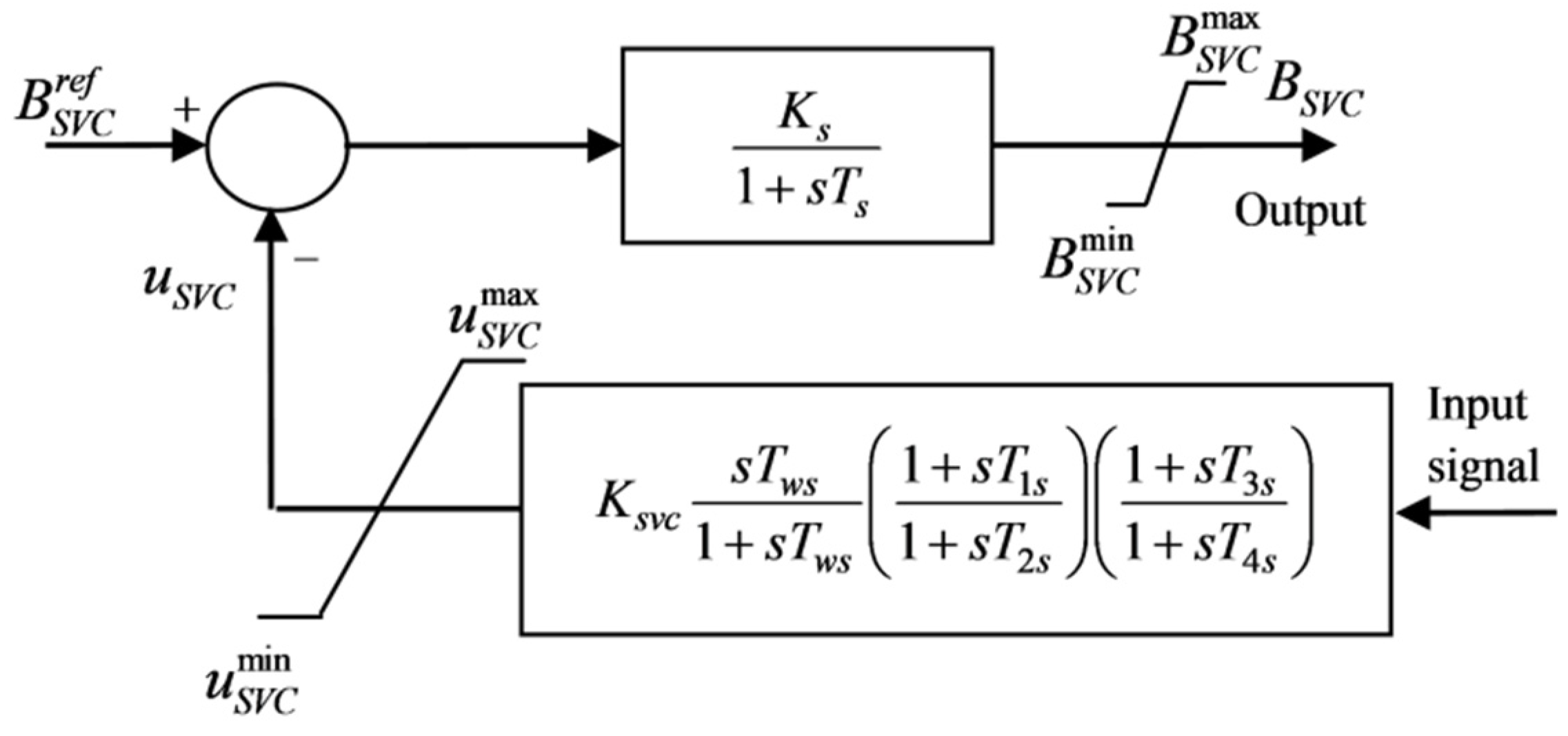
4.3. SVC Modeling and Damping Controller Structure

The SVC device used in this study is connected to the AC system via a set up transformer to keep the network voltage constantly at a set reference value by varying its effective susceptance. As shown in Figure 7, the system is a thyristor-controlled reactor/fixed capacitor (TCR/FC). The effective susceptance of an SVC is controlled by the firing angle $\alpha$ of the thyristors that varies between 90° and 180°.

For dynamic stability studies, the SVC is considered as a variable susceptance. The dynamic equation of the SVC susceptance can be written as follows:

$${\dot{B}}_{SVC}=\frac{1}{T_s}\left(K_s\left(B_{SVC}^{ref}-u_{SVC}\right)-B_{SVC}\right)$$

(15)

where $B_{SVC}^{ref}$ is the reference susceptance of the SVC. $K_s$ and $T_s$ are the SVC gain and time constant, respectively. The SVC can be used to enhance the damping of EMOs by adding an auxiliary stabilizing signal in its control system. As depicted in Figure 8, the structure of the proposed SVC with a lead-lag compensator is composed of a gain block $K_{SVC}$, a washout block with the time constant $T_{ws}$ and two stage phase-compensation blocks with the time constants $T_{1s}-T_{4s}$ and a limiter.

Many input signals are suggested for the FACTS-based damping controllers in order to provide electric power with an adequate damping, especially for the inter-area oscillations. In this regard, the selection of the appropriate input signal of the damping controllers to achieve the best performance is an important issue. The rotor speed deviation has been frequently suggested as an effective input signal in several studies [19]. For this reason, the speed deviation is adopted as the input signal of SVC in this study. The adjustable parameters of the PSSs and SVC damping controllers for the purpose of coordinated design are selected using the proposed hybrid CJaya-SQP algorithm.

4.4. Optimal SVC Location Method

Mostly, SVC controllers are installed in electric power systems in order to ameliorate the voltage profile and to minimize the system losses. Thus, total RPL can be considered as a determinant parameter for the SVC location. For optimum location of the SVC, a new RPL sensitivity-based method is proposed in this paper.

In the decoupled load flow modal, the incremental bus voltage magnitude is given as follows [56]:

$$\Delta V=J_{qv}^{-1}\Delta Q$$

(16)

where $\Delta Q$ denotes the reactive power mismatch vector between the calculated values and the specified values and $J_{qv}$ is the Jacobian matrix, which involves the partial derivatives of the reactive power injections with respect to the bus voltage magnitudes. The active power injected at the swing bus s is expressed as follows:

$$P_s=P_{gs}-P_{ds}=V_s{\displaystyle \sum _{j=1}^N{Y}_{sj}{V}_j\cos ({\alpha }_s-{\alpha }_j-{\theta }_{sj})}$$

(17)

where $N$ is the total number of buses; $P_{gs}$ and $P_{ds}$ are the active power generation and the real power demand at the slack bus, respectively. $V_s\angle {\alpha }_s$ and $V_j\angle {\alpha }_j$ are respectively the voltages at the end buses s and j; $Y_{sj}\angle {\theta }_{sj}$ is the $\left(s,j\right)\mathrm{th}$ element of the power system admittance matrix.

Moreover, the injected power at the swing bus s can be given by the following equation:

$$P_s=P_D+P_{Loss}-P_{ds}-{\displaystyle \sum _{i=1}^{N-1}{P}_{gi}}$$

(18)

where $P_D$ denotes the total real power demand. $P_{Loss}$ is the active power loss and $P_{gi}$ is the real power generated by machine i. Hence, by substituting $P_s$ from Equation (17) in Equation (18), the total system loss $P_{Loss}$ becomes as follows:

$$P_{Loss}=(-P_D+P_{ds}+{\displaystyle \sum _{i=1}^{N-1}{P}_{gi}})+V_s{\displaystyle \sum _{j=1}^N{Y}_{sj}{V}_j\cos ({\alpha }_s-{\alpha }_j-{\theta }_{sj})}$$

(19)

The sensitivity vector of the total system RPL with respect to the magnitude of injected voltage $V_j$ can be calculated as:

$$\frac{\Delta P_{Loss}}{\Delta V_j}=V_s{\displaystyle \sum _{j=1}^N{Y}_{sj}\cos ({\alpha }_s-{\alpha }_j-{\theta }_{sj})}$$

(20)

where $\Delta P_{Loss}$ is the variation of RPL when the reactive power injected at the jth bus is changed. Because the voltage magnitudes in the PV buses are kept in their specified values, there are only changes in the voltage modules in the PQ buses. By substituting $\Delta V$ from Equation (16) in Equation (20), the total RPL sensitivity vector with respect to the reactive power injections is given as follows:

$$\frac{\Delta P_{Loss}}{\Delta Q_k}={\displaystyle \sum _{k=1}^{N_L}\left({\displaystyle \sum _{j=1}^{N_L}{V}_s{Y}_{sj}}\cos ({\alpha }_s-{\alpha }_j-{\theta }_{sj})J_{qv}^{-1}(j,k)\right)}$$

(21)

where $N_L$ is the total number of load buses. The Equation (21) can be written as follows:

$$\Delta P_{Loss}={\displaystyle \sum _{k=1}^{N_L}{R}_k\Delta Q_k}$$

(22)

where $R_k$ is the sensitivity index introduced as:

$$R_k=V_s{\displaystyle \sum _{j=1}^{N_L}{Y}_{sj}}\cos ({\alpha }_s-{\alpha }_j-{\theta }_{sj})J_{qv}^{-1}(j,k)$$

(23)

Hence, the problem of optimally allocating the SVC device in networks can be solved by a new method based on the total system RPL sensitivity vector.

Criteria for SVC optimal placement

The criteria followed to determine the optimum location of SVC in power networks is as follows:

• The sensitivity factor $R_k=\frac{\partial P_{Loss}}{\partial Q_k}$ which involves changes in RPL with respect to the change in the injection of reactive power is computed for all load buses. The bus having the largest absolute value of the sensitivity is considered as the best location for connecting an SVC controller;
• The SVC device should not be installed in the transmission lines containing the generation buses and transformers, even if the sensitivity factor is the largest there. Indeed, all generators are generally equipped with a PSS whose the main function consists in improving power system stability by producing a supplementary stabilizing signal through the excitation system. Moreover, the SVC device should not be placed in buses where there is no injected power.

5. Coordinated Design of PSSs and SVC via Hybrid CJaya-SQP

To provide the power system with a greater damping and improve its dynamic stability, the PSSs and SVC parameters may be adjusted to minimize simultaneously the two eigenvalue-based objective functions J₁ and J₂ described by Equations (24) and (25). This will provide some degree of relative stability and limits the maximum overshoot of the system.

$$J_1={\displaystyle \sum _{{\sigma }_i\ge {\sigma }_0}{({\sigma }_0-{\sigma }_i)}^2}$$

(24)

$$J_2={\displaystyle \sum _{{\xi }_i\le {\xi }_0}{({\xi }_0-{\xi }_i)}^2}$$

(25)

where ${\sigma }_i$ and ${\xi }_i$ are the real parts and damping ratio of the ith eigenvalue, respectively. Moreover, ${\sigma }_0$ and ${\xi }_0$ are chosen as thresholds. Based on the objective functions, the stabilizers are designed to shift the system-closed loop modes to the D-shape sector, which is characterized by ${\sigma }_i\le {\sigma }_0$ and ${\xi }_i\ge {\xi }_0$ as shown in Figure 9. It is noteworthy that in this study, the most critical oscillation modes which mainly belong to the electromechanical ones are relocated.

In this study, J₁ and J₂ are combined into a single objective function J, defined as follows:

$$J=J_1+\alpha J_2={\displaystyle \sum _{{\sigma }_i\ge {\sigma }_0}{({\sigma }_0-{\sigma }_i)}^2}+\alpha {\displaystyle \sum _{{\xi }_i\le {\xi }_0}{({\xi }_0-{\xi }_i)}^2}$$

(26)

where $\alpha$ is a weighting factor used to simultaneously correlate the abovementioned two objectives with the two functions J₁ and J₂. Its value is derived from various small signal and dynamic stability analyses conducted on the studied power system.

The optimum sizing of PSSs and SVC controllers is considered as a continuous constrained optimization problem whose decision variables are real-valued. As given in Equation (27), the problem-bound constraints are the upper and lower limits of the controllers’ parameters whose values are given in

Table 3. Upper and lower limits of PSSs and SVC parameters.

Case		Lower Limit	Upper Limit
PSS	KPSS	1	100
	Ti (i = 1,2,3,4)	0.001	2
SVC	Ksvc	1	150
	Ti (i = 1,2,3,4)	0.001	2

.

$$\{\begin{array}{c}{K}_{PSS,\min }\le K_{PSS}\le K_{PSS,\max }\\ K_{svc,\min }\le K_{svc}\le K_{svc,\max }\\ T_{i,\min }\le T_i\le T_{i,\max }\end{array}$$

(27)

In the light of the discussion presented above, the challenge of the coordination design between the SVC-based damping controller and PSSs parameters lies in the improvement of the system’s overall dynamic stability. This is achieved by applying the proposed hybrid CJaya-SQP algorithm as an optimization technique. The decision variables to be optimized by the proposed approach are the PSS and SVC parameters. It consists of the PSS gain K_PSS, the time constants of the lead-lag blocks T_1p–T_4p, the SVC gain K_svc and the lead-lag time constants T_1s–T_4s. In this research study, there are 10 bound constraints and 20 parameters to be optimized, which are selected as continuous decision variables. It is worth mentioning that the initial values of controllers’ parameters are chaotically generated using the Lorenz system within their search boundaries using Equation (6). The washout time constants for both PSS and SVC are kept fixed during the design process. In this study, $T_{wp}=T_{ws}=10 \mathrm{s}$ is used. The flowchart of the proposed simultaneous coordination design of the PSSs and SVC damping controllers by the proposed hybrid CJaya-SQP algorithm is provided in Figure 10.

6. Numerical Experiments

6.1. Benchmark Functions and Parameter Settings

In order to evaluate the proposed CJaya-SQP algorithm, it is used for minimizing a set of 17 benchmark functions. These functions are frequently applied to test the robustness and efficiency of computing techniques. The choice of these functions is made regarding their different types, including continuous, discontinuous, regular, irregular, unimodal, multimodal, separable, non-separable and multidimensional. The performance of the developed CJaya-SQP is compared to the original Jaya and another five optimization techniques, namely DE, PSO, ABC, IWO and FA.

A function is called unimodal if it has a single global optimum, whereas if it has many local optimums it will be named multimodal. The multimodal functions are employed to assess the ability of a given algorithm to move away from local minima. Hence, an algorithm with a poor exploration is not able to discover efficiently the whole space, and therefore it may be trapped in local minima. A separable function can be described by the sum of functions of one variable. The non-separable functions present an interrelationship between their variables which makes them more difficult compared to the separable functions. In addition, a regular function is differentiable at each point in its domain.

Table 4. Benchmark functions considered in experiments.

Function	Formula	Range	T-Value
	Category I: Conventional problems
Sphere	$f_1(x)={\displaystyle {\sum }_{i=1}^D{x}_i^2}$	[−100, 100]	1 × 10−2
Schwefel 1.2	$f_2(x)={{\displaystyle {\sum }_{i=1}^D\left({\displaystyle {\sum }_{j=1}^i{x}_j}\right)}}^2$	[−100, 100]	1 × 10−5
Schwefel 2.22	$f_3(x)={\displaystyle {\sum }_{i=1}^D|x_i|}+{\displaystyle {\prod }_{i=1}^D|x_i|}$	[−10, 10]	1 × 10−5
Zakharov	$f_4(x)={{\displaystyle {\sum }_{i=1}^D{x}_i^2+\left({\displaystyle {\sum }_{i=1}^{D}0.5i{x}_i}\right)}}^2+{\left({\displaystyle {\sum }_{i=1}^{D}0.5i{x}_i}\right)}^4$	[−5, 10]	1 × 10−5
Rosenbrock	$f_5(x)={\displaystyle {\sum }_{i=1}^{D-1}\left[100{\left(x_{i+1}-x_i^2\right)}^2+{\left(x_i-1\right)}^2\right]}$	[−2.048, 2.048]	5
Rastrigin	$f_6(x)={\displaystyle {\sum }_{i=1}^D[x_i^2-10\cos (2\pi x_i)+10]}$	[−5.12, 5.12]	1 × 10−5
Salomon	$f_7(x)=1-\cos \left(2\pi \sqrt{{\displaystyle {\sum }_{i=1}^D{x}_i^2}}\right)+0.1\sqrt{{\displaystyle {\sum }_{i=1}^D{x}_i^2}}$	[−100, 100]	1 × 10−5
Ackley	$f_8(x)=-20\exp \left(-0.2\sqrt{\frac{1}{D}{\displaystyle {\sum }_{i=1}^D{x}_i^2}}\right)-\exp \left(\frac{1}{D}{\displaystyle {\sum }_{i=1}^D\cos \left(2\pi x_i\right)}\right)+20+e$	[−32.768, 32.768]	1 × 10−5
Griewank	$f_9(x)={\displaystyle {\sum }_{i=1}^D\frac{x_i^2}{4000}}-{\displaystyle {\prod }_{i=1}^D\cos \left(\frac{x_i}{\sqrt{i}}\right)}+1$	[−600, 600]	1 × 10−5
	Category II: Rotated problems
Rotated Schwefel 1.2	$f_{10}(x)=\begin{array}{cc}{{\displaystyle {\sum }_{i=1}^D\left({\displaystyle {\sum }_{j=1}^i{y}_j}\right)}}^2& y=M\times x\end{array}$	[−100, 100]	1 × 10−5
Rotated Schwefel 2.22	$f_{11}(x)=\begin{array}{cc}{\displaystyle {\sum }_{i=1}^D|y_i|}+{\displaystyle {\prod }_{i=1}^D|y_i|}& y=M\times x\end{array}$	[−10, 10]	1 × 10−5
Rotated Zakharov	$f_{12}(x)=\begin{array}{cc}{{\displaystyle {\sum }_{i=1}^D{y}_i^2+\left({\displaystyle {\sum }_{i=1}^{D}0.5i{y}_i}\right)}}^2+{\left({\displaystyle {\sum }_{i=1}^{D}0.5i{y}_i}\right)}^4& y=M\times x\end{array}$	[−5, 10]	1 × 10−5
Rotated Rosenbrock	$f_{13}(x)=\begin{array}{cc}{\displaystyle {\sum }_{i=1}^{D-1}\left[100{(y_{i+1}-y_i^2)}^2+{(y_i-1)}^2\right]}& y=M\times x\end{array}$	[−2.048, 2.048]	50
Rotated Rastrigin	$f_{14}(x)=\begin{array}{cc}{\displaystyle {\sum }_{i=1}^D[y_i^2-10\cos (2\pi y_i)+10]}& y=M\times x\end{array}$	[−5.12, 5.12]	1 × 10−5
Rotated Salomon	$f_{15}(x)=\begin{array}{cc}1-\cos \left(2\pi \sqrt{{\displaystyle {\sum }_{i=1}^D{y}_i^2}}\right)+0.1\sqrt{{\displaystyle {\sum }_{i=1}^D{y}_i^2}}& y=M\times x\end{array}$	[−100, 100]	1 × 10−5
Rotated Ackley	$f_{16}(x)=\begin{array}{cc}-20\exp \left(-0.2\sqrt{\frac{1}{D}{\displaystyle {\sum }_{i=1}^D{y}_i^2}}\right)-\exp \left(\frac{1}{D}{\displaystyle {\sum }_{i=1}^D\cos \left(2\pi y_i\right)}\right)+20+e& y=M\times x\end{array}$	[−32.768, 32.768]	1 × 10−5
Rotated Griewank	$f_{17}(x)=\begin{array}{cc}{\displaystyle {\sum }_{i=1}^D\frac{y_i^2}{4000}}-{\displaystyle {\prod }_{i=1}^D\cos \left(\frac{y_i}{\sqrt{i}}\right)}+1& y=M\times x\end{array}$	[−600, 600]	1 × 10−5

presents the formula, the decision variables’ boundaries of the chosen benchmark functions as well as the T-Values which correspond to the maximum values for accepting the obtained solutions. The global minimum value of all these functions is zero. Experiments are performed for both 30- and 100-dimensional benchmark problems.

All benchmark functions are solved using both the developed CJaya-SQP algorithm and six other optimization algorithms, including the original Jaya, DE, PSO, ABC, IWO and FA. These functions can be grouped as conventional and rotated problems. The conventional problems are classified into unimodal (f₁–f₅) and multimodal (f₆–f₉) functions, whereas the rotated problems (f₁₀–f₁₇) are the rotated versions of f₂–f₉. The latter type of problem is more complex than conventional test functions. For minimizing the statistical errors, the results including the mean, the standard deviation (SD) and the standard error of means (SEM) of each test function for the seven algorithms are obtained for 30 independent runs. All the simulation experiments in this paper are performed on an Intel (R) Core (TM) i7-5500 U CPU 2.40 GHz personal computer and programs are implemented using a Matlab R2014a environment. For a fair comparison, all common parameters of the studied algorithms have the same values. In this study, the population size is 40 and the number of function evaluations (FEs) is 80,000.

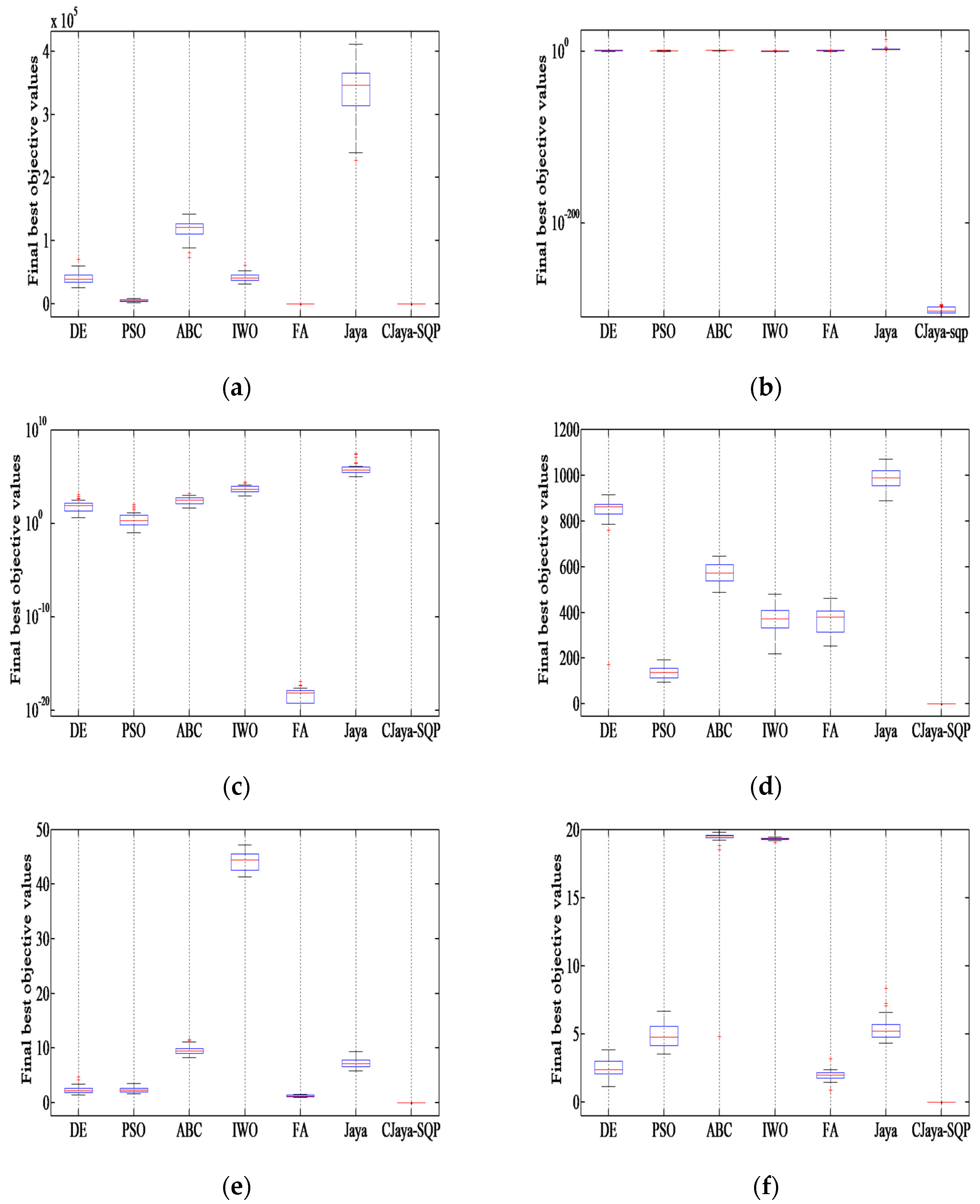
6.2. Results for Low-Dimensional Problems

6.2.1. Comparison of Solution Accuracy

From the results presented in

Table 5. Statistical results obtained by comparative algorithms for 30-dimensional functions over 30 runs with 80,000 function evaluations.

Function		DE	PSO	ABC	IWO	FA	Jaya	CJaya-SQP
f1	Mean	1.78 × 10−29	8.32 × 10−39	5.67 × 10−16	3.29 × 10−5	4.72 × 10−34	2.45 × 10−10	0.00
	SD	1.87 × 10−29	1.55 × 10−38	1.01 × 10−16	4.95 × 10−6	5.85 × 10−35	1.75 × 10−10	0.00
	SEM	3.42 × 10−30	2.83 × 10−39	1.85 × 10−17	9.04 × 10−7	1.06 × 10−35	3.20 × 10−11	0.00
f2	Mean	5.54 × 10−1	4.54 × 10−3	7.89 × 103	4.39 × 10−4	8.73 × 10−33	2.57 × 104	0.00
	SD	5.53 × 10−1	4.90 × 10−3	2.03 × 103	2.31 × 10−4	3.13 × 10−33	6.56 × 103	0.00
	SEM	1.01 × 10−1	8.95 × 10−4	3.71 × 102	4.23 × 10−5	5.72 × 10−34	1.19 × 103	0.00
f3	Mean	1.21 × 10−16	4.93 × 10−16	6.26 × 10−15	2.55 × 10−2	9.17 × 10−18	4.75 × 10−6	6.80 × 10−297
	SD	9.13 × 10−17	2.21 × 10−15	2.83 × 10−15	2.27 × 10−3	7.23 × 10−19	2.38 × 10−6	0.00
	SEM	1.67 × 10−17	4.03 × 10−16	5.17 × 10−16	4.15 × 10−4	1.32 × 10−19	4.35 × 10−7	0.00
f4	Mean	8.00 × 10−28	1.38 × 10−38	5.39 × 10−16	4.99 × 10−1	1.65 × 10−34	5.68 × 10−10	0.00
	SD	1.82 × 10−27	2.65 × 10−38	9.65 × 10−17	2.95 × 10−1	2.87 × 10−35	3.76 × 10−10	0.00
	SEM	3.33 × 10−28	4.83 × 10−39	1.76 × 10−17	5.40 × 10−2	5.25 × 10−36	6.86 × 10−11	0.00
f5	Mean	2.49 × 101	1.95 × 101	1.36 × 101	2.66 × 101	1.12 × 101	1.90 × 101	3.12 × 10−1
	SD	1.79 × 100	2.24 × 100	7.26 × 100	1.40 × 100	1.16 × 100	1.91 × 101	1.32
	SEM	3.27 × 10−1	4.09 × 10−1	1.33 × 100	2.55 × 10−1	2.13 × 10−1	3.48 × 100	2.41 × 10−1
f6	Mean	2.74 × 101	4.91 × 101	3.31 × 10−15	6.30 × 101	4.98 × 101	2.05 × 102	0.00
	SD	1.81 × 101	1.70 × 101	1.71 × 10−14	1.82 × 101	1.56 × 101	1.70 × 101	0.00
	SEM	3.31 × 100	3.11 × 100	3.13 × 10−15	3.32 × 100	2.85 × 100	3.11 × 100	0.00
f7	Mean	2.07 × 10−1	4.37 × 10−1	1.15 × 100	1.75 × 101	1.96 × 10−1	4.04 × 10−1	0.00
	SD	2.54 × 10−2	9.64 × 10−2	1.73 × 10−1	1.47 × 100	1.82 × 10−2	7.07 × 10−2	0.00
	SEM	4.63 × 10−3	1.76 × 10−2	3.16 × 10−2	2.69 × 10−1	3.33 × 10−3	1.29 × 10−2	0.00
f8	Mean	3.10 × 10−2	5.95 × 10−1	4.96 × 10−13	1.76 × 101	1.85 × 10−14	4.46 × 10−2	8.88 × 10−16
	SD	1.70 × 10−1	6.83 × 10−1	1.87 × 10−13	4.80 × 100	5.15 × 10−15	2.44 × 10−1	0.00
	SEM	3.10 × 10−2	1.25 × 10−1	3.42 × 10−14	8.77 × 10−1	9.40 × 10−16	4.46 × 10−2	0.00
f9	Mean	4.35 × 10−3	1.44 × 10−2	1.08 × 10−3	2.70 × 102	3.53 × 10−3	9.17 × 10−2	0.00
	SD	7.30 × 10−3	1.51 × 10−2	2.84 × 10−3	3.62 × 101	4.87 × 10−3	1.39 × 10−1	0.00
	SEM	1.33 × 10−3	2.75 × 10−3	5.18 × 10−4	6.61 × 100	8.89 × 10−4	2.54 × 10−2	0.00
f10	Mean	4.67 × 10−2	1.83 × 10−3	5.54 × 103	4.55 × 10−4	5.68 × 10−33	1.30 × 104	0.00
	SD	4.06 × 10−2	1.86 × 10−3	1.59 × 103	1.78 × 10−4	1.71 × 10−33	5.21 × 103	0.00
	SEM	7.41 × 10−3	3.40 × 10−4	2.90 × 102	3.25 × 10−5	3.12 × 10−34	9.52 × 102	0.00
f11	Mean	6.36 × 10−12	1.30 × 10−1	7.58 × 10−2	2.48 × 10−2	9.37 × 10−18	2.15 × 101	1.91 × 10−302
	SD	3.41 × 10−11	5.63 × 10−1	8.39 × 10−2	2.41 × 10−3	7.10 × 10−19	3.46 × 101	0.00
	SEM	6.23 × 10−12	1.03 × 10−1	1.53 × 10−2	4.41 × 10−4	1.29 × 10−19	6.31 × 100	0.00
f12	Mean	1.76 × 10−11	4.11 × 10−21	5.01 × 100	6.51 × 10−1	2.48 × 10−34	4.53 × 101	0.00
	SD	5.10 × 10−11	1.68 × 10−20	5.90 × 100	2.82 × 10−1	4.93 × 10−35	2.46 × 102	0.00
	SEM	9.32 × 10−12	3.07 × 10−21	1.07 × 100	5.15 × 10−2	9.01 × 10−36	4.49 × 101	0.00
f13	Mean	2.39 × 101	1.93 × 101	2.39 × 101	2.64 × 101	1.22 × 101	2.89 × 101	2.87 × 101
	SD	1.19 × 100	1.49 × 100	2.95 × 100	1.60 × 100	1.88 × 100	7.64 × 10−1	2.74 × 10−2
	SEM	2.17 × 10−1	2.73 × 10−1	5.39 × 10−1	2.93 × 10−1	3.44 × 10−1	1.39 × 10−1	5.00 × 10−3
f14	Mean	1.53 × 102	3.92 × 101	1.30 × 102	5.47 × 101	5.86 × 101	2.25 × 102	0.00
	SD	4.63 × 101	1.12 × 101	1.35 × 101	1.46 × 101	1.90 × 101	1.82 × 101	0.00
	SEM	8.45 × 100	2.04 × 100	2.47 × 100	2.68 × 100	3.48 × 100	3.32 × 100	0.00
f15	Mean	2.09 × 10−1	4.60 × 10−1	1.16 × 100	1.75 × 101	1.93 × 10−1	3.97 × 10−1	0.00
	SD	4.04 × 10−2	9.68 × 10−2	1.17 × 10−1	1.26 × 100	2.53 × 10−2	6.09 × 10−2	0.00
	SEM	7.38 × 10−3	1.77 × 10−2	2.14 × 10−2	2.30 × 10−1	4.63 × 10−3	1.11 × 10−2	0.00
f16	Mean	3.85 × 10−2	1.83 × 100	7.09 × 100	1.88 × 101	1.80 × 10−14	7.75 × 10−2	8.88 × 10−16
	SD	2.11 × 10−1	6.11 × 10−1	7.21 × 100	2.71 × 10−1	6.79 × 10−15	3.00 × 10−1	0.00
	SEM	3.85 × 10−2	1.11 × 10−1	1.31 × 100	4.95 × 10−2	1.24 × 10−15	5.48 × 10−2	0.00
f17	Mean	4.99 × 10−3	1.03 × 10−2	2.31 × 10−5	2.73 × 102	4.93 × 10−4	1.33 × 10−1	0.00
	SD	1.06 × 10−2	1.58 × 10−2	6.46 × 10−5	3.20 × 101	1.87 × 10−3	1.80 × 10−1	0.00
	SEM	1.93 × 10−3	2.89 × 10−3	1.18 × 10−5	5.85 × 100	3.42 × 10−4	3.29 × 10−2	0.00

, it is obvious that except for f₅ and f₁₃ test functions, the CJaya-SQP algorithm converges to a more accurate solution and significantly outperforms the original Jaya and five other algorithms in terms of mean and standard deviations of the best objective values, as well as the standard error of means for all the unimodal, multimodal and rotated problems over the 30 runs. For f₅, the CJaya-SQP performs slightly worse than FA regarding the SD and SEM, but it produces the best mean for this function and it is still competitive compared to the other five algorithms. For f₁₃, the FA algorithm attains the best mean, whereas CJaya-SQP produces the best SD and SEM values. Furthermore, the proposed algorithm provides the best results for the multimodal problems from f₆ to f₉, which highlights its strong ability to solve complicated problems and to shun local optimums. As a whole, the CJaya-SQP algorithm achieves the most competitive results regarding solutions accuracy. It should be noted that the inferior values of the standard deviations prove the high stability and reliability of the new hybrid algorithm.

According to the abovementioned results, the CJaya-SQP algorithm stands the best among all comparative algorithms for extracting the optimum solution and overcoming the premature convergence problem. In addition, the chaotic system and the SQP method are beneficial to CJaya-SQP performances; thus, our proposed approach strengthens remarkably the exploration and exploitation abilities of the algorithm.

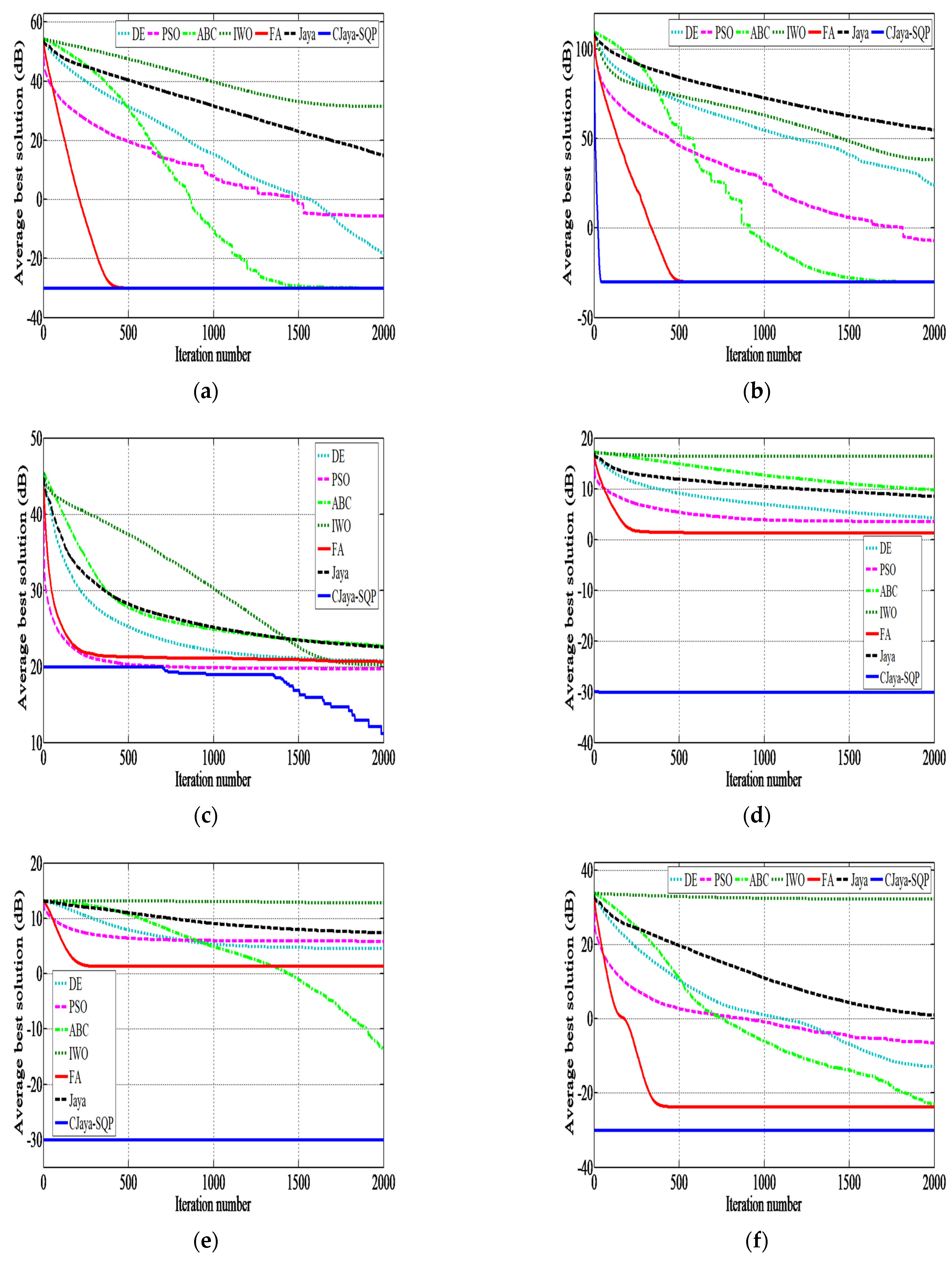
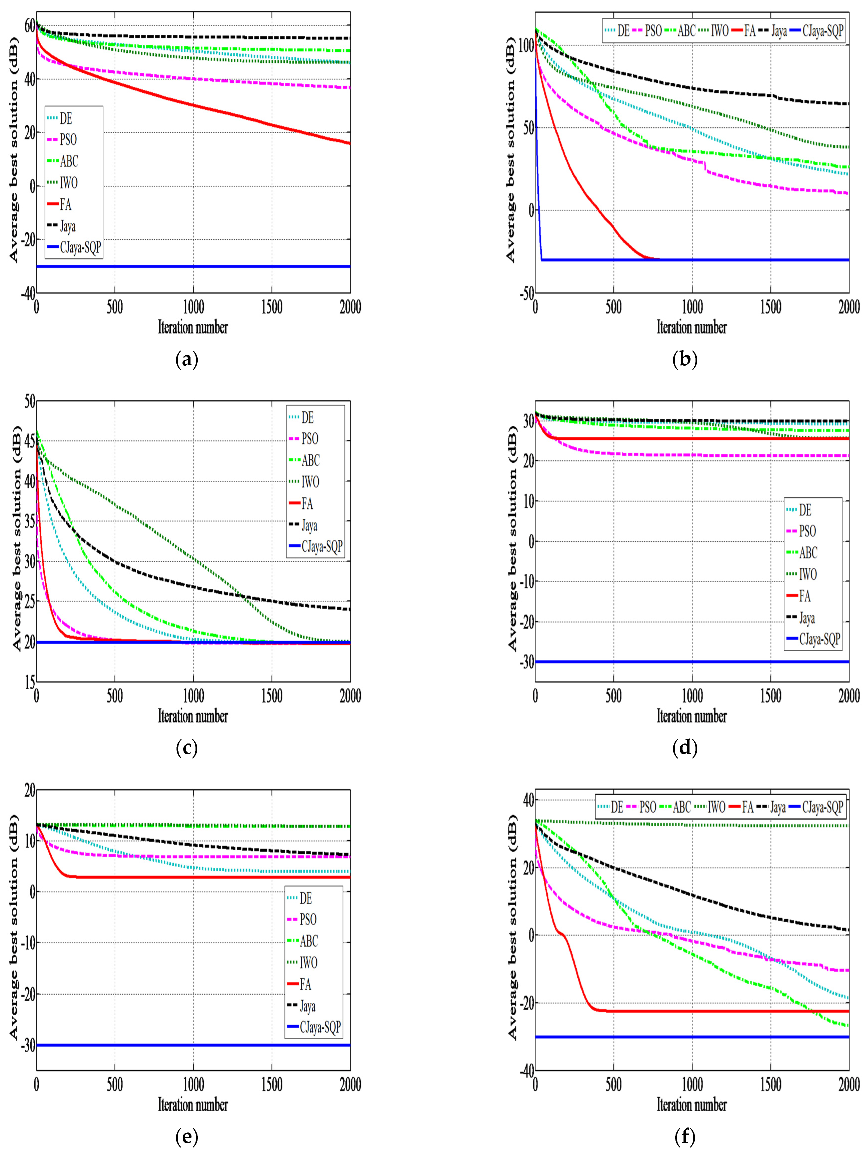
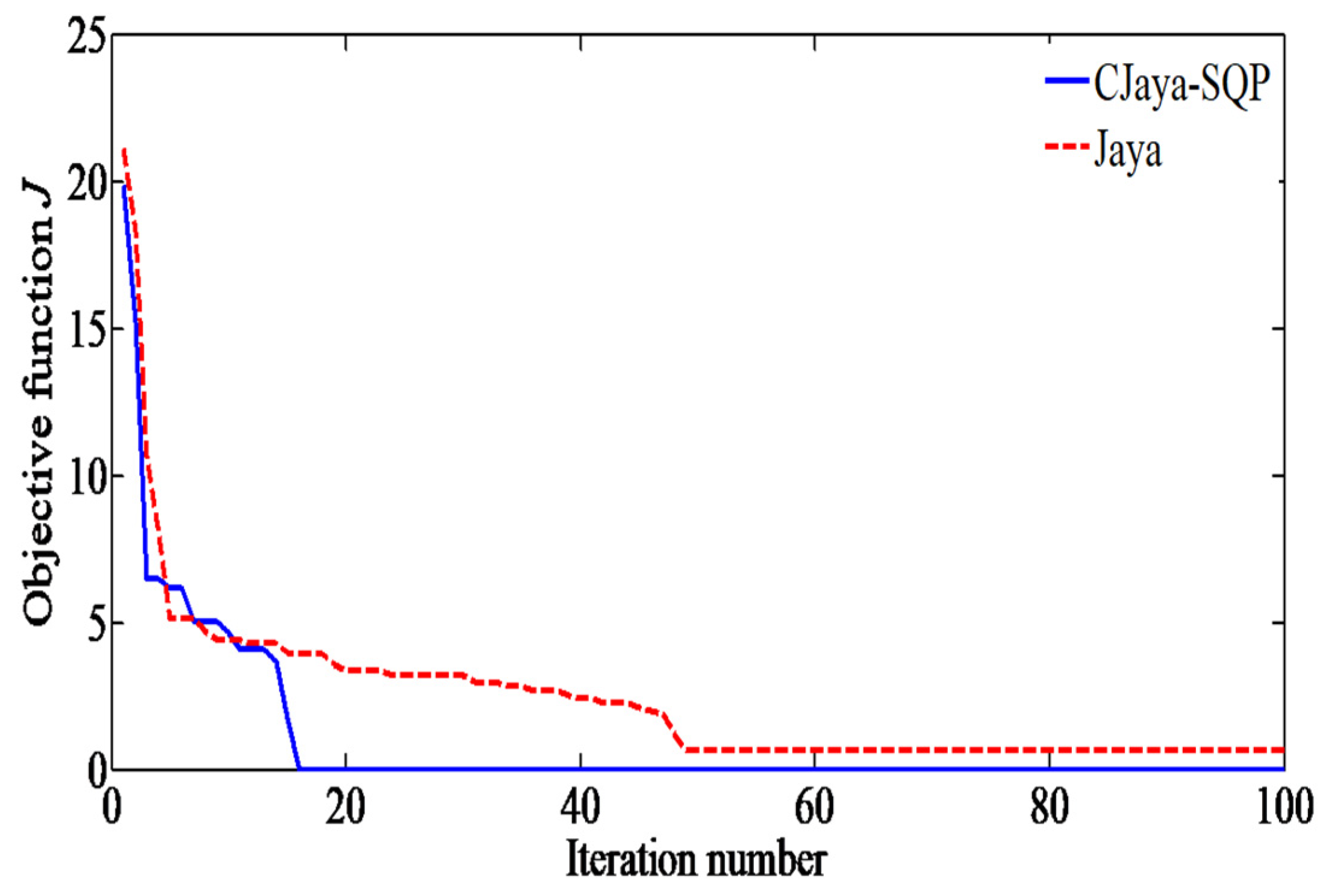
6.2.2. Comparison of Convergence and Success Ratios

In this experiment, the computational effort and consistency of the developed CJaya-SQP algorithm is compared with the conventional Jaya, DE, PSO, ABC, IWO and FA. For a fair comparison, each optimization algorithm is terminated when FEs is reached or when the best objective value is below the threshold value (T-Value) in each run. The comparative results of all the optimization algorithms regarding the mean function evaluations (MeanFEs) and success rate (SR) in the 30 runs are given in

Table 6. Mean function evaluations required to reach the threshold value and success rate by various algorithms for 30-dimensional functions over 30 runs.

Function		DE	PSO	ABC	IWO	FA	Jaya	CJaya-SQP
f1	MeanFEs	15,963	9556	11,655	65,471	8593.3	37,517	3.33
	SR (%)	100	100	100	100	100	100	100
f2	MeanFEs	NaN	NaN	NaN	NaN	19,125	NaN	8.06
	SR (%)	0	0	0	0	100	0	100
f3	MeanFEs	32,199	25,373	35,040	NaN	25,160	76,022.67	10.43
	SR (%)	100	100	100	0	100	100	100
f4	MeanFEs	25,470.67	16,504	20,672	NaN	14,408	56,173.33	1122.83
	SR (%)	100	100	100	0	100	100	100
f5	MeanFEs	NaN	NaN	57,856	NaN	NaN	603,80	17,826.21
	SR (%)	0	0	16.66	0	0	13.33	96.66
f6	MeanFEs	NaN	NaN	42,561.33	NaN	NaN	NaN	7.63
	SR (%)	0	0	100	0	0	0	100
f7	MeanFEs	NaN	NaN	NaN	NaN	NaN	NaN	20.46
	SR (%)	0	0	0	0	0	0	100
f8	MeanFEs	32,580.69	23,925	41,117.33	NaN	23,965.33	77,400	27.5
	SR (%)	96.66	53.33	100	0	100	86.66	100
f9	MeanFEs	24,464.76	16,008.89	31,547.69	NaN	16,073.68	61,088	23.5
	SR (%)	70	30	86.66	0	63.33	16.66	100
f10	MeanFEs	NaN	NaN	NaN	NaN	18,386.67	NaN	10.16
	SR (%)	0	0	0	0	100	0	100
f11	MeanFEs	39,573.33	44,388	NaN	NaN	25,192	NaN	11.90
	SR (%)	100	66.66	0	0	100	0	100
f12	MeanFEs	46,014.67	26,560	NaN	NaN	14,850.67	NaN	1278.66
	SR (%)	100	100	0	0	100	0	100
f13	MeanFEs	5794.66	1226.66	7540	45,032	834.66	15,921.33	36.76
	SR (%)	100	100	100	100	100	100	100
f14	MeanFEs	NaN	NaN	NaN	NaN	NaN	NaN	9.33
	SR (%)	0	0	0	0	0	0	100
f15	MeanFEs	NaN	NaN	NaN	NaN	NaN	NaN	23.56
	SR (%)	0	0	0	0	0	0	100
f16	MeanFEs	33,384.83	22,480	NaN	NaN	23,966.67	78,511.11	29.83
	SR (%)	96.66	3.33	0	0	100	30	100
f17	MeanFEs	26,200	17,637.33	47,376.67	NaN	16,048.57	64,885	25.43
	SR (%)	66.66	50	80	0	93.33	26.66	100

. NaN represents that algorithm fails to reach the T-Value during the 30 runs and boldface shows the best results.

Table 6 shows that CJaya-SQP algorithm requires the fewest values of MeanFEs to attain T-Value with 100% success rate for all the unimodal, multimodal and rotated problems, except for f₅ test function in which the success ratio is equal to 96.66%. It is also observed from the results that for f₇, f₁₄ and f₁₅ test functions, only CJaya-SQP succeeds to attain the T-Value in the 30 runs. Hence, the proposed algorithm is the most efficient among all the comparative algorithms.

6.2.3. Statistical Tests

To prove the significance of the suggested CJaya-SQP algorithm, the Friedman rank test is conducted for all unimodal, multimodal and rotated problems for the purpose of ranking all the considered algorithms.

Table 7. Friedman rank test for the ‘Mean’ and ‘SEM’ solutions obtained for 30-dimensional functions over 30 runs.

Test for Mean Solutions				Test for SEM Solutions
Algorithms	Friedman Value	Normalized Value	Rank	Algorithms	Friedman value	Normalized Value	Rank
DE	3.94	3.05	3	DE	4.05	3.85	3
PSO	4.05	3.13	4	PSO	4.23	4.02	4
ABC	4.52	3.50	5	ABC	4.82	4.59	5
IWO	5.82	4.51	6	IWO	5.52	5.25	6
FA	2.47	1.91	2	FA	2.70	2.57	2
Jaya	5.88	4.55	7	Jaya	5.58	5.31	7
CJaya-SQP	1.29	1.00	1	CJaya-SQP	1.05	1.00	1

presents the results of Friedman rank test based on the best mean solutions and the standard errors of means derived by all comparative algorithms. As can be observed from this table, CJaya-SQP has obtained the first rank followed by FA in both cases of mean and SEM solutions of all the benchmark functions.

6.3. Results for High-Dimensional Problems

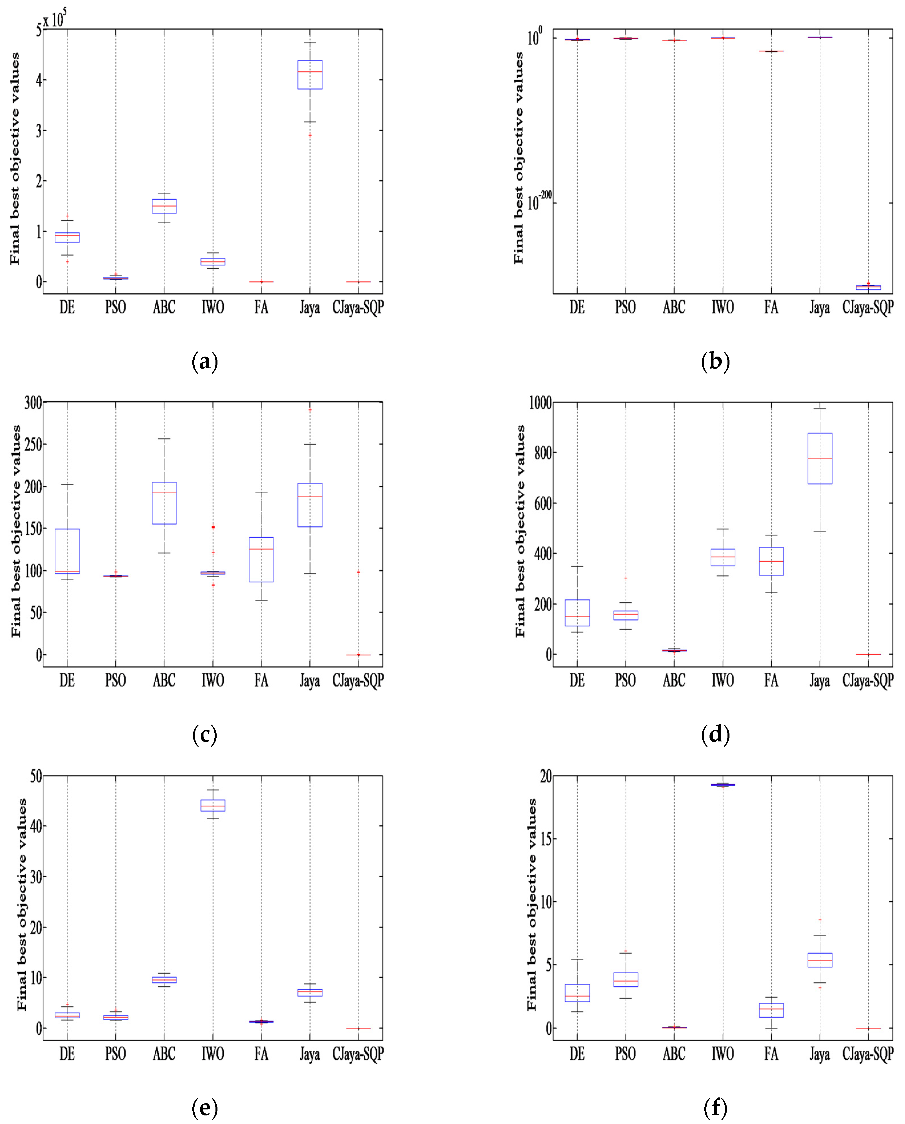
6.3.1. Comparison of Solution Accuracy

The results including the mean, the standard deviations and the standard error of means in 30 independent runs for the seven algorithms over 80,000 objective function evaluations on seventeen 100-dimensional functions are presented in

Table 8. Statistical results obtained by comparative algorithms for 100-dimensional functions over 30 runs with 80,000 function evaluations.

Function		DE	PSO	ABC	IWO	FA	Jaya	CJaya-SQP
f1	Mean	1.34 × 10−2	2.72 × 10−1	6.06 × 10−6	1.41 × 103	2.78 × 10−32	3.08 × 101	0.00
	SD	3.12 × 10−2	1.16 × 100	7.59 × 10−6	7.79 × 102	4.82 × 10−33	1.66 × 101	0.00
	SEM	5.69 × 10−3	2.12 × 10−1	1.38 × 10−6	1.42 × 102	8.80 × 10−34	3.03 × 100	0.00
f2	Mean	8.72 × 104	7.32 × 103	1.49 × 105	4.05 × 104	1.04 × 102	4.05 × 105	0.00
	SD	1.90 × 104	2.50 × 103	1.60 × 104	7.65 × 103	1.60 × 102	4.67 × 104	0.00
	SEM	3.48 × 103	4.57 × 102	2.92 × 103	1.39 × 103	2.92 × 101	8.53 × 103	0.00
f3	Mean	5.53 × 10−2	7.02 × 10−1	2.64 × 10−3	1.82 × 100	1.15 × 10−16	8.00 × 100	4.07 × 10−298
	SD	1.47 × 10−1	7.58 × 10−1	9.26 × 10−4	2.73 × 100	9.25 × 10−18	4.01 × 100	0.00
	SEM	2.69 × 10−2	1.38 × 10−1	1.69 × 10−4	5.00 × 10−1	1.69 × 10−18	7.33 × 10−1	0.00
f4	Mean	2.51 × 102	2.00 × 10−1	1.05 × 10−5	6.59 × 103	2.49 × 10−31	3.10 × 105	0.00
	SD	7.45 × 102	3.69 × 10−1	9.27 × 10−6	4.28 × 103	8.71 × 10−32	6.15 × 105	0.00
	SEM	1.36 × 102	6.74 × 10−2	1.69 × 10−6	7.82 × 102	1.59 × 10−32	1.12 × 105	0.00
f5	Mean	1.20 × 102	9.34 × 101	1.85 × 102	1.05 × 102	1.16 × 102	1.80 × 102	1.30 × 101
	SD	3.26 × 101	1.08 × 100	3.41 × 101	2.16 × 101	3.42 × 101	4.67 × 101	3.39 × 101
	SEM	5.95 × 100	1.98 × 10−1	6.24 × 100	3.96 × 100	6.26 × 100	8.54 × 100	6.19 × 100
f6	Mean	1.71 × 102	1.62 × 102	1.73 × 101	3.88 × 102	3.71 × 102	7.72 × 102	0.00
	SD	7.69 × 101	3.50 × 101	4.16 × 100	4.42 × 101	6.19 × 101	1.27 × 102	0.00
	SEM	1.40 × 101	6.39 × 100	7.59 × 10−1	8.07 × 100	1.13 × 101	2.32 × 101	0.00
f7	Mean	2.68 × 100	2.27 × 100	9.60 × 100	4.40 × 101	1.33 × 100	7.08 × 100	0.00
	SD	7.94 × 10−1	5.72 × 10−1	7.20 × 10−1	1.40 × 100	1.63 × 10−1	8.45 × 10−1	0.00
	SEM	1.45 × 10−1	1.04 × 10−1	1.31 × 10−1	2.56 × 10−1	2.97 × 10−2	1.54 × 10−1	0.00
f8	Mean	2.84 × 100	3.89 × 100	4.14 × 10−2	1.92 × 101	1.36 × 100	5.51 × 100	8.88 × 10−16
	SD	1.10 × 100	9.08 × 10−1	2.94 × 10−2	8.75 × 10−2	7.94 × 10−1	1.16 × 100	0.00
	SEM	2.01 × 10−1	1.65 × 10−1	5.38 × 10−3	1.59 × 10−2	1.45 × 10−1	2.13 × 10−1	0.00
f9	Mean	5.07 × 10−2	2.30 × 10−1	4.15 × 10−3	1.71 × 103	3.28 × 10−3	1.25 × 100	0.00
	SD	6.99 × 10−2	3.87 × 10−1	9.14 × 10−3	8.95 × 101	5.93 × 10−3	1.57 × 10−1	0.00
	SEM	1.27 × 10−2	7.07 × 10−2	1.67 × 10−3	1.63 × 101	1.08 × 10−3	2.86 × 10−2	0.00
f10	Mean	4.11 × 104	4.75 × 103	1.16 × 105	4.24 × 104	3.82 × 101	3.37 × 105	0.00
	SD	1.13 × 104	1.66 × 103	1.72 × 104	6.87 × 103	3.28 × 101	4.32 × 104	0.00
	SEM	2.07 × 103	3.04 × 102	3.14 × 103	1.25 × 103	5.99 × 100	7.89 × 103	0.00
f11	Mean	6.76 × 100	5.26 × 100	1.36 × 101	3.17 × 100	8.83 × 100	3.23 × 1012	1.54 × 10−296
	SD	3.64 × 100	3.51 × 100	5.57 × 100	4.48 × 100	7.97 × 100	1.77 × 1013	0.00
	SEM	6.65 × 10−1	6.41 × 10−1	1.01 × 100	8.19 × 10−1	1.45 × 100	3.23 × 1012	0.00
f12	Mean	1.56 × 102	1.12 × 101	4.11 × 102	6.75 × 103	1.38 × 10−18	2.81 × 106	0.00
	SD	2.53 × 102	2.40 × 101	3.49 × 102	6.01 × 103	2.52 × 10−18	6.79 × 106	0.00
	SEM	4.63 × 101	4.39 × 100	6.37 × 101	1.09 × 103	4.60 × 10−19	1.24 × 106	0.00
f13	Mean	9.81 × 101	9.44 × 101	9.65 × 101	1.01 × 102	9.45 × 101	2.53 × 102	9.89 × 101
	SD	9.85 × 100	2.00 × 100	1.50 × 100	1.57 × 101	1.80 × 101	1.82 × 102	2.12 × 10−2
	SEM	1.79 × 100	3.65 × 10−1	2.74 × 10−1	2.87 × 100	3.29 × 100	3.33 × 101	3.87 × 10−3
f14	Mean	8.33 × 102	1.38 × 102	5.72 × 102	3.68 × 102	3.60 × 102	9.88 × 102	0.00
	SD	1.29 × 102	2.69 × 101	3.98 × 101	5.52 × 101	6.10 × 101	4.36 × 101	0.00
	SEM	2.36 × 101	4.92 × 100	7.27 × 100	1.00 × 101	1.11 × 101	7.97 × 100	0.00
f15	Mean	2.38 × 100	2.40 × 100	9.63 × 100	4.43 × 101	1.25 × 100	7.29 × 100	0.00
	SD	7.40 × 10−1	4.94 × 10−1	7.86 × 10−1	1.71 × 100	1.52 × 10−1	8.45 × 10−1	0.00
	SEM	1.35 × 10−1	9.02 × 10−2	1.43 × 10−1	3.13 × 10−1	2.78 × 10−2	1.54 × 10−1	0.00
f16	Mean	2.51 × 100	4.87 × 100	1.89 × 101	1.93 × 101	1.95 × 100	5.41 × 100	8.88 × 10−16
	SD	6.20 × 10−1	8.23 × 10−1	2.68 × 100	7.75 × 10−2	3.91 × 10−1	9.34 × 10−1	0.00
	SEM	1.13 × 10−1	1.50 × 10−1	4.90 × 10−1	1.41 × 10−2	7.14 × 10−2	1.70 × 10−1	0.00
f17	Mean	1.28 × 10−2	9.16 × 10−2	1.10 × 10−3	1.72e × 103	4.76 × 10−3	1.42 × 100	0.00
	SD	1.27 × 10−2	1.36 × 10−1	1.75 × 10−3	8.97 × 101	6.39 × 10−3	5.93 × 10−1	0.00
	SEM	2.31 × 10−3	2.49 × 10−2	3.20 × 10−4	1.63 × 101	1.16 × 10−3	1.08 × 10−1	0.00

. It is obvious that the CJaya-SQP algorithm significantly outperforms the remaining algorithms for all unimodal, multimodal and rotated problems over the 30 runs, except for f₅ and f₁₃ functions. For f₅, the PSO algorithm obtains the best SD and SEM values, whereas CJaya-SQP provides the best mean result. For f₁₃, the PSO provides the best mean result and the proposed algorithm has the best SD and SEM results. Overall, the CJaya-SQP is the most competitive algorithm regarding solutions accuracy and ability to move away from local optimums for high dimensional problems.

In order to demonstrate the computational results, the box-plots are used to illustrate the distribution of results achieved by each algorithm over 30 independent runs on f₂, f₃, f₅, f₆, f₇ and f₈ conventional problems. These box-plots are illustrated in Figure 11. Compared to the conventional Jaya, the improvement by the proposed CJaya-SQP algorithm is obvious. Compared to other competitive algorithms, the CJaya-SQP also features an excellent performance in terms of robustness and solution quality, which is illustrated from the span of the solution distributions.

To further validate the computational results, the box-plots of best solutions produced by all optimization algorithms over 30 runs on f₁₀, f₁₁, f₁₂, f₁₄, f₁₅ and f₁₆ rotated problems are illustrated in Figure 12. It is obvious that the CJaya-SQP provides the highest solutions quality and it is the most robust among the other competitive algorithms.

6.3.2. Comparison of Convergence and Success Ratios

The effectiveness of the suggested algorithm to converge to an acceptable solution for the 100-dimensional problems over 30 runs is investigated by the computational effort expressed by MeanFEs and SR results given in

Table 9. Mean function evaluations required to reach the threshold value and success rate by various algorithms for 100-dimensional functions over 30 runs.

Function		DE	PSO	ABC	IWO	FA	Jaya	CJaya-SQP
f1	MeanFEs	74,322	66,373	43,039	NaN	12704	NaN	9.86
	SR (%)	66.66	60	100	0	100	0	100
f2	MeanFEs	NaN	NaN	NaN	NaN	NaN	NaN	12.5
	SR (%)	0	0	0	0	0	0	100
f3	MeanFEs	NaN	NaN	NaN	NaN	30140	NaN	14.3
	SR (%)	0	0	0	0	100	0	100
f4	MeanFEs	NaN	NaN	76,290.91	NaN	21,966.67	NaN	1498.66
	SR (%)	0	0	73.33	0	100	0	100
f5	MeanFEs	NaN	NaN	NaN	NaN	NaN	NaN	55,755.38
	SR (%)	0	0	0	0	0	0	86.66
f6	MeanFEs	NaN	NaN	NaN	NaN	NaN	NaN	12.03
	SR (%)	0	0	0	0	0	0	100
f7	MeanFEs	NaN	NaN	NaN	NaN	NaN	NaN	23.10
	SR (%)	0	0	0	0	0	0	100
f8	MeanFEs	NaN	NaN	NaN	NaN	26,793.33	NaN	31.16
	SR (%)	0	0	0	0	20	0	100
f9	MeanFEs	NaN	NaN	79,240	NaN	19,405.71	NaN	24.53
	SR (%)	0	0	3.33	0	70	0	100
f10	MeanFEs	NaN	NaN	NaN	NaN	NaN	NaN	16.43
	SR (%)	0	0	0	0	0	0	100
f11	MeanFEs	NaN	NaN	NaN	NaN	NaN	NaN	22.19
	SR (%)	0	0	0	0	0	0	100
f12	MeanFEs	NaN	NaN	NaN	NaN	32,870.67	NaN	1564
	SR (%)	0	0	0	0	100	0	100
f13	MeanFEs	NaN	NaN	NaN	NaN	NaN	NaN	NaN
	SR (%)	0	0	0	0	0	0	0
f14	MeanFEs	NaN	NaN	NaN	NaN	NaN	NaN	20.76
	SR (%)	0	0	0	0	0	0	100
f15	MeanFEs	NaN	NaN	NaN	NaN	NaN	NaN	26.86
	SR (%)	0	0	0	0	0	0	100
f16	MeanFEs	NaN	NaN	NaN	NaN	NaN	NaN	33.73
	SR (%)	0	0	0	0	0	0	100
f17	MeanFEs	NaN	NaN	NaN	NaN	19,456.47	NaN	29.36
	SR (%)	0	0	0	0	56.66	0	100

. It can be observed that CJaya-SQP produces the fewest MeanFEs to attain an acceptable solution and the highest success rate among all other algorithms. With the exception of f₅ benchmark function in which the SR is equal to 86.66%, the proposed algorithm achieves 100% success ratio for all unimodal, multimodal and rotated problems. For f₁₃, all algorithms failed to converge to an acceptable solution. It is also observed from the results that except for the proposed CJaya-SQP, the remaining comparative algorithms failed to converge to the threshold value for f₂, f₅, f₆, f₇, f₁₀, f₁₁, f₁₄, f₁₅ and f₁₆ test functions in the 30 runs. Hence, the performance of CJaya-SQP is significantly superior to other optimization algorithms. It is worth mentioning that the conventional Jaya algorithm failed to produce a feasible solution for all 100-dimensional problems, which points out its weak global search behavior. Owing to the modifications embedded into Jaya, the CJaya-SQP presents high speed convergence and efficiency.

To further evaluate the exploitation ability of the proposed CJaya-SQP compared to the rest of algorithms, the convergence characteristics of f₁, f₄, f₅, f₇, f₈ and f₉ conventional problems are shown in Figure 13. It is worth noting that the objective function values are shifted by a gap of 10⁻³ because of some zero values, and therefore they can be plotted ona semi-log scale. It is observed from Figure 13 that CJaya-SQP algorithm is the best performing in terms of solutions quality and convergence speed.

The convergence characteristics of CJaya-SQP compared to other algorithms on f₁₀, f₁₂, f₁₃, f₁₄, f₁₆ and f₁₇ rotated problems are illustrated in Figure 14. It is obvious that the proposed algorithm has a faster convergence speed in all rotated problems than the remaining algorithms. It can be concluded that CJaya-SQP is a powerful algorithm for the design of complex optimization problems.

6.3.3. Statistical Tests

To statistically evaluate the performance of all comparative algorithms applied in the experiments, the Friedman rank test is conducted on the best mean solutions and the standard errors of means obtained for the 100-dimensional problems. It is obvious from the results given in

Table 10. Friedman rank test for the ‘Mean’ and ‘SEM’ solutions obtained for 100-dimensional functions over 30 runs.

Test for Mean Solutions				Test for SEM Solutions
Algorithms	Friedman Value	Normalized Value	Rank	Algorithms	Friedman Value	Normalized Value	Rank
DE	4.17	3.39	4	DE	4.58	3.91	5
PSO	3.52	2.86	3	PSO	3.58	3.05	3
ABC	4.35	3.53	5	ABC	3.82	3.26	4
IWO	5.70	4.63	6	IWO	5.05	4.31	6
FA	2.64	2.14	2	FA	3.35	2.86	2
Jaya	6.35	5.16	7	Jaya	6.41	5.47	7
CJaya-SQP	1.23	1.00	1	CJaya-SQP	1.17	1.00	1

that CJaya-SQP is ranked first in the case of mean and SEM solutions of all benchmark functions. It is worth noting that in 30- and 100-dimensional problems, the original Jaya algorithm stands last among all optimization algorithms in the case of mean and SEM solutions, which reflects its weak searching capability. Thanks to the chaotic system and the SQP method introduced in Jaya, the developed algorithm presents a high searching ability, efficiency and robustness for solving high dimensional problems.

7. Practical Application

In this section, the applicability of the proposed RPL sensitivity-based approach for determining the best location of the SVC device is tested on the four-machine, two-area power system. Moreover, the robustness and feasibility of the proposed hybrid CJaya-SQP algorithm for optimal design of PSSs and SVC controllers are demonstrated using a multi-objective optimization problem. The single line diagram of the test system is shown in Figure 15. Each area includes two generating units with a rating of 900 MVA and 20 kV for each unit. There is a power transfer of 413 MW from area 1 to area 2. This test system is used for studies on power system stability. All system data can be found in detail in [56].

7.1. PSSs Locations

To determine the optimum locations of PSSs, the participation factors method [56] is applied. The system electromechanical modes and their associated frequencies, damping ratios and machine participation factors (PF) without installing PSSs are given in

Table 11. Test system electromechanical modes and participation factor analysis.

Eigenvalues	Frequency	Modes	Damping Ratio	Generators	State Variables	$\mathit{P}\mathit{F}$
0.0720 ± j3.7192	0.5919	Interarea	−0.0194	$\mathrm{G}1$	$\delta , \omega$	1.0000, 1.0000
				$\mathrm{G}2$	$\delta , \omega$	0.6012, 0.6012
				$\mathrm{G}3$	$\delta , \omega$	0.7181, 0.7181
				$\mathrm{G}4$	$\delta , \omega$	0.7445, 0.7445
−0.2166 ± j5.9569	0.9481	Local	0.0363	$\mathrm{G}1$	$\delta , \omega$	0.8053, 0.8053
				$\mathrm{G}2$	$\delta , \omega$	1.0000, 1.0000
				$\mathrm{G}3$	$\delta , \omega$	0.0316, 0.0316
				$\mathrm{G}4$	$\delta , \omega$	0.0119, 0.0119
−0.2161 ± j6.1273	0.9752	Local	0.0352	$\mathrm{G}1$	$\delta , \omega$	0.0145, 0.0145
				$\mathrm{G}2$	$\delta , \omega$	0.0229, 0.0229
				$\mathrm{G}3$	$\delta , \omega$	0.9941, 0.9941
				$\mathrm{G}4$	$\delta , \omega$	1.0000, 1.0000

. It can be observed from Table 11 that the power system exhibits three electromechanical modes. For the poorly damped local mode of area 1, the generator G2 is the most effective location for installing PSS as it has the highest participation factor for this mode. Similarly, the generator G4 is the suitable candidate location of PSS for the local mode of area 2. In order to increase the damping performances of the unstable inter-area mode, the generator G1 is the best location of PSS. Therefore, the generators G1, G2 and G4 are the optimum locations for installing the PSSs.

7.2. SVC Location and Input Signal

In order to select the optimal location of the SVC controller, the proposed RPL sensitivity approach is applied to the test power system.

Table 12. Values of real power loss sensitivity index.

Bus No.	Base Case	% Load Increase
		10	15	20	25	30
Bus 7	0.0038	0.0055	0.0064	0.0073	0.0081	0.0087
Bus 8	0.0279	0.0390	0.0448	0.0509	0.0574	0.0646

presents the sensitivities of the total system RPL with respect to the injected reactive power at load buses 7 and 8. It can be observed from Table 12 that bus 8 is the most sensitive bus due to thehighest absolute value of sensitivity indices. Moreover, this bus is connected to the heaviest load in the system. Hence, bus 8 is the most effective location for installing an SVC controller. This indicates that the placement of SVC device at bus 8 will minimize the total RPL of the power system more than the placement in other buses.

In order to boost the damping performances, especially for the inter-area power oscillations, the rotor speed deviations of the generators G1 and G3 $({\omega }_{G1}-{\omega }_{G3})$ which is observable for the inter-area mode is chosen as the input signal of the SVC based damping controller. The generator G1 is selected since it presents the highest participation factor for the unstable inter-area mode of the test system as it is shown in Table 11. Finally, the chosen SVC input signal agrees with that considered in [57].

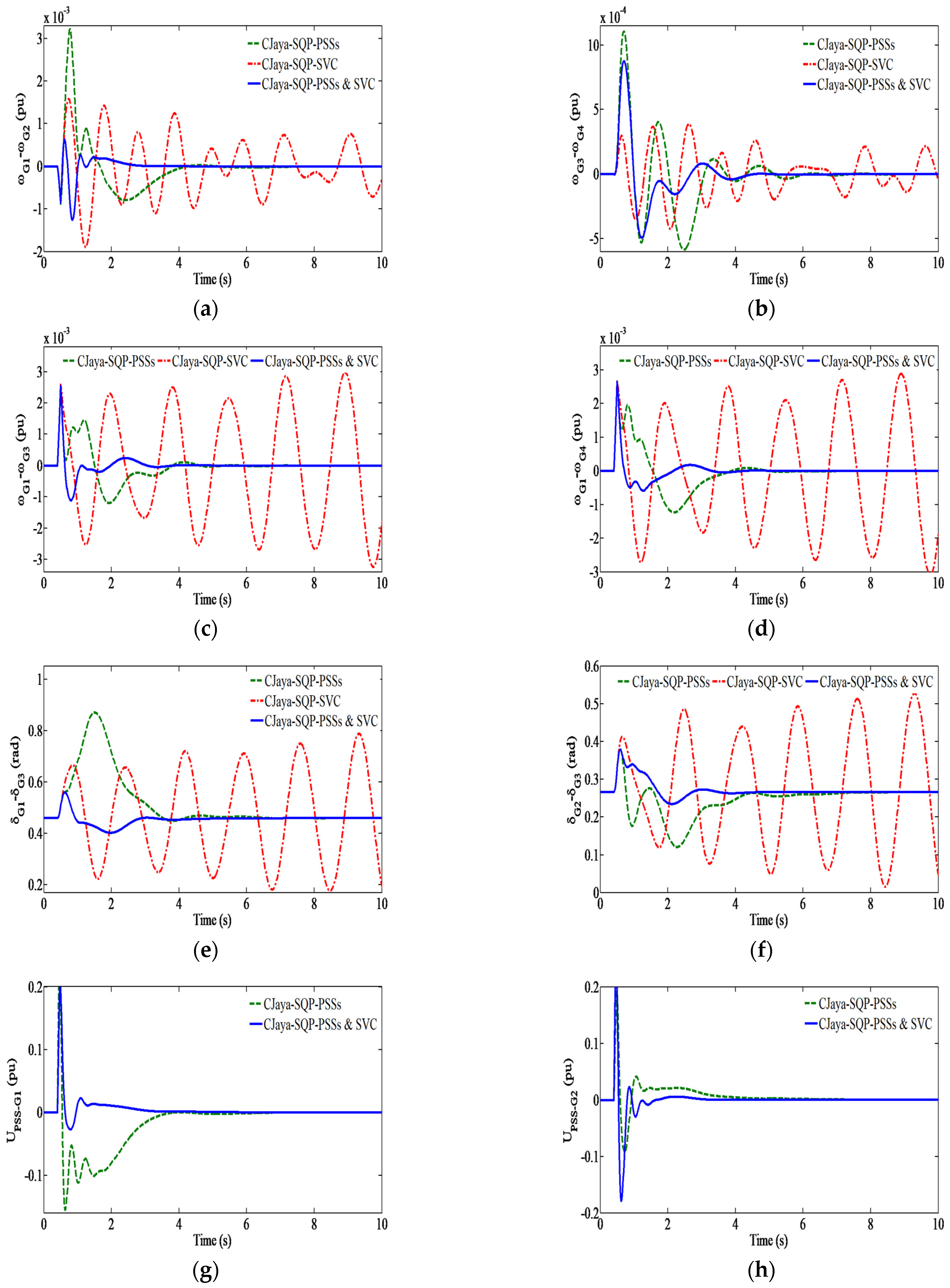
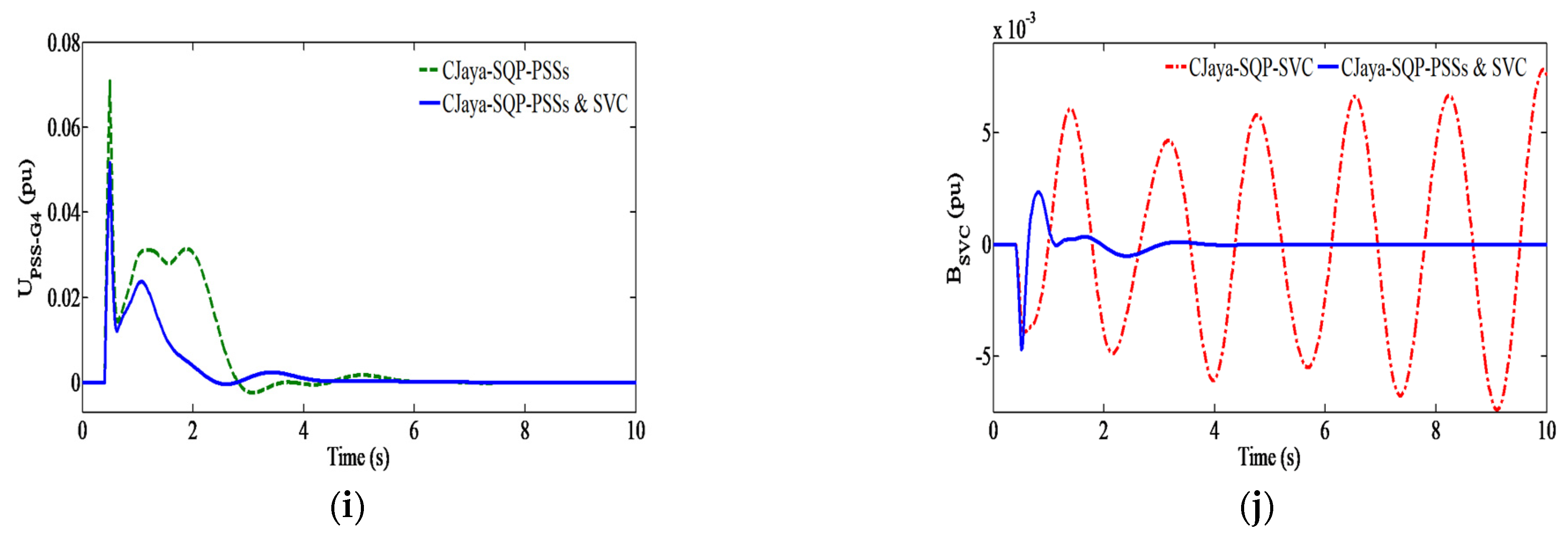
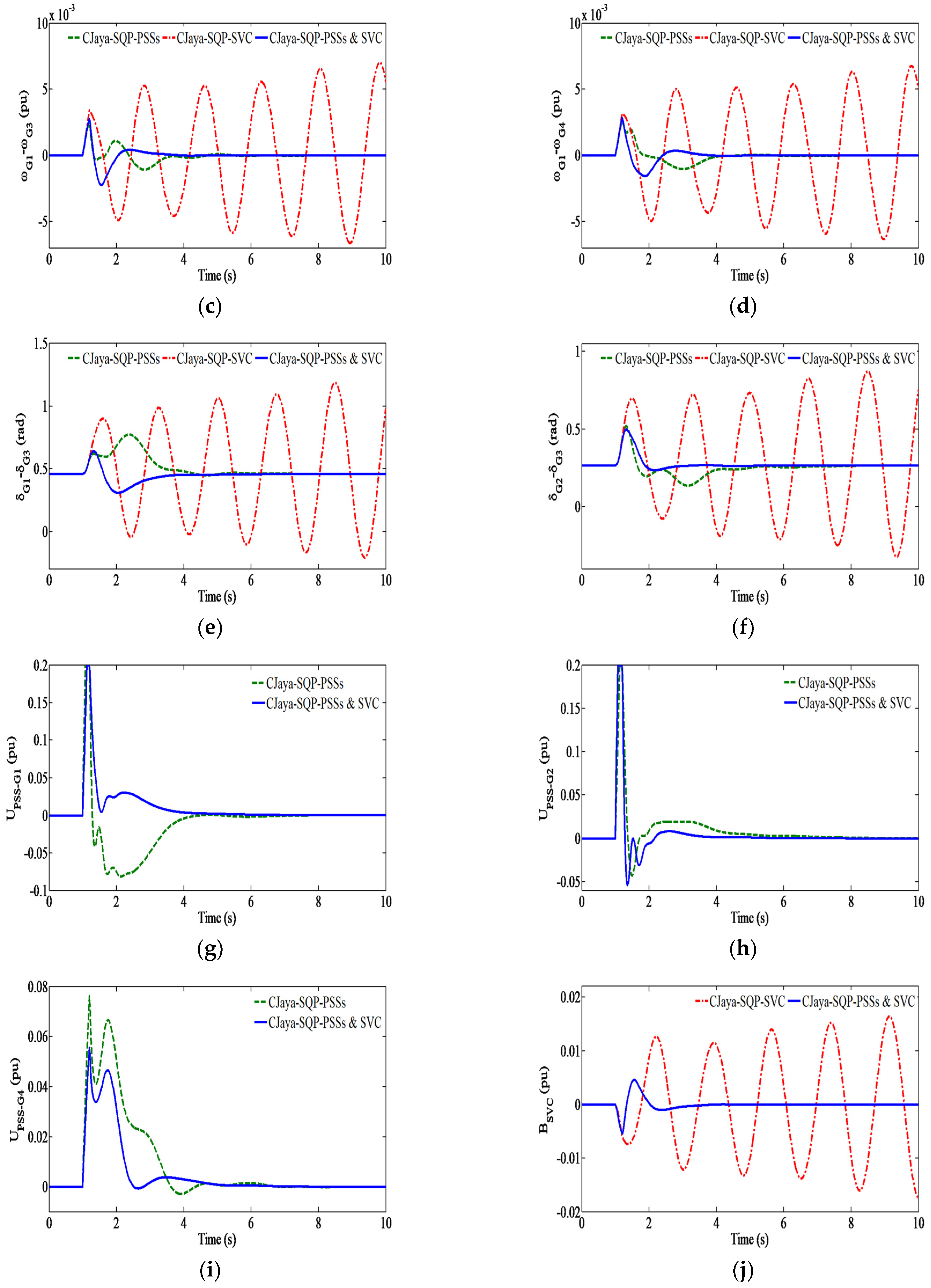
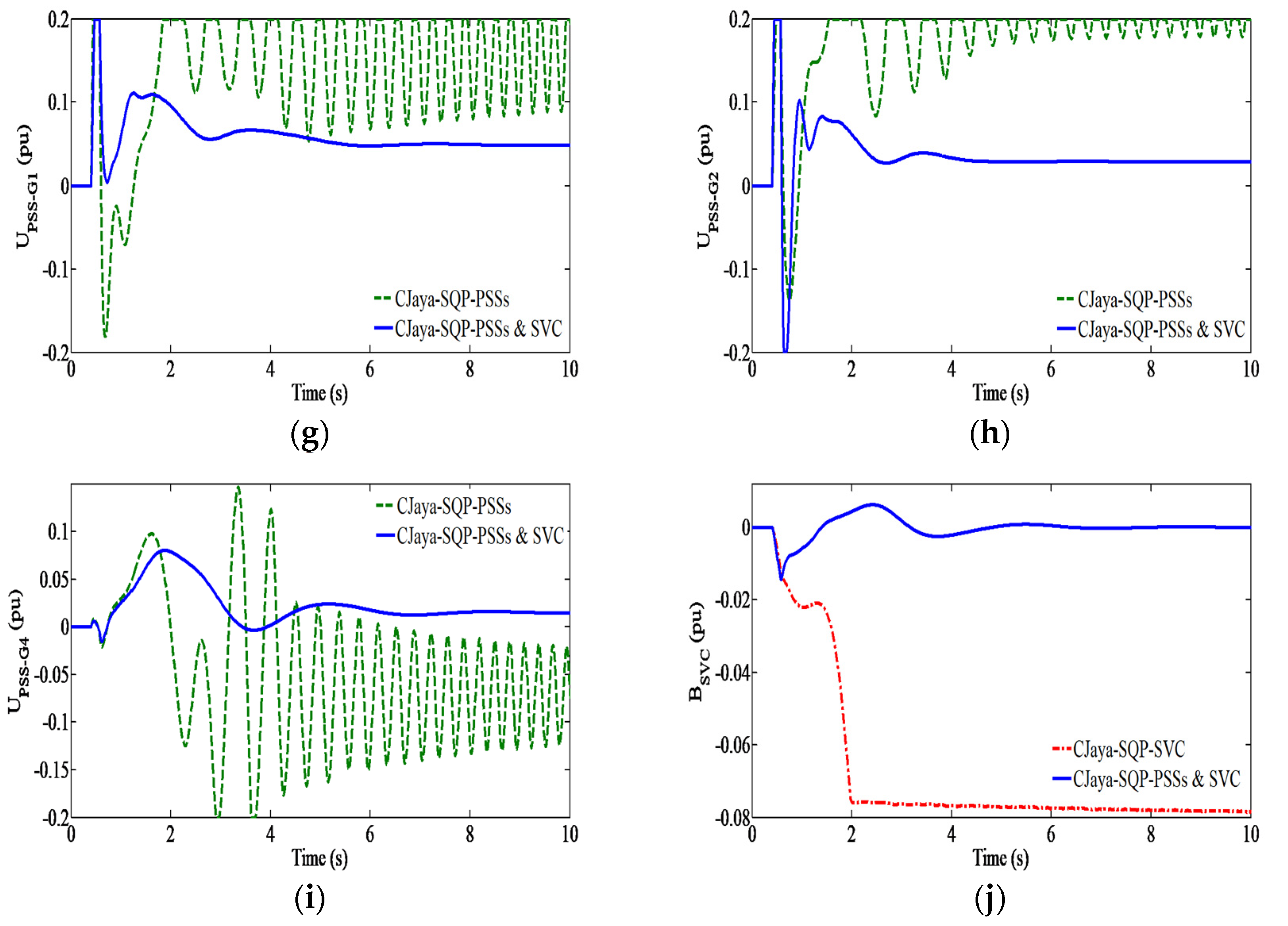
7.3. Damping Controllers Design and Robustness Analysis

In this section, the coordination design problem of PSSs and SVC-based control to boost the power network stability is handled as an optimization problem. The proposed CJaya-SQP algorithm is applied to the study system to determine the optimal parameters for the three installed PSSs and the SVC controller. In this study, the CJaya-SQP parameters, including the iteration number $MaxIter$ and the population size $NP$ are set to 100 and the maximum iteration number of the CLS $k_{\max }$ is set to 20. To highlight the effectiveness of the suggested coordinated PSSs and SVC controllers, the CJaya-SQP-based PSSs (Jaya-SQP-PSSs) and the Jaya-SQP-based SVC controller (Jaya-SQP-SVC) are presented and their performances are compared to the proposed Jaya-SQP-based coordinated controller (Jaya-SQP-PSSs&SVC). The D-shape sector boundaries ${\sigma }_0$ and ${\xi }_0$ are set as: −2 and 0.3, respectively. These values are determined from various analyses of the system eigenvalues.

The convergence characteristics of the proposed CJaya-SQP compared to the original Jaya for the proposed controllers are shown in Figure 16. It is clear that the CJaya-SQP method presents better characteristics in terms of convergence speed and solutions quality compared to the Jaya algorithm. The optimal PSSs and SVC parameters are shown in

Table 13. Optimal value of PSSs and SVC parameters obtained by C Jaya-SQP method.

	Uncoordinated Design				Coordinated Design
	PSS-G1	PSS-G2	PSS-G4	SVC	PSS-G1	PSS-G2	PSS-G4	SVC
K	17.5059	28.0717	11.5571	33.3058	32.2919	30.2838	9.2705	11.6793
T1	1.1324	1.1831	1.2220	0.1464	0.9337	0.7207	1.8364	1.3573
T2	0.2664	0.6197	0.5310	0.8140	0.6893	0.5714	1.3917	0.9393
T3	1.4371	1.1725	1.4376	1.6985	0.8732	1.5084	1.3293	1.0909
T4	1.0159	1.3452	1.1442	1.2474	0.6431	0.6918	0.5001	1.3336

. As it can be seen from Figure 16, the final value of the objective function J with the CJaya-SQP method is $J=0$. This means that all the electromechanical modes are successfully placed in the desired area characterized by $\sigma <{\sigma }_0$ and $\xi >{\xi }_0$.

Table 14. Test system electromechanical modes and related damping ratios for different cases.

Case	Eigenvalues	Damping Ratios
CJaya-SQP-PSSs	−2.7659 ± j7.7039	0.3379
	−2.1961 ± j1.8797	0.7597
	−1.2187 ± j2.0866	0.5043
CJaya-SQP-SVC	0.0731 ± j3.7180	−0.0197
	−0.2164 ± j5.9569	0.0363
	−0.2167 ± j6.1283	0.0353
CJaya-SQP-PSSs&SVC	−2.7881 ± j7.6715	0.3416
	−2.6014 ± j1.9392	0.8018
	−2.0017 ± j3.2075	0.5294

depicts the electromechanical modes and related damping ratios to three system design methodologies.

It can be inferred from Table 14 that the system with the CJaya-SQP-SVC controller is unstable. In addition, only the CJaya-SQP-based coordinated controller succeeds in shifting all the electromechanical modes to the D-shape region and the damping factors are significantly improved. Moreover, the damping ratios are clearly enhanced by the coordinated controller. Hence, the power network damping performances are evidently boosted with the proposed coordinated approach in comparison with SVC and PSSs tuned individually.

To verify the effectiveness and robustness of the proposed CJaya-SQP-based tuned controllers in the damping of EMOs, nonlinear simulations are carried out for different scenarios. The behavior of the test system is evaluated for 10s. It should be emphasized that the robustness of the proposed controllers must be evaluated for the network topology, system loading condition and different fault disturbances in the studied system. To reach this goal, we propose four scenarios that simulate severe contingencies by changing the fault types and system loading conditions. These scenarios are summarized as follows:

Scenario I: Nominal loading, a three phase fault of six cycle duration occurs at bus 7 at $t=0.4 \mathrm{s}$ and it is removed by tripping the faulted line with successful reclosure after 100 ms.

Scenario II: Nominal loading, a load curtailment contingency of twelve cycle duration is applied at bus 7 at $t=1 \mathrm{s}$.

Scenario III: Nominal loading, a ten cycle three phase fault occurs at bus 7 at $t=0.4 \mathrm{s}$ and it is removed by an appropriate circuit breaker (outage of one of the tie lines connecting buses 7 and 8).

Scenario IV: Heavy loading (143% of nominal loading), a load curtailment contingency of twelve cycle duration occurs at bus 7 at $t=1 \mathrm{s}$.

Scenario I: A three phase fault of six cycle duration at bus 7 at $t=0.4 \mathrm{s}$ is applied in one of the tie lines. The fault is cleared by opening the faulted line with successful reclosure after 100 ms. The behavior of the test system is evaluated for 10 s. The local and inter-area mode responses with the coordinated and uncoordinated tuning of PSSs and SVC via CJaya-SQP are shown in Figure 17a–d. These figures show the speed deviations of G1–G2, G3–G4, G1–G3 and G1–G4. The rotor angle responses of generators G1 and G2 with respect to the swing generator G3 are provided by Figure 17e,f. It is clear from the results that both the CJaya-SQP-PSSs and CJaya-SQP-PSSs&SVC controllers are able to mitigate the EMOs and stabilize the power system. Moreover, the proposed coordinated CJaya-SQP-PSSs&SVC provides better damping characteristics than the CJaya-SQP-PSSs controller. Hence, the coordinated design method has an excellent capability to improve the dynamic stability performance and damping the low frequency oscillations quickly and efficiently.

The responses of the PSSs stabilizing signals and SVC susceptance represented respectively by U_PSS-G1, U_PSS-G2, U_PSS-G4 and B_SVC are shown in Figure 17g–j. It can be concluded that the coordinated tuning of PSSs and SVC controllers has a strong ability to reduce the control effort more than CJaya-SQP-PSSs and CJaya-SQP-SVC, helping the power system to damp out the EMOs with a high speed. This confirms the potential of the suggested CJaya-SQP-based coordinated controller to boost the system damping performances.

Scenario II: In this scenario, the performance of the CJaya-SQP-based tuned controllers is also tested under load curtailment. At t = 1 s, the load at bus 7 is disconnected for 200 ms. Figure 18 illustrates the system dynamic response for the considered load curtailment contingency. Figure 18a,b show the speed deviation response of G1-G2 and G3-G4 and depict the local mode responses of area 1 and area 2 using the three system design methodologies. Figure 18c,d show the speed deviation response of G1-G3 and G1-G4 that illustrate the inter-area mode response using the coordinated and uncoordinated tuning of SVC and PSSs via the CJaya-SQP method. The rotor angle responses of generators G1 and G2 with respect to G3 are shown in Figure 18e,f. It can be observed from these figures that the CJaya-SQP-SVC controller is unable to mitigate both local and inter-area mode of oscillations. Moreover, it is evident that both the CJaya-SQP-based PSSs and the CJaya-SQP-based coordinated controller have the ability to damp out the local and inter-area oscillations and stabilize the test system. Moreover, it can be seen that the proposed CJaya-SQP-PSSs&SVC controller for damping the EMOs is robust and provides the best damping performances to the local and inter-area oscillations.

Figure 18g–j show the SVC susceptance response and the PSSs output signals responses at generators G1, G2 and G4. It can be found from these figures that using the CJaya-SQP-based coordinated controller, the power system is controlled better than the CJaya-SQP-PSSs and thus dampens the local and inter-area oscillations quickly and efficiently.

Scenario III: To highlight the robustness of the coordinated design approach, a three phase fault and transmission line outage are simultaneously considered. In this scenario, a ten cycle three phase fault occurs at bus 7 at $t=0.4 \mathrm{s}$ in one of the tie lines. The fault is removed by an appropriate circuit breaker. Therefore, the power system operates with one of the tie lines between two areas. The speed deviations and the rotor angle responses under the considered fault are shown in Figure 19a–f. Assessment of these figures reveals that both the CJaya-SQP-PSSs and CJaya-SQP-SVC controllers have an inferior effect on the local oscillations and they are insufficient to dampen the inter-area oscillations. It is also observed from Figure 19a–d that the proposed CJaya-SQP-based coordinated controller has the potential to grant superior damping performances of the inter-area and local oscillations, when compared to the uncoordinated tuning of PSSs and SVC controllers. Furthermore, by the use of the coordinated CJaya-SQP-PSSs&SVC controller, the EMOs are quickly damped and the system overshoot and undershoot are greatly improved.

The responses of the PSSs stabilizing signals and the SVC susceptance under the considered fault are shown in Figure 19g–j. These figures show that using the proposed CJaya-SQP-based coordinated controller reduces greatly the control effort of the test system, and therefore the power system oscillations are quickly damped by modulating the stabilizing signals and the susceptance of PSSs and SVC simultaneously.

Scenario IV: To further validate the robustness of the CJaya-SQP-based coordinated controller in mitigating the power system oscillations, another severe contingency is applied by changing the loading condition of the studied system from nominal to heavy loading (143% of nominal loading). In this scenario, a load curtailment contingency of twelve cycle duration occurs at bus 7 at $t=1 \mathrm{s}$. Figure 20 shows the system dynamic response under this type of contingency. The inter-area and local oscillation modes with the CJaya-SQP-based tuned controllers are shown in Figure 20a–d. The rotor angle responses of generators G1 and G2 with respect to G3 are given by Figure 20e,f. From these figures, it is clear that the CJaya-SQP-PSSs and CJaya-SQP-SVC controllers fail to damp out both local and inter-area oscillations and thus the power system is unstable under this contingency. Moreover, only the proposed coordinated CJaya-SQP-PSSs&SVC controller succeeds to stabilize the power system and mitigates both the local and inter-area oscillations quickly and efficiently under this load curtailment contingency and change in system operating condition.

The PSSs output signals at generators G1, G2 and G4 and the SVC susceptance responses are shown in Figure 20g–j. It can be seen from these figures that the proposed coordinated controller achieves the best control performance, thus increasing the stability performance despite the considerable change in the operating condition of the test system. All the reported results have proved that the coordination design of PSSs and SVC controllers by the proposed CJaya-SQP algorithm significantly outperforms the individual design of PSSs and SVC in increasing the damping performances and enhancing the system’s dynamic stability under all considered contingencies presented in scenarios I–IV.

7.4. Quantify the Enhancement of Proposed Approach

In this section, to demonstrate the performance of the CJaya-SQP-PSSs&SVC controller in comparison to the uncoordinated tuning of PSSs and SVC controllers regarding time-domain characteristics of local and inter-area oscillations, the integral of time absolute error (ITAE) criterion is introduced as follows:

$$ITA{E}_1={\displaystyle {\int }_0^{t_{sim}}t\left(\left|{\omega }_1-{\omega }_3\right|+\left|{\omega }_1-{\omega }_4\right|+\left|{\omega }_2-{\omega }_3\right|+\left|{\omega }_2-{\omega }_4\right|\right)} dt$$

(28)

$$ITA{E}_2={\displaystyle {\int }_0^{t_{sim}}t\left(\left|{\omega }_1-{\omega }_2\right|+\left|{\omega }_3-{\omega }_4\right|\right)} dt$$

(29)

where $t_{sim}$ denotes the simulation time which is chosen to be 10 s. ITAE₁ and ITAE₂ are two performance indices used to provide a clear perspective of the inter-area and local mode responses, respectively. The numerical results of these indices for all four suggested scenarios are given in

Table 15. Numerical results of ITAE₁ performance index for four suggested scenarios.

Controller type	ITAE1 (tsim = 10 s)
	Scenario I	Scenario II	Scenario III	Scenario IV	Total
CJaya-SQP-PSSs	0.0141	0.0192	9.0501	3.9026	12.9860
CJaya-SQP-SVC	0.3100	0.6942	29.7768	19.3631	50.1441
CJaya-SQP-PSSs&SVC	0.0049	0.0122	0.0778	0.0988	0.1937

and

Table 16. Numerical results of ITAE₂ performance index for four suggested scenarios.

Controller type	ITAE2 (tsim = 10 s)
	Scenario I	Scenario II	Scenario III	Scenario IV	Total
CJaya-SQP-PSSs	0.0064	0.0095	0.0698	0.4432	0.5289
CJaya-SQP-SVC	0.0286	0.0468	0.0941	0.9933	1.1628
CJaya-SQP-PSSs&SVC	0.0016	0.0040	0.0075	0.0097	0.0228

. It is worth noting that the lower values of the ITAE performance index point out the better system dynamic responses regarding damping performances and time-domain characteristics.

From the results given in Table 15, it is clear that the total values of ITAE₁ for CJaya-SQP-PSSs and CJaya-SQP-SVC controllers are respectively decreased by 98.51% and 99.61% to 0.1937 for the CJaya-SQP-PSSs&SVC controller. This confirms that the coordinated tuning of PSSs and SVC controllers via the CJaya-SQP method has the best system responses in terms of damping performances and time-domain characteristics of the inter-area oscillations. Additionally, it is evident from Table 16 that the total values of ITAE₂ for the individual design of PSSs and SVC controllers are respectively decreased by 95.69% and 98.04% to 0.0228 for the CJaya-SQP-PSSs&SVC controller. This proves that the CJaya-SQP-based coordinated controller provides superior damping performances to the local oscillations when compared to the uncoordinated tuning of PSSs and SVC controllers.

According to the abovementioned results, it can be concluded that the system damping performances for all of the proposed scenarios are evidently boosted by the coordinated design of PSSs and SVC conducted under the proposed CJaya-SQP method.

8. Conclusions and Perspectives

This paper investigates the application of PSSs and SVC controllers in increasing the damping of EMOs. As a first step in the design approach of controllers, a new hybrid algorithm called CJaya-SQP, by integrating CJaya with the SQP method, is developed. This hybrid algorithm incorporates CJaya as a global search procedure to extract a near optimum solution and increase the convergence speed and SQP as a local level search for further adjustment of this solution. In the second step, a new RPL sensitivity-based approach is suggested for selecting the most appropriate location for the SVC device. The performance of the suggested CJaya-SQP method is highlighted using a set of benchmark optimization problems. Compared with the conventional Jaya and other recognized algorithms, the proposed hybrid CJaya-SQP method presents better characteristics in terms of solution accuracy, convergence speed, success ratios and robustness. Finally, the proposed method is applied on an electric power system to handle the coordination tuning problem of PSSs and SVC controllers by minimizing an eigenvalue-based objective function. The performance of the coordinated strategy conducted under our proposed method is demonstrated through eigenvalue analysis, nonlinear simulations and performance index results under different contingencies and loading conditions. The obtained results prove the robustness of the proposed CJaya-SQP-based coordinated controller for changes in the system operating condition and faults type and its superiority over SVC and PSSs controllers tuned individually.

This research study is not only significant in terms of its applicability in the power systems field, but also contributes significantly to the research and development of optimization algorithms since the proposed CJaya-SQP can be used by other researchers to evaluate the efficiency and robustness of their algorithms. It can also be utilized in several engineering design applications. For future work, the authors will extend the proposed method for hybrid power networks by considering various types of FACTS devices.

References

1. Su, Q.; Khan, H.U.; Khan, I.; Choi, B.J.; Wu, F.; Aly, A.A. An optimized algorithm for optimal power flow based on deep learning. Energy Rep. 2021, 7, 2113–2124. [Google Scholar] [CrossRef]
2. Farah, A.; Guesmi, T.; Hadj Abdallah, H.; Ouali, A. A novel chaotic teaching–learning-based optimization algorithm for multi-machine power system stabilizers design problem. Int. J. Electr. Power Energy Syst. 2016, 77, 197–209. [Google Scholar] [CrossRef]
3. Welhazi, Y.; Guesmi, T.; Hadj Abdallah, H. Eigenvalue Assignments in Multimachine Power Systems using Multi-Objective PSO Algorithm. Int. J. Energy Optim. Eng. 2015, 4, 33–48. [Google Scholar] [CrossRef] [Green Version]
4. Hu, W.; Liang, J.; Jin, Y.; Wu, F. Model of Power System Stabilizer Adapting to Multi-Operating Conditions of Local Power Grid and Parameter Tuning. Sustainability 2018, 10, 2089. [Google Scholar] [CrossRef] [Green Version]
5. Jolfaei, M.G.; Sharaf, A.M.; Shariatmadar, S.M.; Poudeh, M.B. A hybrid PSS-SSSC GA-stabilization scheme for damping power system small signal oscillations. Int. J. Electr. Power Energy Syst. 2016, 75, 337–344. [Google Scholar] [CrossRef]
6. Singh, B.; Kumar, R. A comprehensive survey on enhancement of system performances by using different types of FACTS controllers in power systems with static and realistic load models. Energy Rep. 2020, 6, 55–79. [Google Scholar] [CrossRef]
7. Bruno, S.; De Carne, G.; La Scala, M. Distributed FACTS for Power System Transient Stability Control. Energies 2020, 13, 2901. [Google Scholar] [CrossRef]
8. Farah, A.; Guesmi, T.; Hadj Abdallah, H. A new method for the coordinated design of power system damping controllers. Eng. Appl. Artif. Intell. 2017, 64, 325–339. [Google Scholar] [CrossRef]
9. Hasanvand, H.; Arvan, M.R.; Mozafari, B.; Amraee, T. Coordinated design of PSS and TCSC to mitigate interarea oscillations. Int. J. Electr. Power Energy Syst. 2016, 78, 194–206. [Google Scholar] [CrossRef]
10. Movahedi, A.; Niasar, A.H.; Gharehpetian, G.B. Designing SSSC, TCSC, and STATCOM controllers using AVURPSO, GSA, and GA for transient stability improvement of a multi-machine power system with PV and wind farms. Int. J. Electr. Power Energy Syst. 2019, 106, 455–466. [Google Scholar] [CrossRef]
11. Singh, B.; Agrawal, G. Enhancement of voltage profile by incorporation of SVC in power system networks by using optimal load flow method in MATLAB/Simulink environments. Energy Rep. 2018, 4, 418–434. [Google Scholar] [CrossRef]
12. Yorino, N.; El-Araby, E.E.; Sasaki, H.; Harada, S. A new formulation for FACTS allocation for security enhancement against voltage collapse. IEEE Trans. Power Syst. 2003, 18, 3–10. [Google Scholar] [CrossRef]
13. Minguez, R.; Milano, F.; Zarate-Minano, R.; Conejo, A.J. Optimal network placement of SVC devices. IEEE Trans. Power Syst. 2007, 22, 1851–1860. [Google Scholar] [CrossRef]
14. Chang, R.W.; Saha, T.K. Maximizing Power System Loadability by OPTIMAL allocation of SVC Using Mixed Integer Linear Programming. In Proceedings of the IEEE Power & Energy Society General Meeting, Minneapolis, MN, USA, 25–29 July 2010. [Google Scholar]
15. Chang, R.W.; Saha, T.K. A novel MIQCP method for FACTS allocation in complex real-world grids. Int. J. Electr. Power Energy Syst. 2014, 62, 735–743. [Google Scholar] [CrossRef]
16. Jordehi, A.R. Brainstorm optimization algorithm (BSOA): An efficient algorithm for finding optimal location and setting of FACTS devices in electric power systems. Int. J. Electr. Power Energy Syst. 2015, 69, 48–57. [Google Scholar] [CrossRef]
17. Raj, S.; Bhattacharyya, B. Optimal placement of TCSC and SVC for reactive power planning using Whale optimization algorithm. Swarm Evol. Comput. 2018, 40, 131–143. [Google Scholar] [CrossRef]
18. Weiss, M.; Abu-Jaradeh, B.N.; Chakrabortty, A.; Jamehbozorg, A.; Habibi-Ashrafi, F.; Salazar, A. A wide-area SVC controller design for inter-area oscillation damping in WECC based on a structured dynamic equivalent model. Electr. Power Syst. Res. 2016, 133, 1–11. [Google Scholar] [CrossRef] [Green Version]
19. Panda, S.; Yegireddy, N.K.; Mohapatra, S.K. Hybrid BFOA–PSO approach for coordinated design of PSS and SSSC-based controller considering time delays. Int. J. Electr. Power Energy Syst. 2013, 49, 221–233. [Google Scholar] [CrossRef]
20. Bian, X.Y.; Tse, C.T.; Zhang, J.F.; Wang, K.W. Coordinated design of probabilistic PSS and SVC damping controllers. Int. J. Electr. Power Energy Syst. 2011, 33, 445–452. [Google Scholar] [CrossRef]
21. Furini, M.A.; Pereira, A.L.S.; Araujo, P.B. Pole placement by coordinated tuning of Power System Stabilizers and FACTS-POD stabilizers. Int. J. Electr. Power Energy Syst. 2011, 33, 615–622. [Google Scholar] [CrossRef]
22. Robak, S. Robust SVC controller design and analysis for uncertain power systems. Control. Eng. Pract. 2009, 17, 1280–1290. [Google Scholar] [CrossRef]
23. Panda, S.; Patidar, N.P.; Singh, R. Simultaneous Tuning of Static Var Compensator and Power System Stabilizer Employing Real-Coded Genetic Algorithm. Int. J. Electr. Comput. Eng. 2008, 2, 948–955. [Google Scholar]
24. Abd-Elazim, S.M.; Ali, E.S. Coordinated design of PSSs and SVC via bacteria foraging optimization algorithm in a multi-machine power system. Int. J. Electr. Power Energy Syst. 2012, 41, 44–53. [Google Scholar] [CrossRef]
25. Eslami, M.; Shareef, H.; Khajehzadeh, M. Optimal design of damping controllers using a new hybrid artificial bee colony algorithm. Int. J. Electr. Power Energy Syst. 2013, 52, 42–54. [Google Scholar] [CrossRef]
26. Baadji, B.; Bentarzi, H.; Bakdi, A. Comprehensive learning bat algorithm for optimal coordinated tuning of power system stabilizers and static VAR compensator in power systems. Eng. Optim. Syst. 2019, 52, 1761–1779. [Google Scholar] [CrossRef]
27. Narne, R.; Panda, P.C. PSS with multiple FACTS Controllers Coordinated Design and Real-Time Implementation Using Advanced Adaptive PSO. Int. J. of Electr. Comput. Eng. 2014, 8, 137–147. [Google Scholar]
28. Ali, E.S.; Abd-Elazim, S.M. Stability improvement of multimachine power system via new coordinated design of PSSs and SVC. Complexit 2014, 21, 256–266. [Google Scholar] [CrossRef]
29. Ali, E.S.; Abd-Elazim, S.M. Stability Enhancement of Multimachine Power System via New Coordinated Design of PSSs and SVC. WSEAS Trans. Syst. 2014, 13, 345–356. [Google Scholar]
30. Esmaili, M.R.; Hooshmand, R.A.; Parastegari, M.; Panah, P.G.; Azizkhani, S. New coordinated design of SVC and PSS for multi-machine power system using BF-PSO algorithm. Proc. Technol. 2013, 11, 65–74. [Google Scholar] [CrossRef] [Green Version]
31. Shayeghi, H.; Shayanfar, H.A.; Safari, A.; Aghmasheh, R. A robust PSSs design using PSO in a multi-machine environment. Energy Convers. Manag. 2010, 51, 696–702. [Google Scholar] [CrossRef]
32. Jordehi, A.R. Time varying acceleration coefficients particle swarm optimisation (TVACPSO): A new optimisation algorithm for estimating parameters of PV cells and modules. Energy Convers. Manag. 2016, 129, 262–274. [Google Scholar] [CrossRef]
33. Rao, R.V. A simple and new optimization algorithm for solving constrained and unconstrained optimization problems. Int. J. Ind. Eng. Comput. 2016, 7, 19–34. [Google Scholar]
34. Rao, R.V.; Savsani, V.J.; Vakharia, D.P. Teaching–Learning-Based Optimization: An optimization method for continuous non-linear large scale problems. Inform. Sci. 2012, 183, 1–15. [Google Scholar] [CrossRef]
35. Rao, R.V.; More, K.C. Design optimization and analysis of selected thermal devices using self-adaptive Jaya algorithm. Energy Convers. Manag. 2017, 140, 24–35. [Google Scholar] [CrossRef]
36. Rao, R.V.; Rai, D.P.; Balic, J. A multi-objective algorithm for optimization of modern machining processes. Eng. Appl. Artif. Intell. 2017, 61, 103–125. [Google Scholar] [CrossRef]
37. Rao, R.V.; Saroj, A. Economic optimization of shell-and-tube heat exchanger using Jaya algorithm with maintenance consideration. Appl. Therm. Eng. 2017, 116, 473–487. [Google Scholar] [CrossRef]
38. Singh, S.P.; Prakash, T.; Singh, V.P.; Babu, M.G. Analytic hierarchy process based automatic generation control of multi-area interconnected power system using Jaya algorithm. Eng. Appl. Artif. Intell. 2017, 60, 35–44. [Google Scholar] [CrossRef]
39. Warid, W.; Hizam, H.; Mariun, N.; Abdul-Wahab, N.I. Optimal power flow using the jaya algorithm. Energies 2016, 9, 678. [Google Scholar] [CrossRef]
40. Rao, R.V.; Waghmare, G.G. A new optimization algorithm for solving complex constrained design optimization problems. Eng Optim. 2017, 49, 60–83. [Google Scholar] [CrossRef]
41. Yu, K.; Liang, J.; Qu, B.Y.; Chen, X.; Wang, H. Parameters identification of photovoltaic models using an improved JAYA optimization algorithm. Energy Convers. Manag. 2017, 150, 742–753. [Google Scholar] [CrossRef]
42. Majumdar, M.; Mitra, T.; Nishimura, K. Optimization and Chaos; Springer: New York, NY, USA, 2000. [Google Scholar]
43. Farah, A.; Belazi, A. A novel chaotic Jaya algorithm for unconstrained numerical optimization. Nonlinear Dyn. 2018, 93, 1451–1480. [Google Scholar] [CrossRef]
44. Gokhale, S.S.; Kale, V.S. An application of a tent map initiated chaotic firefly algorithm for optimal overcurrent relay coordination. Int. J. Electr. Power Energy Syst. 2016, 78, 336–342. [Google Scholar] [CrossRef]
45. Mirjalili, S.; Gandomi, A.H. Chaotic gravitational constants for the gravitational search algorithm. Appl. Soft Comput. 2017, 53, 407–419. [Google Scholar] [CrossRef]
46. Boggs, P.T.; Tolle, J.W. Sequential quadratic programming. Acta Numer. 1995, 4, 1–51. [Google Scholar] [CrossRef] [Green Version]
47. Morshed, M.J.; Asgharpour, A. Hybrid imperialist competitive-sequential quadratic programming (HIC-SQP) algorithm for solving economic load dispatch with incorporating stochastic wind power: A comparative study on heuristic optimization techniques. Energy Convers. Manag. 2014, 84, 30–40. [Google Scholar] [CrossRef]
48. Elaiw, A.M.; Xia, X.; Shehata, A.M. Hybrid DE-SQP and hybrid PSO-SQP methods for solving dynamic economic emission dispatch problem with valve-point effects. Electr. Power Syst. Res. 2013, 103, 192–200. [Google Scholar] [CrossRef]
49. Krishnasamy, U.; Nanjundappan, D. Hybrid weighted probabilistic neural network and biography based optimization for dynamic economic dispatch of integrated multiple-fuel and wind power plants. Int. J. Electr. Power Energy Syst. 2016, 77, 385–394. [Google Scholar] [CrossRef]
50. Modares, H.; Naghibi Sistani, M.-B. Solving nonlinear optimal control problems using a hybrid IPSO-SQP algorithm. Eng. Appl. Artif. Intell. 2011, 24, 476–484. [Google Scholar] [CrossRef]
51. Xu, W.; Geng, Z.; Zhu, Q.; Gu, X. A piecewise linear chaotic map and sequential quadratic programming based robust hybrid particle swarm optimization. Inform. Sci. 2013, 218, 85–102. [Google Scholar] [CrossRef]
52. Muhammad, M.A.; Mokhlis, H.; Naidu, K.; Amin, A.; Franco, J.F.; Othman, M. Distribution Network Planning Enhancement via Network Reconfiguration and DG Integration Using Dataset Approach and Water Cycle Algorithm. J. Mod. Power Syst. Clean Energy 2020, 8, 86–93. [Google Scholar] [CrossRef]
53. Helmi, A.M.; Carli, R.; Dotoli, M.; Ramadan, H.S. Efficient and Sustainable Reconfiguration of Distribution Networks via Metaheuristic Optimization. IEEE Trans. Autom. Sci. Eng. 2022, 19, 82–98. [Google Scholar] [CrossRef]
54. Lorenz, E.N. Deterministic Nonperiodic Flow. J. Atmos Sci. 1963, 20, 130–141. [Google Scholar] [CrossRef] [Green Version]
55. Teh, J.S.; Samsudin, A.; Akhavan, A. Parallel chaotic hash function based on the shuffle-exchange network. Nonlinear Dyn. 2015, 81, 1067–1079. [Google Scholar] [CrossRef]
56. Kundur, P. Power System Stability and Control; McGraw-Hill: New York, NY, USA, 1994. [Google Scholar]
57. Alizadeh, M.; Ganjefar, S.; Alizadeh, M. Wavelet neural adaptive proportional plus conventional integral-derivative controller design of SSSC for transient stability improvement. Eng. Appl. Artif. Intell. 2013, 26, 2227–2242. [Google Scholar] [CrossRef]
Figure 1. Flowchart of Jaya algorithm.
Energies 15 00860 g001
Figure 2. The chaotic attractor in Lorenz system with parameter values σ = 10, β = 8/3 and ρ = 28.
Energies 15 00860 g002
Figure 3. (a) Bifurcation diagram for the tent map; (b) Ergodicity and randomicity.
Energies 15 00860 g003
Figure 4. Flowchart of the proposed CJaya-SQP algorithm.
Energies 15 00860 g004
Figure 5. Power system equipped with PSSs and SVC controllers.
Energies 15 00860 g005
Figure 6. The block diagram of power system stabilizer.
Energies 15 00860 g006
Figure 7. SVC power circuit.
Energies 15 00860 g007
Figure 8. The block diagram of SVC based damping controller.
Energies 15 00860 g008
Figure 9. Regions relevant to J1, J2 and J (D-shape area in the s-plane).
Energies 15 00860 g009
Figure 10. Application of CJaya-SQP for PSSs and SVC controllers design.
Energies 15 00860 g010
Figure 11. Boxplot of final best objective values obtained by different algorithms over 30 runs on the 100-dimensional conventional problems: (a) f2 Schwefel 1.2; (b) f3 Schwefel 2.22; (c) f5 Rosenbrock; (d) f6 Rastrigin; (e) f7 Salomon; and (f) f8 Ackley.
Energies 15 00860 g011
Figure 12. Boxplot of final best objective values obtained by different algorithms over 30 runs on the 100-dimensional rotated problems: (a) f10 Rotated Schwefel 1.2; (b) f11 Rotated Schwefel 2.22; (c) f12 Rotated Zakharov; (d) f14 Rotated Rastrigin; (e) f15 Rotated Salomon; and (f) f16 Rotated Ackley.
Energies 15 00860 g012
Figure 13. Convergence characteristics of comparative algorithms on the 100-dimensional conventional functions: (a) f1 Sphere; (b) f4 Zakharov; (c) f5 Rosenbrock; (d) f7 Salomon; (e) f8 Ackley and (f) f9 Griewank.
Energies 15 00860 g013
Figure 14. Convergence characteristics of comparative algorithms on the 100-dimensional rotated functions: (a) f10 Rotated Schwefel 1.2; (b) f12 Rotated Zakharov; (c) f13 Rotated Rosenbrock; (d) f14 Rotated Rastrigin; (e) f16 Rotated Ackley; and (f) f17 Rotated Griewank.
Energies 15 00860 g014
Figure 15. Four-machine, two-area power system.
Energies 15 00860 g015
Figure 16. Convergence characteristics of the objective function J with Jaya and CJaya-SQP algorithms.
Energies 15 00860 g016
Figure 17. Power system dynamic responses for scenario I: (a) Speed deviation response of G1-G2; (b) Speed deviation response of G3-G4; (c) Speed deviation response of G1-G3; (d) Speed deviation response of G1-G4; (e) Rotor angle response of G1-G3; (f) Rotor angle response of G2-G3; (g) PSS output signal response at generator G1; (h) PSS output signal response at generator G2; (i) PSS output signal response at generator G4; and (j) SVC susceptance response.
Energies 15 00860 g017aEnergies 15 00860 g017b
Figure 18. Power system dynamic responses for scenario II: (a) Speed deviation response of G1-G2; (b) Speed deviation response of G3-G4; (c) Speed deviation response of G1-G3; (d) Speed deviation response of G1-G4; (e) Rotor angle response of G1-G3; (f) Rotor angle response of G2-G3; (g) PSS output signal response at generator G1; (h) PSS output signal response at generator G2; (i) PSS output signal response at generator G4; and (j) SVC susceptance response.
Energies 15 00860 g018aEnergies 15 00860 g018b
Figure 19. Power systemdynamic responses for scenario III: (a) Speed deviation response of G1-G2; (b) Speed deviation response of G3-G4; (c) Speed deviation response of G1-G3; (d) Speed deviation response of G1-G4; (e) Rotor angle response of G1-G3; (f) Rotor angle response of G2-G3; (g) PSS output signal response at generator G1; (h) PSS output signal response at generator G2; (i) PSS output signal response at generator G4; and (j) SVC susceptance response.
Energies 15 00860 g019aEnergies 15 00860 g019b
Figure 20. Power systemdynamic responses for scenario IV: (a) Speed deviation response of G1-G2; (b) Speed deviation response of G3-G4; (c) Speed deviation response of G1-G3; (d) Speed deviation response of G1-G4; (e) Rotor angle response of G1-G3; (f) Rotor angle response of G2-G3; (g) PSS output signal response at generator G1; (h) PSS output signal response at generator G2; (i) PSS output signal response at generator G4; and (j) SVC susceptance response.
Energies 15 00860 g020aEnergies 15 00860 g020b