Numerical Study of Baroclinic Acoustic Streaming Phenomenon for Various Flow Parameters

Abstract

The article presents a numerical study of the large-amplitude, acoustically-driven streaming flow for different frequencies of the acoustic wave and different temperature gradients between hot and cold surfaces. The geometries studied were mainly two-dimensional rectangular resonators of different lengths, but also one three-dimensional rectangular resonator and one long and narrow channel, representative of a typical U-shaped resistance thermometer. The applied numerical model was based on the Navier–Stokes compressible equations, the ideal gas model, and finite volume discretization. The oscillating wall of the considered geometries was modeled as a dynamically moving boundary of the numerical mesh. The length of the resonators was adjusted to one period of the acoustic wave. The research confirmed that baroclinic acoustic streaming flow was largely independent of frequency, and its intensity increased with the temperature gradient between the hot and cold surface. Interestingly, a slight maximum was observed for some oscillation frequencies. In the case of the long and narrow channel, acoustic streaming manifested itself as a long row of counter-rotating vortices that varied slightly along the channel. 3D calculations showed that a three-dimensional pair of streaming vortices had formed in the resonator. Examination of the flow in selected cross-sections showed that the intensity of streaming gradually decreased as it approached the side walls of the resonator creating a quasi-parabolic profile. The future development of the research will focus on fully 3D calculations and precise identification of the influence of the bounding walls on the streaming flow.

1. Introduction

Steady streaming is a time-averaged flow that emerges in oscillatory driven fluid systems. If the oscillations are driven by high-frequency sound waves, streaming is called “acoustic” [1,2]. The streaming flow evolves on a slow time scale compared to fast time scale oscillations. The acoustic streaming can be created by a standing wave driven by a vibrating surface of a resonator.

Streaming flows have been extensively studied theoretically, experimentally, and numerically beginning with the work of Rayleigh [3]. Currently, the streaming phenomenon is widely used or observed in many applications and laboratory experiments. From a practical point of view, streaming has been recognized as a means of improving heat transfer, transport and mixing, especially in situations where they are significantly impaired. It includes any environment where free convective flows in fluid are significantly reduced or eliminated, for example, micro- or zero-gravity and narrow channels.

A significant finding was revealed in a series of papers that considered the additional effect of the temperature gradient on the acoustic streaming [4,5,6,7]. It was shown that if high-frequency oscillations were accompanied by a temperature gradient in the flow, the streaming strength and its direction changed compared to classical streaming. This new type of streaming has been called “large-amplitude acoustic streaming” [5].

The analytical study presented in the work [5] was based on the asymptotic limit of high-frequency acoustic wave forcing and showed that the large-amplitude streaming was invoked by fluctuating baroclinic torques away from viscous boundary layers and were independent of viscous effects. Furthermore, the analysis showed that the intensity of baroclinically driven streaming should be independent of acoustic frequency.

The importance of acoustic streaming has been proven by its application in very wide and diverse fields: measurements of coefficient of absorption in ultrasonic beams [8], ventilation of premature babies [9,10], inner ear diagnostics [11,12], fluid transfer inside space vehicles [1,13], improvement of the efficiency of chemical reactions occurring near catalyst and mixing of chemical species in microchannels [14,15]. Some recent research suggests that the use of streaming may be proven beneficial in biomedicine [16], precisely in the capture of cells and micromolecules, and in microfluidic mixing [17,18,19]. Lyubimova et al. demonstrated the possibility of applying vibration cooling using Williamson fluid [20].

It should be mentioned that from the point of view of numerical modeling, simulating the streaming phenomenon and capturing its quantitative features is a challenge. In [4] it was modeled using a high-order numerical scheme based on the flux correction transport (FCT) approach and supplemented with appropriately designed boundary conditions to simulate high-frequency oscillating walls.

Recent experiments and numerical simulations revealed complexity and difficulties in capturing the streaming phenomenon [7,21,22,23,24,25,26,27,28]. Natural convection and acoustic streaming were shown to be difficult to separate in the laboratory and numerical challenges resulted from the need to capture compressible fluid dynamics on temporal scales ranging from the acoustic-wave period to the slow time scale over which the streaming flow evolves.

The comparison of numerical results with the theoretical analysis obtained in [29,30] was presented both in [4] as well as in [31,32]. The authors of [31] performed 2D numerical compressible simulations, while [32] used COMSOL software and also investigated the streaming flow in more complex geometries such as inclined channel or circular cross-section. However, the above-mentioned works did not analyze the influence of different frequencies on the acoustic streaming. Experimental and numerical studies in straight channels were also the subject of [33], but the authors did not take into account the heat transfer effect. In the work of Rahini et al. [34] the experimental studies of the effects of 1.7 MHz high frequency ultrasound waves on convective heat transfer were investigated. The experiment was carried out in a metal cylinder with a relatively large diameter of 15 cm.

The latest works from 2021 [35,36] present numerical and experimental research, respectively. The first study examines the acoustic flow generated outside a two-dimensional spherical geometry for different frequencies and their effect on heat transfer. The second of the works presents the experimental results of the streaming flow that causes a significant increase in heat transfer in a cavity filled with stably stratified air. Furthermore, the authors [36] showed that the temperature drop increases more than linearly with the increase of the temperature difference between the hot and cold surface. The authors of the work [37] have shown that streaming can occur not only in rectangular channels, but also in curved geometries.

The above literature review clearly shows that the streaming phenomenon can significantly improve a number of important processes, and its occurrence is not limited to simple geometries. Moreover, associated experimental and numerical studies are generally difficult to perform, and it is unclear how the various flow parameters affect the streaming itself and other related phenomena, including heat exchange. This raises the need to define fast, flexible, but still sufficiently accurate and reliable numerical models to study the streaming phenomenon in any geometries, including 3D, and for a wide range of flow parameters to investigate their interactions.

In this study, the investigated geometries were two-dimensional rectangular resonators of various lengths, one three-dimensional rectangular resonator, and one long and narrow channel, representing a typical U-shaped resistance thermometer. The numerical models adopted were based on finite volume discretization (FVM) and a dynamically moving computational mesh to simulate an oscillating wall. Numerical calculations were performed using OpenFoam [38], an open source CFD toolkit. The obtained results were verified by comparison with the high-order method and the results presented in [4]. The comparison was satisfactory and showed that the relatively low-order but flexible FVM method could potentially be used to study the streaming phenomenon in complex geometries. Subsequently, the research was extended to investigate the effect of different frequencies of the acoustic wave and different temperature gradients on the intensity of the streaming and the possible improvement of heat transfer between cold and hot surfaces.

To our knowledge, such an extensive parameter space has not been previously explored or collected in a single article. Furthermore, the current research complements and significantly extends the research [4,5] and numerically proves that the intensity of baroclinic acoustic streaming is largely independent of the acoustic frequency for a given temperature difference, but at the same time indicates the possible existence of a maximum streaming intensity for some frequencies.

Like the vast majority of the work mentioned above, the current research has been carried out in two-dimensional geometry, but one of the most challenging cases under consideration has been modeled as a fully three-dimensional flow and compared to its two-dimensional counterpart. The three-dimensional results also allowed us to observe how the topology of the streaming vortices changes with the approach to the walls bounding the resonator.

The article ends with a numerical study of the possibility of using the acoustic streaming to intensify heat transport and, consequently, to shorten the measurement time of a typical U-shaped Pt-100 resistance thermometer. In this case, the streaming flow was successfully induced in a relatively long and narrow air-filled channel by oscillation of one of its end vertical walls. This allowed us to observe the acoustic streaming caused by the vibration of one of the distant vertical walls in a long and narrow channel, which, to the best of our knowledge, has not been shown before.

2. Problem Geometries

The Figure 1 shows the two geometries considered in the current research. The first is a rectangular channel with an oscillating wall and dimensions calculated according to the properties of the acoustic wave. The second geometry is a U-shaped Pt-100 resistance thermometer, characterized by long and narrow air-filled channels. It is to illustrate the possibility of using the phenomenon of acoustic streaming to improve the measurement characteristics of a device used in industry.

2.1. Rectangular Channel Geometry

The rectangular channel geometry shown on the Figure 1a is characterized by its height, which depends on an acoustic wave frequency and has been calculated according to the thickness of viscous sublayer [4,39]:

$$\delta =\sqrt{\frac{\mu }{\rho \pi f}}$$

(1)

where f is the frequency of the acoustic wave, $\mu$ is the dynamic viscosity coefficient and $\rho$ is the density. According to [4], the height of $H=40\delta$ and $\delta$ depends on the frequency f, see Equation (1). The

Table 1. Mesh independence study and investigated cases.

Case	f, kHz	$\mathbf{\Delta }\mathit{T}$, K	L, mm	H, mm	Number of Cells
1A					4500
1B	20	60	8.825	0.64	18,000
1C					72,000
1A*		0
1B*	20	20	8.825	0.64	72,000
1C*		60
2A		0
2B	40	20	4.413	0.48	27,000
2C		60
3A		0
3B	80	20	2.206	0.32	27,000
3C		60

shows the dimensions of all considered rectangular channels. The channel length L was adjusted to the acoustic wavelength $\lambda =w/f$, where w is the speed of sound in the medium under consideration. Eventually the channel length was set to $L=\lambda /2$ to avoid wave dissipation effects.

In the present study 3 different temperature gradients between the top and bottom walls of the domain were considered, see Table 1. The temperature differences were set as constant temperature boundary conditions assuming a warmer upper wall. The medium inside the domain, as in [4], was nitrogen. The grid independence study was performed for 3 different grid resolutions, see the last column of Table 1. The number of computational cells for cases 3A and 3B was scaled according to case 1C, which guaranteed high quality results and relatively low computational load.

2.2. Pt-100 Thermometer Geometry

Figure 1b shows the second geometry under consideration. It was a numerical model of a U-shaped Pt-100 resistance thermometer. In order to investigate the effect of the acoustic streaming on the measurement time of the thermometer, the end vertical walls were modeled as oscillating boundaries with a specific frequency. The flow in the curved part of the thermometer was blocked by internal walls to minimize the effect of the curvature on the forming acoustic wave. The narrow channels of the thermometer were filled with air.

3. Mathematical Model and Numerical Implementation

In our work, the acoustic wave dynamics and streaming flow was modeled by solving compressible Navier–Stokes equations:

$$\frac{\partial \left(\rho \mathbf{u}\right)}{\partial t}+\nabla ·\left(\rho \mathbf{u}\mathbf{u}\right)=-\nabla p+\nabla ·\left[\mu (\nabla \mathbf{u}+{(\nabla \mathbf{u})}^T)-\frac{2}{3}(\nabla ·\mathbf{u})\right]$$

(2)

where $\mathbf{u}=(u_x,u_y,u_z)$ is the fluid velocity vector. The evolution of the temperature field was calculated from the enthalpy transport equation:

$$\frac{\partial \rho h}{\partial t}+\nabla ·\left(\rho uh\right)=\frac{Dp}{Dt}+\nabla ·(\frac{k}{C_p}\nabla h)$$

(3)

where k is thermal conductivity, $C_p$ is heat capacity and $h=C_{p}T$.

The Equations (2) and (3) were discretized using finite volume method (FVM) and solved numerically using the $rhoPimpleFoam$ solver available in OpenFOAM (Open Source Field Operation and Manipulation) software [38]. The $rhoPimpleFoam$ solver is based on PIMPLE algorithm. The PIMPLE algorithm is a combination of PISO (Pressure Implicit with Splitting of Operator) and SIMPLE (Semi-Implicit Method for Pressure-Linked Equations) [40,41].

The fluid inside the resonator was nitrogen, the density and viscosity of which were calculated from the ideal gas equation and the Sutherland approximation:

$$\mu ={\mu }_{ref}{\left(\frac{T}{T_{ref}}\right)}^{\frac{3}{2}}\frac{T_{ref}+S}{T+S}$$

(4)

where ${\mu }_{ref}$ is the dynamic viscosity reference value, $T_{ref}$ is the reference temperature, and S is the Sutherland constant. The heat transfer coefficient was calculated according to the formula:

$$k=\mu (C_p-R)\left(1.32+1.77\frac{R}{C_p-R}\right)$$

(5)

where R is the individual gas constant.

The heat capacity of the fluid was approximated using a polynomial function with coefficients from JANAF (Joint Army NASA Air Force) tables [42]:

$$C_p=R\left(a_4{T}^4+a_3{T}^3+a_2{T}^2+a_{1}T+a_0\right)$$

(6)

and finally the Prandtl number was defined as $Pr=\frac{C_p\mu }{k}$.

This thermodynamic model differs from the model in [4], where the dynamic viscosity and the heat transfer coefficient were calculated using an empirical correlation and the Prandtl number was set as a constant value of $Pr=0.67$. It should be mentioned that in the considered temperature range the Prandtl number is approx ∼0.71.

3.1. Numerical Calculations

The considered geometries were meshed by a high-quality, structural meshes consisting of hexahedral cells. The mesh independence study was performed for the most demanding case with the highest temperature difference between the top and bottom walls $\Delta T=60$ K, see cases 1A–1C in Table 1 and compared with the results obtained using high order method implemented in [4], see Figure 2.

Finally, the mesh resolution for $f=$ 20 kHz cases was 300 × 240, for $f=$ 40 kHz and $f=$ 80 kHz cases was 150 × 180. For all the considered cases the mesh grading was implemented to increase the mesh resolution near the top and bottom walls with the expansion ratio E:

$$E=\frac{{\delta }_t}{{\delta }_b}$$

(7)

where ${\delta }_t$ is the ratio of the cell height at the top of the mesh block to the cell height at the bottom of the mesh block ${\delta }_b$. For the bottom mesh block, $E_b=4$ and for the top block, $E_t=\frac{1}{4}$. It should be noted that in the work [4] a grid consisting of 14,700 elements (150 × 98) was used.

3.2. Implementation of the Wall Osculations

The motion of the oscillating wall was implemented using OpenFOAM dynamic mesh functionality. The moving wall performed sinusoidal oscillations $\Delta x$ defined as:

$$\Delta x=Asin\left({\displaystyle \frac{2}{\pi }}f(t-t_0)\right)+l$$

(8)

where A is the amplitude, f is the frequency of the oscillating wall, t is time, $t_0$ is time offset and l is the level offset.

The top and bottom walls have the $fixedNormalSlip$ boundary condition assigned with the direction vector $\overrightarrow{n}=(0,1,0)$ normal to the plane along which the mesh movement should have been blocked. This caused each cell of the mesh to expand and contract by the same amount to compensate for the movement of the oscillating wall. All other walls were assigned a no-slip boundary condition.

3.3. Definition of Metrics of Total, Fluctuating and Streaming Velocities

The mean (streaming) velocity ${\mathbf{u}}_{\mathbf{m}}$ was defined as a time average of the total velocity u over 10 cycles of the acoustic wave:

$${\mathbf{u}}_{\mathbf{m}}(x,y,z,t,\Delta t)\equiv \frac{1}{\Delta t}{\int }_t^{t+\Delta t}\mathbf{u}(x,y,z,t)dt$$

(9)

where $\Delta t=\frac{10}{f}$ is the time period of 10 cycles of the acoustic wave.

To evaluate the intensity of the streaming flow a representative scalar metric of streaming speed was defined using spatial averaging of the streaming velocity (9):

$${\overline{u}}_m\equiv \frac{1}{LHW}{\int }_0^L{\int }_0^H{\int }_0^W\sqrt{{\overline{u}}_{mx}^2+u_{my}^2+{\overline{u}}_{mz}^2}dxdydz$$

(10)

where W is the width of the domain, relevant for the 3D calculations and $W=H$ was assumed. Finally, the fluctuating velocity field was calculated as:

$${\mathbf{u}}^{\prime }=\mathbf{u}-{\mathbf{u}}_{\mathbf{m}}$$

(11)

As in the definition (10) the scalar value of the typical fluctuation velocity ${\overline{u}}^{\prime }$ was calculated. First, the ensemble mean of the total velocity field u was calculated by summing 10 velocity fields with maximum flow speeds. Then the scalar metric of the total velocity $\overline{u}$ was calculated analogously to the Equation (10) and finally ${\overline{u}}^{\prime }\equiv \overline{u}-{\overline{u}}_m$.

3.4. Nusselt Number Calculation

In the current work the Nusselt number $Nu$ was spatially and time averaged. First, the convective heat transfer Q for the bottom and top walls was time averaged:

$$\overline{Q}=\frac{{\sum }_{n=1}^N{Q}_n}{N}$$

(12)

where N is a number of time samples. Next, the average wall heat flux $\overline{q}$ was calculated by dividing $\overline{Q}$ over the surface area of the bottom or top wall of the domain A:

$$\overline{q}=\frac{\overline{Q}}{A}$$

(13)

The average convective heat transfer coefficient $\overline{h}$ was calculated for the temperature difference between the top and bottom walls of the considered geometries:

$$\overline{h}=\frac{\overline{q}}{T_{top}-T_{bott}}$$

(14)

Finally, the average $Nu$ was calculated using:

$$Nu=\frac{\overline{h}\ast H}{k}$$

(15)

where H is the height of the studied geometries (the characteristic size) and k is calculated using the Equation (5).

4. Results and Discussion

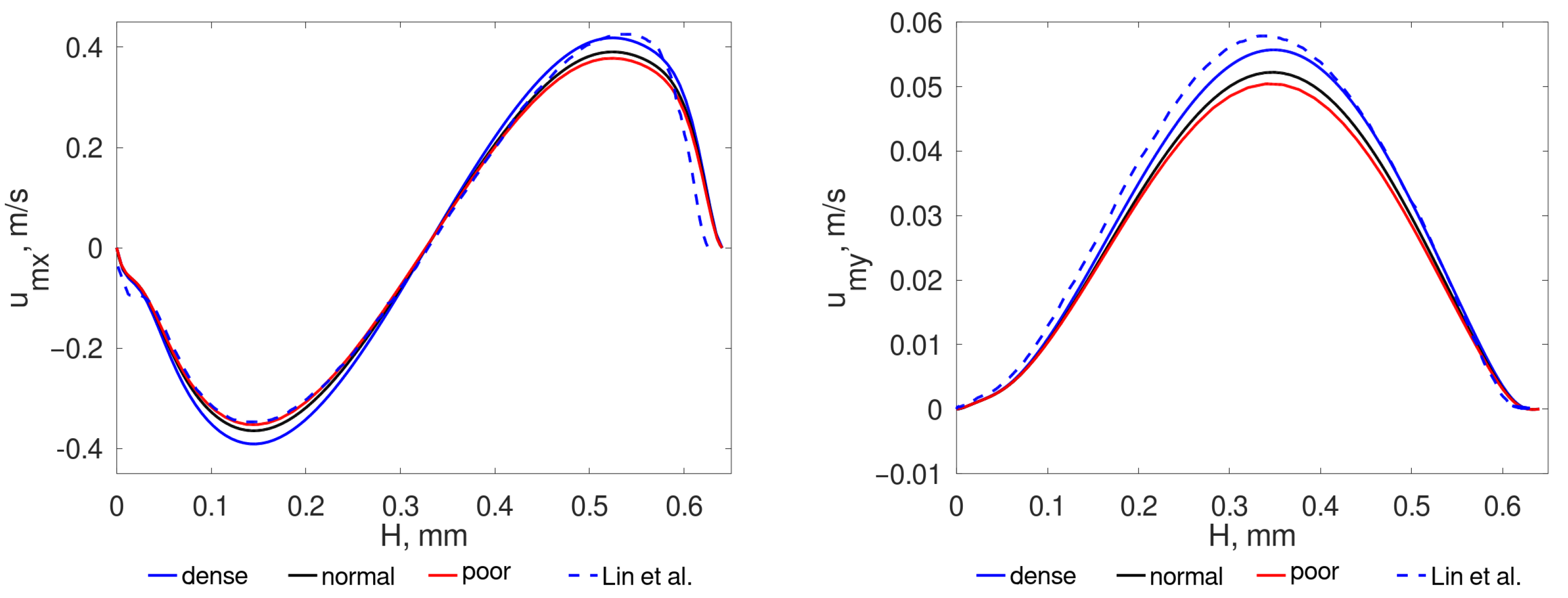
The Figure 2 shows changes of the x and y components of the streaming velocity $u_{mx}$ and $u_{my}$ for various resolutions of the mesh (cases 1A, 1B, 1C from the Table 1) and their comparison with analogous results from [4]. To perform the mesh independence study, the number of mesh elements for case 1A was increased four times (mesh 1B) and sixteen times (mesh 1C). The comparative results obtained in Figure 2 show that the compatibility with the results [4] is satisfactory for all meshes, but for further research, it was decided to choose the densest numerical mesh. It should be added that for higher frequencies and, consequently, different channel lengths and heights, the number of mesh elements was scaled relative to the 1C mesh.

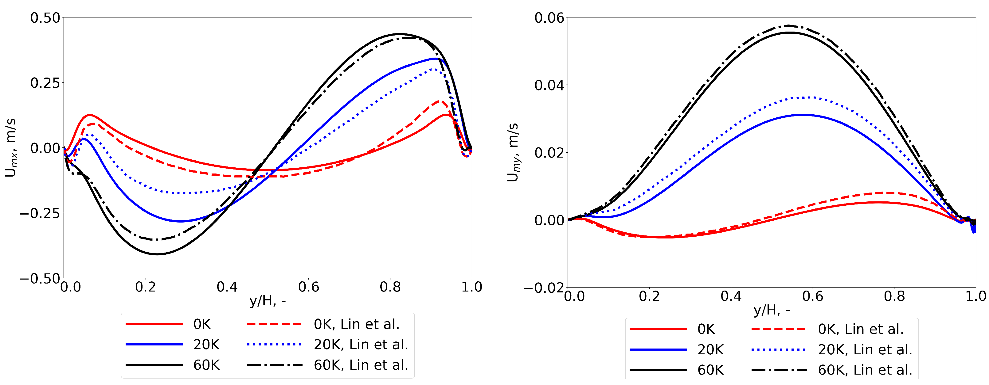
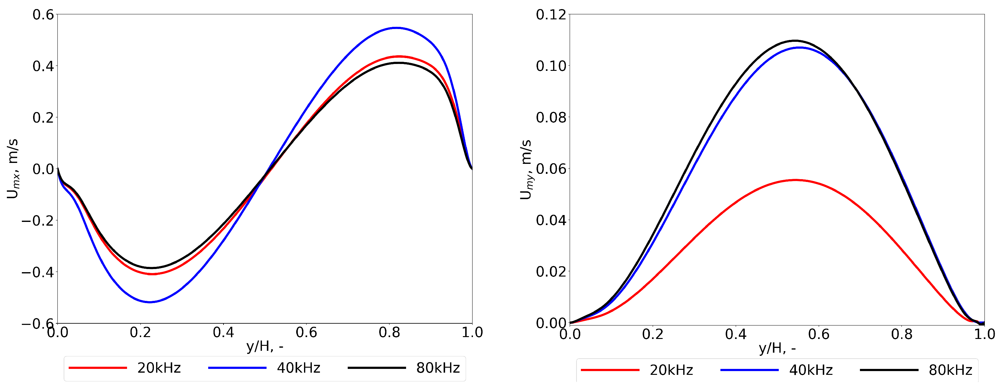
Figure 3 shows the comparison of the streaming velocity $u_{mx}$ and $u_{my}$ for various temperature difference between the top and bottom wall and their comparison with analogous results from [4].

Apart from the visible slight differences in values, the difference in symmetry of the velocity profiles seems to be more important. In general, it can be observed that the streaming velocities obtained in the current study are more symmetrical and smoother. It is more clearly visible on the instantaneous (total) velocity profiles (Figure 4).

It is important to notice that the authors of [4] explicitly stated that the FCT method may give non-physical results close to the walls.

An important conclusion from the results in Figure 3 is that the streaming velocity increases with increasing temperature difference. The maximum values of $u_{mx}$ are 0.127, 0.342, 0.436 m/s and $u_{my}$ are 0.00521, 0.0311, 0.0555 m/s for $\Delta T=(0,20,60)$ K, respectively.

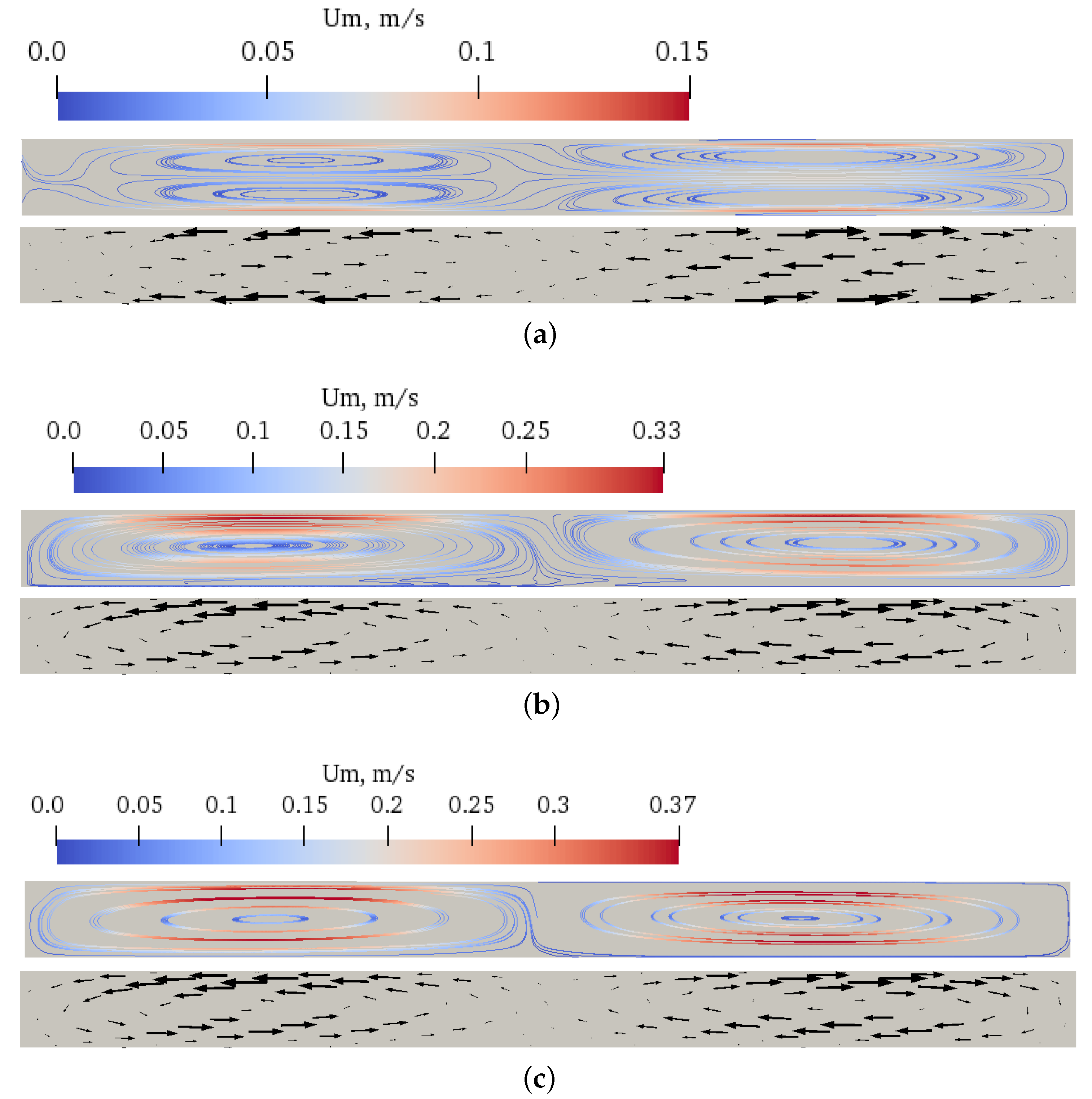
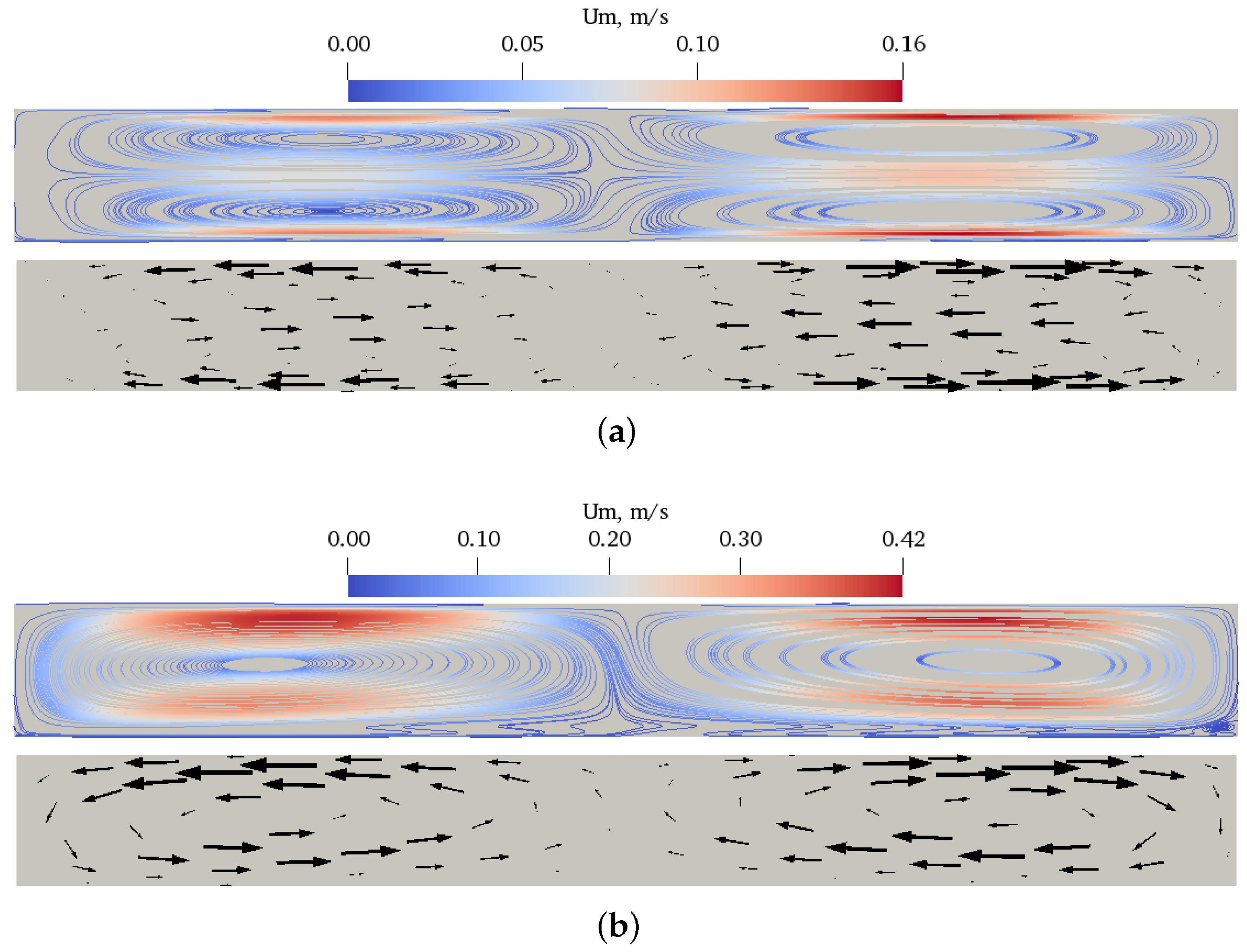
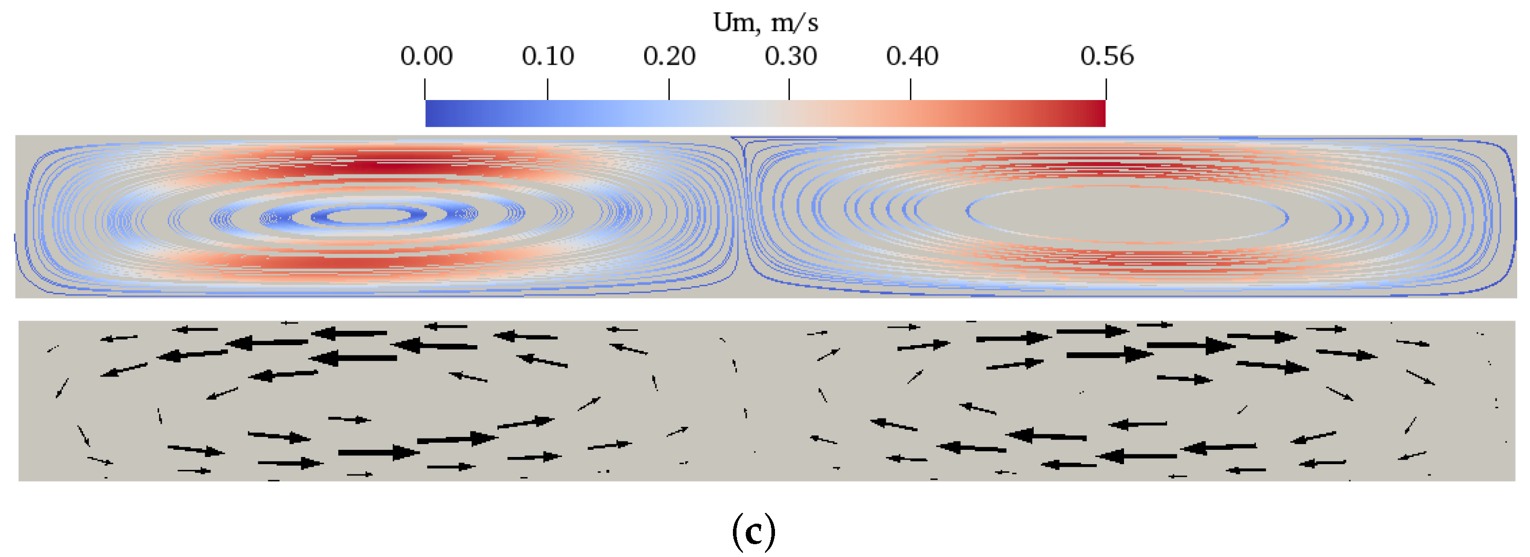
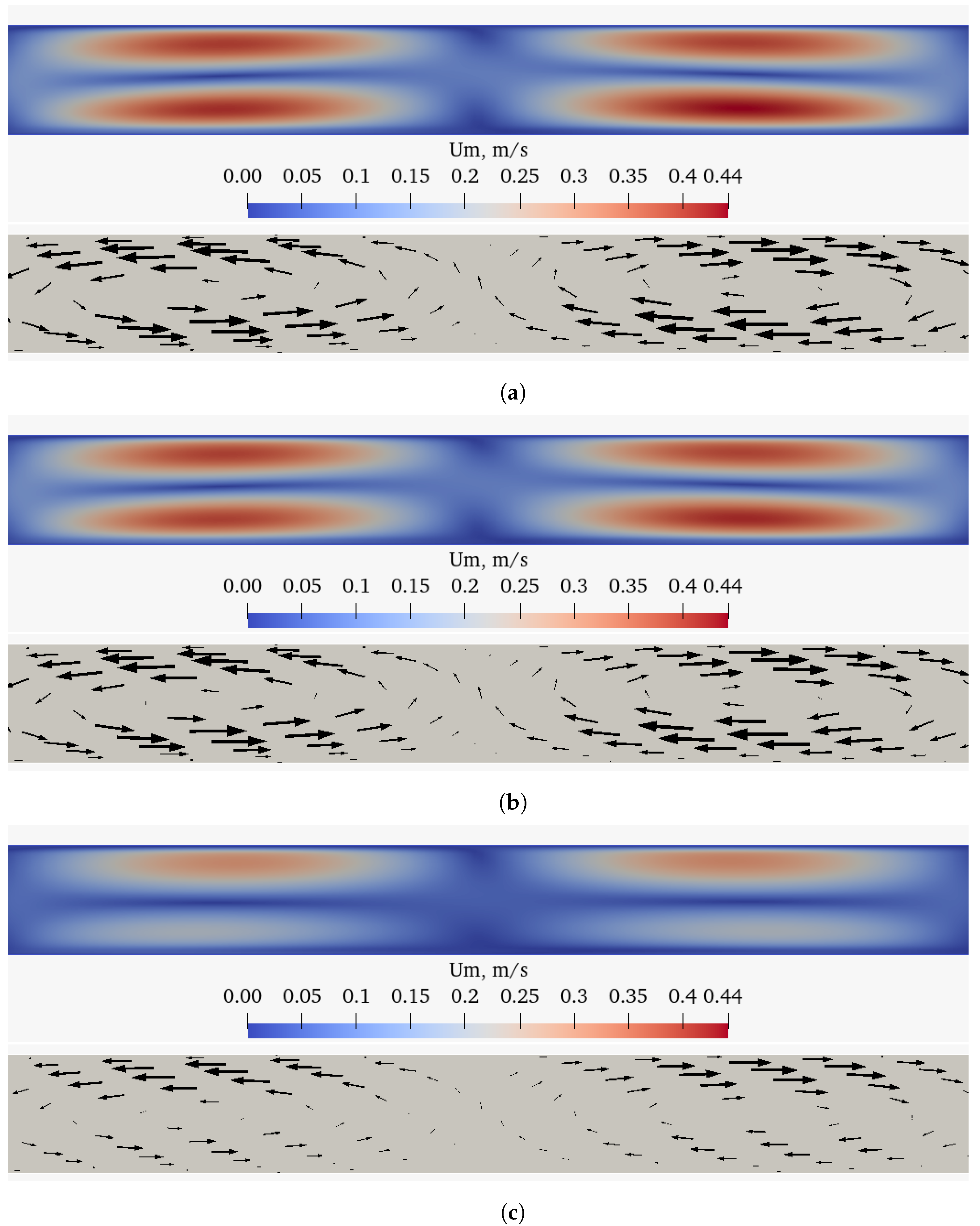
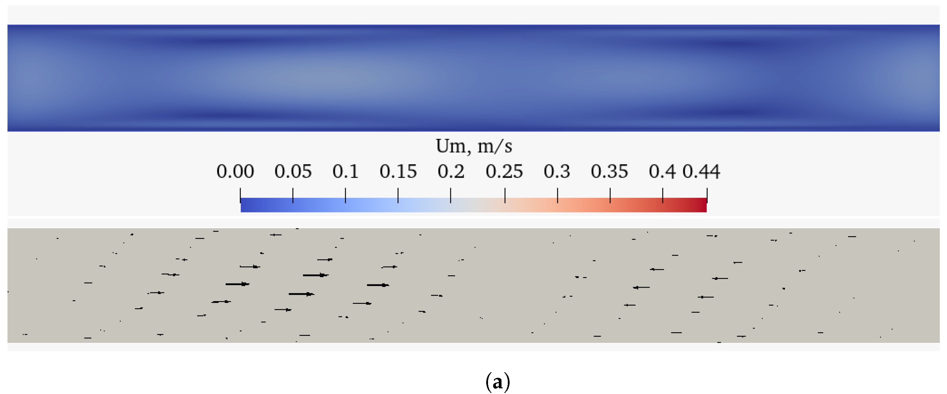
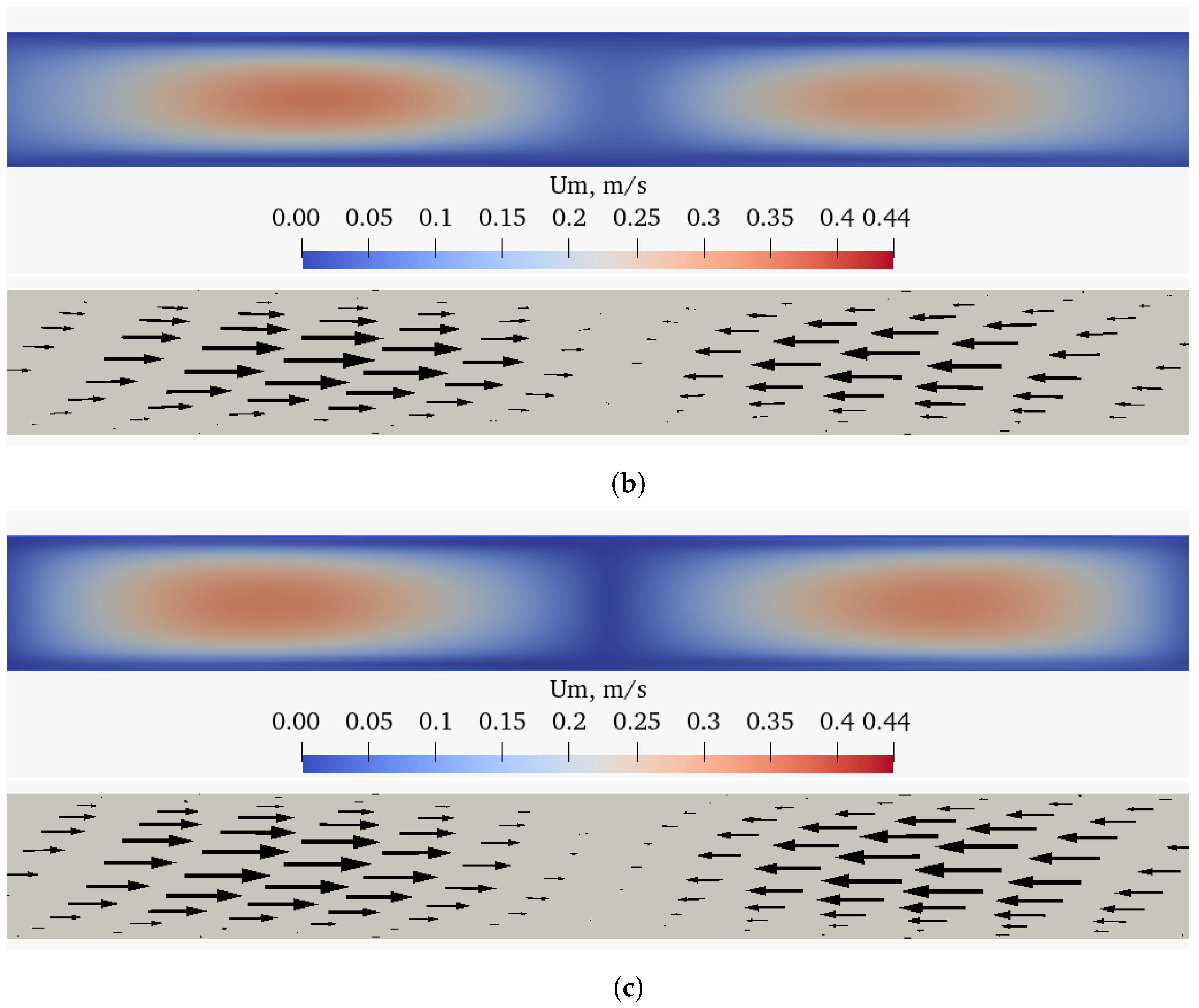
Figure 5, Figure 6 and Figure 7 show the streaming velocity vectors and streaming velocity magnitude for $\Delta T=(0,20,60)$ K and $f=(20,40,80)$ kHz. A pair of vortices rotating in the opposite direction is visible. Note that for the isothermal case $\Delta T=0$ (1A*, 2A, 3A) the vortices rotate in the opposite direction to the cases with the background temperature gradient. This is related to a different streaming creation mechanism. The isothermal streaming is driven by the vorticity production in the viscous layer and the non-isothermal streaming is produced by the baroclinic torques acting inside the flow domain. In the second case, the streaming flow and its intensity are controlled by the relative magnitudes of background density and pressure gradient [5].

With an increase in frequency from $f=20$ kHz to $f=40$ kHz, an increase of the streaming velocity was observed by about $20\%$ with maximum of $35\%$ for the temperature difference of $\Delta T=60$ K, Figure 6 c and Figure 7c. Note that although the frequency has doubled, the resulting streaming velocity has not doubled. A possible reason for this is that the channel height has decreased because its value is related to the frequency of the acoustic wave needed to create streaming. A lower channel height corresponds to a higher hydraulic resistance and therefore has a negative effect on the streaming velocity.

Note that when the frequency was increased to $f=80$ kHz the streaming velocity decreased by about $20\%$ compared to $f=40$ kHz, with a maximum decrease of $25\%$ for the temperature difference $\Delta T=60$ K. In addition, it can be seen that the temperature difference has a greater effect on the streaming velocity than the wall oscillation itself. Thus, it can be expected that the temperature difference may have a greater effect than the frequency in terms of heat transfer, although both result in a change in the streaming velocity.

Moreover, it should be noted that the Figure 5a, Figure 6a and Figure 7a show the classic Rayleigh streaming due to the presence of a viscous boundary layer. In the event of a temperature difference between the upper and lower walls, a temperature gradient is established perpendicular to the pressure gradient and a strong baroclinicity is created. The baroclinic effect is included in the Helmholtz vorticity equation as the source term $\nabla p\times \nabla \rho$ [43], causing creation of vorticity in the interior of the flow. Consequently, an emerging streaming flow does not depend on the existence of the viscous boundary layer.

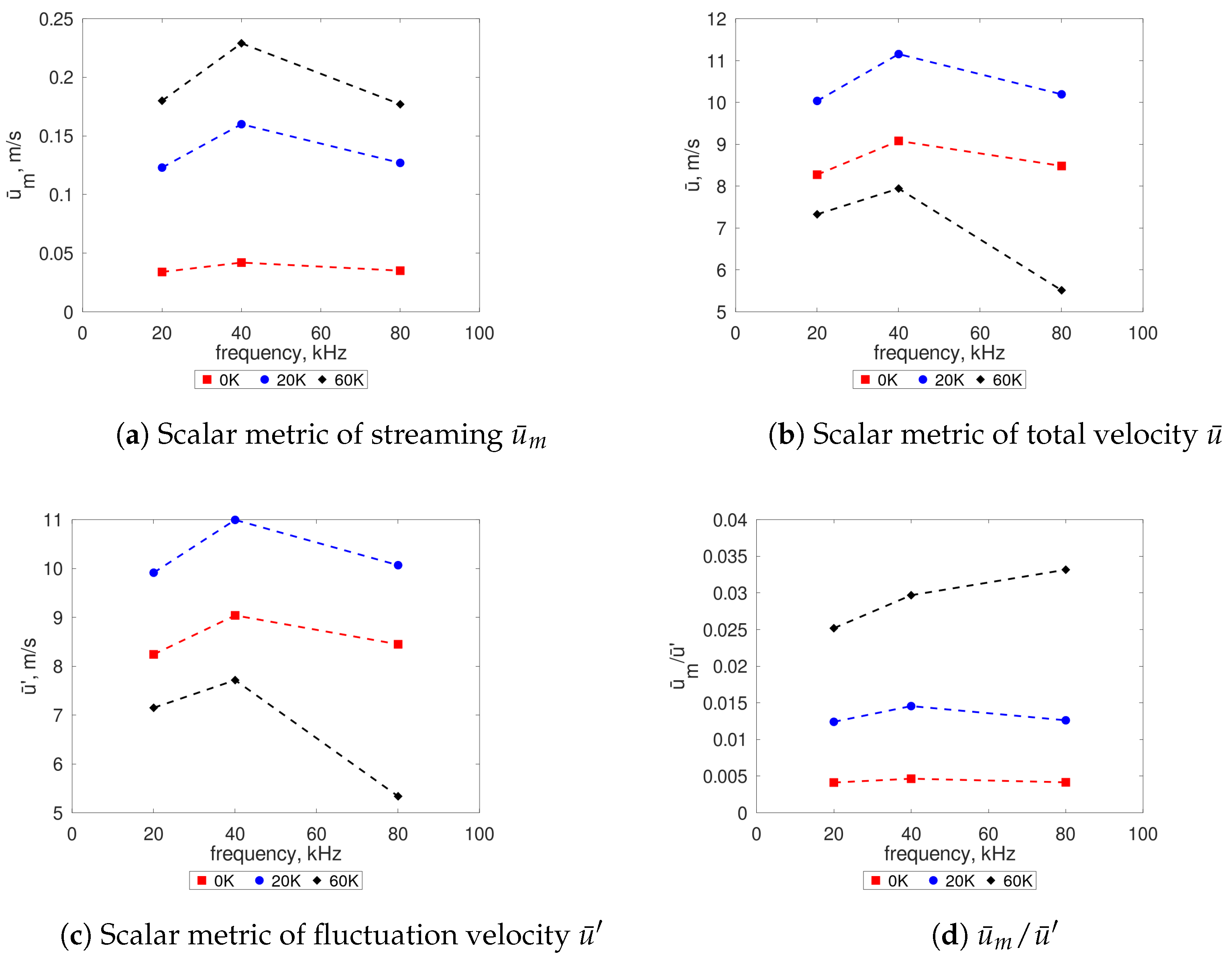
The analysis carried out in the work [5] showed that the intensity of the streaming flow should not depend on the frequency of acoustic wave. The extensive parameter space included in the present research made it possible to refer to the above statement. The Figure 8 shows the changes of scalar metrics representing the total velocity $\overline{u}$, fluctuation velocity ${\overline{u}}^{\prime }$, streaming velocity ${\overline{u}}_m$, in the function of $\Delta T$ and frequencies f. The results in the Figure 8a show that the streaming flow is only slightly dependent on the frequency of the acoustic wave and increases with an increase in $\Delta T$. Note that there is a slight maximum at 40 kHz.

Another important feature of baroclinically controlled streaming flow is its much higher intensity than classical streaming. This can be seen in the Figure 8d, where the ratio of the streaming velocity to the fluctuation velocity ${\overline{u}}_m/{\overline{u}}^{\prime }$ is presented. It can be seen that baroclinical streaming can be even an order of magnitude stronger than classical streaming.

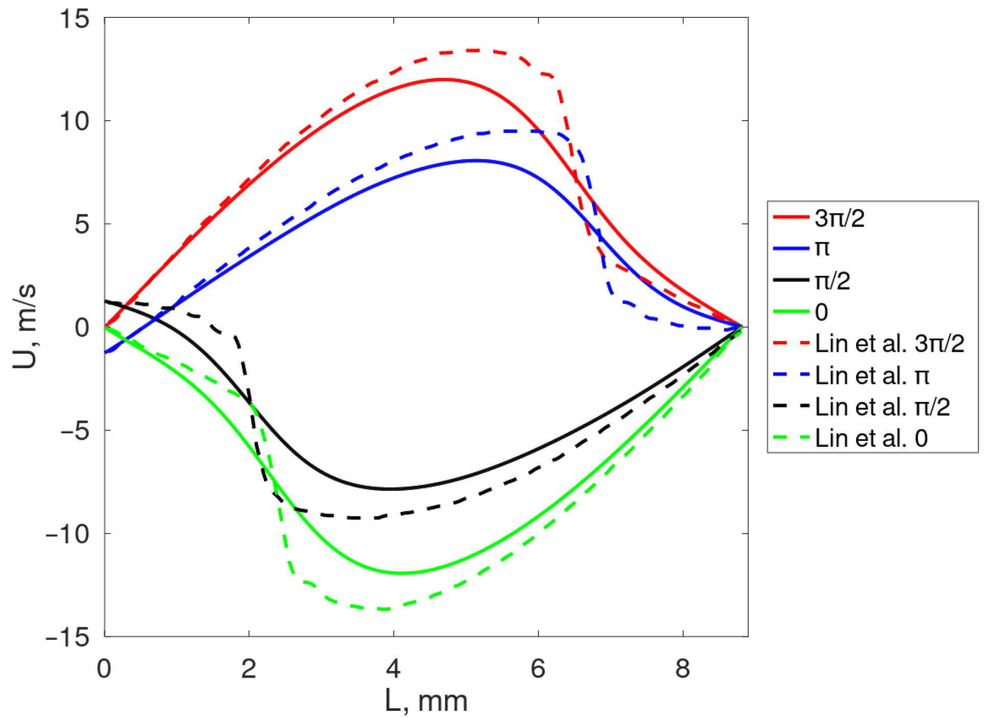
The Figure 9 shows the changes in the x component of the streaming velocity along the vertical line, starting from $x=0.75$ L for $\Delta T=60$ K. It is worth noting that the streaming reaches its maximum for $f=40$ kHz and its value for $f=80$ kHz gets very close to that for $f=20$ kHz.

A possible cause of the observable decrease in flow velocity and streaming at $f=80$ kHz may be related to the corresponding decrease in channel height H, which leads to a greater hydraulic resistance in the channel. This points to another possible research direction, the study of the influence of the channel height on the streaming flow.

4.1. Impact of the Third Dimension on the Streaming

Three-dimensional calculations were performed for the case 2C characterized by the frequency $f=40$ kHz of the oscillating wall and $\Delta T=60$ K. The width of the 3D resonator W was equal to its height. The resolution of the mesh and its structure in the width direction was the same as in the height direction, resulting in a 150 × 180 × 180 mesh giving 4,860,000 mesh cells. The boundary walls in the width direction were assumed to be no-slip and adiabatic.

The main motivation to perform the full 3D calculation of one of the studied cases was to compare it with its 2D counterpart and to observe the effect of bounding adiabatic walls on the acoustic streaming. It should be noted that the 3D calculations were very time-consuming and their performance for the entire range of parameters included in the current research was beyond the scope of this study.

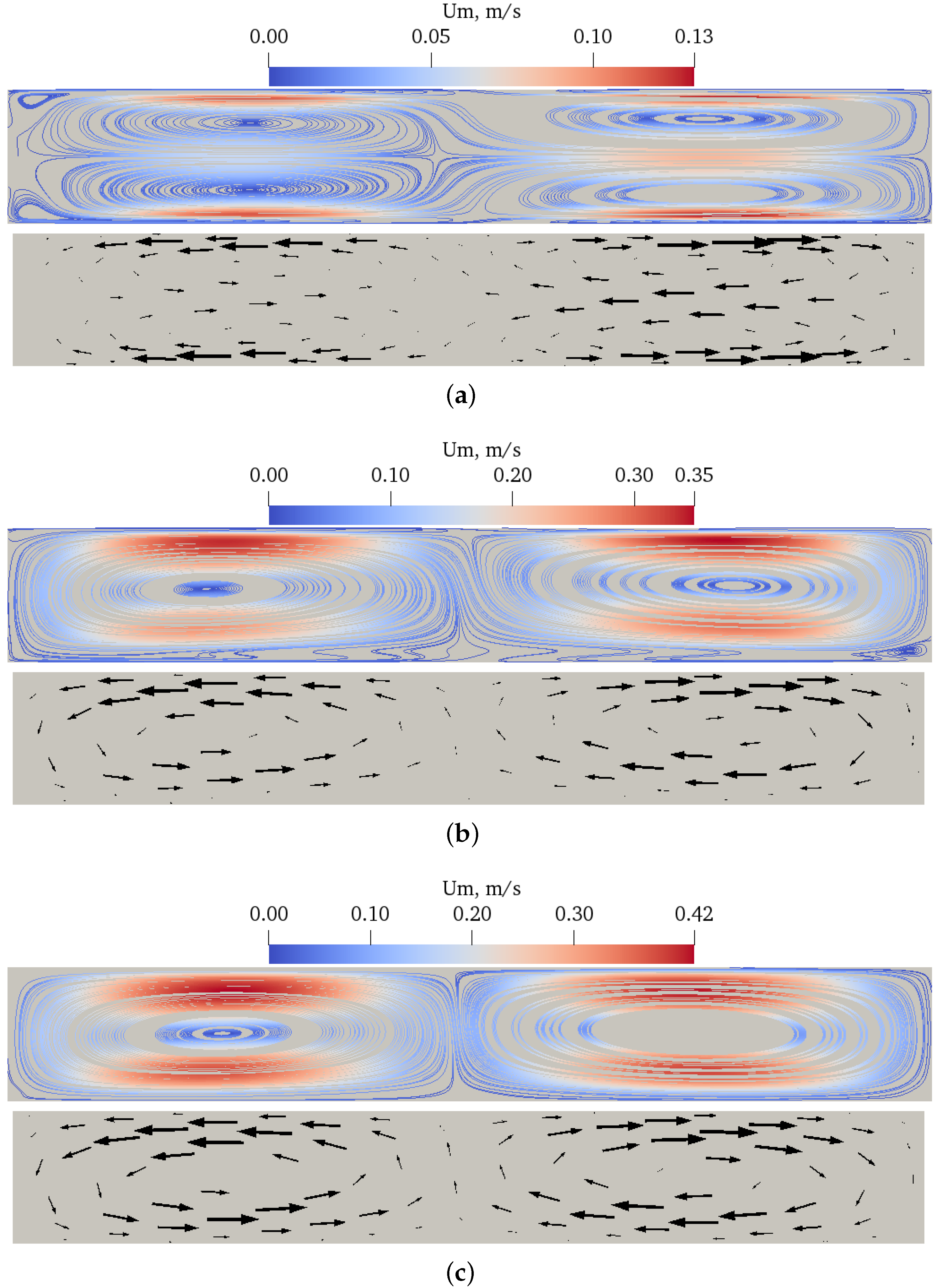
The 3D streaming flow was examined in a number of 2D longitudinal cross-sections taken along the height and width direction of the resonator. The cross-sections were taken at $z=(0.05$, $0.125,$$0.25,$$0.375,$$0.5,$$0.625,$$0.75,$$0.875,$$0.95)$ W and $y=(0.05,$$0.125,$$0.25,$$0.375,$$0.5,$$0.625,$$0.75,$$0.875,$$0.95)$ H creating $xy$ planes and $xz$ planes respectively. The Figure 10 and Figure 11visualize the established streaming flow in the cross-sections at $z=(0.125,$$0.375,$$0.5)$ W and $y=(0.125,$$0.375,$$0.5)$ H respectively. Note that the streaming flow patterns established in the $xy$ planes are symmetrical in respect to the $z=0.5$ W plane, but unsymmetrical in the $xz$ planes, and after crossing the resonator center ($y=0.5$ H) the flow direction on the $xz$ planes is reversed. This is fully related to the direction of rotation of the 3D streaming vortices.

By examining the 2D cross-sections of the streaming (Figure 10a–c), it can be seen that the structure of the vortices is preserved, but their intensity decreases approaching the wall.

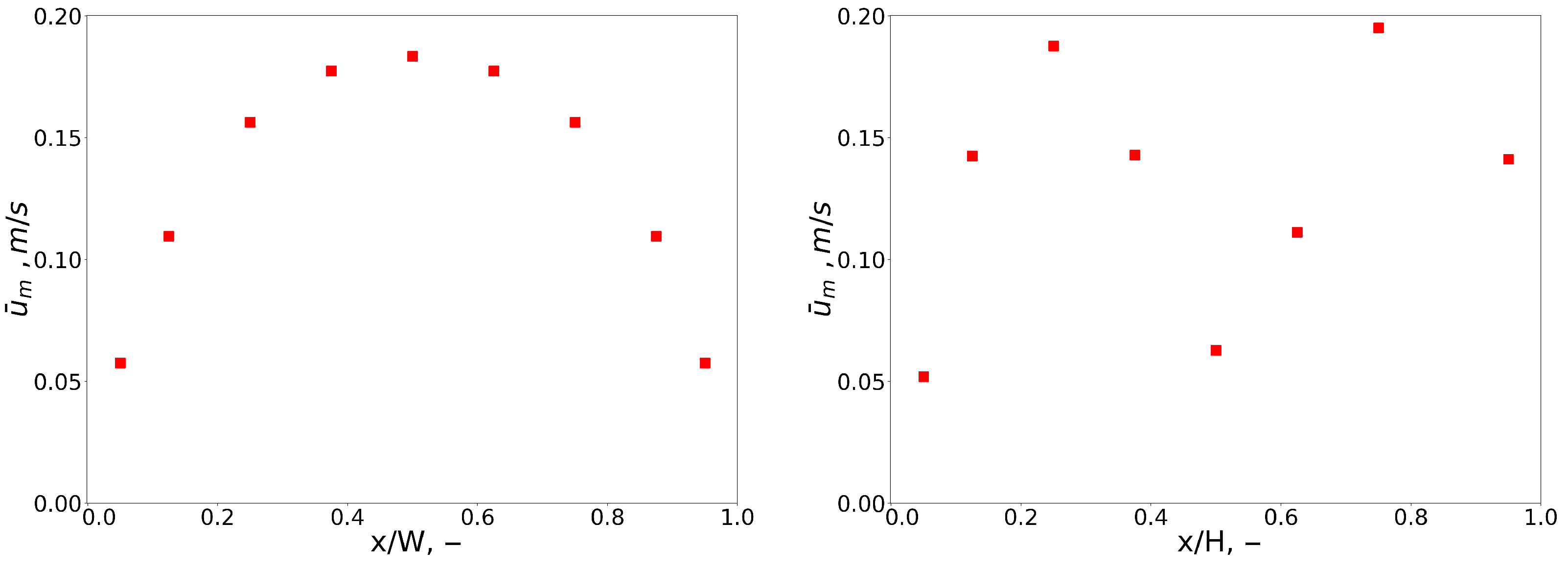
Figure 12 shows the scalar metric of the streaming flow calculated in each considered cross-section according to the Formula (10). On the left graph of the Figure 12 it is clearly visible that the streaming weakening towards the wall is not linear, but rather quadratic. It is worth adding that the scalar metric of the streaming intensity creates a quasi-parabolic profile along the width of the resonator.

Scalar metrics computed for the $xz$ planes along the height of the resonator are shown in the right-hand plot of the Figure 12. Their values are related to the magnitude of the streaming velocity in the corresponding $xz$ plane and illustrate the vortex topology. The two visible peaks shows the positions of the largest longitudinal velocities of the streaming. Note that the maximum at $y=0.875$ H is higher than this at $y=0.25$ H, which shows that locally the velocities at the top of the streaming are greater than those at the bottom. This is also seen in Figure 10.

4.2. Impact of Streaming Flow on Heat Transport

The

Table 2. Nusselt number at the top and bottom wall.

Case	$\Delta \mathit{T}$, K	f, kHz	${\mathit{Nu}}_{\mathit{top}}$	${\mathit{Nu}}_{\mathit{bot}}$
1B*	20	20	1.321	1.258
1C*	60	20	1.239	1.221
2B	20	40	0.856	1.305
2C	60	40	1.015	1.241
3B	20	80	0.640	0.941
3C	60	80	0.752	0.887

shows the mean Nusselt numbers for the top and bottom walls of the considered channels and the flow parameters. For the acoustic wave frequency $f=$ 40 kHz and $f=$ 80 kHz, the Nusselt number ($Nu$) is generally smaller compared to the cases for $f=$ 20 kHz. Changing the frequency from $f=$ 20 kHz to $f=$ 40 kHz for $\Delta T=20$ K caused the Nusselt number to drop $35\%$ for the top wall and an increase of $3.7\%$ for the bottom wall. For $\Delta T=60$ K, the Nusselt number on the top wall decreased by $18\%$ and increased by $1.7\%$ on the bottom wall. The increase from $f=40$ kHz to $f=80$ kHz for $\Delta T=20$ K caused a further decrease of the Nusselt number by $25\%$ for the top wall and $28\%$ for the bottom wall, and for $\Delta T=60$ K the Nusselt number decreased by $26\%$ for the top wall and by $24\%$ for the bottom wall.

Note that the Nusselt number is influenced by the distance between the heat transfer surfaces, see Equation (15). If this distance is reduced, the effect of conduction increases, and if the distance increases, the effect of convective heat exchange increases. In the present study, the frequency and height of the channel were related with the relationship (1). Consequently, as the frequency increased, the channel height decreased. This could have had a significant impact on the obtained values of the Nusselt number. It is worth noting that, as in the case of the intensity of the acoustic streaming as a function of frequency (Figure 8a), a change in the channel height may indicate the existence of an optimal frequency for which the value of $Nu$ is at its maximum. It seems that it is worth extending the existing research to include the research on the impact of changes in height and to confront such results with the analysis carried out in [35].

The greatest change in the mean Nusselt number occurred with an increase in frequency from $f=$ 20 kHz to $f=80$ kHz, for the temperature difference $\Delta T=$ 20 K. In this case, the mean Nusselt number decreased by $51.6\%$ on the top and by $25.1\%$ on the bottom wall. For the temperature difference $\Delta T=$ 60 K, the mean Nusselt number decreased by $39.3\%$ and $27.4\%$ for the top and bottom walls, respectively.

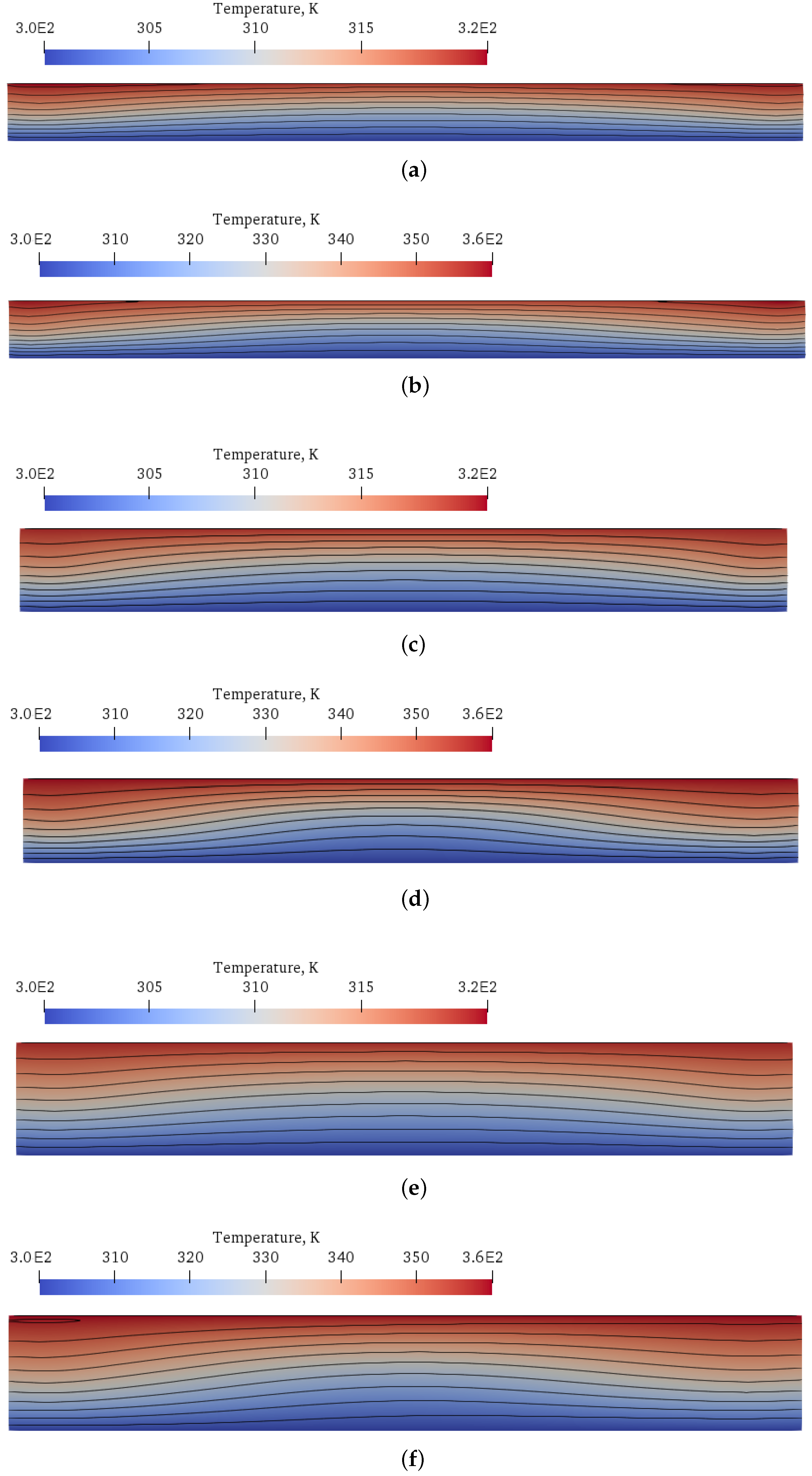
Figure 13 shows cycle-averaged temperature maps, calculated analogically to the streaming velocity $\overline{u}$, for the frequencies f = 20 kHz, f = 40 kHz and f = 80 kHz. The irregular distribution of the mean temperature gradient in the flow domain can be observed. It can be seen that the highest temperature gradient is established close to the bottom corners and near the top wall at the centre of the channel.

The high gradients of the mean temperature are closely related to the intensity and topology of the streaming flow, compare with the Figure 5, Figure 6 and Figure 7. In the middle section of the channel, the streaming velocity is pointed upwards and at the side walls is directed downwards, intensifying the heat transport between the top and bottom walls. Similar distribution of the mean temperature is observed for all considered frequencies and not surprisingly the temperature gradients are stronger for the flows with $\Delta T=60$ K.

It is worth noting that the increase in temperature difference between the top and bottom walls did not cause the increase in the mean Nusselt number. It can be explained by the hypothesis that the increase in convective heat transfer, related to the streaming, was equalized by the increase in conductive heat transfer between the fluid layers.

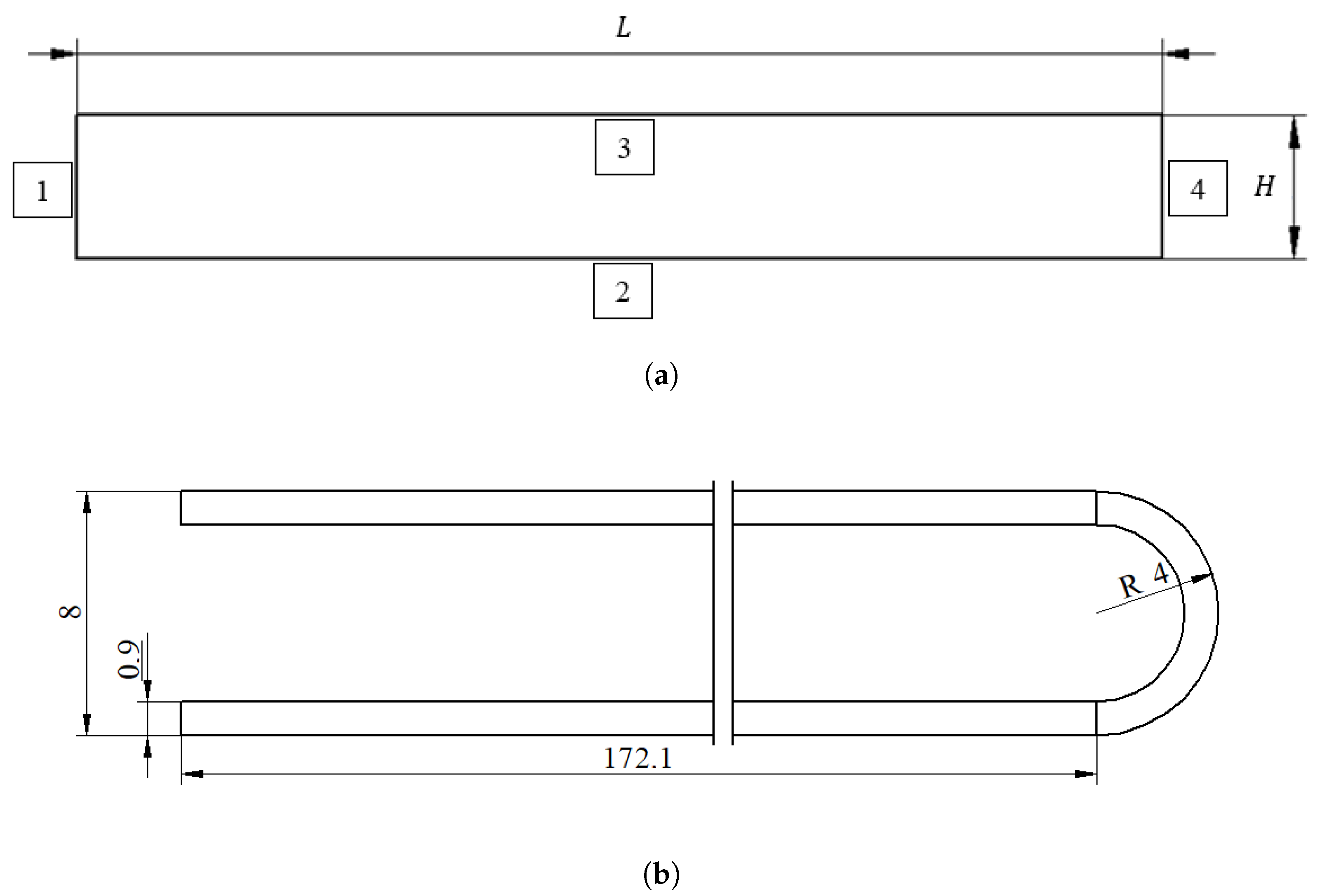
4.3. Application of Streaming Phenomenon in Pt-100 Resistance Thermometer

Based on the following study, an analysis of the acoustic streaming was carried out in Pt-100 resistance thermometer from the Figure 1b. It should be noted that the geometry of the thermometer under consideration is characterized by long and narrow channels and that the streaming flow is induced by the oscillation of its far end and short vertical wall.

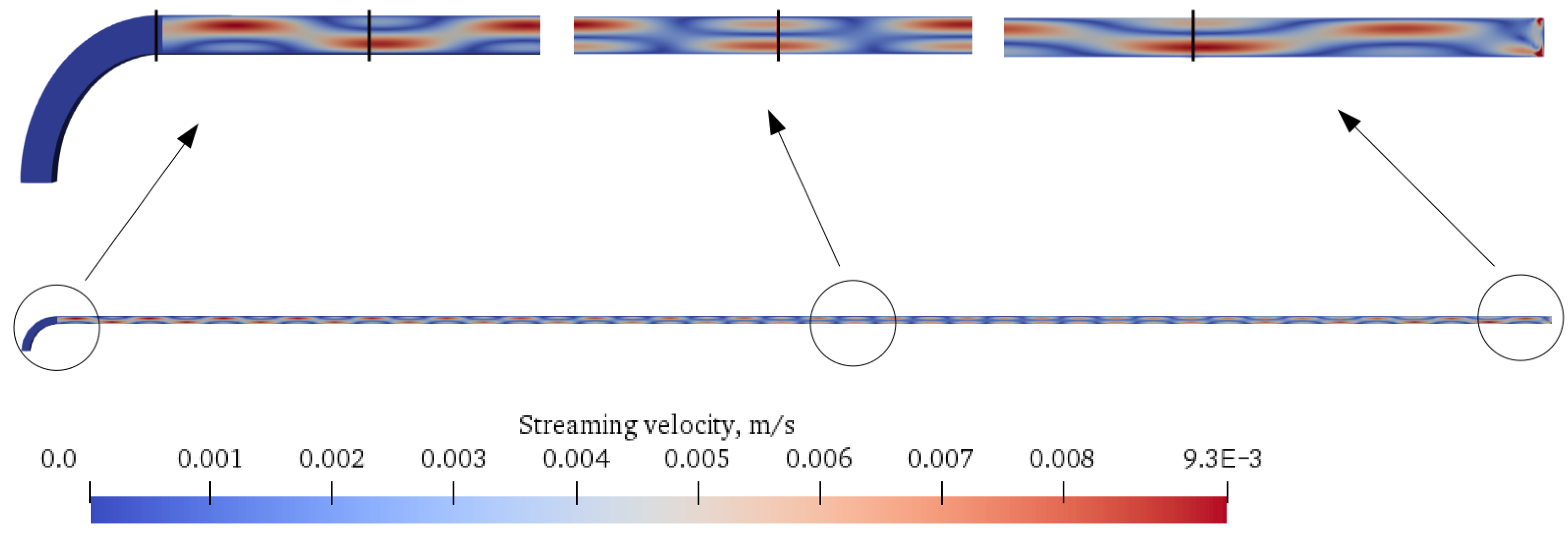
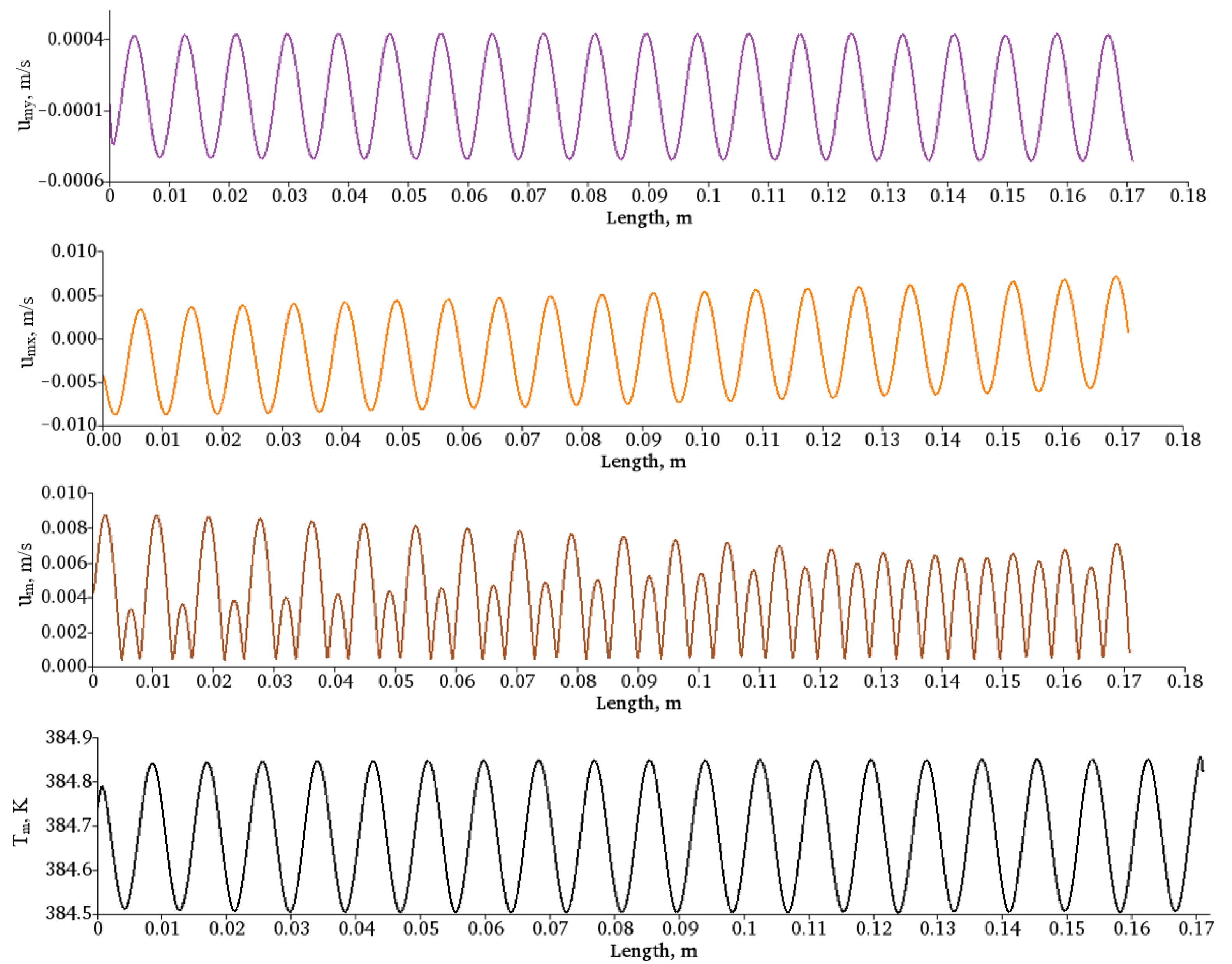
The Figure 14 shows the streaming velocity magnitude. The streaming vortices are clearly visible along the air-filled channel of the thermometer. It should be noted that the streaming adjusted itself to the height and length of the thermometer resulting in a row of consecutive vortices.

Figure 15 shows the changes of vertical component of the streaming velocity ${\overline{u}}_y$, horizontal component of the streaming velocity ${\overline{u}}_x$, the magnitude of streaming velocity $\left|\overline{\mathbf{u}}\right|$, and the mean temperature $\overline{T}$ along the thermometer channel taken at the height $y=0.825$ H. The graph presenting the course of the velocity ${\overline{u}}_y$ shows that there are 20 pairs of counter-rotating vortices of similar strength along the channel. On the basis of the graphs showing the course of ${\overline{u}}_x$ and $\left|\overline{\mathbf{u}}\right|$, it can be noticed that the vortices rotating clockwise weaken as you move away from the oscillating wall, while anticlockwise vortices behave in the opposite way. It can be see that the peak velocity has changed from ${\overline{u}}_x=0.0071$ m/s to ${\overline{u}}_x=0.003$ m/s.

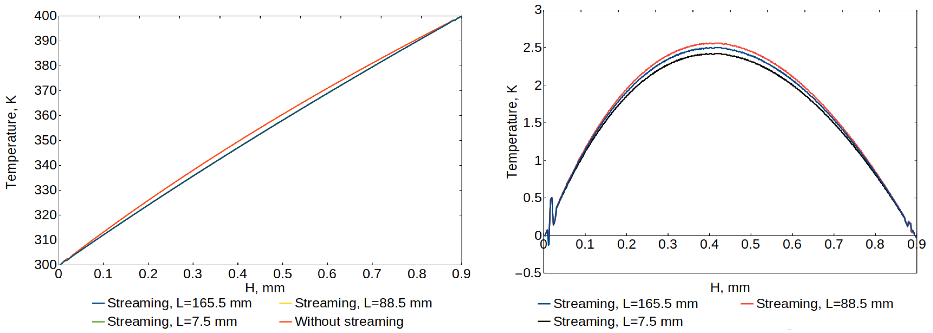
The Figure 16 shows the cycle-averaged temperature profiles established in the thermometer channel at 3 different locations $x=(7.5,88.5,165.5)$ mm and compares it with the flow without streaming. To better illustrate the differences between the flow with and without streaming at the selected locations, the temperature differences between the temperature profiles of the flow with and without streaming are also shown (left graph of the Figure 16). It can be observed that the greatest difference, slightly above 2.5 K, occurs at $x=7.5$ mm (near the oscillating wall), and the smallest difference, still above 2 K, occurs at the center of the channel $x=88.5$ mm. Interestingly, the temperature difference starts to increase again as moving away from the center of the channel and is larger at $x=165.5$ mm than at $x=88.5$ mm. Moreover, the maximum temperature difference is approximately halfway up the channel height for all considered locations.

Summarizing, it can be stated that, as in the case of the basic, short rectangular geometry, one vortex fills the entire height of the channel, but due to the considerable length of the channel, the vortices approaching the left non-oscillating wall have less regular shapes. Moreover, the fluid movement caused by the high amplitude acoustic streaming intensifies convective heat transfer and a shortening of the measurement time of the thermometer can be expected.

5. Conclusions

This work focuses on the numerical study of large-amplitude, acoustically-driven streaming flow for the frequency range of the acoustic wave from 20 kHz to 80 kHz and temperature differences $\Delta T=(0,20,60)$ K between hot and cold surfaces. The geometries studied include two-dimensional rectangular resonators of various lengths, one three-dimensional rectangular resonator, and one long and narrow channel, representing a typical U-shaped resistance thermometer.

The mathematical model is based on the Navier–Stokes compressible equations and the ideal gas assumption. The numerical model is based on the finite volume method, and the computations are carried out with the use of OpenFoam CFD libraries. The desired frequency acoustic wave is created by vibrations of one of the walls of the considered geometry, which is modeled as a dynamically moving boundary of the numerical mesh.

The proposed numerical methodology is validated by comparison with the high-order numerical method used in [4]. Consequently, it turns out that the relatively low-order but fast and flexible FVM method captures the demanding and multiscale dynamics of compressible fluids over time scales, from the acoustic wave period to the slow time scale over which the streaming flow evolves. This shows that the FVM method can be successfully used in the study of streaming phenomenon in complex geometries and can be a good predictive tool for designing experiments.

Simulations in 2D resonators confirm that the baroclinic acoustic streaming is largely frequency independent, and its intensity increases with the temperature gradient between the hot and cold surface. It can be potentially important that a slight maximum of the streaming flow is observed at 40 kHz, which may suggest the optimal frequency of the acoustic wave for a specific application. This maximum also varies weakly with the temperature gradient. This suggests that the streaming phenomenon may have an even more positive effect in the case of large temperature differences between hot and cold sources and that the frequency of the acoustic wave should be selected in accordance with the expected temperature difference.

Simulations in a 3D resonator show that a three-dimensional pair of streaming vortices is formed in the whole space of the resonator. Examination of the streaming flow in the longitudinal cross-sections exposes that the intensity of streaming is gradually decreasing approaching the side walls of the resonator creating a quasi-parabolic profile. It shows that the future development of this research should focus on fully 3D calculations for various frequencies and temperature gradients and a precise identification of the influence of the bounding walls on the streaming flow.

Simulations in the long and narrow channel, the dimensions of which corresponded to a typical U-shaped resistance thermometer, show that the acoustic streaming can be induced by vibration of the far end vertical wall and manifest itself as a long row of counter-rotating vortices that vary slightly along the channel. Moreover, comparing the simulation with and without wall vibrations shows that the movement of the fluid caused by the acoustic streaming flow intensifies the convective heat transfer, which may shorten the measurement time of such a thermometer.