1. Introduction
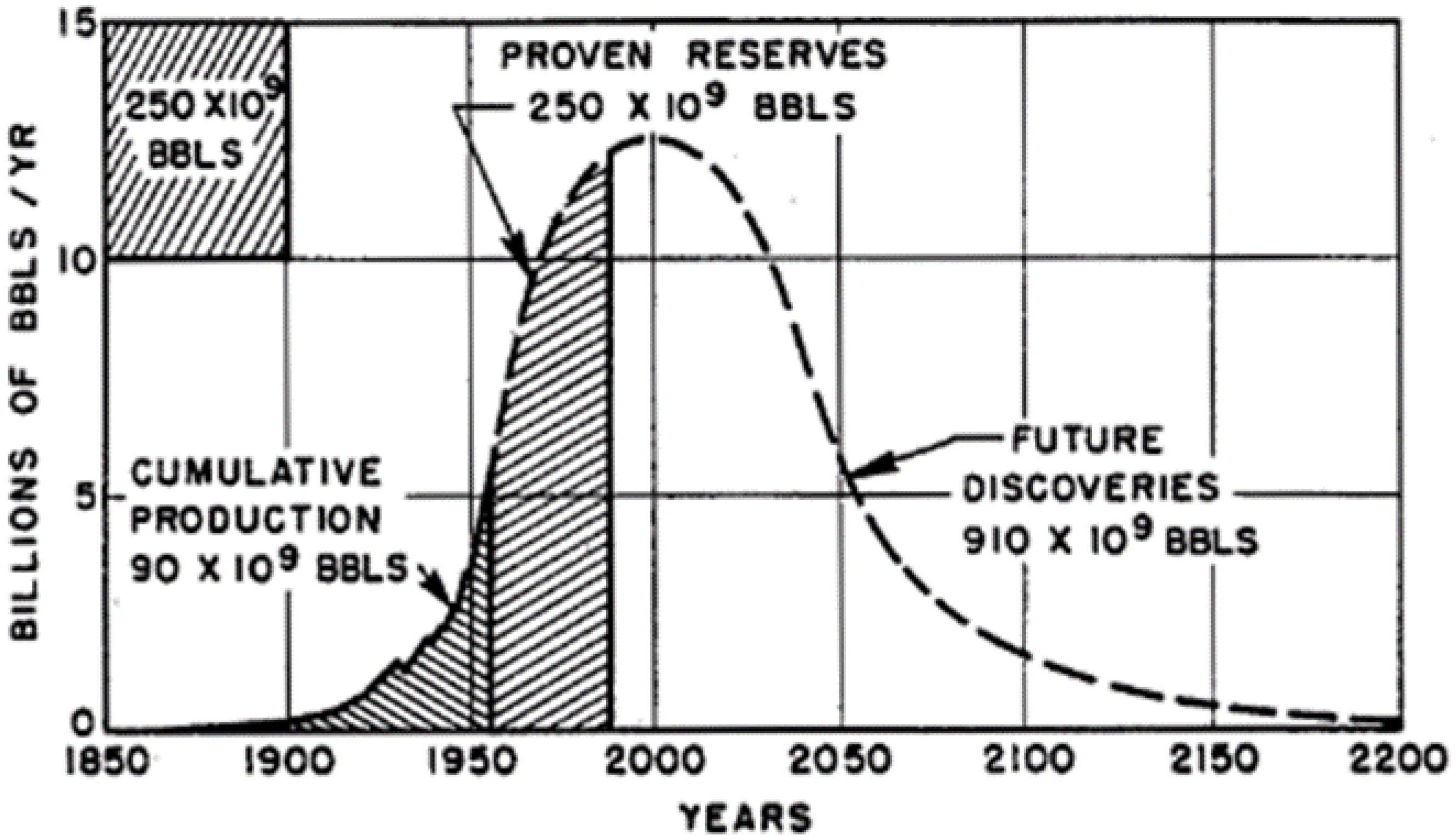
Hubbert [
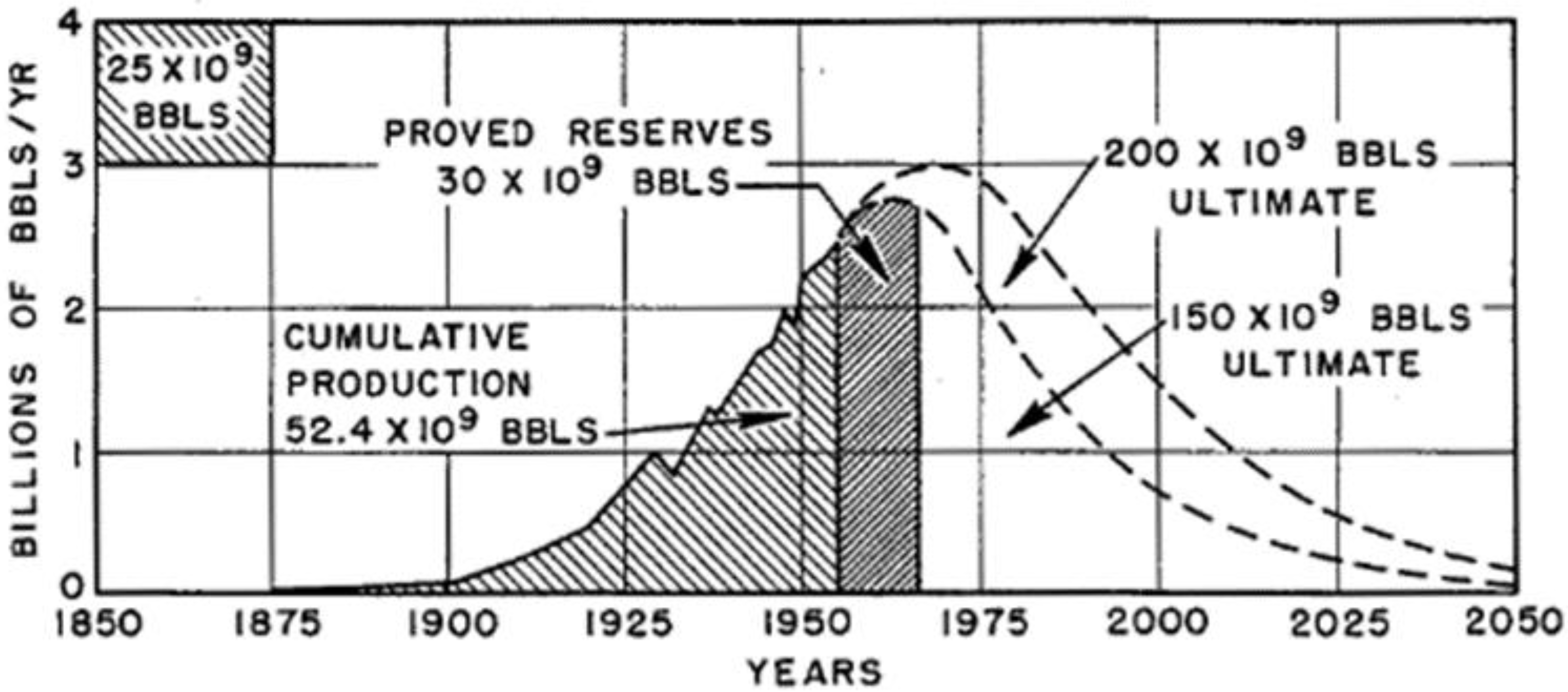
1] proposed a production rate curve under the assumption of scarcity for oil. The assumption of depletion is clearly stated since there is an initial fixed supply and the demand will exhaust it. Moreover, the curve for all the depleted resources has a certain course. Production rates start slowly and then rise extremely steeply until the peak. From the moment they peak, then they follow again a steep decline. Under Hubbert’s calculation, the maximum production rates will be reached at about 2000 (year). We present the two production curves (original from Hubbert’s research) with a single peak for global and US production in
Figure 1 and
Figure 2 [
2]. The issues of energy security and energy transition are also raised from these assumptions. Hubbert recognizes that national security issues are stemming from an energy security perspective since domestic US supply will not be able to cover demand. Moreover, if hydrocarbons are depleted before an efficient energy transition, prices for the remaining resources will climb while the climate crisis will be exacerbated. On the contrary, if oil is not suddenly depleted, and soon, then a lock-in in hydrocarbons might prevail prolonging hydrocarbons’ exploration. We test the hypothesis of depletion by researching whether a single peak will exist or existed. This will also determine the rate of energy transition and its timing.
These calculations initiated a whole new field of research. Geologists and economists have numerously tried to detect when and at what level oil production will peak. Oil was long conceived as a commodity in scarcity and its overconsumption by one generation would cause intergenerational imbalances. If the depletion comes sooner than the energy transition, then an economic downfall will follow. Hotelling [
3] proposed that the fossil fuel price with the marginal cost subtracted will increase to the levels of interest rates as depletion continues. However, for his results to hold, the assumptions of perfectly competitive markets and that of no information asymmetries should be satisfied. These assumptions are difficult to be satisfied all the time and across all markets. Moreover, the extraction rates determine current consumption. Firstly, Hubbert’s curve follows a symmetric logistic distribution. It remained unclear when Peak Oil would occur around the 1970s in the US and how high total production would be. Campbell and Laherrere [
4] went on with their updates over reserve forecasts. This research calculated that Peak Oil would be reached between 2004 and 2006, and then a production decrease would follow. Campbell [
5] should be accredited with the term “Peak Oil”. Peak Oil is the point when extraction rates of a depleted resource reach their maximum. Consequently, extraction returns were restrained by geological conditions. However, there is a hesitation by many linking Peak Oil with depletion. Gradual depletion increases extraction costs. Factors such as demand growth, technological advancements, increased inventories, and site development can increase production and supply and strengthen consumption. Many propose that depletion will not be a concern in the future (Dale and Fattouh [
6]). They propose that oil passed from the era of scarcity to that of abundance due to technological evolutions. Unconventional production poses a serious argument to the theory of Hubbert’s curve. Mardashov et al. [
7], Zhao et al. [
8], and Zheng and Sharma [
9] provide a series of late technological advancements which increase oil exploitation and decrease costs.
The start of the unconventional revolution dates to the mid-20th century when Stanolind Oil and Gas (a subsidiary of Amoco) experimented with the fracturing technique in Kansas using gelled gasoline and sand from the Arkansas river [
10]. Multi-stage hydraulic fracturing in combination with horizontal drilling (60 years later) set the shale oil and gas revolution in the US. Unconventional production is an easily available and low-cost exploration process in the US. Apart from the technological advancement of shale, the market is extremely interesting regarding its structure. The energy sector is primarily regulated by the Federal Energy Regulatory Commission (FERC). Interestingly, the hydrocarbons sector is within the authority of eight other offices and authorities that oversee specific components. The total number of regulatory authorities is 9, something which might be deemed as complex [
11]. While the regulatory bodies are sufficient, [
12] clearly states in the Government Policy Objectives that “The US Government does not have a national energy policy”. On the contrary, in the same sector for 2020, [
13] states that now the Federal policy supports the activities of oil and gas production. The two different policies objectives show how the market and technological evolutions changed the structure of the energy sector. The US regulatory status changed in December 2015 when the exports ban was lifted. Since then, exports increased tenfold from 100,000 bpd to 1.086 million bpd in 2019. While one would expect the large numbers of regulatory bodies and the meteoric change of the US oil market alteration from a net importer to an exporter to have required a vast federal regulatory change; this does not hold. In [
13], it is stated that oil production is regulated by each state separately and this varies a lot, while pipeline construction is federally regulated only when it crosses borders. Finally, multiple state offices can also have jurisdiction over the construction and operation of pipelines crossing different states. Moreover, [
14] clearly states that federal regulation has more to do with environmental issues. Further, [
12] clearly describes that the US domestic market is dominated by private contracts. As the aforementioned suggest, production rates and exploration activities are primarily driven by corporate decisions and available technology. The different states have different regulations, and private production is the mainstream. Oil production and rates are not regulated by a body. This is the reason why we report our research for each different region and not in total. Federal regulation comes in the downstream section where oil has to be transported and stored or exported. Thus, this might explain some of our results since production rates and downstream utilities are determined by corporations and federal bodies, respectively. The different nature and incentives between the market actors (corporations and regulatory bodies) might cause downstream imbalances or distribution bottlenecks.
Our null hypothesis is that if the Hubbert curve holds, then oil production rates should have or are in the process of experiencing a single peak. Hubbert’s curve is a model of a single maximum. If the alternative holds, then oil production rates are not determined by reserve quantities but by other drivers. Thus, oil is not a resource in scarcity whose extraction rates will reach a single maximum if producers compete to extract as much in the shortest period. Multiple extraction rate peaks will verify the alternative hypothesis which will be of different reasoning from Hubbert’s curve. This is why we apply the tests and date stamping processes from the asset pricing field to detect periods of exploratory exuberance. If multiple periods of such explosiveness exist, then our tests reject the null of depletion for oil since there will be times when productivity will experience bursts.
The objective of this paper is to research the essence of a single peak in oil productivity and thus the whole curve and shed light on long-lasting perceptions. If Hubbert’s production model is verified, then the peak production has passed or we are near the peak and then the global economy is threatened by the resource scarcity and price skyrocketing since there will be no available quantities in the long term. However, if the production curve does not hold, then oil lock-in will continue supplying the global economy with adequate quantities in the future. This will postpone energy transition and oil extracted in sufficient quantities at low prices will exacerbate climate change. Furthermore, altering production rates may cause significant volatility in the commodity markets since supply will respond to demand signals with a lag. Issues like energy security, energy transition, and market design are of great interest for policymakers. For all of the above, we consider our effort to research the field as significant. We apply the Phillips et al. [
15] and the Phillips et al. [
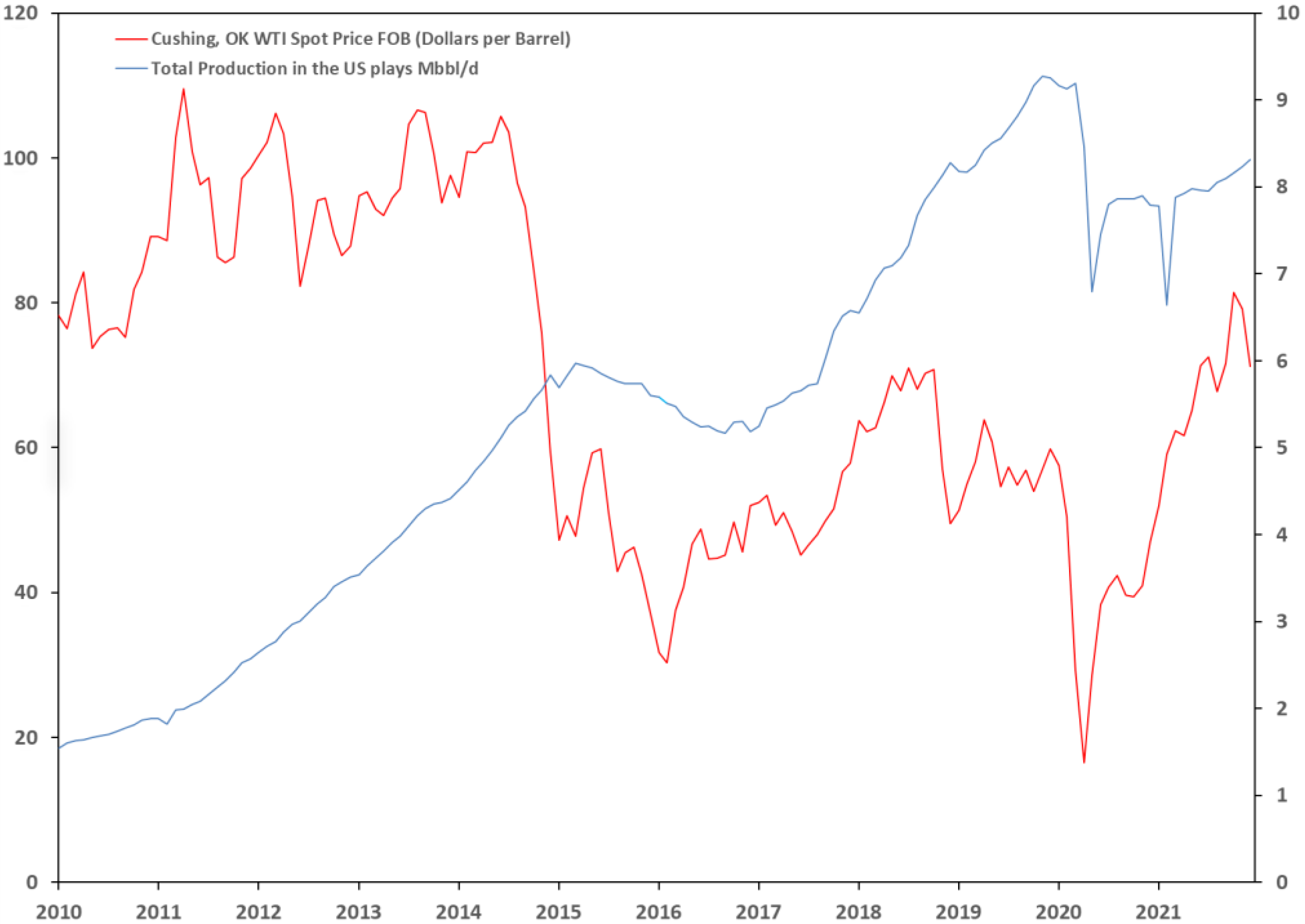
16] methodologies between 2008 and 2021. The period includes several significant incidents like the Global Financial Crisis of 2008, the price peak of 2014, the lowest of 2016 and the OPEC+ agreement, and the COVID-19 emergence and the negative prices of April 2020. We present the WTI prices and the total US production in
Figure 3.
Literature review, data, methodology, and results sections follow for further analysis.
2. Literature Review
Hubbert’s curve and its influence over oil supply have been extensively researched. It has also been used as a forecasting instrument. Brandt [
17] finds that all the historical production curves could not be fitted into a single cycle model. Past production is not well-fitted into symmetrical models while there is an asymmetry in one direction. The last implies that after the production peaks there will be a more gradual decline. Matutinovic [
18] includes factors like political agendas in oil-exporting countries and consuming behaviors in importing ones into the curve. Castro et al. [
19] research whether unconventional production could substitute the conventional one and they find that the US production data fit their model. Warrilow [
20], with his model, studies 24 countries with declining mitigation policies for resource depletion. Brecha [
21] finds that unconventional extraction rates are not enough to offset conventional production’s decrease. Sorrell et al. [
22] suggest that while data are suggesting future supply increases, there are no available data over future production decline and resource depletion. Smith [
23] proposes that scarcity should not be indicated by production peak and the rest of the indicators (unit cost, resource rent, and price) are not better either. Tilton [
24] suggests that scarcity is better indicated by prices than methodologies like that of Hubbert.
However, technological advancements alter the costs of depletion. Waisman et al. [
25] find that Peak Oil’s date is extremely dependent on short-run oil prices when the reserves are high and this leads to different price preference profiles, rent formation, and growth patterns. Low prices keep importers dependent for longer, while exporters balance this condition against long-term revenues. The sacrifice of current revenues against low long-term revenues is attractive to exporters if they hold high reserves. Importers can initiate global climate policies to escape their oil dependency and market uncertainty. Dale and Fattouh [
6] suggest that Peak Oil demand is extremely difficult to forecast due to the assumptions one has to make and that demand will continue to be strong in the future. Exporters have to diversify their economies before the complete energy transition and thus oil prices will be shaped by social costs and not by extraction costs. Okullo et al. [
26], by imposing geological constraints on Hotteling’s model find that marginal profits increase as production decreases, and hence global peak oil production will decrease since large producers will hold their production. In turn, high future prices will not increase supply.
Peak Oil has considerable effects. De Almeida and Silva [
27] suggest that mitigation policies like energy efficiency, alternative energy sources, and sustainable energy solutions will come much later than Peak Oil and the following abrupt decrease. This will cause considerable social and economic problems. Friedrichs [
28] proposes that the sociopolitical repercussions of Peak Oil are, among others, militarism, totalitarian retrenchment, and socioeconomic adaptation. Almeida and Silva [
29] propose that after the production peak, long-distance cargo transportation will become very expensive and Electric Vehicles will consist of most of the non-commercial transportation. Lutz et al. [
30] find that low elasticity and substitutability are the drivers of price explosions when supply shortages occur. To avoid such conditions, mitigation policies like energy efficiency and renewables could be implemented. Kerschner et al. [
31] worked on sectors like iron mills, fertilizers, and air transportations and found that severe damage could be caused to the whole US economy due to Peak Oil. Later, Reynolds [
32] goes even further by warning that Peak Oil could occur sooner than expected with massive inflation and economic downturns as repercussions.
However, Peak Oil is a factor with environmental aspects. Verbruggen et al. [
33] suggest that Peak Oil may be reached due to emission limitations and not by increased production. On the contrary, high hydrocarbons’ prices may finance carbon extraction investments delaying Peak Oil and extending carbon lock-in, something also later recognized by Popescu and Gheorghiu [
34]. Prideaux [
35] recognizes climate changes and Peak Oil as the main dangers to future tourism due to environmental degradation. Sioshansi et al. [
36] propose that Peak Oil will happen sooner if EVs continue to have an exponential increase. However, better Internal Combustion Vehicles’ efficiency may prevent EVs domination. Zeppini et al. [
37] find that if appropriate climate policy is not implemented then there will be a shift from oil/gas to coal exacerbating climate change. This is the reason carbon taxes, and Research and Development (R&D) subsidies for renewables should be implemented.
As a consequence, many tried to apply the model or similar models to calculate and date the Peak Oil. Holland [
38] suggests that prices can better impend scarcity than peaking and that production will peak irrespectively of the percentage of the remaining reserves. Rehrl and Friendrich [
39] apply the LOPEX model to predict oil prices and Hubbert’s curve to forecast non-OPEC supply. They suggest that prices will be high enough in 2020 while OPEC will retain a stagnating market share with 50% as the maximum. Maggio and Cacciola [
40] calculate that the Peak Oil will be between 2009 and 2021 at 29.3 to 32.1 Gbbl/y with multiple Hubbert’s curves. Gallagher [
41] detects it in 2009 with a total production of 30.4 Gbbl/y. Okullo et al. [
26] suggest that OPEC members can cause significant reserve depletion to the non-members until 2050 while decreasing the extraction rates in mature plays prolongs exhaustion date. Ebrahimi and Ghasabani [
42] with a Hubbert approach calculate that OPEC’s production will peak in 2028 at 18.85 Gbbl/y. Norouzi et al. [
43] recognize the significance of political environments in different scenarios and estimate the Peak will be reached later than 2040 in one of them while the rest suggest in the mid-2020s. Luz-Sant Ana et al. [
44] find that Norway’s production peaked in 2001 and depletion will come around 2040. Kazakhstan has not reached its peak yet while this is detected somewhere around 2023.
Meng and Bentley [
45] separate Peak Oil for conventional and unconventional production. Conventional might peak soon and thus one cannot claim that Hubbert’s curve is irrelevant due to the shale revolution. Chapman [
46] argues with those who hold Peak Oil Theory as non-valid, claiming that their data over reserves and assumptions for alternative energy production are unrealistic. These assumptions compromise energy security in the future. Energy security risks would even impact conventional producing economies as the research of Bollino and Galkin [
47] suggests.
The literature, while extended, does not give a conclusive suggestion. Thus, we are not sure if Peak Oil holds as a theory, what the maximum of productivity rates will be, and when this will happen. The literature that studies the period of the shale revolution in conjunction with Peak Oil is not sufficient enough and does to include methods similar to ours. We examine whether multiple productivity episodes of exuberance exist. Our applied methodology is innovative as, to our knowledge, it has been only used for indices and commodity prices but not production volumes.
3. Data
EIA provides productivity data for seven US regions. These are Anadarko, Appalachia, Bakken, Eagle Ford, Haynesville, Niobrara, and Permian. The data are monthly and are in bbl/rig for each region. Our data cover the period from January 2008 to December 2021. We use this kind of data to include the technological component of oil production. Hydraulic fracking and horizontal drilling were the main elements of the shale revolution. These allowed the US producers to drill only on the sweet spots and thus have the same or even higher production with fewer wells. Profoundly, this is the reasoning for selecting the production per rig as the productivity’s data.
Our research starts with the ADF test [
48] for the whole period and we find evidence that all productivity data are I(1), i.e., they are stationary at first difference (
Table 1). This is an indication that our data do not have constant specifications at each point. This is an initial indication that there might be explosiveness, i.e., producers can alter their production per rig abruptly. If prices are high then they can take advantage of it and increase their production, while when prices are low, they can almost totally cut their production.
4. Methodology
A common econometric precondition is that of stationarity. The prerequisites for the data to be stationary are that the mean, variance, and autocorrelation structures are constant over time. However, this is not the case in real life. Data through time might have trends, inconstant variances, or seasonality. Thus, this is the reason for stationarity testing. Constant mean, variance, and no trend reveal that the values are around a certain value. However, in finance there are seasons of extreme “exuberance”, i.e., asset prices increase or fall having multiple means and experiencing clustered volatility depending on the studied period. It was this phenomenon that made many econometricians develop anticipative dating algorithms for ongoing assessment. Their efforts for developing models which can detect when a time series is off its stationary processes cultivated in developing recursive procedures. These procedures detect periods of explosiveness or “bubbles”. For example, the PWY (2011) approach applies a Sup ADF or SADF test which is a succession of forward recursive right-tailed ADF tests. The test is applied in multiple research papers with good results. However, when there are multiple episodes of explosiveness, i.e., the data contain more than one “bubble”, the test partially loses its credibility. To overcome this disadvantage, the PSY (2015) approach proposes a Generalized Sup ADF or GSADF test and a repeated backward regression technique to date-stamp the periods of exuberance. The date-stamp process is again a recursive right-tailed ADF test with flexible window widths. We apply both processes to discover when producers exceed their normal production rates. If they can exceed it several times, then they can adjust their production in conjunction with other drivers and not due to geological constraints only. There is no other research conducted with these processes on production rates in our consideration.
We start with the simple ADF test proposed by Said and Dickey [
48] which has the null hypothesis of a unit root. The formula is:
Phillips et al. [
15] (or PWY (2011)) calculate repeatedly the ADF test on a forward expanding sample sequence. Then, the test value which will be compared to the critical one is the sup value of the ADF sequence. Therefore, this is written as:
where,
is the smallest sample width and 1 represents the largest window fraction or the total sample size in the recursion. If the test statistic exceeds the respective critical values, then we have “bubbles” in the time series. Phillips et al. [
16] (or PSY (2015)), propose an even more sensitive process capable of detecting multiple “bubbles”. The GSADF test is calculated by an ADF test on subsamples recursively. The subsamples are different from the previous test since they have varying endpoints. Besides the varying endpoint, the test allows the starting point
to alter within a feasible width between 0 and
. Therefore, we have:
The two procedures can detect the episodes when the respective sequences are over those of the respective critical values. The PWY (2011) and PSY (2015) can now be rewritten:
More details are provided by [
15,
16]. For our research in extraction rates/productivity, we will use the term “explosiveness” since we do not refer to capital markets. After all, productivity rates (bbl/rig) are precisely calculated and not influenced by market sentiments or actions like speculation. We are going to detect if and when productivity rates experience abrupt changes. So far, the date-stamping processes are only applied to capital and commodity markets (Fantazzini [
49], Gronwald [
50], Perifanis [
51]).
5. Results
5.1. Summary Results
Our research started with the test statistics for the full sample. We applied the SADF and GSADF tests. The critical values were obtained by 2000 replications of Monte Carlo simulations for 168 observations. The “floor” or the smallest window of the GSADF critical value was calculated by the formula proposed by the PSY 2015,
, whose result is 25. Almost all of the statistics for each region were over their 5% and 1% respective critical values and as such we have the first evidence of explosiveness in the extraction rates. Only Haynesville rejects the 5% hypothesis of no explosiveness for the SADF test. However, the GSADF reveals that there is explosiveness in our time series. We present all our results in
Table 2.
5.2. PWY (2011) Date-Stamping Process
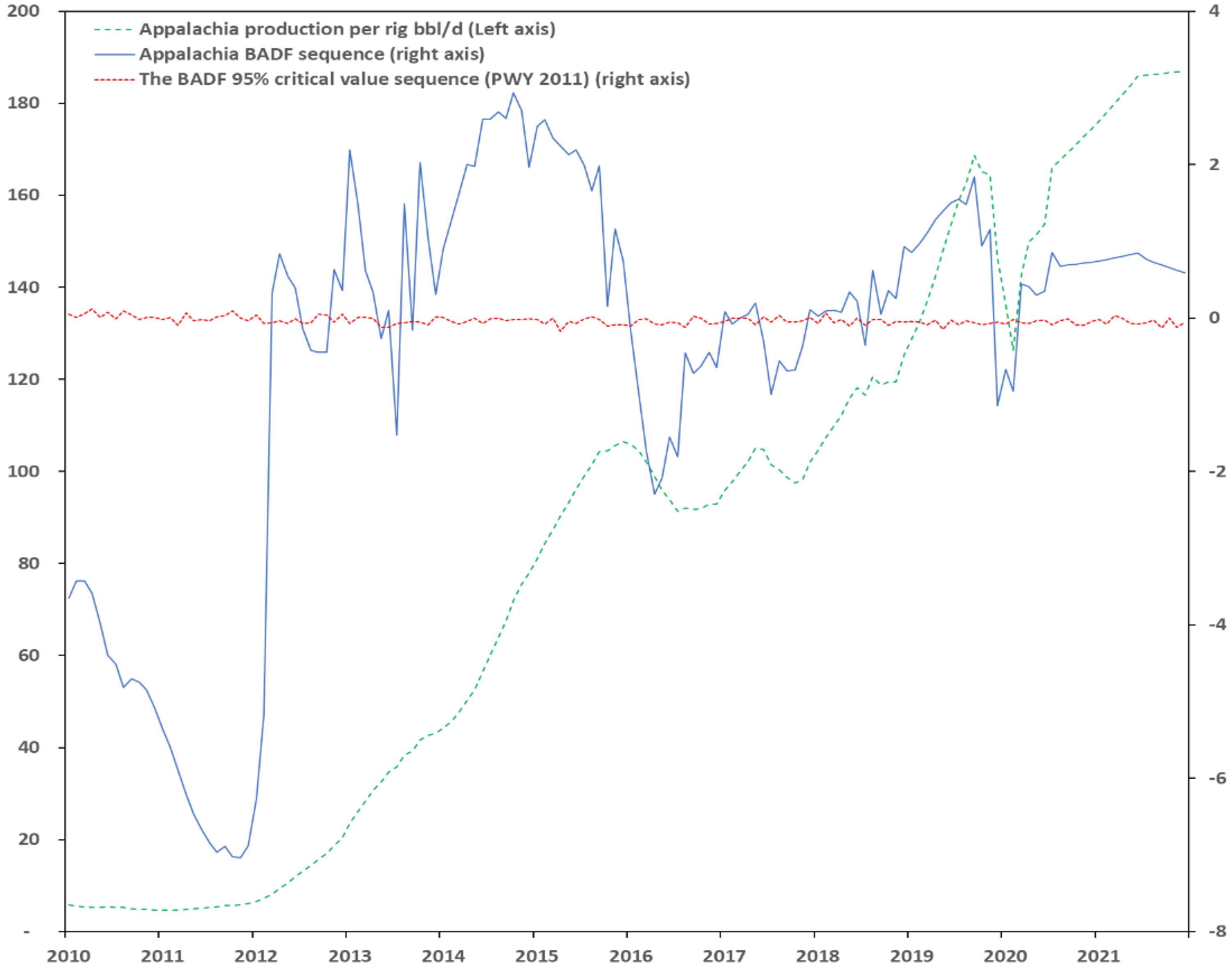
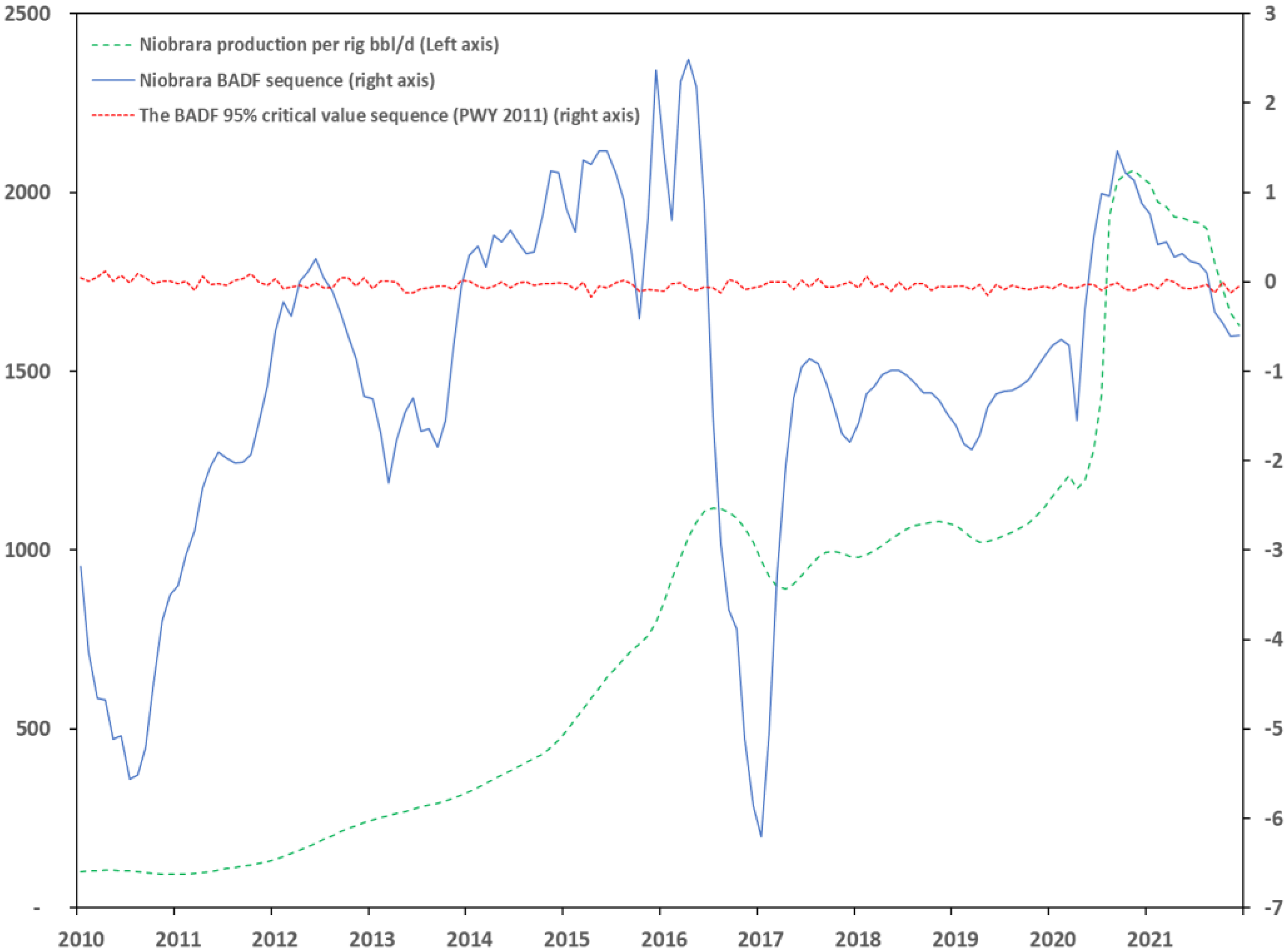
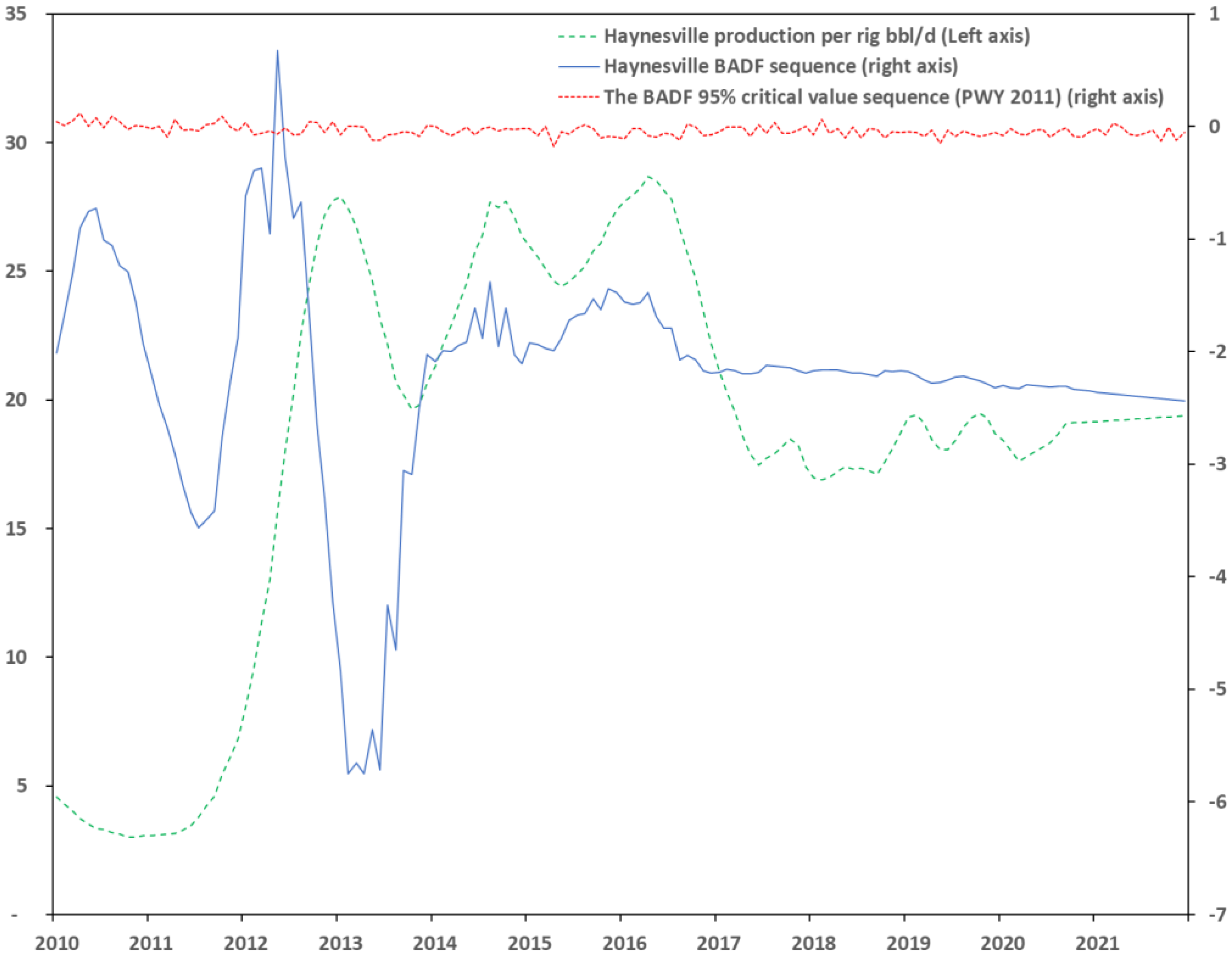
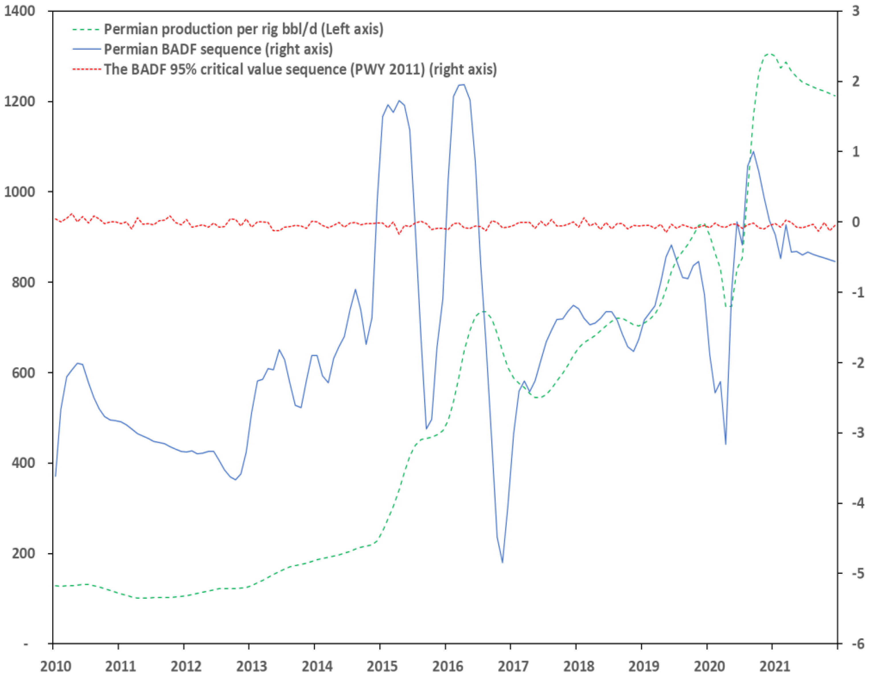
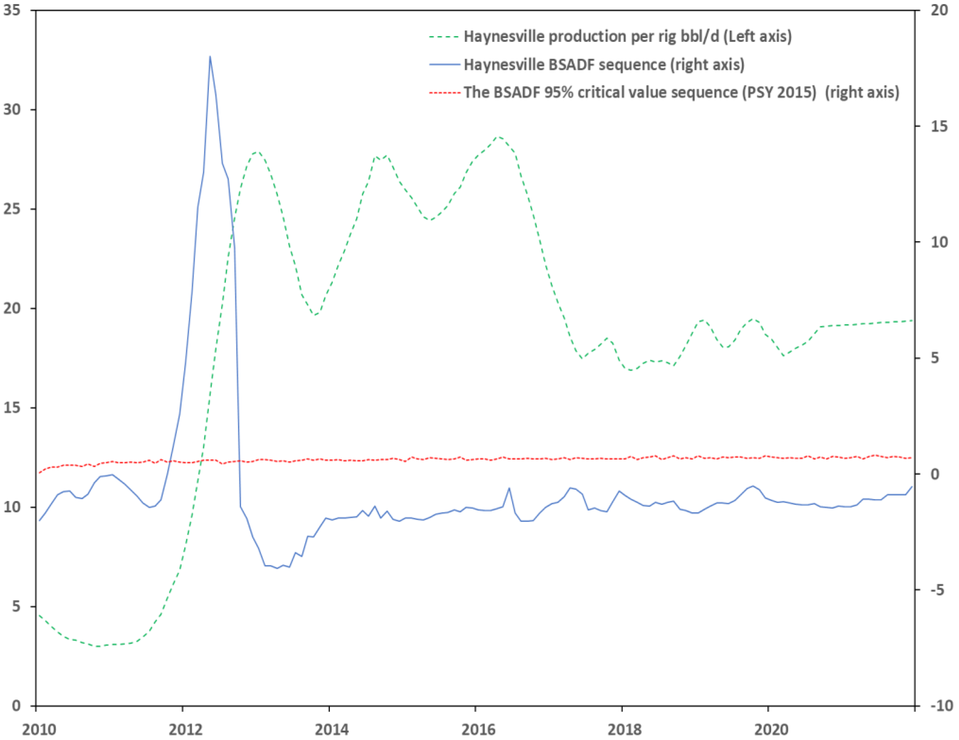
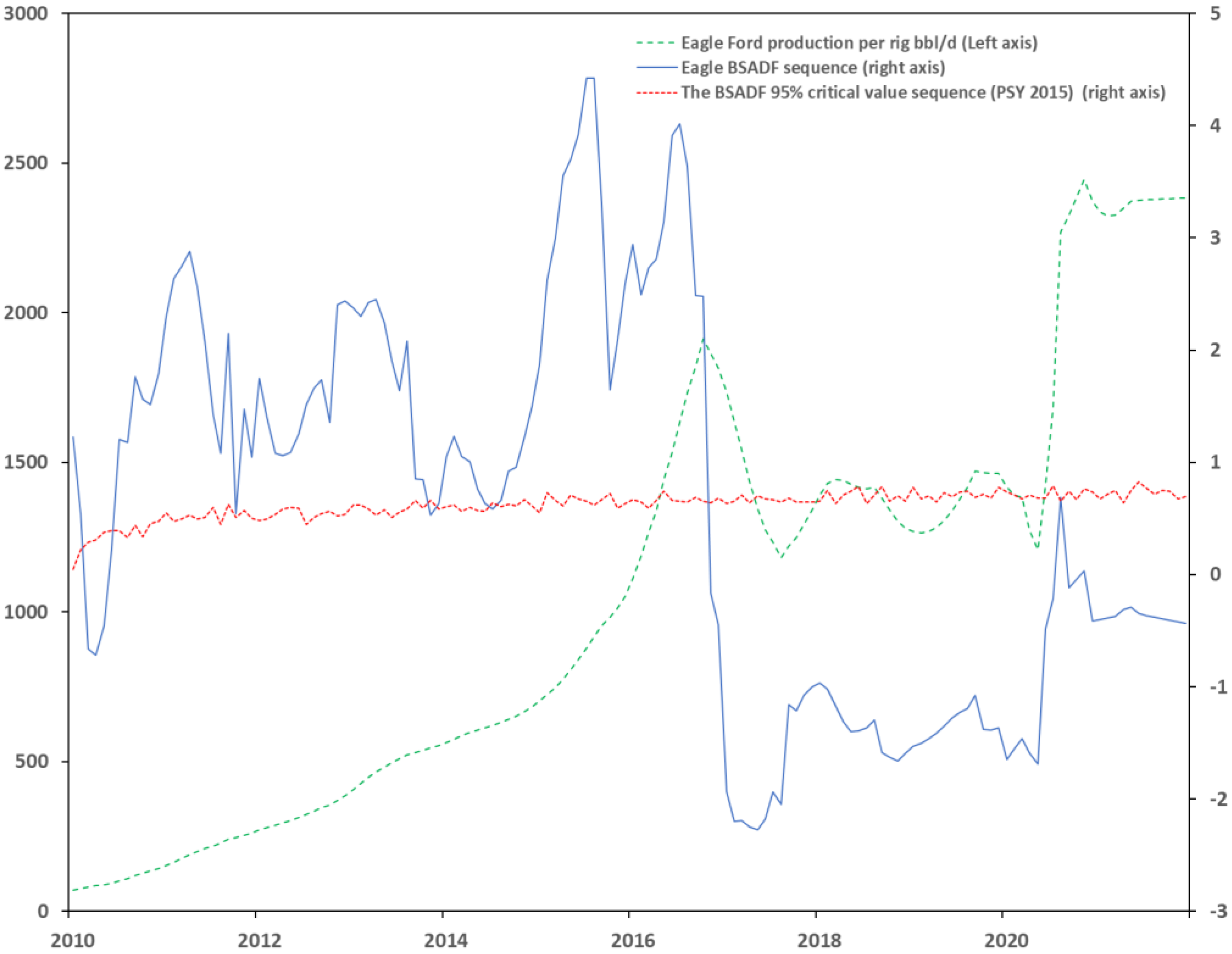
Our research continued with the date-stamping processes. We obtained the respective Backward ADF (BADF) statistic sequence and the BADF sequence of critical values for the 95% level for the PWY (2011) method. Similarly, we obtained the Backward Sup ADF sequence and the Backward Sup ADF sequence of the critical values for the 95% level for the PSY (2015) process. We graphed both sequences for each method with the respective productivity for each region. This was undertaken for comparison reasons. When a region’s statistical sequence crosses that of 95% critical value sequence upwards, then the explosive episode starts, while when it crosses it downwards, then the episode ends. As a consequence, whenever the statistical sequence is over that of the critical values then an explosive period of productivity occurs.
Starting with the PWY (2011) process, we notice that most of the regions have multiple productivity explosive episodes. The exemption is the Haynesville region whose ADF stat was close to rejecting the null hypothesis of a unit root. The region’s productivity rate increases from January 2010 to February 2013. Since then, the production rates move within a certain range between 18 and 29 bbl/d. Only when productivity exploded from 3 to 28 bbl/d an explosive episode is recognized.
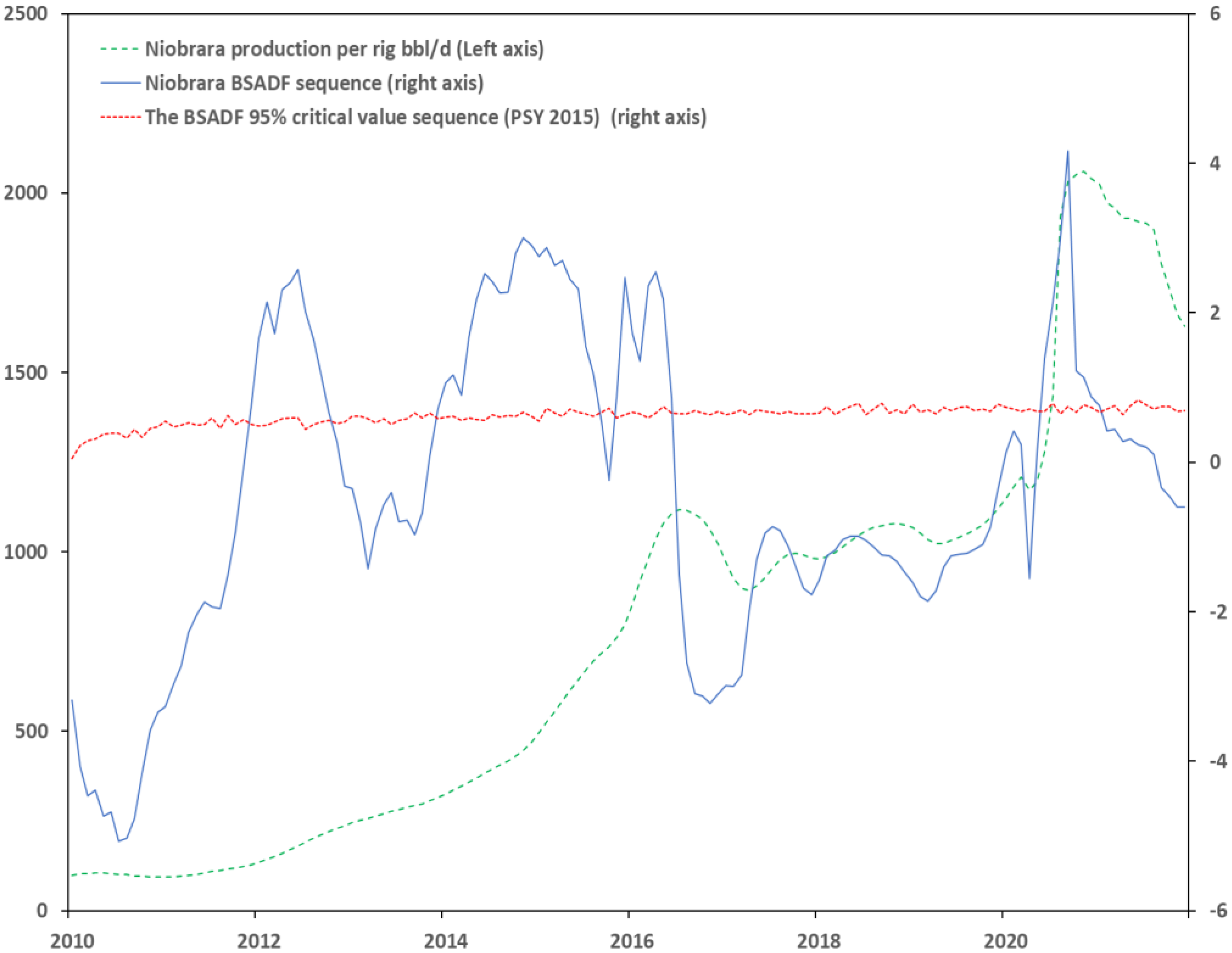
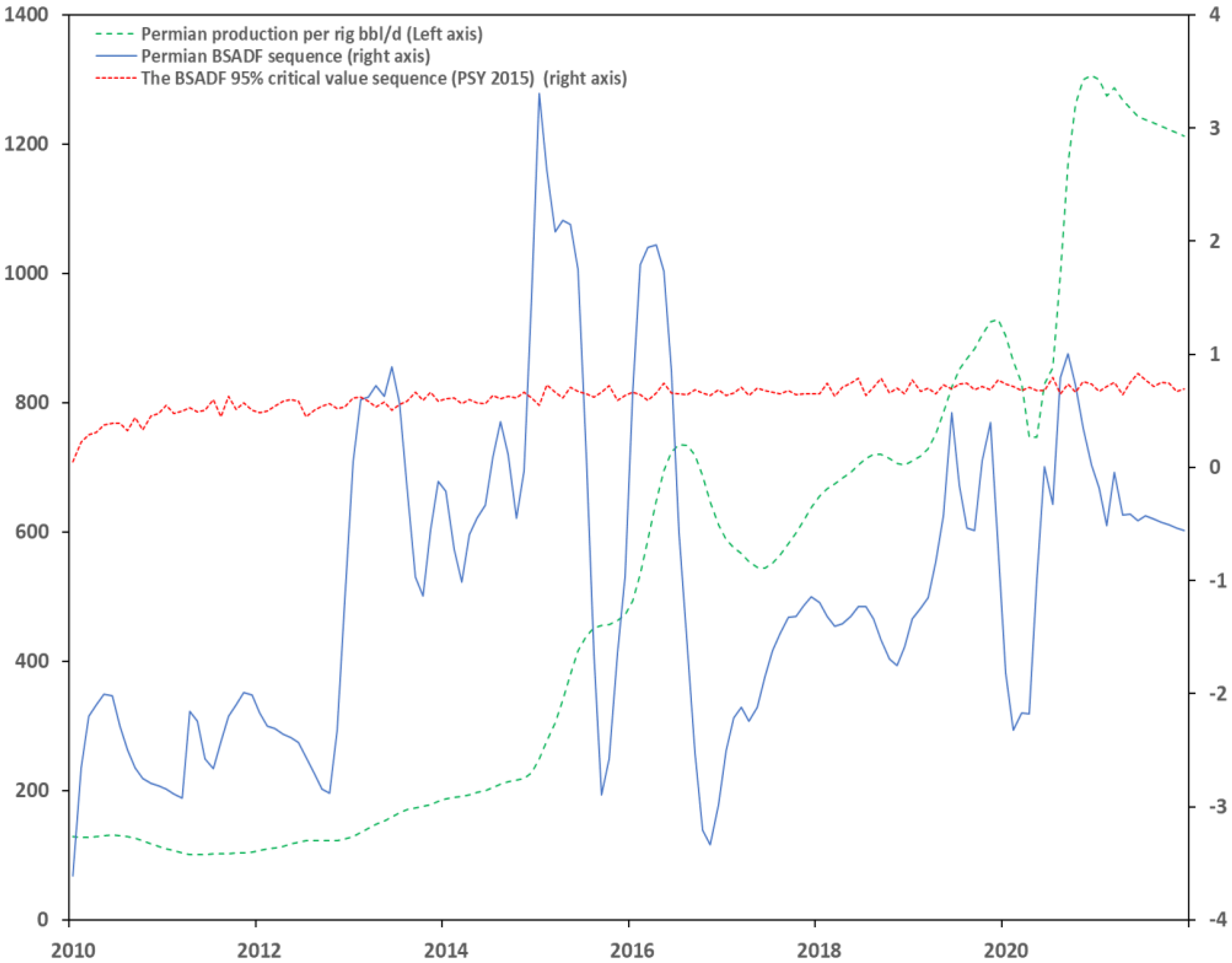
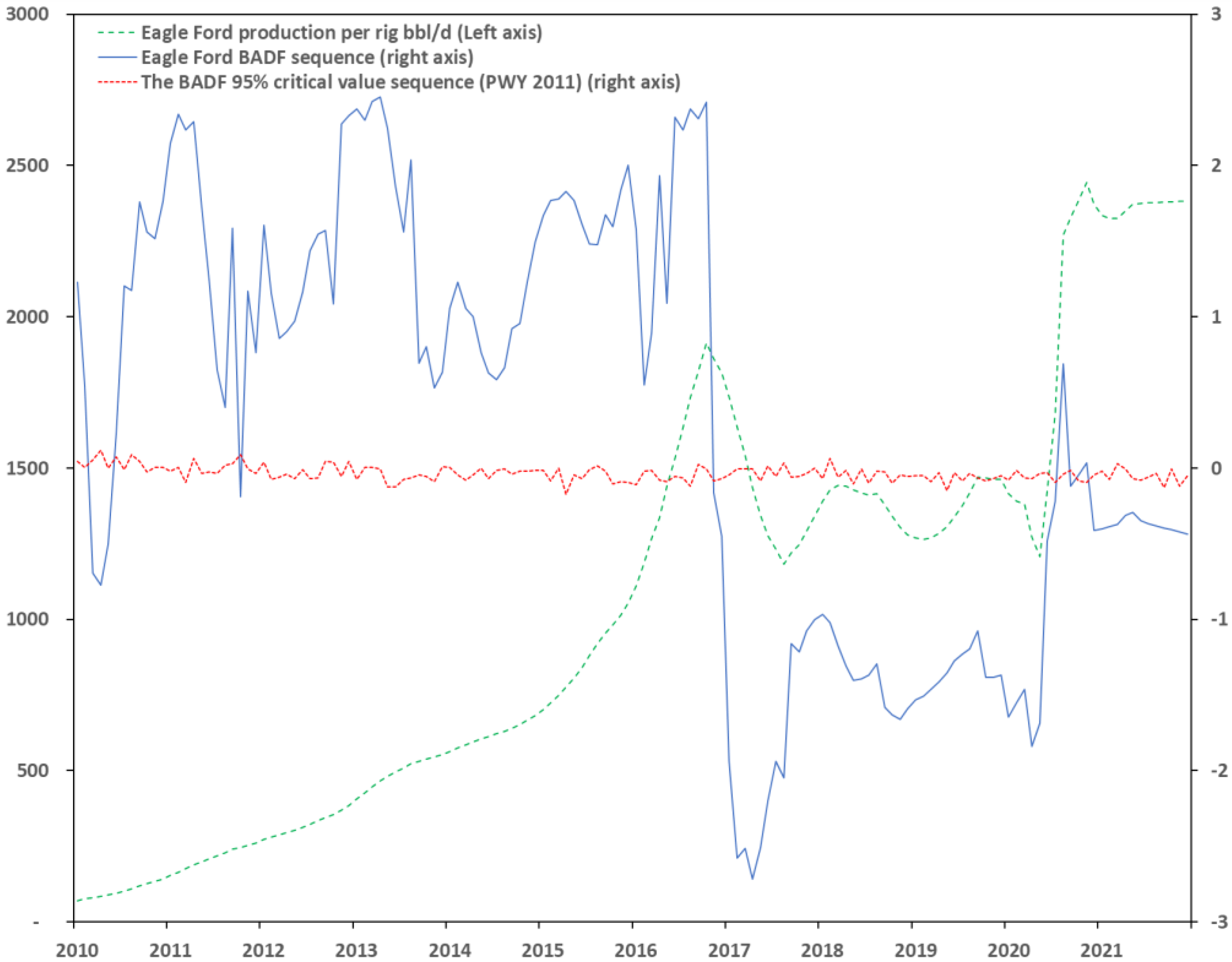
The remaining regions present multiple explosions in productivity, i.e., the producers can extract more oil per rig. The periods are mostly short. Only the Appalachia and Eagle Ford regions have periods whose duration is long, i.e., producers’ extraction rates increase constantly. However, this might be explained by the insensitiveness of the method. This is something quite interesting as producers seem to alter their extraction rates not concerning the geological conditions. Hydraulic fracturing and horizontal drilling were available across all regions. This contradiction indicates that frackers can alter their production rates depending on the market conditions. They notice price increases and they try to take advantage of them by increasing their market share. However, increased production causes oversupply when demand does not follow the increased extraction rates, and thus a glut is created. This is the reason why most of the regions experience short episodes as suppliers test how the extra volumes will influence the market.
The date-stamping process also reveals what is the most significant driver in the market, demand. After the 2008 financial crisis, oil prices increased due to the economic rebound. Demand increased and therefore suppliers in the US were ready to fix the imbalance with their increased efficiency in drilling. However, they were not alone since their increased production disrupted the market shares of traditional/conventional producers. Oil prices reached their highest level in 2014 due to the economic growth and since then decreased. From 2014 to 2016, suppliers tried to catch as much market share as they could without considering the prices or the glut. In 2016, oil prices reached their then lowest prices. OPEC+ [
52] with its Declaration of Cooperation [
53] tried to balance the market by cutting production. Conventional producers tried to drive out the shale production from the market.
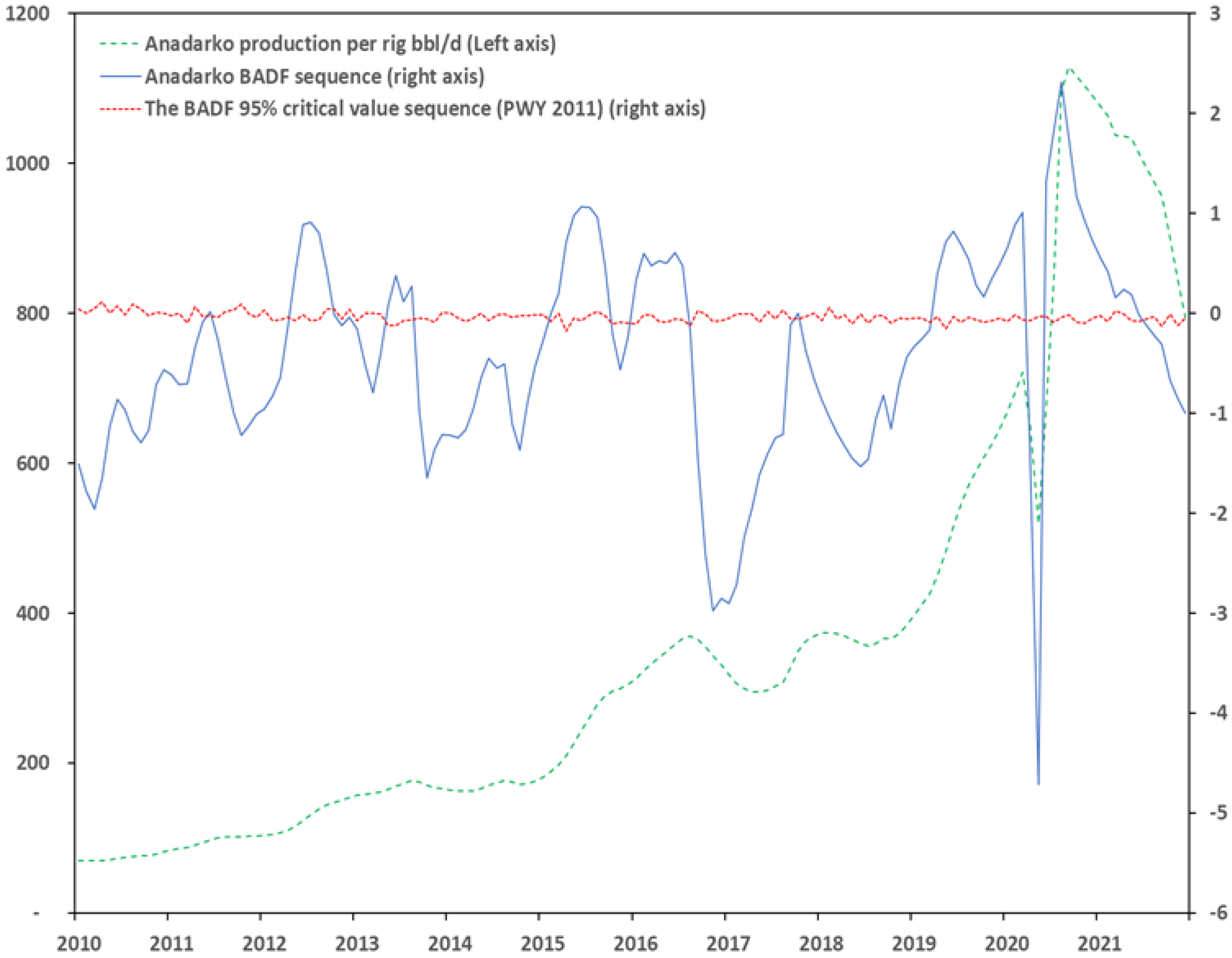
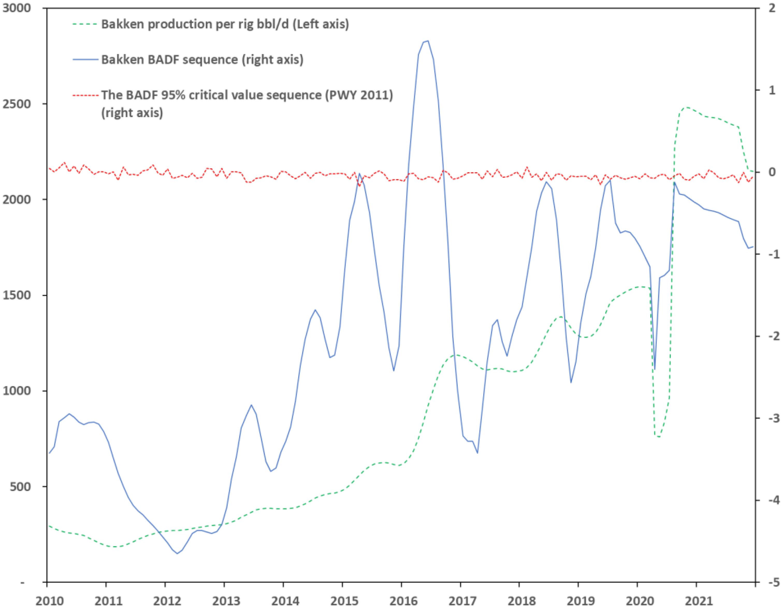
It is not a coincidence that Anadarko, Niobrara, Bakken, and Permian regions have explosive short episodes until 2016. Appalachia and Eagle Ford experience long episodes of productivity explosions until 2016. Initially, they were attempting to catch as much profit until 2014. However, from 2014 to 2016, they also had increased extraction rates to catch as much market share, something that backfired. Those extraction rates turned into a glut and increased inventories. This was a bitter experience since it took 3–4 years to have explosive episodes again. What is interesting is that there are regions with explosive episodes in April 2020 when negative prices occurred. Glut again prevailed due to the low demand caused by the COVID-19 pandemic, the increased production, the inability to export due to distribution bottlenecks, and the lack of commodity storage space. Anadarko’s explosive episode ends in March 2020, while Appalachia’s starts in March 2020, to highlight the proximity. Therefore, we agree with Christopoulos et al. [
54], Chen and Rehman [
55], and Candila et al. [
56] who recognize that the pandemic is a main disruption and volatility driver for suppliers.
On the contrary, there are many regions with short episodes starting afterward. This is justified by the increasing demand since, from mid-2020, the pandemic showed signs of retreat. Eagle Ford, Niobrara, and Permian increase their productivities to cover the ascending demand due to the economic rebound.
Finally, what is important is that producers are free from geological or operational constraints. They can alter their productivity depending on the market conditions, something which can add to the volatility of the market. Further, the multiple explosive episodes reveal that the extraction rate curve will be flattened at the top since producers will adjust their production to demand prolonging the dependency on oil. This will delay the energy transition since hydrocarbons will be available at competitive prices for a long time. We present the episodes for each region with the PWY 2011 method in
Figure 4,
Figure 5,
Figure 6,
Figure 7,
Figure 8,
Figure 9 and
Figure 10 and
Table 3. Then, we can proceed with the second date-stamping (PSY 2015) process which is more sensitive according to its introducers.
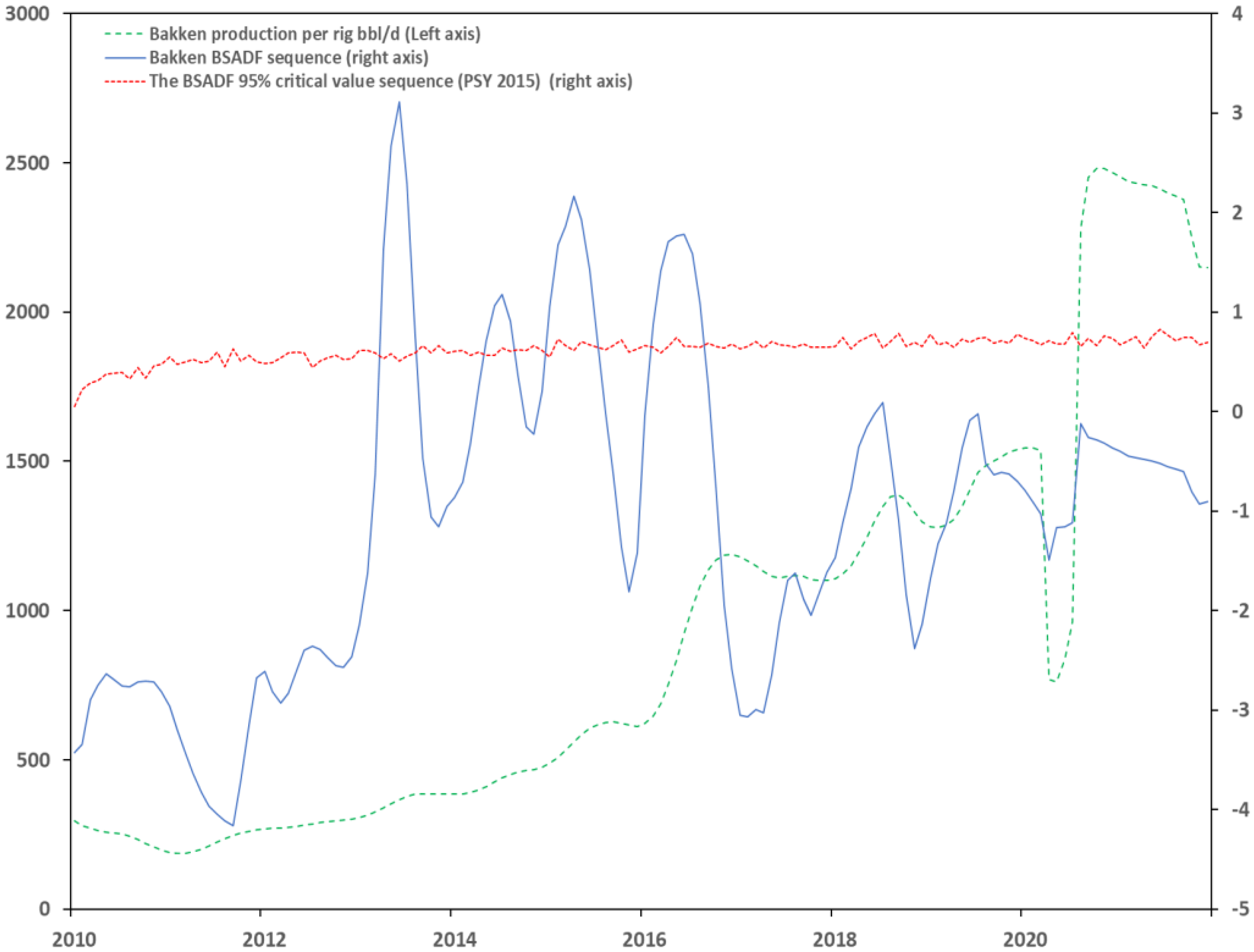
5.3. PSY (2015) Date-Stamping Process
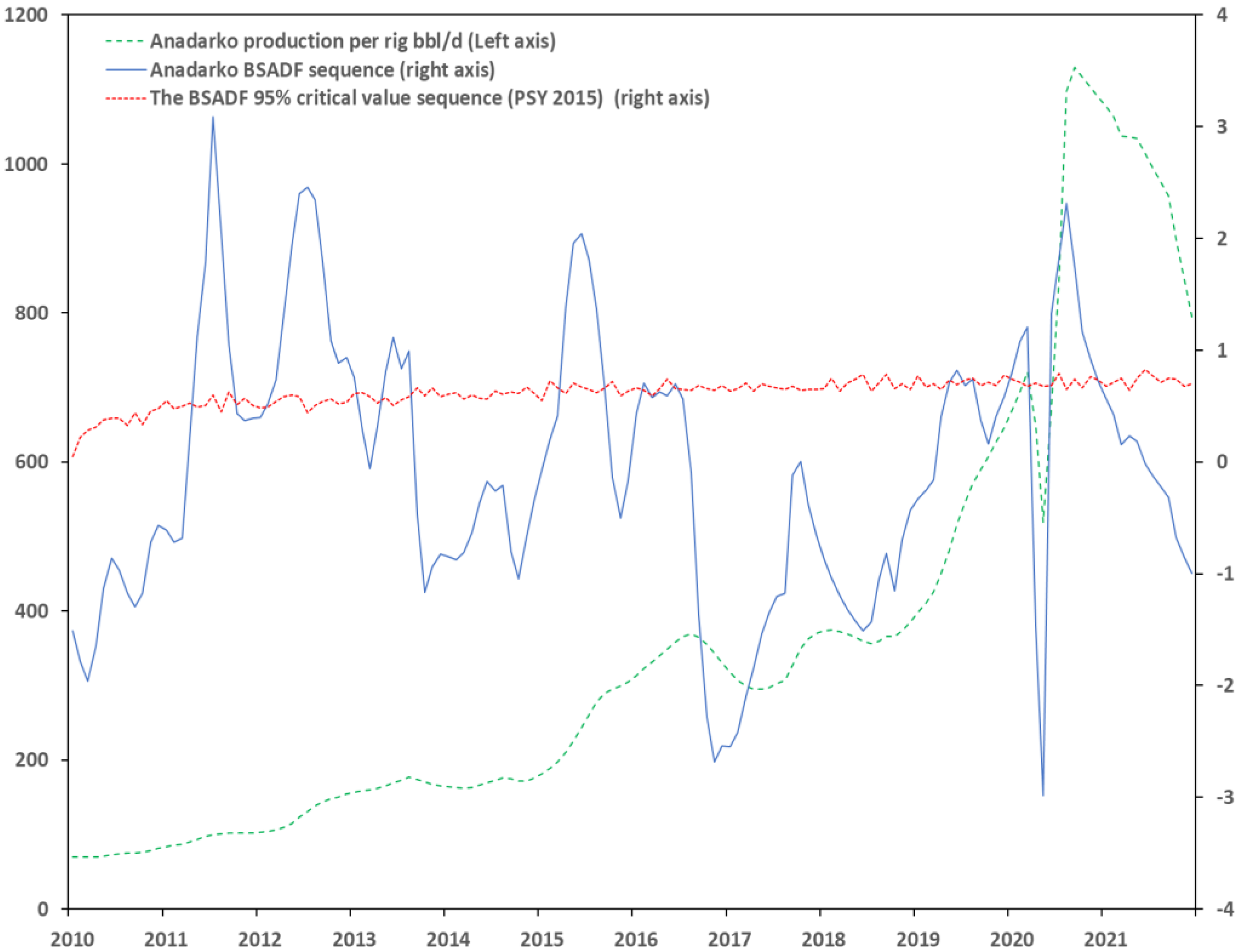
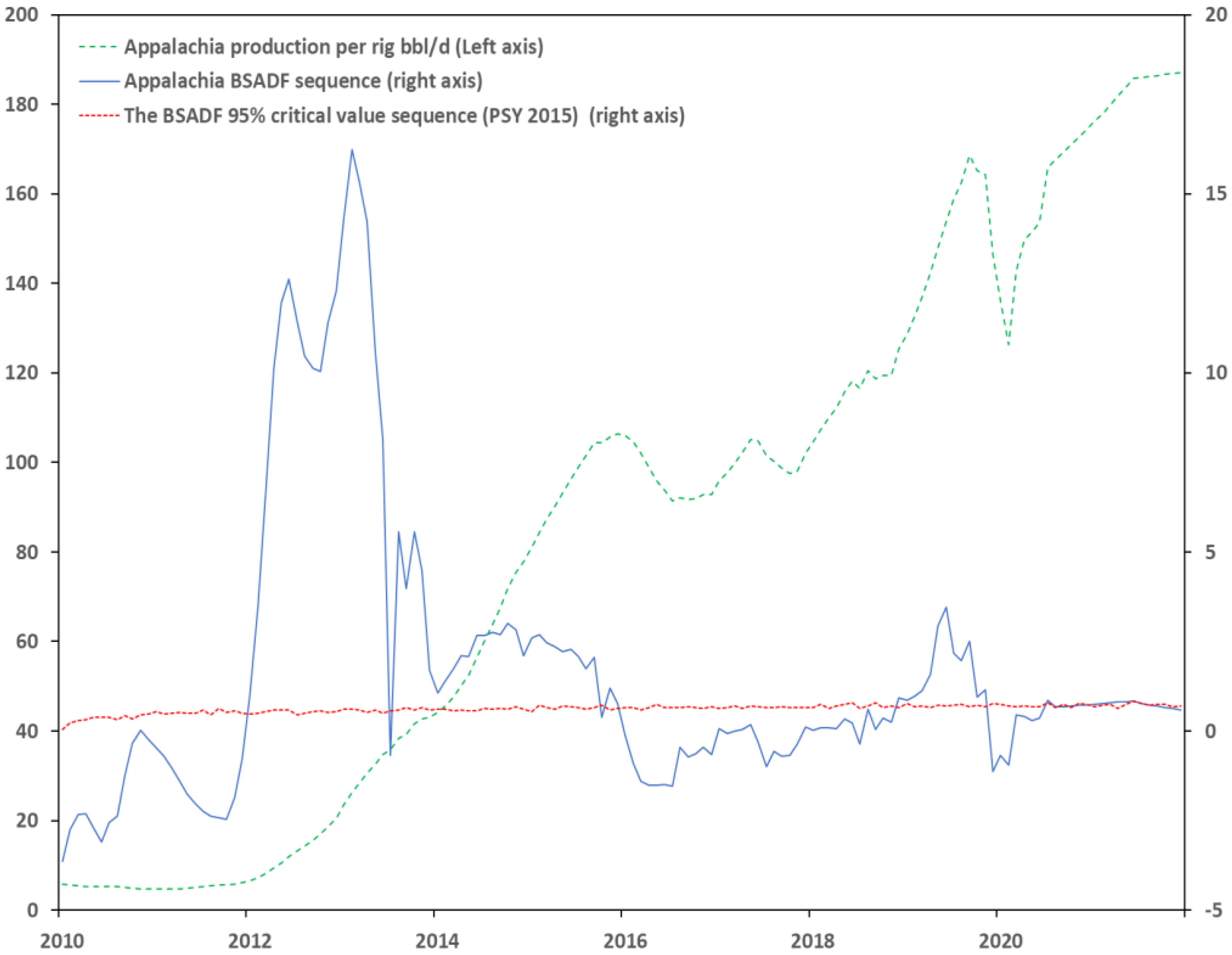
We continued with the PSY (2015) date-stamping process. For the regions Anadarko and Bakken, the method reveals more explosive episodes. On the contrary, for Appalachia, the episodes are more for the PWY (2011) method. However, the PSY (2015) reveals short-lived episodes lasting even for a month, verifying the sensitivity of the latter process. The more sensitive process reveals the short-lived character of the supply adjustments.
The last methodology reveals more episodes before 2016. It has the same justification as the previous results of PWY (2011). The US frackers can increase their efficiency and productivity rates as they favor to gain more from high prices until 2014 or retain market share from 2014 to 2016. Supply shocks are attributed mainly to demand signals. However, demand is not monitored daily, and therefore supply reacts with a lag. This kind of information asymmetry affects production decisions. One fracker may not alter his daily production but well adjust his monthly production. Production boosts or mothballs of a rig cannot be undertaken daily but a month is sufficient.
The production adjustments reveal the enjoyed freedom from geological constraints which shaped the theory of Hubbert [
1]. Now, the multiple episodes of productivity explosiveness reveal the influence of fundamentals. Since supply is not defined by geology but rather from demand and therefore prices, its peak will be flattened. It is unknown whether the US suppliers will reach the maximum extraction rates that geology can offer since demand might need to be lower than those. If demand experiences volatility, then supply will accordingly follow with multiple peaks. However, this will happen only in the short term since imbalances will be leveled out. Moreover, the energy transition will be slowed down since oil supply and therefore depletion will be prolonged. Since extraction rates will not peak, then the curve will be flattened, and then climate change will be exacerbated due to the duration of the flattened peak and the respective high emissions.
Our results agree with Matutinovic’s [
18] results that suggest that the curve will be less steep and with a fatter tail. We verify the result of Waisman et al. [
25] that low oil prices will prolong dependence. Dale’s and Fattouh’s [
6] suggestion that the Peak is too difficult to forecast due to the assumptions one has to make is confirmed. We confirm their results that oil has changed era and it is no longer scarce but abundant. Our findings agree with Okullo et al. [
26] who propose that large producers will reduce production which in turn will lower the Peak. Further, taxes on oil and therefore higher prices can enable producers to invest in new oil explorations and technologies postponing Peak Oil and extending carbon lock-in. Verbruggen and Marchoni [
33] are verified by our result for the flattening curve. Finally, Holland [
38] is confirmed, as we can also verify some of his findings (production increases are caused by demand, cost reductions due to technological efficiencies, and new exploration discoveries).
On the contrary, our results do not agree with Brandt [
17] who finds that Hubbert’s curve is the most appropriate model among the symmetric ones. However, we agree with his claim that the region whose production has already peaked will have a smoother decline rate. Our research does not verify De Castro’s et al. [
19] findings that the US unconventional production is shaped by geological conditions. Sorrell et al. [
22] are also not following our results since we find that technological evolution will maintain increased extraction rates and therefore demand will be covered. Consequently, technology will postpone depletion. Last, Smith’s [
23] claim that peaking is the best indicator for resource scarcity is not confirmed since drilling efficiency will extract enough quantities to prolong lock-in. We present the relative productivity explosion in
Figure 11,
Figure 12,
Figure 13,
Figure 14,
Figure 15,
Figure 16 and
Figure 17.
6. Conclusions
We examined whether the US regions follow Peak Oil Theory or Hubbert’s curve. If they did, then their extraction rates should experience a single explosive episode. Instead, our research confirms that almost all regions experience multiple explosive episodes, mostly short-lived. As a consequence, we can tell that our hypothesis is rejected between 2008 and 2021 and that Peak Oil cannot describe US production.
Our results suggest that suppliers can alter their production per rig depending on market fundamentals (demand and therefore prices). This is extremely important since supply is not restricted by geological constraints. However, increased productivity rates should be used with caution since supply reacts to demand signals with a lag and can turn into a glut. Even if the US suppliers’ behavior is fundamentally explained, it may cause increased volatility in the markets if they overreact to demand signals. Our results provide evidence that the US suppliers caught the economic rebound from 2008 to 2014 by producing more efficiently and that they continued by claiming extra market share from 2014 to 2016. However, this backfired in 2016 when there was an imbalance between supply and demand and the WTI prices reached their then lowest. This was again repeated in 2020 when the US suppliers continued to produce with increased extraction rates even if low demand was fully covered and there was no inventory room in conjunction with exporting bottlenecks. The repercussion was the negative prices of April 2020.
The short-living character of the episodes, especially after 2016, reveals the caution the US suppliers show to abrupt productivity changes. However, they try to take advantage of demand spikes. An example of that is the episodes in the second half of 2020. The COVID-19 pandemic and the economic slow-down eased from that point on and the producers attempted to take advantage of the demand growth. However, this was only for a few months in almost all regions. Finally, suppliers take into consideration operational issues since one is not able to increase his extraction rates constantly. It is easier to alter productivity in the short to mid-term. This secures the oil supply in the respective time horizons. Geological constraints are not an issue after the technological advancements of unconventional production.
Multiple peaks and the ability to follow the demand signals will flatten the production curve which will never reach its geological maximum. The availability of hydrocarbons will increase their attractiveness and will prolong the lock-in. This in turn may delay energy transition and exacerbate the climate crisis.


