Heat Loss Reduction Approach in Cavity Receiver Design Based on Performance Investigation of a Novel Positive Conical Scheme

Abstract

The cavity receiver’s thermal conversion performance is critical for parabolic dish and tower Concentrated Solar Power (CSP) systems. Distinct from precedent research aiming to increase the receiver’s absorption through cavity geometry optimization, the objective of this work was to investigate the thermal conversion performance of a novel, positive conical cavity receiver design, following the heat loss reduction approach with simplified pipe forming, to stress the effectiveness of this approach in cavity receiver design, and to provide data for future optimization of the proposed design. To accomplish these goals, the novel receiver and existing designs’ heat flux absorption and heat loss are compared numerically. The resulting conversion power is also experimentally validated. The concept is inspired by analysis of formulas, suggesting the novel design may realize a thermal conversion improvement of 8.6%, at 650 K, and increases with the rise in temperature. The comprehensive numerical investigation combines ray tracing of identical incoming radiation to investigate the receiver absorption and CFD methods to investigate the cavities’ heat loss at identical temperatures. The absorption acquired is unoptimized. The novel design can reduce the heat loss by as much as 91.8% when compared with a negative conical design at 650 K, resulting in a 12.3% improvement in conversion power. The experimental investigation measures the energy conversion to the working fluid in different cavities under identical incoming radiation. The novel receiver outperforms by over 5.6% in the setup. After correcting boundary conditions using experiment measurements, the experimental and numerical results are comparable. This research proves that the novel positive conical receiver has a better thermal conversion performance over 650 K; thus, the heat loss reduction approach is effective and feasible in receiver designs within this temperature range.

1. Introduction

The Concentrated Solar Power (CSP) system has a high theoretical energy density and conversion efficiency. In the CSP system, the solar thermal power is converted to the working fluid’s thermal energy by a receiver, namely, a cavity receiver in the tower or dish facility. The cavity receiver’s conversion efficiency has a critical effect on the CSP system’s performance, thus drawing the interest of many researchers.

The Concentrated Solar Power (CSP) system theoretically has high energy density and conversion efficiency. In the CSP system, the solar thermal power is converted to the working fluid’s thermal energy by a receiver, namely the cavity receiver in the tower or dish facility. The cavity receiver’s conversion efficiency has a critical effect on the CSP system’s performance, and thus draws the interests of many researchers.

The fundamental theoretical study on solar thermal conversion efficiency, which regarded the sun as a black body at 5800 K, was introduced by Petala [1]. This theory’s integration with the ideal Carnot heat engine was introduced by Jeter [2], so that it could be applied in solar thermoelectric applications. Moynihan [3] demonstrated the second law (of thermodynamics) approach to be preferable in the evaluation of the thermodynamic performance of solar thermal cavity receivers. Wright et al. [4] studied the effect of conversion stages and efficiency on the upper limit of system exergy efficiency. Researchers generally investigate the conversion efficiency using two theoretical approaches: improving the power absorption, or reducing the heat loss.

Recent solar thermal absorption research mainly uses numerical methods. Xie et al. [5] simulated the behavior of cavities in multiple geometries, receiving concentrated sunlight from a Fresnel lens, and experiments were conducted for comparison. Mao et al. [6] applied the Monte Carlo Ray-Tracing (MCRT) method to investigate the radiation flux distribution of a cylindrical cavity receiver in a parabolic dish system. Qiu et al. [7] integrated MCRT with the finite volume method to simulate the energy conversion process in a trapezoidal cavity receiver. Roux et al. [8] traced the rays in a rectangular cavity solar receiver formed by tubes and studied the efficiency of the first and second law. Pye et al. [9], traced the rays in a cavity receiver to study the heat flux distribution for the ANU SG4 solar facility. Daabo et al. [10] used the ray-tracing method to compare flux distributions in cavities of different geometries and various distances to the focal point.

Heat loss research originated from the analytical heat loss model, which divided the internal cavity receiver into a stagnant zone and a convective zone, to simplify the calculation. This was presented by Clausing [11,12]. This simplification was experimentally verified by Leibfried et al. [13]. Quere et al. [14] proposed a method using the Nusselt number at the aperture to correct the numerical results; thus, the results from different pieces of research can be cross-validated. They also suggested adding a large buffer zone outside the cavity to simulate the environment. Chan [15] built up a heat loss model with an isothermal internal cavity and adiabatic external receiver surface.

The boundary conditions found by these analytical investigations were later applied in numerical investigations of heat loss. Reddy [16,17] and Kumar [18] conducted multiple investigations on heat loss in the hemispherical cavity with different wind directions (forced convection) and inclinations, and compared the results using a 2D model with a 3D model. They found that geometry modifications could lead to less heat loss in the hemispherical cavity receiver. Xie et al. [19] numerically compared multiple tubular receivers and found the linear focus applications to have increased heat loss compared with point focus applications. Li et al. [20] numerically studied the performance of different fluids in a conical receiver and acquired the optimized temperature, flow rate, and conical angle. Issa et al. [21] compared the thermal performance in variants of conical conical receivers, finding the traditional circular design to have the maximum performance, which is also affected by flow rate. Zhang et al. [22] applied a combined numerical optics and conducted a thermal investigation of conical receivers, and the effect of conical angle, loop number, and insulation thickness on cavities’ thermal efficiency was studied.

These theoretical studies of solar thermal conversion were also verified by experimental studies. Xie et al. [19] experimentally compared the heat loss in multiple tubular receivers on a collector system with Fresnel lens. Pye et al. [23] examined the effect of multiple variables on an axisymmetric helical-coil tubular cavity receiver. The variables included solar irradiation and reflectance, flow rate, and inlet/outlet temperature. Miscellaneous experimental research also focused on the coiled pipe that formed the cavity. Chu et al. [24] studied the minimum bending diameter of $\mathsf{\Phi }$4 mm tubes. Roux et al. [8] studied the effect of different tube diameters and mass flow rates on heat conduction. In experiments, it is feasible to measure the power conversion as a whole, without the deduction of heat loss from power absorption.

In conclusion, theoretical and experimental research has shown that cavity geometries can significantly affect conversion efficiency. The investigated factors included aspect ratio, cavity geometries [19], installment angles [16], tube diameter [24], and system error [25]. Theoretical analysis results suggest that the system reaches theoretical maximum efficiency at a specific temperature [5]. As the temperature increases beyond this value, power absorption stays unchanged while heat loss increases faster than the power transfer rate; thus, the total conversion declines. Previous research suggests that the heat loss may exceed 50% [7,18] of the absorbed energy in linear and dish systems.

This paper investigates the thermal conversion performance of a novel positive conical cavity receiver design following the heat loss reduction approach with simplified pipe forming, stresses the effectiveness of this approach in cavity receiver designs, and provides data for future optimization of the cavity receiver. Numerical ray tracing and CFD methods are applied to study the receiver’s heat flux absorption and heat losses, respectively. Numerical results are experimentally validated. The heat loss reduction approach in this paper can be stated as follows: under specific conditions (radiation, work flow, temperature), the cavity receiver with reduced heat loss has an improved thermal conversion performance. To date, the author finds no such design, design approach, or integration of this design with a Fresnel lens system in the literature. The numerical and experimental results demonstrate the receiver’s thermal conversion performance and the effectiveness of the heat loss reduction design. Future improvements can be expected based on the acquired data.

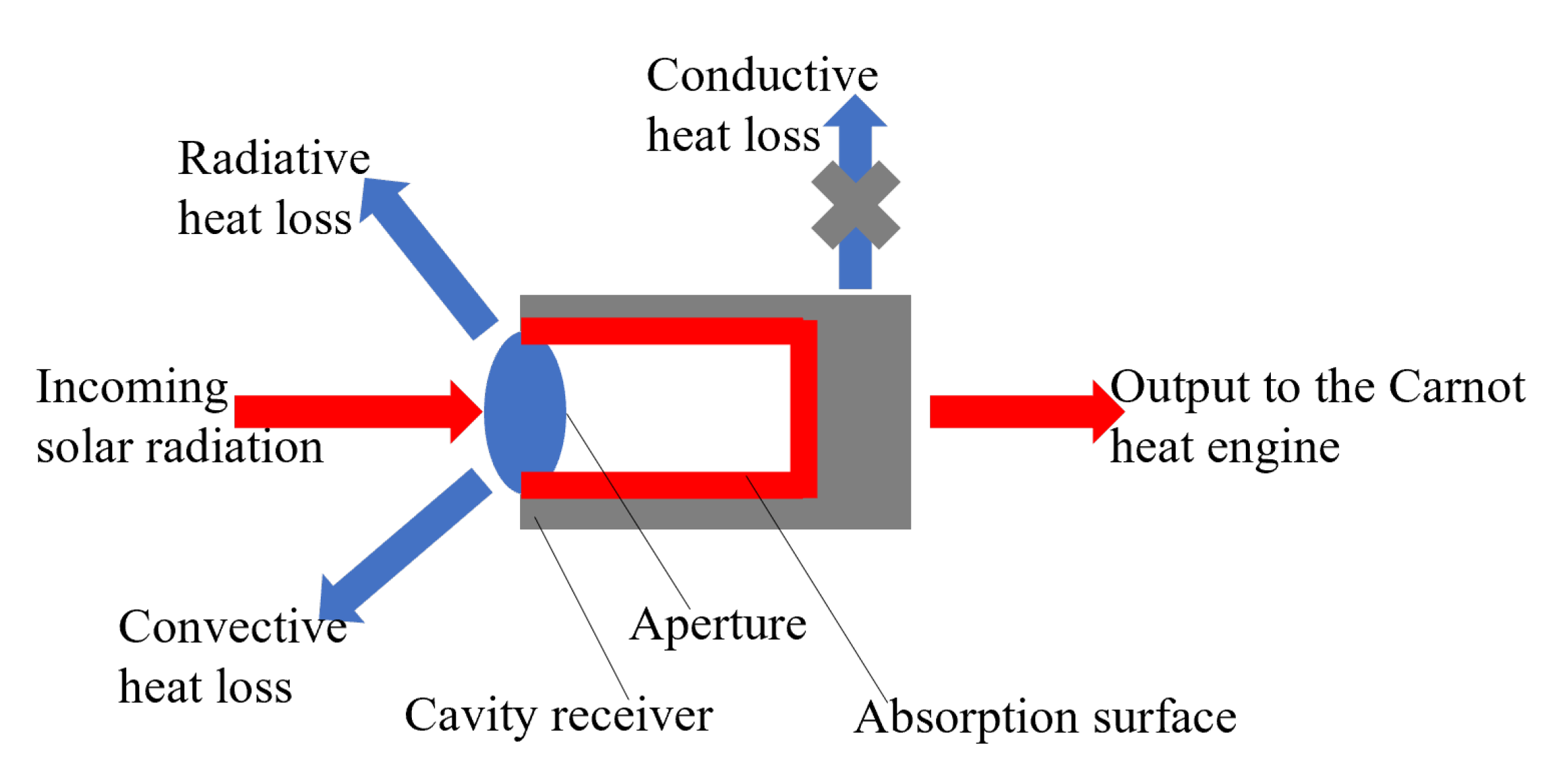
2. Heat Loss Reduction in Cavity Receiver Design

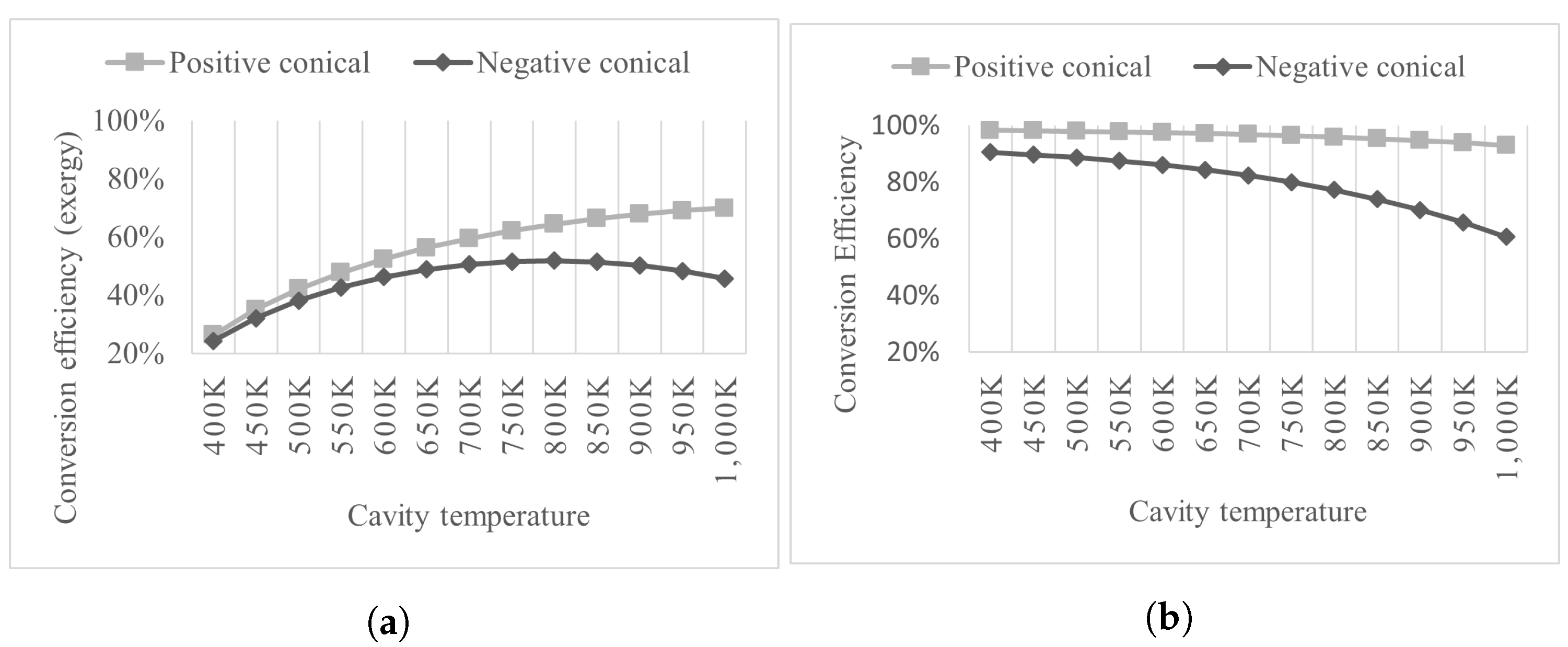
2.1. Cavity Receiver Conversion Efficiency and Discussions

The thermal conversion process is analyzed based on the classic energy flow process [3,5], demonstrated in Figure 1.

The conversion efficiency of the cavity receiver is

$${\eta }_{collector}=Q_c/Q_s$$

(1)

where $Q_c$ is the energy conversion to the working fluid. $Q_s$ is the solar radiation that reaches the receiver. The energy conversion by the fluid, $Q_c$, can be explained by the following classic equation:

$$Q_c=Q_s-Q_{rad}-Q_{cov}-Q_{cond}$$

(2)

Then, each component is considered separately. $Q_s$ Equation (2) is sometimes corrected for the effect of cavity geometry and surface absorptance [3], and becomes

$$Q_s^{\prime }={\alpha }_{ap}{Q}_s={\alpha }_W{Q}_s/\left[1-\left(1-{\alpha }_W\right)\left(1-A_h/A_W\right)\right]$$

(3)

where ${\alpha }_{ap}$ and ${\alpha }_W$ refer to the effective absorptance of the cavity and the absorber surface, respectively. $A_h$ refers to the area of the aperture. $A_W$ refers to the area of absorber surface in the cavity.

Radiative heat loss $Q_{rad}$ is expressed with the Stefan–Boltzmann Law as:

$$Q_{rad}=A_h{\epsilon }_{ap}\sigma (T^4-T_e^4)$$

(4)

where ${\epsilon }_{ap}$ refers to the effective emissivity, and ${\epsilon }_{ap}$ = $\alpha ap$ [3]. $\sigma$ refers to Boltzmann constant. $T_e$ refers to the environment temperature depending on daily temperature variation. T refers to the working fluid temperature, and this research hypothetically equals the cavity temperature.

Convective heat loss is expressed with Newton’s Law of Cooling as

$$Q_{cov}=A_h{h}_c(T-T_e)$$

(5)

where $h_c$ refers to the convective heat transfer coefficient.

Conductive heat loss is expressed with Fourier’s Law as

$$Q_{cod}=A_{c}k(T-T_e)/L$$

(6)

where $A_c$ is the contact heat transfer area, k is the thermal conductivity of the material, and L is the insulation thickness. The conductive heat loss in this research is not considered in this research, since, in this research, the absorber is actually hanging in the container through point and line contacts; thus, $A_c$ does not equal $A_W$ and is treated as zero. The research focuses on geometry factors that affect heat loss. The adopted designs have similar characteristics, which may affect heat conduction.

Finally, the energy absorbed by the working fluid can be derived as

$$\begin{array}{cc}\hfill Q_c& ={\alpha }_W\times Q_s⁄\left[1-\left(1-{\alpha }_W\right)\left(1-A_h⁄A_W\right)\right]-A_h\left[{\epsilon }_{ap}\sigma \left(T^4-T_e^4\right)+h_c\left(T-T_e\right)\right]\hfill \\ \hfill & -A_{c}k(T-T_e)/L\hfill \end{array}$$

(7)

By introducing Equations (2)–(7) into (1), the collector’s energy conversion efficiency is derived as:

$$\begin{array}{cc}\hfill {\eta }_{collector}& =Q_c⁄Q_s\hfill \\ \hfill & =\{\left({\alpha }_W{Q}_s\right)⁄\left[1-(1-{\alpha }_W)(1-A_h⁄A_W)\right]-A_h\left[{\epsilon }_{ap}\sigma \left(T^4-T_e^4\right)+h_c\left(T-T_e\right)\right]\hfill \\ \hfill & -A_{c}k(T-T_e)/L\}⁄Q_s\hfill \end{array}$$

(8)

In previous research, the exergy efficiency of a cavity receiver is usually studied. The exergy efficiency of the cavity receiver is the ratio of the exergy output to the ideal Carnot heat engine ($E_c$) to the receiver’s exergy conversion ($E_s$). It follows Equation (9):

$${\eta }_e=E_c/E_s=\left(Q_c\times {\mathsf{\Psi }}_c\right)/\left(Q_s\times {\mathsf{\Psi }}_s\right)$$

(9)

In Equation (9), $T_s$ refers to the typical temperature of the sun (at 5762 K). The Carnot heat engine and black body absorption efficiency follow the following equations:

$${\mathsf{\Psi }}_c=1-T_e/T$$

(10)

$${\mathsf{\Psi }}_s=1-4\times \left(T_e/T_s\right)/3+{\left(T_e/T_s\right)}^4/3$$

(11)

Then, the exergy efficiency of the cavity receiver in Equation (9) becomes:

$$\begin{array}{cc}\hfill {\eta }_e& =\left(Q_c\times {\mathsf{\Psi }}_c\right)⁄\left(Q_s\times {\mathsf{\Psi }}_s\right)\hfill \\ \hfill & =\{\left({\alpha }_W{Q}_s\right)⁄\left[1-(1-{\alpha }_W)(1-A_h⁄A_W)\right]-A_h\left[{\epsilon }_{ap}\sigma \left(T^4-T_e^4\right)+h_c\left(T-T_e\right)\right]\hfill \\ \hfill & -A_{c}k(T-T_e)/L\}\times \left(1-T_e⁄T\right)\hfill \\ \hfill & ⁄\left[Q_s\times (1-4\times \left(T_e/T_s\right)/3+{\left(T_e/T_s\right)}^4/3)\right]\hfill \end{array}$$

(12)

In this research, $Q_s$, ${\alpha }_W$, ${\epsilon }_{ap}$ (=${\alpha }_{ap}$), and $\sigma$ have pre-defined values or can be calculated. Let $Q_s$ = 1000 W, ${\alpha }_W$ = 0.85. $T_e$ reaches the working environment. Thus, under the theoretical assumption of contact area $A_c$ is zero, only $A_h$, $A_W$, T, and $h_c$ can affect these efficiencies.

From Equation (7), it can preliminarily be concluded that (1) the decrease in the aperture area $A_h$ can reduce reflective, radiative, and convective heat loss; (2) it is preferable for the absorption surface area $A_W$ to be far larger than $A_h$; (3) a reduction in convective heat transfer coefficient $h_c$ can reduce convective heat loss. At higher working temperatures, in cavity receiver designs, heat loss reduction can be realized following relatively simple rules. This may be preferable to helical pipe geometry optimization, which mainly improves absorption.

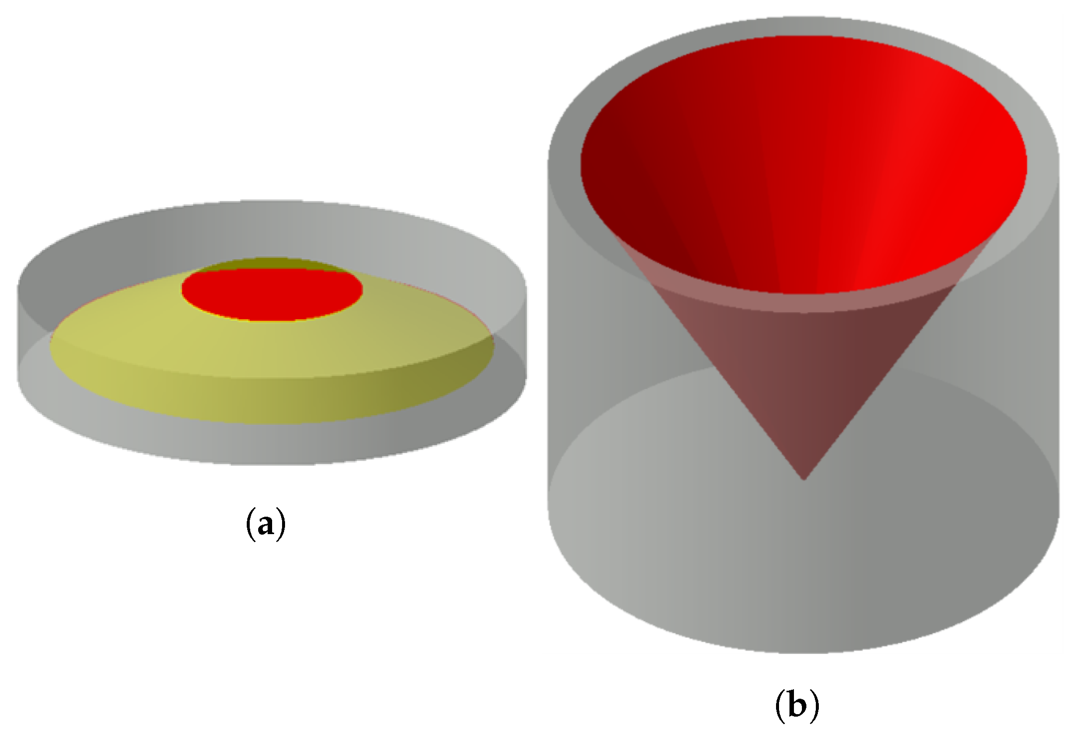
2.2. Novel Positive Conical Cavity Receiver Scheme

2.2.1. Receiver Scheme

To demonstrate the effectiveness of the heat loss design reduction approach, a novel receiver scheme is proposed. To limit the effect of absorption optimization, a planar allocation of the helical pipe is adapted. The following strategies are also considered: (1) use the point-focus (of light) to realize a high concentration ratio and conversion efficiency; (2) decrease the dimensions of the aperture to benefit installment and maintenance; (3) the cavity receiver can be applied in a new Fresnel lens collector module to reduce the sunlight blocked by structure.

The schematic cavity is a frustum of a positive cone, as shown in Figure 2, with a new collector module concept with a Fresnel lens.

Concentrated radiation reaches the helical pipe absorber surface at the base through the aperture at the apex. The aperture with a small diameter and lateral face with high reflectivity reduce convective heat loss and light emissivity. The absorber is hanging in the cavity with no contact with the insulation layers to reduce heat conduction. A small height is predefined, as it is expected that part of the convective energy can be utilized to heat the outer rings of the helical pipe.

This scheme is inspired by the existing design by the Australian Solar Thermal Research Initiative (ASTRI) [9]. Their comparison is shown in Figure 3. The novel design has simplified the geometry forming the pipe and utilizes convective heat by reducing the cavity height.

This receiver can be used in a parabolic CSP facility. In the future, this application is expected to be used in a solar thermoelectric facility, shown in Figure 4. The working fluid (air) is heated in the collector modules utilizing a Fresnel lens. These modules are serially connected to the output of high-temperature working fluid to operate the power generator.

2.2.2. Analytical Investigations

The new cavity with a traditional negative conical cavity is used for comparison. Their geometries can be seen in Figure 5.

Their dimensions are listed in

Table 1. Cavity dimensions for analytical investigation.

	${\mathit{A}}_{\mathit{h}}$	${\mathit{A}}_{\mathit{W}}$	Height
Novel positive conical receiver	1590 mm${}^2$	18,626 mm${}^2$	15 mm
	($\mathsf{\Phi }$45 mm)	($\mathsf{\Phi }$154 mm)
Negative conical receiver	9503 mm${}^2$	19,006 mm${}^2$	95.3 mm
	($\mathsf{\Phi }$110 mm)	(Apex angle @ 60°)

.

For the novel positive conical cavity and the traditional negative conical cavity, the thermal power conversion efficiencies are 97.20% and 84.35% at 650 K, respectively, while the environment temperature is 300 K. The exergy efficiencies are 56.24% and 48.81%, respectively.

The cavity exergy conversion efficiency from Equation (12) and power conversion efficiency (energy) from Equation (8) at 400 K to 1000 K, and an environment temperature of 300 K, is shown in Figure 6. The new positive conical cavity has a superior theoretical thermal performance.

At a specific working temperature, under identical incoming radiation and working fluid flow rates, a higher cavity energy efficiency will lead to higher exergy efficiency; thus, only the cavity energy efficiency is investigated in this paper.

3. Numerical Investigations

The numerical investigation aimed to numerically compare the novel cavity receiver’s thermal conversion performance with existing designs. This included two steps:

• The solar thermal absorption was calculated using the ray-tracing method and compared under an identical incoming flux.
• The heat losses from the cavity were investigated using the CFD method and compared at identical temperature levels.

Thermal conversion power is calculated from the results of the two steps presented above. Reasonable working conditions and assumptions are applied in the numerical investigation.

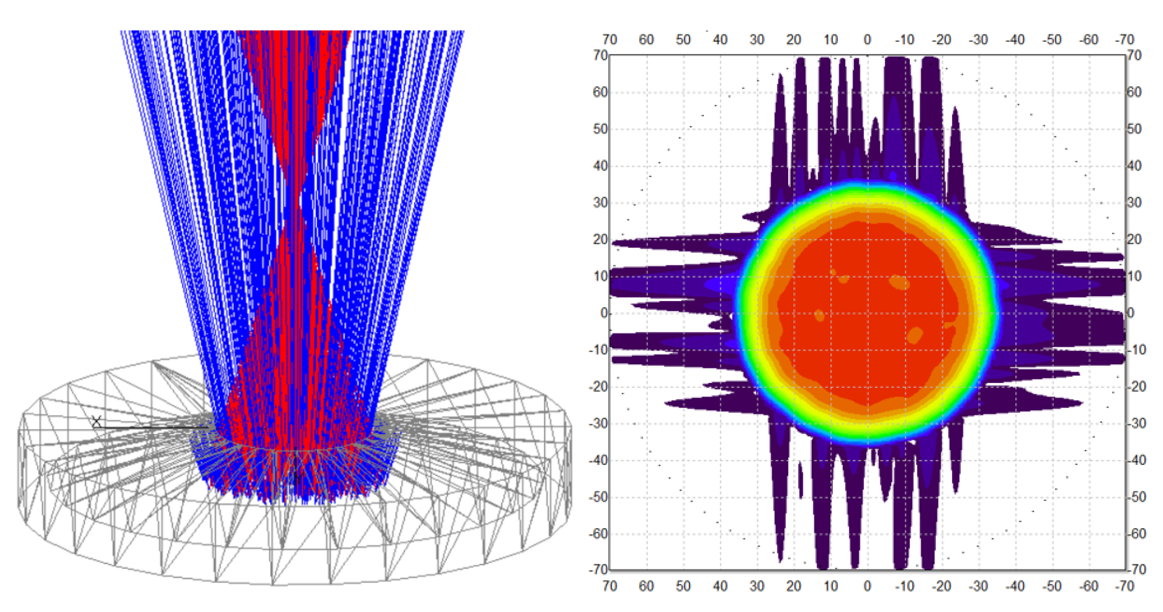
3.1. Solar Thermal Absorption Analysis

In the heat loss reduction design approach, the absorption power is preliminarily required, because (1) it is necessary to obtain the thermal conversion and (2) it needs to be reasonably high to heat the cavity to the specific temperature required for comparison. The ray-tracing method was applied to investigate the thermal power absorbed on the absorber surface under an identical incoming flux.

The ray-tracing numerical method utilized the following 3D models:

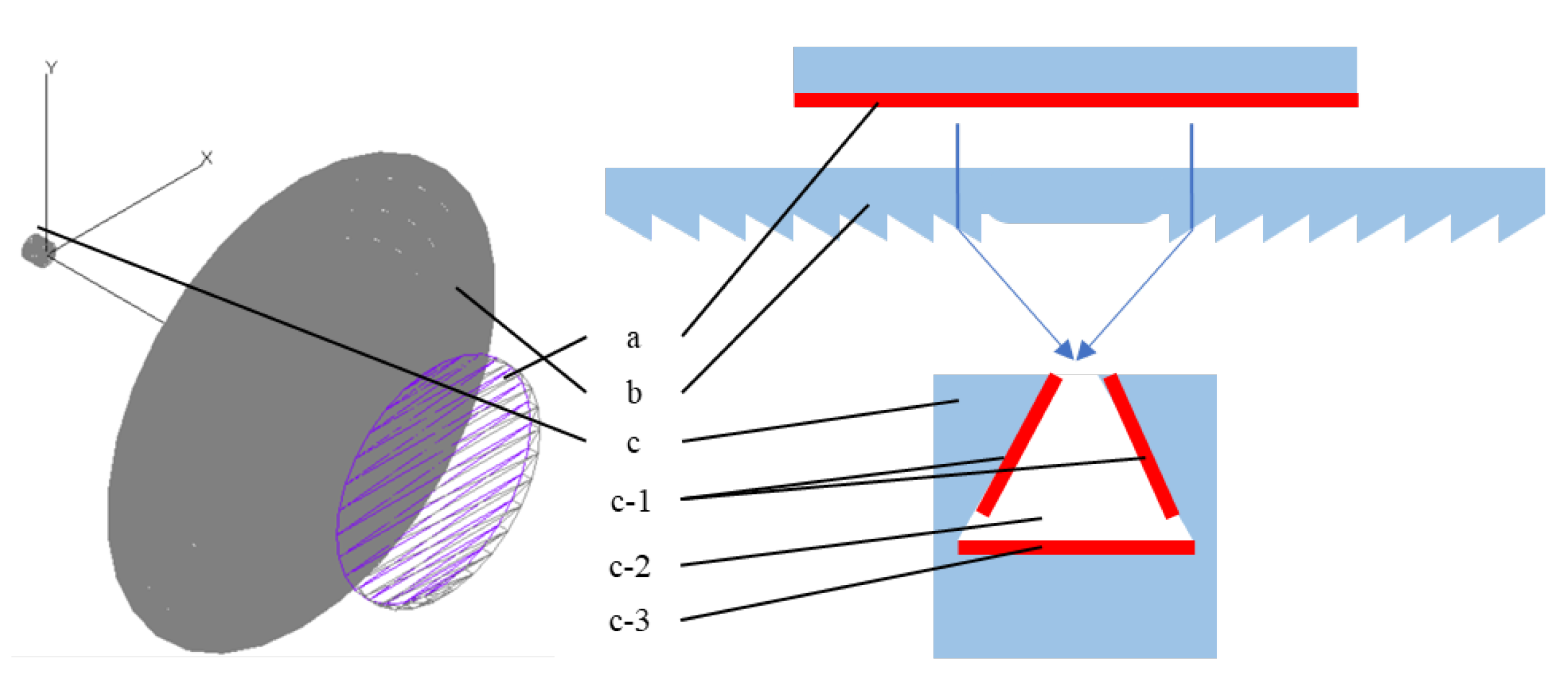
• Light source: Circular, diameter 400 mm, heat flux 1000 W, and a total of 2000 rays traced.
• The Fresnel lens: Circular, diameter 500 mm, ring width at 0.5 mm, height 5 mm, and focal length 630 mm.
• The cavity receiver model: Simplified into a one-piece 3D model. The novel receiver’s case is shown in Figure 7, whose internal lateral cavity surface’s reflectivity is 80%. The base diameter is 154 mm.

The distances between the lens and the aperture were adjusted at a minimum of 0.5 mm intervals, ensuring the maximum absorption of traced rays. The factors affecting the receiver’s thermal absorption are investigated in the following order:

• Dimension factors, including the frustum (cavity) height and the aperture diameter. The heights range from 15 mm to 45 mm. The aperture diameters range from 30 mm to 60 mm. Only the proposed positive conical design is studied. The results are listed and discussed in Section 5.1.1.
• Surface absorptance. The base surface absorptance range from 70% to 95% is investigated. Only the proposed positive conical design is studied. Numerical results for different absorptances are listed and discussed in Section 5.1.2.
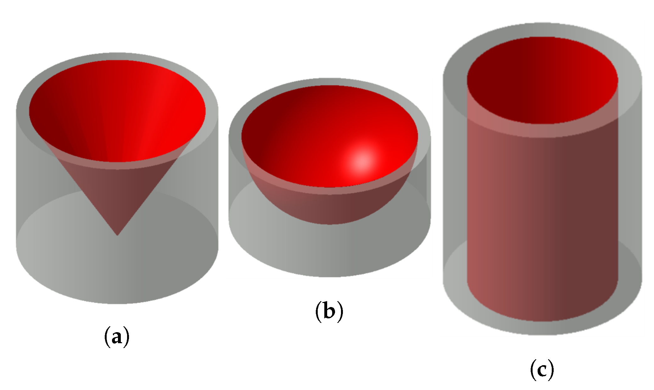
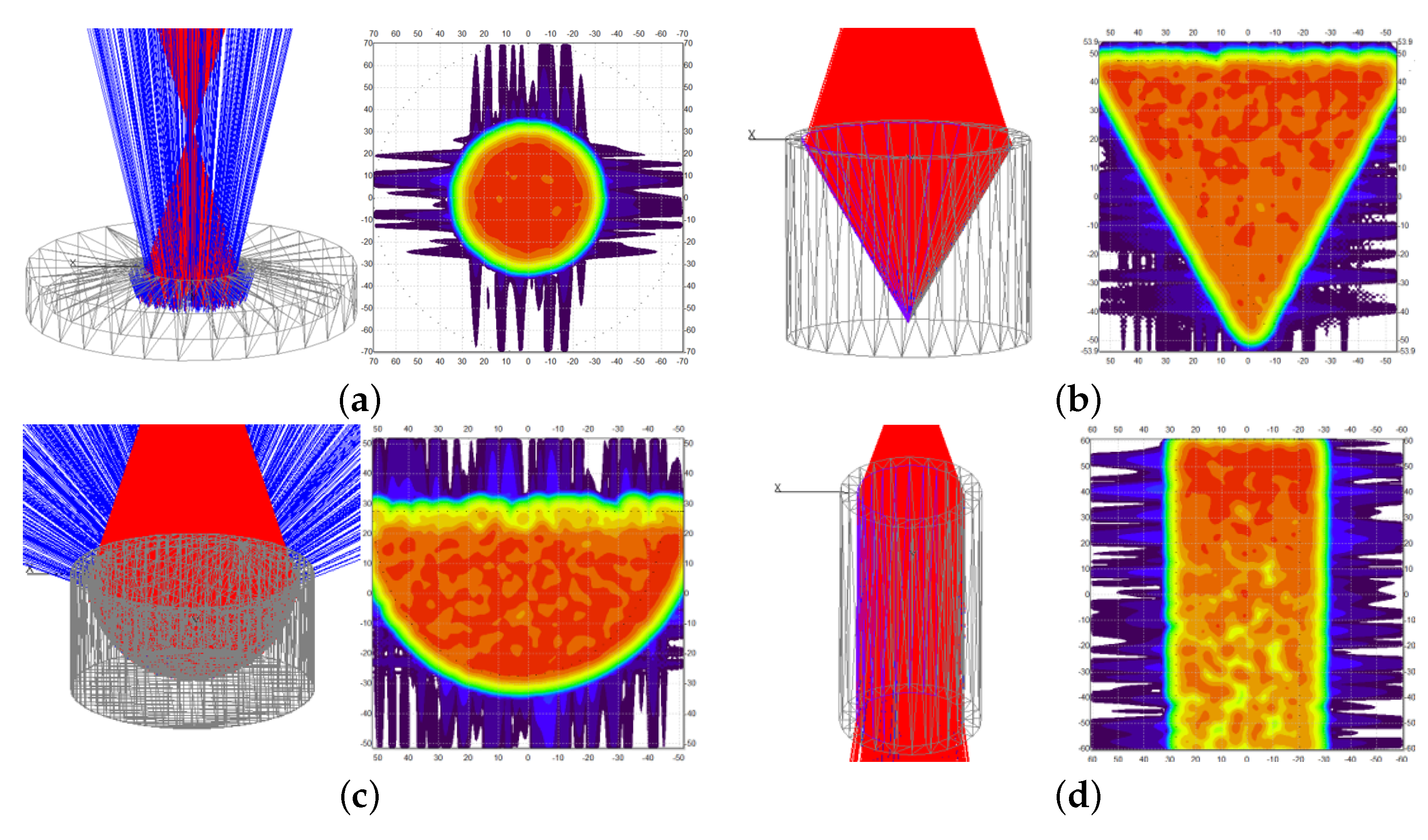
• Geometries. The proposed positive conical design is compared with the existing design of different geometries, which are negative conical, hemispherical, and cylindrical, respectively. These cavities share a comparable absorber area with the positive conical receiver. The 3D details and absorption results of the cavities are listed and discussed in Section 5.1.3.

Absorption optimization is not the focus of this research. The ray-tracing results are applied to obtain the cavities’ thermal conversion power under specific conditions (incoming radiation, environment temperature). The absorption analysis also provides data for future improvements in the proposed design.

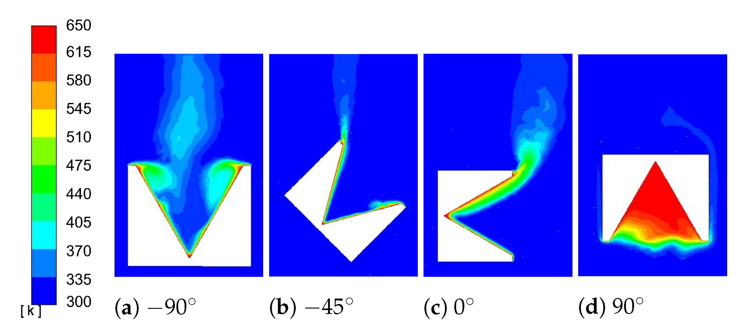
3.2. Heat Loss Analysis

The investigation utilizes ANSYS Fluent software.

The reduction in heat loss presented by the proposed cavity receiver is the focus of this research. The heat loss values are also essential in the calculation of instant thermal conversion power. The CFD method is applied to investigate the radiative and convective heat loss power from the internal faces of different cavities at specific environment and cavity temperatures.

To simplify the analysis, the following assumptions are reasonably adapted:

• The heat losses are compared at identical cavity and environment temperatures.
• The acquired heat loss is an instant value in the conversion process under the working conditions shown above.
• The cavities’ external and internal faces are isothermal.
• The conductive heat loss from the pipe to the receiver is neglected, as discussed in Section 2.1.
• The conductive heat loss from the receiver to the supportive structure is neglected, as discussed in Section 2.1.
• Only the air is modeled with volume.
• An adequate buffer zone is left between the domain’s boundary and the cavity, so that the domain’s boundary is regarded as ambient air [15]
• The air is assumed to be incompressible to simulate the air flow caused by heating.
• The thermal process is assumed to be steady-state.

The numerical CFD investigation of heat losses is processed in the following order:

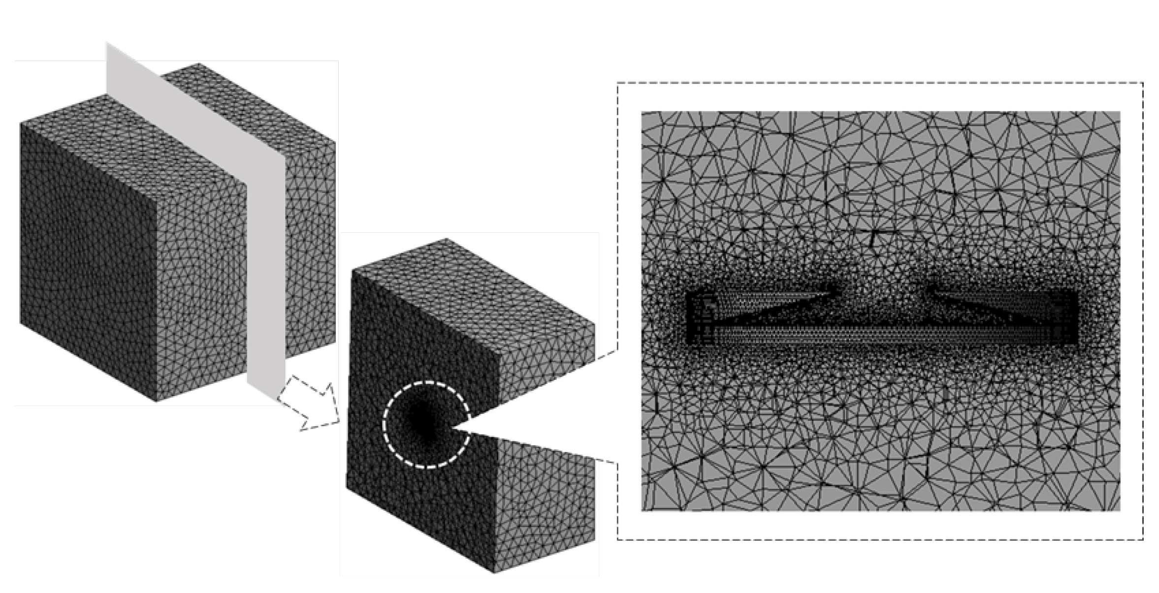
• Geometry. The external geometry of the 3D air model is cubic with an edge length of 3000 mm. The solid body of the cavity is excluded from the numerical investigation into radiative and convective heat losses.
• Meshing. There are at least 20 elements along a single edge. The cavity surface is intensively meshed with elements smaller than 1 mm. The tetrahedron patch conforming method is designated for the entire body. The final mesh result is shown in Figure 8 with a quality over 0.8.
• CFD models. The energy equation is activated according to 5.2.1 Heat Transfer Theory in Ansys Fluent Theory Guide 2021R2. The laminar model and realizable $k-ϵ$ turbulent viscous model, both using the full buoyancy effect, are tried according to 4.3.3 Realizable $k-\epsilon$ Model in Ansys Fluent Theory Guide 2021R2. The radiation calculation used the discrete ordinates model according to 5.3.6 Discrete Ordinates (DO) Radiation Model Theory in the Ansys Fluent Theory Guide 2021R2.
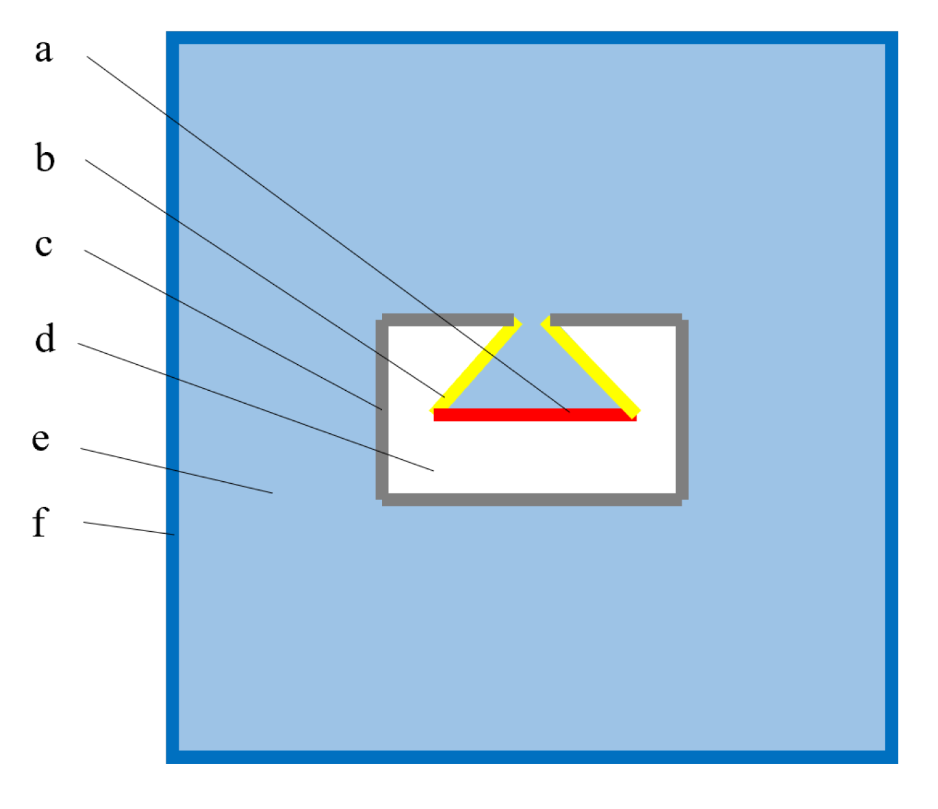
• Boundary conditions. The domain boundary and external cavity are defined at 300 K. The surfaces in the internal cavity, both lateral(steel) and base(copper), were defined as isothermal at various cavity temperatures. The body’s material is incompressible ideal gas (air), with a density of 1.225 kg/m${}^3$, and conductivity of 0.0242 W/m·K. Detailed boundary conditions are illustrated in Figure 9:
• Methods. According to Ansys Fluent Theory Guide 2021R2, the velocity–pressure coupling is treated using the SIMPLE algorithm in the presence of multiple generic models. The pressure is discretized using the PRESTO! Scheme (Fluent Incorporated, 1996). The second-order upwind scheme is used for the momentum and energy terms.
• Calculation. This calculation first utilizes a pressure-based steady time solver with 2000 steps. Then, a transient-time solver is applied with one time step at 0.05 s and 50 iterations each step. The iterative solution is converged when the residuals are below 0.1% for continuity and velocity, and 0.0001% for energy.

An investigation into the reduction in heat losses in cavity receivers is the focus of the heat loss approach. The heat losses from existing cavity designs are also investigated using the CFD method. The CFD results acquired in the numerical solution can be applied to obtain the cavities’ thermal conversion power under specific conditions (incoming radiation, environment, and cavity temperature). Results are listed in Section 5.1.4.

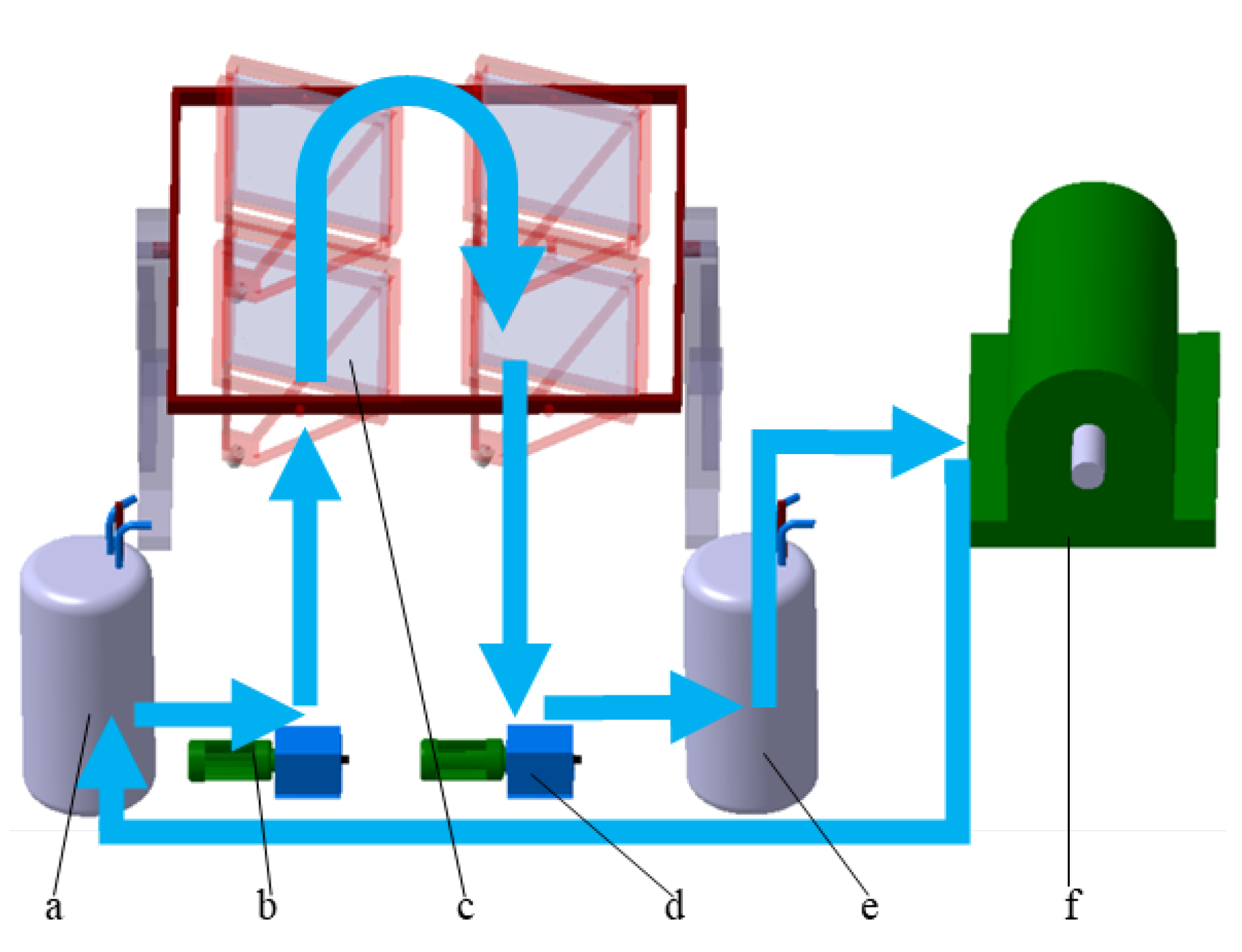
4. Experimental Investigations

The experiment investigated the thermal conversion performance of the novel conical cavity receiver by measuring the workflow’s temperatures at the inlet and outlet of the collector simulation system designed in this research. Then, the heating power can be calculated in an enthalpy course. Afterwards, the heating power in the novel receiver is compared with existing designs.

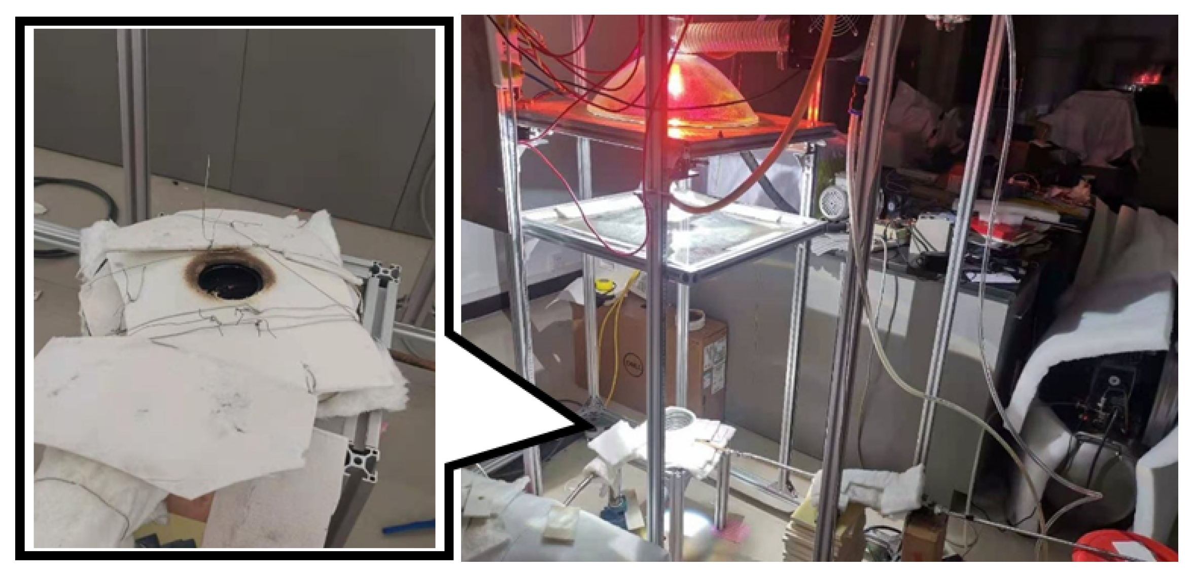
4.1. Experimental System Setup

The collector simulation system generates and concentrates radiation at a constant power into the cavity receiver, where the working fluid absorbs the energy. This system mainly consists of two groups: the concentration system and the receiver–pipeline system.

The concentration system includes an air-cooled 5 kW xenon short arc lamp acting as the point light source (a 5 mm linear light source). The bulb is located at the focus of the parabolic reflector, which is about 400 mm in diameter and 130 mm in depth. Light rays are reflected and turned into collimated rays. They go through a PMMA Fresnel lens and concentrate at the receiver. The flux reaching the receiver is around 1 kW.

The receiver–pipeline system mainly includes the compressor, the cavity receiver, and a variety of valves and gauges. The compressor keeps the work fluid at a range from 0.55 MP to 0.7 MPa in a working cycle. The pressure is stabilized by a reduction valve. The workflow is adjusted by a throttle valve and measured by a volumetric flowmeter after the reduction valve. Then, the working fluid temperature at the inlet and outlet of the receiver is measured by two transmitters. A back-pressure valve is installed to preserve air pressure in the pipeline before the working fluid is discharged at the end of the pipeline. The receiver can be dismounted and replaced by another one in the test.

In the pipeline, most components are connected by braided stainless steel tubes, which have good tolerance of temperature and pressure, and ease of placement. Rigid tubes are applied before and after the flowmeter. For heat insulation, nano-microporous materials with a thermal conductivity of 0.018 W/m·K at 300 K are installed outside the receiver.

The experiment system layout is shown in Figure 10.

The setup of the experiment system is shown in Figure 11.

4.2. Performance Test

Cavities of different geometries were tested. The same volumetric flow and pressure were adopted: 55 L/min and 0.38 MPa. The highest-pressure compressor was 0.38 MPa, and the valves remained constant at room temperature. The temperature at the inlet and outlet of the receiver was measured during the experiment. The enthalpy of the inlet and outlet workflow can be obtained according to the specific temperature and pressure in the literature.

The tested cavities are shown in Figure 12. The length of the copper tube forming one cavity is near 1200 mm.

The temperatures at the inlets and outlets of the cavity receivers were used to calculate the heating power that was directly transferred to the working fluid from the identical light source. The experimental results are listed in Section 5.2.1.

5. Results and Discussion

5.1. Numerical Results

5.1.1. Effect of Dimensions on Thermal Absorption

The heat absorption in the novel positive conical cavities with different apertures and heights, under an identical incoming flux of 1 kW, concentrated by a Fresnel lens, was traced. One example of the traced cavity models is shown in Figure 13. This example’s cavity height and aperture were 15 mm and 45 mm, respectively.

The distribution of heat flux absorption in the above cavity is shown in Figure 14.

The absorption results of cavities of different dimensions are listed in

Table 2. Power absorption of different dimensions *.

	Height/mm	15	25	35	45
Aperture Diameter/mm
$\mathsf{\Phi }$30		836.82	852.05	858.89	862.97
$\mathsf{\Phi }$45		824.54	839.62	848.93	852.70
$\mathsf{\Phi }$60		818.22	834.81	843.74	844.29

* Incoming flux 1 kW concentrated by a Fresnel lens, base diameter 154 mm, base surface absorptance 85%, lateral surface reflectivity 80%, focus adjusted at 0.5 mm intervals.

.

The results show that the differences in the investigated cavities’ heat absorption do not exceed 5.5%. To reduce the system size, a cavity height of 15 mm and aperture diameter of 45 mm are selected according to the high tolerance of dimensions.

5.1.2. Effect of Surface Absorptance on Thermal Absorption

Heat absorption in the selected cavity with different surface absorptances is traced under an identical incoming flux of 1 kW. The results are listed in

Table 3. Power absorption for different surface absorptances *.

Base Absorptance/%	75	80	85	90	95
Power Absorption/W	753.0	789.62	824.54	857.76	873.17
	(−8.7%)	(−4.2%)	–	(+4.0%)	(+5.8%)

* Incoming flux 1 kW, concentrated by a Fresnel lens, aperture diameter 45 mm, base diameter 154 mm, cavity height 15 mm, lateral surface reflectivity 80%, focus adjusted at 0.5 mm intervals.

.

The results show that the cavities’ heat absorption drops by 14% when the surface absorptance drops from 95% to 75%.

High absorptance is feasible for state-of-the art materials and surface treatment; however, their performance may degrade through aging. A surface absorptance of 85% was selected in this research.

5.1.3. Effect of Geometries on Thermal Absorption

The power absorption of negative conical, hemispherical, and cylindrical through cavities was compared with the novel design under the incoming flux of 1 kW. The geometries share an absorption area near 1900 mm${}^2$ and surface absorptance of 85%.

The distribution of heat flux absorption in the cavities in Figure 13 and Figure 15 is shown in Figure 16:

The power absorption in the positive conical, negative conical, hemispherical, and cylindrical through cavities are listed in

Table 4. Power absorption for different geometries (ray tracing) *.

Geometry	Positive conical	Negative conical	Hemispherical	Cylindrical through
Power Absorption/W	824.5	898.4	868.9	643.9

* Incoming flux 1 kW, detailed factors in Figure 16.

. Xie [19] achieved similar results in his numerical comparison of existing designs without consideration of heat loss.

The results show that the novel positive cavity receiver under-performs the negative and conical cavity receivers by a small percentage.

The absorption results should be considered with heat losses to determine the thermal conversion performance of the cavities. The cylindrical through cavity demonstrates a special case, where part of the incoming flux fails to reach the absorber surface; thus, the absorption is far inferior.

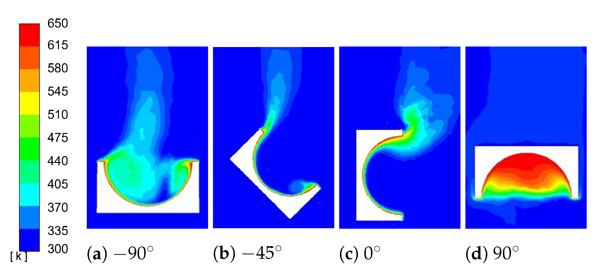
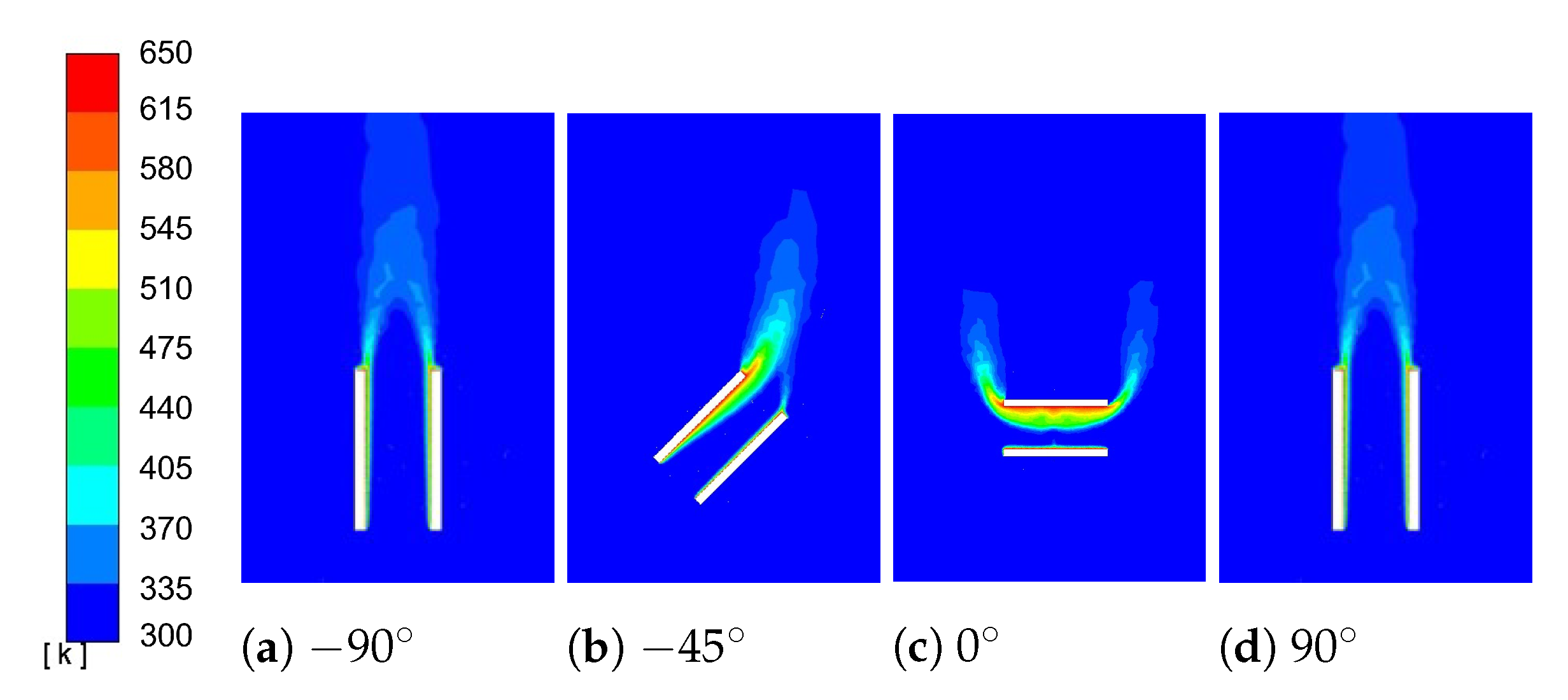
5.1.4. Heat Losses in Cavity Receivers

The positive and negative conical, cylindrical, and hemispherical cavities were analyzed for heat losses at temperature levels ranging from 450 K to 750 K and various inclinations. The inclination is defined according to the parabolic dish systems, so the aperture facing upward is at a −90° inclination. The heat losses with inclination at 90° are exhibited as a reference.

Detailed geometry parameters of the receivers are given in Section 5.1.1 and Section 5.1.3. The CFD configurations are introduced in Section 3.2. Section contour views of the air temperature when the cavities’ surface temperature is 650 K are shown from Figure 17, Figure 18, Figure 19 and Figure 20:

The detailed heat loss numerical results for cavities at different inclinations are summarized in

Table 5. Heat losses in cavities/W.

Inclination/°	Temperature/K	450	550	650	750
−90	Positive conical	3.14	8.26	14.51	25.47
	Negative conical	43.81	98.97	177.20	290.80
	Hemispherical	45.90	94.67	175.26	291.93
	Cylindrical through	31.8	63.87	107.20	166.18
−45	Positive conical	7.90	15.69	25.37	37.74
	Negative conical	47.50	101.58	183.87	300.78
	Hemispherical	49.68	107.35	189.24	309.05
	Cylindrical through	31.38	63.20	106.34	165.05
0	Positive conical	7.75	15.59	25.39	37.92
	Negative conical	44.11	96.31	175.16	290.94
	Hemispherical	44.17	96.52	175.52	291.44
	Cylindrical through	27.52	56.65	97.14	153.14
90	Positive conical	1.74	4.79	9.87	18.06
	Negative conical	31.16	96.35	147.15	254.89
	Hemispherical	33.56	76.45	150.20	259.96
	Cylindrical through	31.8	63.87	107.20	166.18

.

The heat loss results show that the positive conical cavity has a significant heat loss reduction compared with existing designs at the same cavity temperature and inclination.

5.1.5. Thermal Conversion in Cavity Receivers

After deducting the heat losses in Table 5 from the absorption results in Table 4 to calculate the thermal conversion power, the results at different inclinations are listed in

Table 6. Thermal conversion in cavities/W.

Inclination/°	Temperature/K	450	550	650	750
−90	Positive conical	821.36	816.24	809.99	799.03
	Negative conical	854.59	799.43	721.20	607.60
	Hemispherical	823.00	774.23	693.64	576.97
	Cylindrical through	612.10	580.03	536.70	477.72
−45	Positive conical/K	816.60	808.81	799.13	786.76
	Negative conical	850.90	796.82	714.53	597.62
	Hemispherical	819.21	761.56	679.66	559.85
	Cylindrical through	612.52	580.70	537.56	478.85
0	Positive conical	816.75	808.91	799.11	786.58
	Negative conical	854.29	802.09	723.24	607.46
	Hemispherical	824.73	772.38	693.38	577.46
	Cylindrical through	616.38	587.25	546.76	490.76
90	Positive conical	822.76	819.71	814.63	806.44
	Negative conical	867.24	802.05	751.25	643.51
	Hemispherical	835.34	792.45	718.70	608.94
	Cylindrical through	612.10	580.03	536.70	477.72

Incoming flux, 1 kW; surface absorptance, 85%; detailed cavity factors in Figure 16, Figure 17, Figure 18, Figure 19 and Figure 20.

.

The trend of different cavities’ thermal conversion power with a temperature rise is presented in Figure 21.

Due to the inferior absorption, the novel positive conical design underperforms in thermal conversion in comparison with traditional negative conical and hemispherical cavities below 550 K, under the incoming flux of 1 kW. With the temperature rise, the effect of heat loss reduction outweighs the inferior absorption, and the novel cavity realizes and maintains a higher thermal conversion performance. The temperature of 550 K is far below the normal working temperature of CSP facilities, and accessible for almost all state-of-the-art collector system designs.

The cylindrical through cavity is a special case, where the absorption is too inferior to heat the cavity to the temperature needed for the heat losses to take effect. Real field applications usually utilize an alternative cylindrical design.

5.1.6. Validation of Numerical Results

Dimensionless Nusselt numbers are compared in

Table 7. Nusselt number validation.

	This Research * (Numerical)	Research 1 [26] (Numerical)	Research 1 (Experimental)	Research 2 [16] (Numerical)
Nusselt number	13.64	13.50	12.55	14.03

* The hemispherical cavity at the inclination of −90°.

.

The numerical results of the hemispherical cavity (inclination at −90°) are comparable with previous research.

5.2. Experimental Results

5.2.1. Thermal Conversion under Identical Radiation

The inlet and outlet working fluid temperature of different designs were measured at 0.38 MPa, with an inlet volumetric flow rate of 55 L/min. The working fluid was compressed air. The energy was calculated using an enthalpy course according to the temperature rise. Since the focus point was not actually a point, the position of the focus was modified at 10 mm intervals, which could obtain the maximum conversion power for each cavity geometry.

The experimental results are listed in

Table 8. Power conversion for different geometries (experimental).

	Positive Conical	Negative Conical	Hemispherical	Cylindrical Through
Inlet temperature/°C	31.8	29.8	27.1	29.3
Outlet temperature/°C (highest cavity temperature)	223.2	208.3	205.8	141.1
	(411)	(362)	(330)	(185)
Power conversion/W	984.0	920.3	932.1	577.1
	(100%)	(−6.5%)	(−5.3%)	(−41.4%)

Working fluid: compressed air, at 0.38 MPa, 55 L/min; Cavity-forming: copper tubes, external diameter 8 mm, internal diameter 6 mm, black-painted; Insulation: SiO₂ porous nano-material, conductivity at 0.018 W/m·K.

.

The novel positive conical cavity’s thermal conversion outperforms existing designs by at least 5.6% (compared to the hemispherical cavity) in the experimental investigation.

5.2.2. Comparison with numerical results

Before comparing the numerical and experimental results, the following issues are considered:

• The thermal process is not balanced but an instant value in the numerical investigation.
• Heat transfer to the working fluid is not the concern in the numerical investigation or heat loss reduction design.
• The thermal process is balanced under a constant incoming flux, but only thermal conversion is acquired in the experimental investigation.
• The manufactured parts have dimensional errors with numerical models.

The boundary conditions in the numerical investigation are adjusted according to the experimental results. The numerical and experiment results are compared in relative forms in

Table 9. Relative power conversion (% of positive conical cavity).

	Positive Conical	Negative Conical	Hemispherical	Cylindrical Through *
Absorption, numerical/W	824.5 **	898.4 **	868.9 **	534.5 ***
Heat loss, numerical ****/W	25.8	162.5	134.1	27.6
Conversion, numerical/W	798.7	735.9	734.8	506.9
Relative conversion (numerical)/%	100	92.1	92.0	63.5
Relative conversion (experimental)/%	100	93.5	94.7	58.6

* Cavity diameter 50 mm, height 80 mm; ** Detailed parameters in Section 5.1.3; *** Surface absorptance at 85%, incoming source flux at 1000 W, concentrated by Fresnel lens; **** Re-calculated; temperatures adjusted according to Table 8.

:

After reasonable adjustments, the combined numerical and experimental investigations provide comparable results. They study the same thermal process from different aspects and overcome each other’s restraints.

The novel design’s geometry forming is un-optimized planar circular. Thus, the superior performance is due to the heat loss reduction designs, including the reflective lateral surface and reduced aperture.

Both investigations were carried out at relatively low working temperatures compared with state-of-the-art CSP facilities. It can be reasonably expected that this advantage can be maintained as the heat loss growth is more significant than the absorption change with the temperature rise.

6. Conclusions

In this research, the effect of heat loss on the cavity receiver’s conversion efficiency was analyzed. A positive conical cavity receiver scheme is proposed accordingly. This receiver’s solar thermal conversion was numerically investigated using ray tracing and CFD numerical methods. The numerical results were validated using a CSP simulative experiment system designed for this research. This research has the following findings and outcomes:

• The heat loss reduction design approach can be realized by simple measures, with structure improvements that benefit manufacturing, installation, and maintenance.
• The novel cavity design realizes a drastic reduction in heat loss. In this research, at the cavity temperature of 650 K, the heat loss is reduced by as much as 91.8%.
• Although it is not optimized for absorption, the novel design can realize a higher conversion power. In this research, when compared using an identical incoming flux of 1 kW, it outperforms by 5.6%, at least in the experiment setup.
• The heat loss reduction design shows an increase with the temperature rise.
• The heat loss reduction design requires the absorption to be sufficient to heat the cavity to the specific temperature where the heat losses start to take over the thermal conversion.
• Heat loss comparison is an agile method when comparing the relative performance of different cavity receiver designs.
• The limitations of this research include: heat transfer to the working fluid is not specifically studied in this approach. Thus, the balance heat transfer temperature, or the absolute value of the thermal conversion power, cannot be precisely obtained in the numerical analysis.
• Numerical data can be referenced in future optimizations of the novel positive cavity receiver.

References

1. Petela, R. Exergy of Heat Radiation. J. Heat Transf. 1964, 86, 187–192. [Google Scholar] [CrossRef]
2. Jeter, S.M. Maximum Conversion Efficiency for the Utilization of Direct Solar Radiation. Sol. Energy 1981, 26, 231–236. [Google Scholar] [CrossRef]
3. Moynihan, P. Second-Law Efficiency of Solar-Thermal Cavity Receivers; Jet Propulsion Lab., California Institute of Technology: Pasadena, CA, USA, 1983. [Google Scholar]
4. Wright, S.; Scott, D.; Haddow, J.; Rosen, M. The Upper Limit to Solar Energy Conversion. In Proceedings of the Collection of Technical Papers, 35th Intersociety Energy Conversion Engineering Conference and Exhibit (IECEC) (Cat. No.00CH37022), Las Vegas, NV, USA, 24–28 July 2000. [Google Scholar] [CrossRef]
5. Xie, W.; Dai, Y.; Wang, R. Theoretical and Experimental Analysis on Efficiency Factors and Heat Removal Factors of Fresnel Lens Solar Collector Using Different Cavity Receivers. Sol. Energy 2012, 86, 2458–2471. [Google Scholar] [CrossRef]
6. Mao, Q.; Shuai, Y.; Yuan, Y. Study on Radiation Flux of the Receiver with a Parabolic Solar Concentrator System. Energy Convers. Manag. 2014, 84, 1–6. [Google Scholar] [CrossRef]
7. Qiu, Y.; He, Y.L.; Wu, M.; Zheng, Z.J. A Comprehensive Model for Optical and Thermal Characterization of a Linear Fresnel Solar Reflector with a Trapezoidal Cavity Receiver. Renew. Energy 2016, 97, 129–144. [Google Scholar] [CrossRef]
8. Le Roux, W.; Bello-Ochende, T.; Meyer, J. The Efficiency of an Open-Cavity Tubular Solar Receiver for a Small-Scale Solar Thermal Brayton Cycle. Energy Convers. Manag. 2014, 84, 457–470. [Google Scholar] [CrossRef] [Green Version]
9. Pye, J.; Hughes, G.; Abbasi, E.; Asselineau, C.A.; Burgess, G.; Coventry, J.; Logie, W.; Venn, F.; Zapata, J. Development of a Higher-Efficiency Tubular Cavity Receiver for Direct Steam Generation on a Dish Concentrator. AIP Conf. Proc. 2016. [Google Scholar] [CrossRef] [Green Version]
10. Daabo, A.M.; Mahmoud, S.; Al-Dadah, R.K. The Optical Efficiency of Three Different Geometries of a Small Scale Cavity Receiver for Concentrated Solar Applications. Appl. Energy 2016, 179, 1081–1096. [Google Scholar] [CrossRef] [Green Version]
11. Clausing, A. An Analysis of Convective Losses from Cavity Solar Central Receivers. Sol. Energy 1981, 27, 295–300. [Google Scholar] [CrossRef]
12. Clausing, A.M. Convective Losses from Cavity Solar Receivers—Comparisons between Analytical Predictions and Experimental Results. J. Sol. Energy Eng. 1983, 105, 29–33. [Google Scholar] [CrossRef]
13. Leibfried, U.; Ortjohann, J. Convective Heat Loss from Upward and Downward-Facing Cavity Solar Receivers: Measurements and Calculations. J. Sol. Energy Eng. 1995, 117, 75–84. [Google Scholar] [CrossRef]
14. Quere, P.L.; Humphrey, J.A.C.; Sherman, F.S. Numerical Calculation of Thermally Driven Two-Dimentional Unsteady Laminar Flow in Cavities of Rectangular Cross Section. Numer. Heat Transf. 1981, 4, 249–283. [Google Scholar] [CrossRef]
15. Chan, Y.; Tien, C. A Numerical Study of Two-Dimensional Laminar Natural Convection in Shallow Open Cavities. Int. J. Heat Mass Transf. 1985, 28, 603–612. [Google Scholar] [CrossRef]
16. Reddy, K.; Sendhil Kumar, N. An Improved Model for Natural Convection Heat Loss from Modified Cavity Receiver of Solar Dish Concentrator. Sol. Energy 2009, 83, 1884–1892. [Google Scholar] [CrossRef]
17. Reddy, K.; Vikram, T.S.; Veershetty, G. Combined Heat Loss Analysis of Solar Parabolic Dish–Modified Cavity Receiver for Superheated Steam Generation. Sol. Energy 2015, 121, 78–93. [Google Scholar] [CrossRef]
18. Sendhil Kumar, N.; Reddy, K. Comparison of Receivers for Solar Dish Collector System. Energy Convers. Manag. 2008, 49, 812–819. [Google Scholar] [CrossRef]
19. Xie, W.; Dai, Y.; Wang, R. Numerical and Experimental Analysis of a Point Focus Solar Collector Using High Concentration Imaging PMMA Fresnel Lens. Energy Convers. Manag. 2011, 52, 2417–2426. [Google Scholar] [CrossRef]
20. Li, X.; Dai, Y.; Wang, R. Performance Investigation on Solar Thermal Conversion of a Conical Cavity Receiver Employing a beam-down Solar Tower Concentrator. Sol. Energy 2015, 114, 134–151. [Google Scholar] [CrossRef]
21. Issa, O.O.; Thirunavukkarasu, V.; Sudhakar, P. Novel Designs of Cavity Receiver for a Solar Parabolic Dish Concentrator. J. Phys. Conf. Ser. 2021, 2054, 012036. [Google Scholar] [CrossRef]
22. Zhang, Y.; Xiao, H.; Zou, C.; Falcoz, Q.; Neveu, P. Combined Optics and Heat Transfer Numerical Model of a Solar Conical Receiver with built-in Helical Pipe. Energy 2020, 193, 116775. [Google Scholar] [CrossRef]
23. Pye, J.; Coventry, J.; Venn, F.; Zapata, J.; Abbasi, E.; Asselineau, C.A.; Burgess, G.; Hughes, G.; Logie, W. Experimental Testing of a High-Flux Cavity Receiver. AIP Conf. Proc. 2017, 1850, 110011. [Google Scholar] [CrossRef] [Green Version]
24. Chu, S.; Bai, F.; Zhang, X.; Yang, B.; Cui, Z.; Nie, F. Experimental Study and Thermal Analysis of a Tubular Pressurized Air Receiver. Renew. Energy 2018, 125, 413–424. [Google Scholar] [CrossRef]
25. Hu, Y.; Yao, Y. Optical Analysis and Output Evaluation for a Two-Stage Concentration Photovoltaic System by Using Monte Carlo Ray-Tracing Method. Optik 2017, 131, 713–723. [Google Scholar] [CrossRef]
26. Khubeiz, J.M.; Radziemska, E.; Lewandowski, W.M. Natural Convective Heat-transfers from an Isothermal Horizontal Hemispherical Cavity. Appl. Energy 2002, 73, 261–275. [Google Scholar] [CrossRef]
Figure 1. Schematic diagram of the energy flow in the cavity receiver.
Energies 15 00784 g001
Figure 2. Schematic view: the collector module and the conical cavity receiver. (Left): the collector module; (right): section views of the cavity receiver.
Energies 15 00784 g002
Figure 3. Comparison with ASTRI receiver design: (a) Area directly heated by concentrated solar rays; (b) area heated by conductive, convective and radiative energy; (c) highly reflective area, with no heat transferred to working fluid; (d) insulation. (Left): ASTRI 3-D and section view [9]; (Right): The positive conical cavity receiver.
Energies 15 00784 g003
Figure 4. CSP system scheme: (a) normal pressure storage; (b) initial pump; (c) collector system; (d) high temperature pump; (e) high temperature/pressure storage; (f) turbine (and generator).
Energies 15 00784 g004
Figure 5. Cavity designs for analytical investigation: (a) positive conical cavity; (b) negative conical cavity.
Energies 15 00784 g005
Figure 6. Cavity efficiency results in analytical investigation: (a) Cavity exergy conversion efficiency; (b) Cavity energy conversion efficiency.
Energies 15 00784 g006
Figure 7. Ray-tracing scheme for sunlight absorption. (a) Sunlight source, Φ 400 mm, heat flux 1 kW, (b) Fresnel lens, Φ 500 mm, (c) cavity receiver, (c-1) lateral surface for reflection, reflectivity 80%, (c-2) positive conical cavity connecting to ambient air, (c-3) base for absorption, diameter 154 mm, absorptance to be selected.
Energies 15 00784 g007
Figure 8. Section view of meshed body (air).
Energies 15 00784 g008
Figure 9. Section view of boundary conditions: (a) Isothermal copper wall at cavity temperature, conductivity = 387.6 W/m·K; (b) isothermal steel wall at cavity temperature, conductivity = 16.27 W/m·K; (c) isothermal wall at 300K, conductivity = 0; (d) hollow (excluded from calculation); (e) incompressible ideal air, density = 1.225 kg/m 3 , conductivity = 0.0242 W/m·K; (f) pressure inlet, constant gauge pressure = 0, temp = 300 K.
Energies 15 00784 g009
Figure 10. The collector simulation system layout: (a) Air compressor, (b) reduction valve, (c) valve, (d) volumetric flow meter, (e) temperature transmitter, (f) cavity receiver (g) Fresnel lens, (h) parabolic reflector, (i) Xenon lamp, (j) temperature transmitter, (k) back-pressure valve.
Energies 15 00784 g010
Figure 11. Setup of the experiment system.
Energies 15 00784 g011
Figure 12. Tubular cavities of different geometries in the experiment: (a) positive conical *; (b) negative conical; (c) hemispherical; (d) cylindrical through. *: This cavity is formed by two parts.
Energies 15 00784 g012
Figure 13. Positive conical cavity model for numerical ray tracing. (a) Positive conical cavity (base diameter 154 mm, aperture diameter 45 mm, cavity height 15 mm, external diameter 165 mm, external height 20 mm). (b) Positive conical cavity (section view). Red: absorption surfaces, absorptance 85% is selected in this section; Yellow: reflection surface, reflectivity 80%.
Energies 15 00784 g013
Figure 14. Ray tracing and base heat flux. Base diameter 154 mm, aperture diameter 45 mm, height 15 mm, incoming flux 1 kW, concentrated by a Fresnel lens, absorptance 85%, lateral surface reflectivity 80%, focus adjusted at 0.5 mm intervals.
Energies 15 00784 g014
Figure 15. Existing cavity design models for numerical ray tracing: (a) negative conical cavity (base diameter and slant height 110 mm, external diameter 120 mm, external height 100 mm); (b) hemispherical cavity (cavity diameter 110 mm, external diameter 120 mm, external height 60 mm); (c) cylindrical through cavity (cavity diameter 50 mm, height 121 mm, external diameter 60 mm). Red: absorption surfaces; an absorptance of 85% is selected in this section.
Energies 15 00784 g015
Figure 16. Sunlight absorption of different shapes: (a) positive conical (Base diameter 154 mm, aperture diameter 45 mm, base surface absorptance 85%, lateral surface reflectivity 80%); (b) negative conical (aperture diameter and slant height 110 mm, surface absorptance 85%); (c) hemispherical (aperture diameter 110 mm, surface absorptance 85%); (d) cylindrical through (aperture diameter 50 mm, cavity height 121 mm, surface absorptance 85%). Incoming flux 1 kW, focus adjusted at 0.5 mm intervals.
Energies 15 00784 g016
Figure 17. Section temperature contour views of the novel positive conical cavity receiver. Cavity: lateral surface isothermal steel at 650 K, base isothermal copper at 650 K; external receiver surface: isothermal at 300 K, adiabatic; body: incompressible ideal gas, ambient air at 300 K.
Energies 15 00784 g017
Figure 18. Section temperature contour views of the negative conical cavity receiver. Cavity: isothermal copper at 650 K; external receiver surface: isothermal at 300 K, adiabatic; body: incompressible ideal gas, ambient air at 300 K.
Energies 15 00784 g018
Figure 19. Section temperature contour views of the hemispherical cavity receiver. Cavity: isothermal copper at 650 K; external receiver surface: isothermal at 300 K, adiabatic; body: incompressible ideal gas, ambient air at 300 K.
Energies 15 00784 g019
Figure 20. Section temperature contour views of the cylindrical through cavity receiver. Cavity: isothermal copper at 650 K; external receiver surface: isothermal at 300 K, adiabatic; body: incompressible ideal gas, ambient air at 300 K.
Energies 15 00784 g020
Figure 21. Thermal conversion at different inclinations. Identical incoming flux 1 kW, concentrated by Fresnel lens; temperature at 300 K; ambient pressure.
Energies 15 00784 g021