Article

Assessment of the Effectiveness of Photovoltaic Panels at Public Transport Stops: 3D Spatial Analysis as a Tool to Strengthen Decision Making

Faculty of Geodesy and Cartography, Warsaw University of Technology, Pl. Politechniki 1, 00-661 Warsaw, Poland
*
Author to whom correspondence should be addressed.
Energies 2022, 15(3), 1230; https://doi.org/10.3390/en15031230
Submission received: 29 December 2021 / Revised: 1 February 2022 / Accepted: 4 February 2022 / Published: 8 February 2022
(This article belongs to the Special Issue Energy Decision Making: Problems, Methods, and Tools)

Abstract

:
The potential of solar energy encourages research into new applications of this technology. Access to renewable energy is an important element of modern urban policies aimed at sustainable development and the energy security of residents but also limits energy production from conventional sources due to the pollution associated with them. More and more often, projects of new urban infrastructure facilities include integrated photovoltaic panels. Assessing solar potential is an important step when planning the layout of solar panels, and the increasing number of high-rise buildings increases shaded areas, sometimes even for most of the day. Therefore, a detailed shading analysis can be important for city decision makers, investors and local communities. The results of the 3D spatial analysis presented in the article can be used to optimize the location and analyse the profitability of photovoltaic installations in a city. The aim of the project was to evaluate the effectiveness of photovoltaic panels on the shelters of public transport bus/tram stops. The proposed methodology for calculating the solar potential and shading may be a valuable extension of existing solutions in the field of planning installation power and the location of individual panels. The research methodology can be used in the future to support decision making and spatial planning related to the placement of photovoltaic panels. It was tested for bus shelters located in the centre of Warsaw (Poland). The results can also be used to assess the impact of alternatives to newly designed high-rise buildings and to plan the provision of photovoltaic panels to other city infrastructure facilities.

1. Introduction

1.1. Energy Demand of Today’s Cities

It is widely recognised that our cities need a change. However, discussions are ongoing about the direction of these changes. Is a city supposed to constantly accelerate and fully benefit from modern technological solutions, becoming a smart city? Alternatively, should it be adopting a slower pace of change, transforming according to David Sim’s vision [1] to be better adapted to the human scale (a soft city)? This idea has been developed since 2016 by Prof. Carlos Moreno [2,3] and was implemented in the development of Paris (a 15 min city). A modern city is favourable to pedestrians and users of public transport [4], is green and ecological [5], and uses renewable sources to the greatest possible extent [6]. However, due to the growing population in cities [7], the energy demand in these areas is still increasing. The use of conventional sources is associated with air pollution, which in many cities exceeds the acceptable standards many times over, especially in the autumn and winter. The damage caused by combustion products of conventional fuels is currently the greatest threat to the environment and leads to the worsening of the greenhouse effect and the enlargement of zones with high air pollution [8]. This, in turn, has a negative impact on the health of the inhabitants. Urban areas in Poland, Bosnia-Herzegovina, Serbia, and Turkey commonly experience two or more months during which the average air quality is classified as “unhealthy” [9].
The European Union countries undertake many activities to reduce the emissions of harmful substances produced by the energy industry. In December 2019, the European Union reached an agreement to reduce net greenhouse gas emissions by at least 55% by 2030 compared to 1990 levels (“Fit for 55”) [10] and achieve climate neutrality by 2050 [11]. The new vision for the European Union’s development includes activities related to the reduction in CO2 and changes in transport, industry, reduction in emissions from buildings, significant changes in food production technologies, and limiting the loss of biodiversity. The EU is in the process of revising its 2030 greenhouse gas (GHG) emissions reduction target. Various stakeholders from the Member States and EU institutions to civil society have put forth differing thresholds for the greenhouse gas emissions cuts needed to meet the Paris Agreement goals: 50%, 55%, 60%, or 65% [12]. In November 2021, the COP26 (26th UN Climate Change Conference of the Parties) summit concluded with all countries agreeing to the Glasgow Climate Pact. For the first time, it was agreed to phase down unabated coal power and phase out inefficient fossil fuel subsidies [13]. For some participants, it was a major disappointment that a clear decision was not made to phase out fossil fuels altogether, but only to limit them. Only 46 countries (e.g., the UK, Canada, Poland, and Vietnam) made commitments to phase out domestic coal, while a further 29 countries (e.g., the UK, Canada, Germany, and Italy) committed to ending new direct international public support for unabated fossil fuels by the end of 2022 and to redirecting this investment into clean energy. Efforts were also made to scale up solar investment with the launch of a new Solar Investment Action Agenda by WRI, the International Solar Alliance (ISA), and Bloomberg Philanthropies that identifies high-impact opportunities to speed up investment and reach ISA’s goal of mobilizing $1 trillion in solar investment by 2030 [14].

1.2. Solar Energy and Photovoltaic Installations
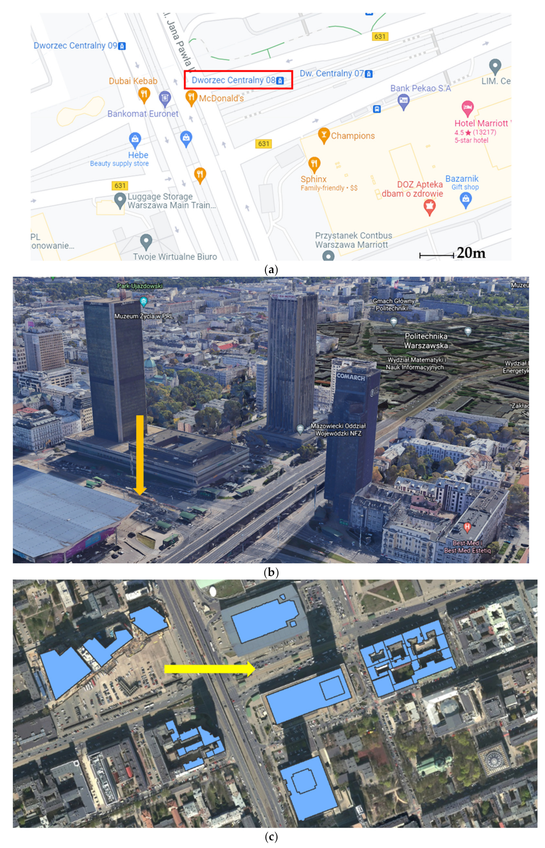
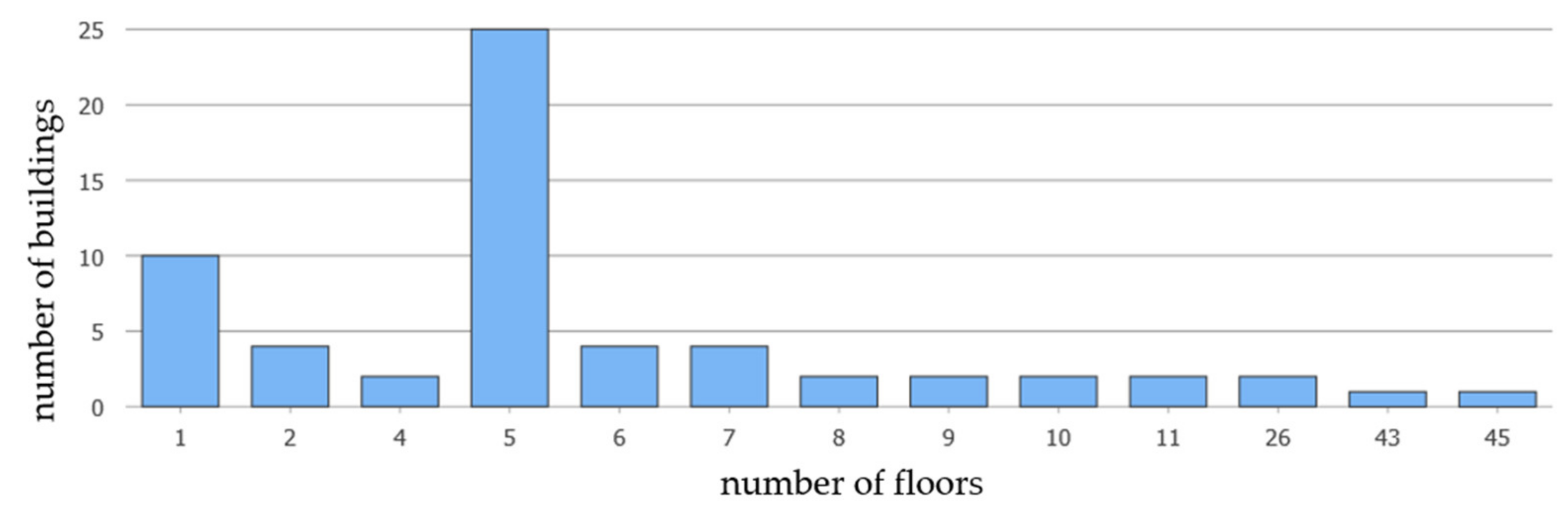
One of the measures currently underway is, therefore, to increase the share of renewable energy in the energy market [15,16]. The Global Energy Review 2021 emphasized that renewable energy use increased 3% in 2020 as demand for all other fuels declined. Solar PV and wind are set to contribute two-thirds of renewable growth [17]. Photovoltaics (PV) is a key technology option for realising a decarbonised power sector and sustainable energy supply. There is a noticeable increase in investments, including in photovoltaics in the public and private market [18].
One of the challenges of the cities of the future is to increase the area intended for photovoltaic installations. Private companies, nongovernmental organizations, and cities are already investing in photovoltaics. Residents are also encouraged to carry out such installations on their own. Many systems have been created, e.g., the so-called “solar cadastre” and geoportals of many cities, so it is possible to determine the potential profitability of installing solar panels on one’s own roof or in the backyard. The scope of the data provided by such portals is different and the information that can be obtained is also different. It may be information about the potential class of the whole roof (e.g., in Amsterdam [19] or London [20]), e.g., specifying conditions on a scale from very favourable to unfavourable; data on individual roof slopes (e.g., in Geneva [21] or Vienna [22]); continuous distribution of suitability within the roof on a conventional scale (e.g., Vienna [22], Google Sunroof [23]), or in kWh/m2/year (Luxembourg [24]). These are both 2D visualizations (e.g., Frankfurt [25], Helsinki [26], and Amsterdam [19]) and 3D (e.g., Vienna [27] and Helsinki [26]), presenting roof data in vector format (e.g., Geneva [21] and London [20]), raster format (e.g., Amsterdam [19] and Luxembourg [24]), or as a grid of points placed on the roofs of buildings (e.g., Boston [28]). Some of them also allow us to obtain data for the ground surface (e.g., Frankfurt [25]), but there are also those that allow us to assess the suitability of individual walls of buildings (e.g., Helsinki [26] and Vienna [27]). Most of the portals allow us to generate a report for a given building or location, providing information on the energy possible to obtain yearly (often divided into individual months); some also provide possible financial profits depending on the estimated power of the installation (e.g., Google Sunroof [23], New York [29], and Osnabrück [30]) and the saved CO2 emissions or obtained energy, divided into direct and diffuse radiation (e.g., Helsinki [26]). The most advanced tools allow for manual or automatic design of the distribution of panels within the roof area (e.g., Luxembourg [24]).
Various types of installations can be distinguished depending on how the panels are installed: ground mount PV systems (GPV), rooftop PV systems (RPV), or building-integrated photovoltaics (BIPV). There are also agrivoltaic systems (APV) that avoid the competition between land use for installations and agricultural land use, reduce evaporation, and provide shade-loving crops from excessive heat [31]. Thanks to the latest technology, which is constantly being improved, in the near future it will be possible to obtain energy regardless of the time of day, which may be a breakthrough in the photovoltaic market [32]. The next step to ensuring the energy security of cities may be not only equipping buildings with photovoltaic installations, but also planning urban infrastructure integrated with solar panels and using appropriate tools to support making such decisions. It is important to plan new investments so that they have the greatest possible solar potential. One can find in the literature examples of 3D analysis carried out for the roofs of buildings [33,34,35,36,37] also taking into account mutual shading [38]. However, little attention is paid to other elements of the urban infrastructure. In the literature, there are few examples of installing PV on other city infrastructure such as the cooling towers in power plants [39], sewage facilities, bridges, solar carports, or bus shelters [40,41]. An example of such a solution is the photovoltaic bus shelters operating in London [42], Paris [43], San Francisco [44], Singapore [45], and Turin [41], as well as in Poland in Rzeszów and Stalowa Wola [46]. The obtained energy is used, among other things, to power digital displays and timetables, to power the WiFi network, and to charge mobile phones free of charge, as well as for cooling in summer and heating in winter. Despite the continuous development of the spatial information infrastructure, access to data, and the implementation of advanced algorithms, city decision-makers do not fully use the possibilities of advanced tools to support decision making in the field of planning and expanding the infrastructure of renewable energy resources. The above analysis was the genesis of the research presented in this article.
The current trend toward the maximum use of urban space and the resulting increase in the number of skyscrapers in downtown areas causes an increase in shaded areas for many hours during the day. It is, therefore, important to plan the location of solar panels so that energy losses due to shading are as low as possible. This problem is particularly important in areas away from the equator (Figure 1), where energy gains when the sun is low above the horizon are much lower. In Poland, this potential varies only (on average, daily) from 2.6 kWh in the northwest to 3.2 kWh in the southeast of the country (Figure 2). The amount of energy supplied varies considerably with the seasons of the year. In winter, it may be sevenfold less than in summer. About 77% of the annual radiation energy is obtained from April to September, and only 23% from October to March. The sunniest months in Poland are June–August, when about 43% of the annual radiation is obtained [47]. A threat related to the amount of energy reaching the surface, which results directly from the location of Poland, may be the instability of the weather, which has been increasing in recent years [48].
One of the factors may be cloud cover, i.e., the degree of sky coverage by clouds, which is determined by the octant scale from 0 (sky without clouds) to 8 (full cloud cover).
In 2018–2020, among the stations conducting the research, the lowest cloudiness was recorded in Suwałki (2.2 octans in April 2019) and Ustka (2.5 octans in May 2018). The highest cloudiness was recorded for the station in Suwałki (7.5 octans in December 2018 and 7.3 octans in November 2019) [50]. On such days, even with clearing, the energy production is much lower. Regardless of these conditions, however, photovoltaic energy seems to be a favourable solution in Poland, although not as beneficial as in other regions of the world [51]. According to data from the Energy Market Agency, the installed capacity of photovoltaics in Poland was, at the end of September 2021, nearly 6.3 GW. This means an increase of 100.3% compared to September 2020 [52].

2. Research Area

Research assessing the efficiency of photovoltaic panels was carried out for two selected tram stops along with their surroundings located in the Śródmieście district and on the border of the districts: Śródmieście and Wola. The locations were in the centre of Warsaw (the capital), due to the intensive development of high-rise buildings, which causes a continuous increase in the shading of the surroundings. The comparison of the two locations made it possible to verify the correctness of the selected methodology and to take into account the influence of local factors on the results of the analysis. The first location is the Rondo ONZ 04 tram stop. The stop is located on Aleja Jana Pawła II at Rondo ONZ, close to the second metro line station, and is surrounded by high-rise buildings, the location of which is shown in Figure 3. It is used by lines 10, 11, and 14, which run north of Warsaw. From there, there are 378 trams a day, which means that trams leave the stop every 3 min on average during the working week [53]. Figure 4 shows the number of buildings in the vicinity of the stop and the number of their storeys, ranging from 1 to 45 floors. These include Ilmet, Rondo 1, Kaskada, and Atrium. At the time of the project implementation, the SKYSAWA skyscraper was not yet put into operation. Plans for this location include at least two more skyscrapers, including Warsaw One, the shape of which is already included in this project. Taking into account the designed building will reflect the real situation in this location in the near future, and the height of the building about 80 m higher than the existing office building in this place will significantly extend the shadow cast [54]. The second location is the Dworzec Centralny 08 tram stop, located near the main railway station in the city centre, serving long-distance journeys (Figure 5). It is used by lines 7, 9, 22, 24, and 25, which head to the southwest of Warsaw. There are 589 trams running from it daily on a weekday, so departures take place approximately every 2 min during the working week [55]. There are also high-rise buildings in the immediate vicinity of this shelter. An example is the LIM Center at Aleje Jerozolimskie Steet (the total height of the skyscraper is 170 m), and at the intersection of Chałbińskiego Street and Chmielna Street, the tallest building in the European Union (Varso Place) is being built; ultimately, it is to reach a height of 310 m. The planned completion date was estimated to be at the beginning of 2022 [56]. The building of the central station, located at Aleje Jerozolimskie Steet, in the immediate vicinity of the selected stop, may have little impact on the solar radiation reaching this place due to the relatively low height and the location on the northern side of the shelter being analysed. Figure 5 shows an orthophotomap of the vicinity of the Central Railway Station with the buildings selected for analysis, while Figure 6 presents the number of buildings and the number of their storeys, also in the range from 1 to 45 floors.

3. Materials and Methods

3.1. Source Data

For many planning tasks, the standard two-dimensional presentation is sufficient, but the introduction of a third dimension can provide important new information about objects—not only information about the position, but also about its shape and attributes, for example: the height, number of floors (in the case of a building), the geometry of the roof, etc. In 2002, members of the Special Interest Group 3D began working on the creation of a semantic information model that would represent 3D objects in such a way that they could be used by various applications (City Geography Markup Language, CityGML) [57]. Successive levels of modelling detail in CityGML have been defined, from simple models without topologies to complex ones with detailed semantics. There are five levels of LoD detail, as shown in Figure 7. The LoD0 model is a 2.5-dimensional representation of the numerical terrain model, while the LoD1 model assumes a generalized building geometry, i.e., flat roofs of buildings (the so-called solid model). In LoD2, models of buildings with a roof structure (real mapping of roofs) are presented. On the LoD3 level, buildings are presented in more detail than on the LoD2 level, with all the elements present, while LoD4 complements LoD3, taking into account the interior of the building [58].
In Poland, the Central Office of Geodesy and Cartography (GUGiK) made available 3D models of buildings created by combining three data sources: 2D outlines of buildings from the BDOT10k database (a reference database of topographic objects with an accuracy corresponding to an analogue map of 1:10,000); elevation data from airborne laser scanning technology (ALS) with a density of 12 points/m2 in urbanized areas; and data from the digital terrain model (DTM) in raster form with a spatial resolution of 1 m × 1 m. The models were created in the CityGML 2.0 standard at the level of detail LoD1 and LoD2 [59] and are available for general use, free of charge. More detailed data (LoD2) are available for the study area described in Section 2.
The next set of data was a polygon layer containing the ground floor contours of buildings from the Database of Topographic Objects (BDOT10k) (a reference database of topographic objects with an accuracy corresponding to an analogue map of 1:10,000). These data have been made available by GUGiK for general use, free of charge. The locations of public transport stops (point layer) and bus shelters (polygon layer) were obtained from the database of the open OSM project.
The control of the validity of the obtained data showed that some buildings (outlines of buildings and 3D solids) were not included in the acquired datasets. These objects had to be created manually, using an aerial orthophotomap provided by the WMS service of Warsaw [59]. Digital surface model (DSM) data were generated from Airborne Laser Scanning (ALS) source data; point clouds had a scanning density of 12 points/m2. These data were obtained via the ISOK project [60] and have been made available by GUGiK for general use, free of charge.
Climatic data are taken into account when determining solarization conditions; these come from the NASA research program Surface meteorology and Solar Energy (SSE) database and have been compiled from satellite data. They include long-term estimated quantitative data on the flow of solar energy on the Earth’s surface. The database is available on the project website and contains sufficiently accurate data that it is possible to cover areas where measurements are rarely performed or not performed at all [61,62]. Additionally, the free SoDa data were used [63]. The website allows one to generate solar radiation time series based on data from the HelioClim-1 satellite. The satellite provides monthly, weekly, and daily data for 1985 to 2005. The result is generated in CSV format, thanks to which it was possible to obtain a long-term monthly average in the form of a table [64].

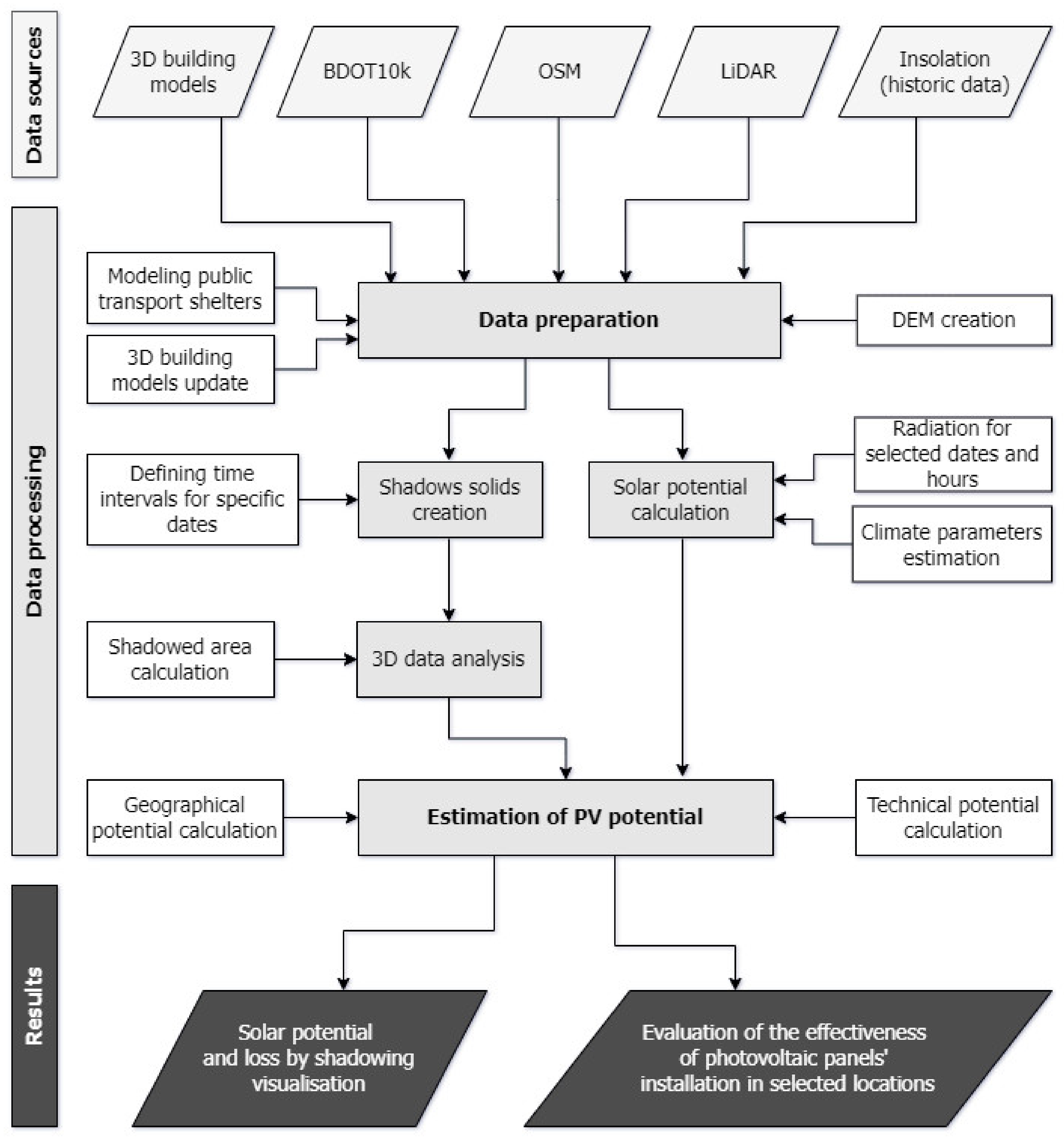
3.2. Methods of Processing and Analysis

In this project, a spatial analysis is proposed to estimate solar energy losses as a result of shading for selected locations in the centre of Warsaw and to assess the effectiveness of photovoltaic panels installed on shelters of public transport stops. It was necessary to take into account the solar radiation reaching the selected locations and the potential shading, as well as a number of factors that have a direct impact on the amount of energy produced, i.e., on the efficiency of the installation (Figure 8).
The data flow diagram presented in Figure 9 visualizes the process of obtaining a result from the source data, as well as the relationship between successive variables of the process. In the first stage, the data for analysis was acquired. These data required initial processing or manual supplementation (in the case of 3D building models). Next, two key transformations took place, i.e., the creation of the shadow volumes (solids) and the calculation of the solar potential. It should be noted here that, for the established detail of the data and the parameters adopted in the study, the calculations were time-consuming. Therefore, a number of preliminary tests were performed to select the optimal settings.
The presented scheme of processing was automated as a script in Python (Python Software Foundation, Wilmington, DE, USA) using the ArcPy library in the ArcGIS environment. All data processing algorithms used were originated from ArcGIS Desktop 10.7.1 software (Esri, Redlands, CA, USA).

3.2.1. Data Preparation for Analysis

Before conducting the appropriate spatial analysis, the source data had to be properly preprocessed. On the basis of the available metadata [65], the bus shelters were given appropriate roof dimensions and a height of 2.5 m. This height corresponds to the dimensions of the shelters, which are currently installed in Warsaw, both at the ONZ roundabout and at the Central Station. Then they were transformed into 3D objects (solids). Since the data collected in the GUGiK resource were obtained, new office buildings and apartment buildings were built in both analysed locations due to the dynamically changing landscape of the city. As mentioned before, some investments are still planned or under construction. As the implemented and planned investments are not included in spatial databases, for the purposes of the analysis, the acquired database of buildings was updated with the shapes of missing skyscrapers in order to assess the shading status as accurately as possible in the near future.
These buildings are presented in the form of solids at the level of detail LoD1, but this generalization (no exact shape of the roof) does not have a significant impact on the modelling results, so this difference was considered insignificant for the purposes of this project. The visualization of the final dataset is presented in Figure 10 and Figure 11.
The digital terrain model (DTM) in raster format is the required data source for the analysis of the solar potential. Only points from class 2 (ground) were selected to create a numerical terrain model from the ALS measurement data [66]. The binning interpolation method was used to create DTM. This is a point aggregation method commonly used in the processing of high-density point clouds to raster format [67]. It is faster than triangulation and is the recommended solution in the literature [68]. The last important parameter is the spatial resolution of the DSM raster used in the analysis to perform calculations for the roof of the bus shelters. Before choosing the appropriate resolution, different variants of the size of this parameter had to be tested. Based on the literature [69,70,71,72,73] and taking into account the size of the research area and the roof area of the bus shelter, the following spatial resolutions were considered during the analysis: 0.5 m, 0.25 m, 0, 20 m, 0.15 m, 0.1 m, and 0.05 m.

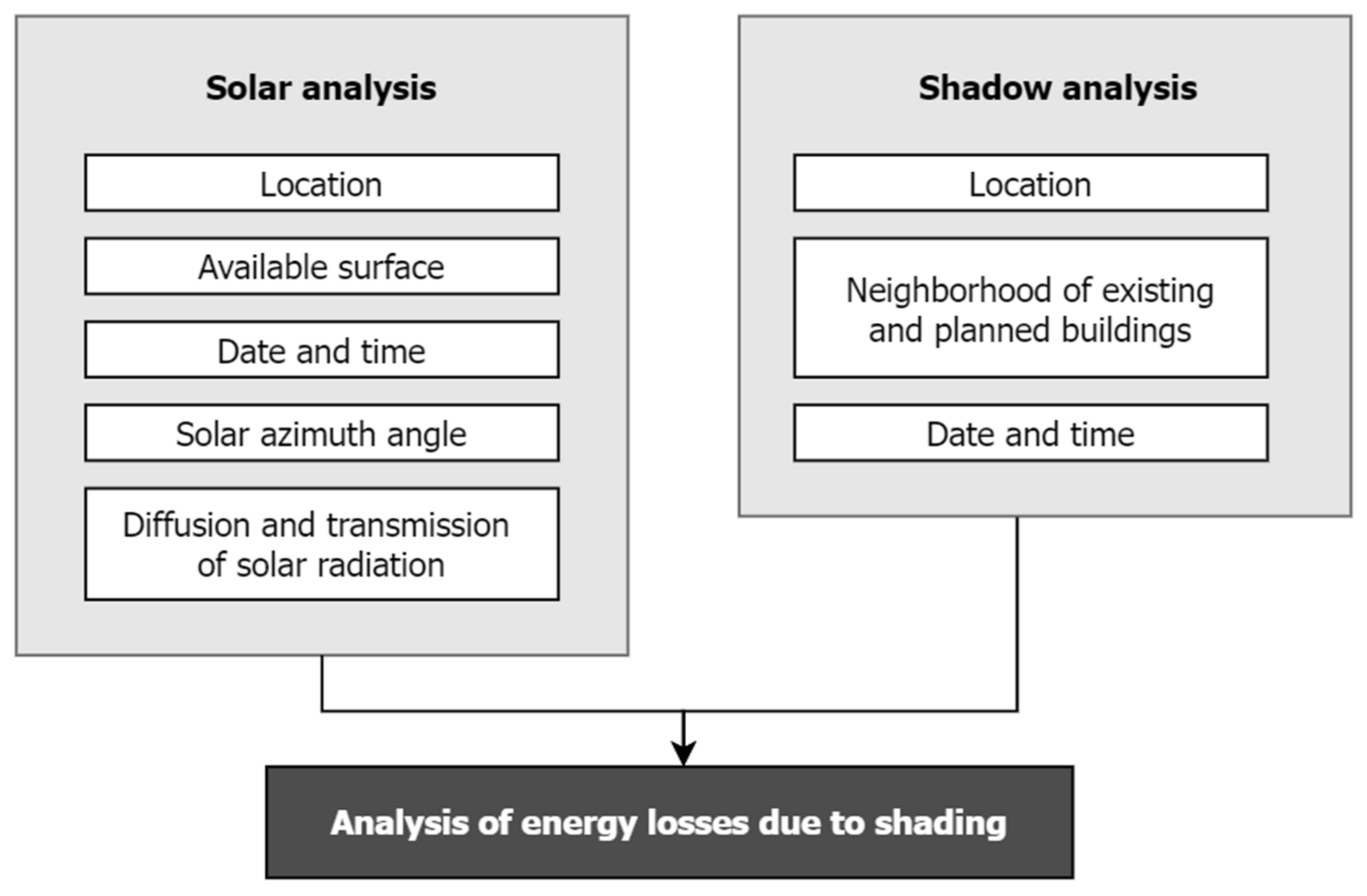
3.2.2. Solar Analysis

For the purposes of the analysis, two characteristic dates were adopted for the calculations, the days of the summer and winter solstices (22 June 2020 and 22 December 2020); for the two months adopted, historical data were acquired. Using the SSE and SoDa services, the average monthly values of daily solar radiation for June and December for the area of the centre of Warsaw were generated (latitude = 52.23° N, longitude = 21.00° E). An albedo coefficient of 0.25 was adopted for the radiation calculations. It was calculated on the basis of the average of the coefficients for urbanized areas based on the literature [74]. The average monthly daily solar radiation (kWh/m2) for the centre of Warsaw in June and December is shown in Figure 12. There are significant differences in values between the seasons, from about 150–170 kWh/m2 in June to an average of less than 20 kWh/m2 in December.
Two key algorithms were used to carry out solar analysis: to calculate the solar potential (Area Solar Radiation, ASR) and to model shadows cast by selected objects (Sun Shadow Volume, SSV). The amount of solar radiation reaching the Earth’s surface depends to a large extent on the topography and land cover. Therefore, the digital surface model (DSM) data, as well as slope maps and aspect maps, are used to calculate the solar potential.
The ASR tool calculates the insolation based on the semicircular viewshed model [75,76], which can be determined for any location. This algorithm uses a view from the observation point that resembles a semicircular shot of the Earth in a photograph aimed at the sky, which gives the impression of a view like in a planetarium. A key role is played by the size of the fragment of the uncovered sky that allows the radiation to reach the Earth (in observation point). A graphic representation of the visible part of the sky is determined, taking into account any obstacles that may limit the amount of radiation reaching the tested location. First, it computes horizontal angles in a specified number of directions within the selected location (Figure 13a).
In the next step, interpolation of the angles on the horizon is performed for the directions in between those defined in the previous step. As a result, a 2D raster image is created, which contains information about the degree of obstruction of the sky by obstacles, as shown in Figure 13b (the visible part of the sky is shown in white, and the invisible part in grey). Figure 13c shows a combination of the obtained result and a semicircular photograph (view in all directions). Solar radiation falling directly on the Earth’s surface is computed using a sun map, mapped in the same way as the sky obscuration model. The sun map is represented by a raster image that shows the changes in the position of the sun depending on the hour and month for which the calculations are made. This map consists of discrete intervals (sectors) defined by the position of the sun at a specific time of the day. The path that the sun apparently traverses is determined based on the latitude of the analysis area and the dates and times that define the individual sectors. Thus, the incident direct radiation is calculated for each sector. To calculate the radiation that is scattered before reaching the Earth’s surface, an all-sky map visible from a given location must be created. This map is segmented afterwards using zenith angles and azimuths. Both described maps are shown in Figure 14 (the colours are given randomly in the visualization and are only intended to emphasize the extents of individual sectors).
To calculate the value of insolation, the sky obscuration model is superimposed on the sun map (Figure 15a) and the sky map (Figure 15b), with the products obtained in the previous stage. In the first step, for both cases, the proportion of the visible sky in each sector is calculated, which is the result of dividing the number of visible cells by the number of all raster cells per sector. Finally, the value of solar radiation is the sum of the direct and diffuse radiation values.
The ASR algorithm uses the sky resolution parameter for the sky shading model, sun map, and sky map; the default value is 200 cells. When calculating the sky shade, a parameter is used that determines the number of azimuth directions. Values must be multiples of 8 (for example, 8, 16, 24, 32, etc.). The default value is 32 directions, which is appropriate (recommended) for terrains with a complex topography. The next parameters used to create a sky map are the number of divisions with respect to the zenith and the number of divisions with respect to the north direction (azimuth divisions). In both cases, the default value is 8. It is also possible to select the scattered radiation model: uniform sky (the scattered radiation is the same from every direction) or standard overcast sky (the diffuse radiation beam varies with the angle to the zenith). Important parameters in the calculations are also diffuse proportion and the permeability of the atmosphere, which is the part of radiation that passes through the atmosphere (transmittivity). Both parameters can take values from 0 to 1. The default scattering value for a cloudless sky is 0.3, while the transmittance of the atmosphere, assuming a clear sky, is 0.5. The main result of the ASR algorithm is a raster representing the total radiation (in Wh/m2) calculated for each point of the input layer. In addition, it is possible to generate raster images containing information on direct radiation (in Wh/m2), scattered radiation (in Wh/m2), and duration of direct solar radiation (in h).
As described in Section 3.2.1, further versions of the DTM with spatial resolution from 0.5 m to 0.05 m were created using the source ALS data. Then, on the basis of each variant of the resulting DTMs, maps of the solar potential were created to compare the obtained values. The tests were performed for the area of the Rondo ONZ 04 tram stop neighbourhood on June 22, for the hours from 11:00 to 12:00 at 15 min intervals. Appropriate transformations were performed for each resolution to obtain a result in the form of a map of the solar potential for the roof area of the bus shelter. The obtained results show that the value of the radiation intensity changes significantly with the change in the spatial resolution of performed calculations, which proves that at a higher spatial resolution the results are more precise. For further processing, it was decided to use the DTM spatial resolution equal to 0.1 m in order to obtain optimally detailed description for the analysed object (bus shelter) with an acceptable processing time (approximately 13 h for one bus shelter using Intel® Core™ i5-3337U CPU @ 1.80 GHz processor (San Francisco, CA, USA) and 4.00 GB RAM).
The last step of this stage was to calculate the correct solar potential values using the ASR algorithm. On the basis of the obtained results, the insolation values for the bus shelters were calculated (Figure 16).

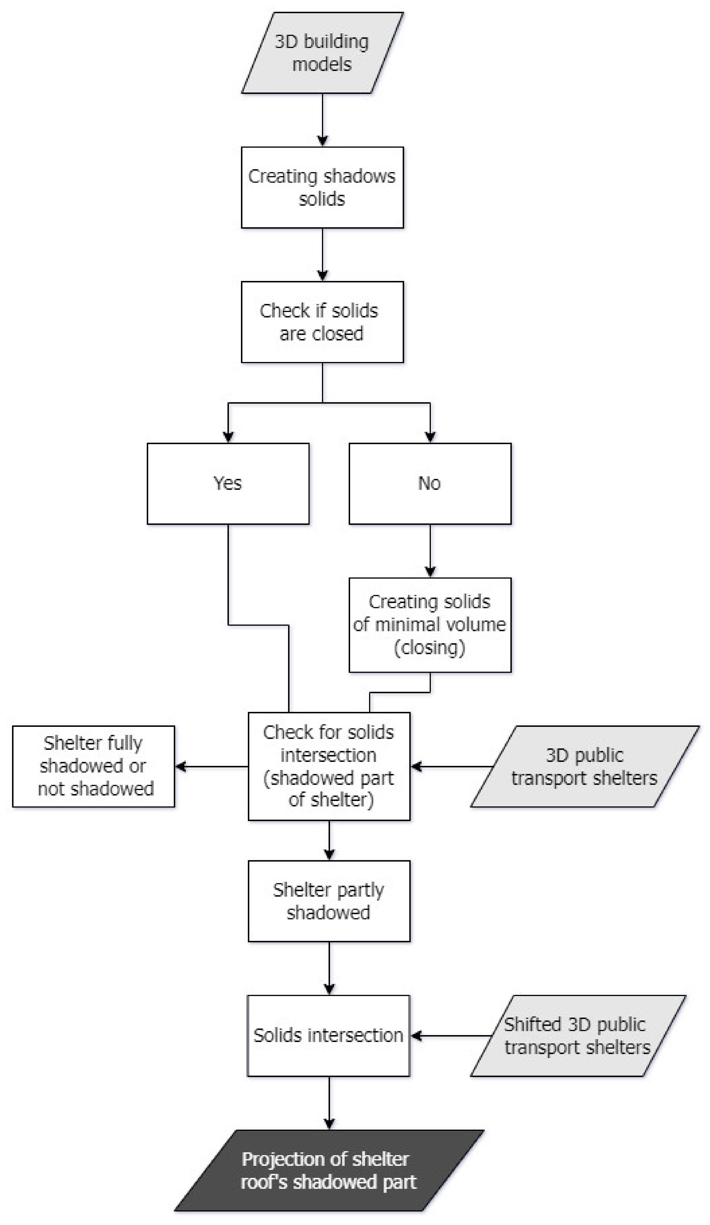
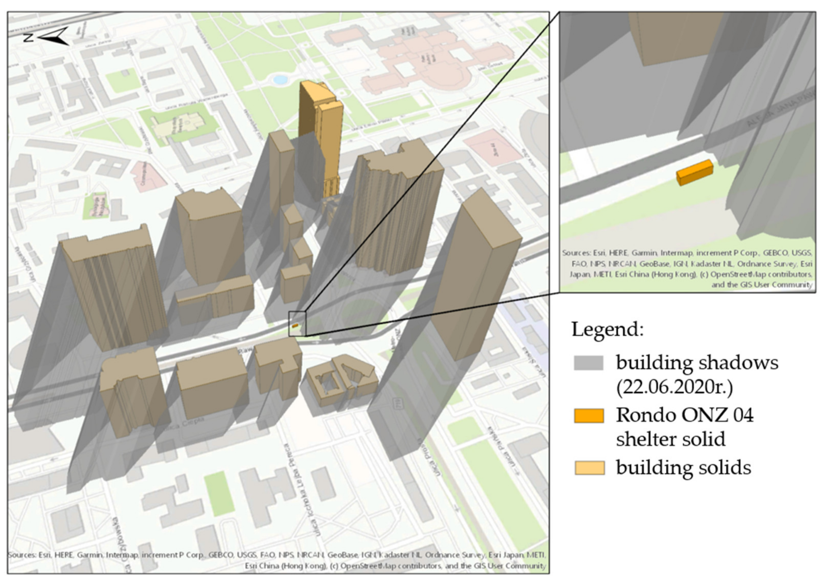
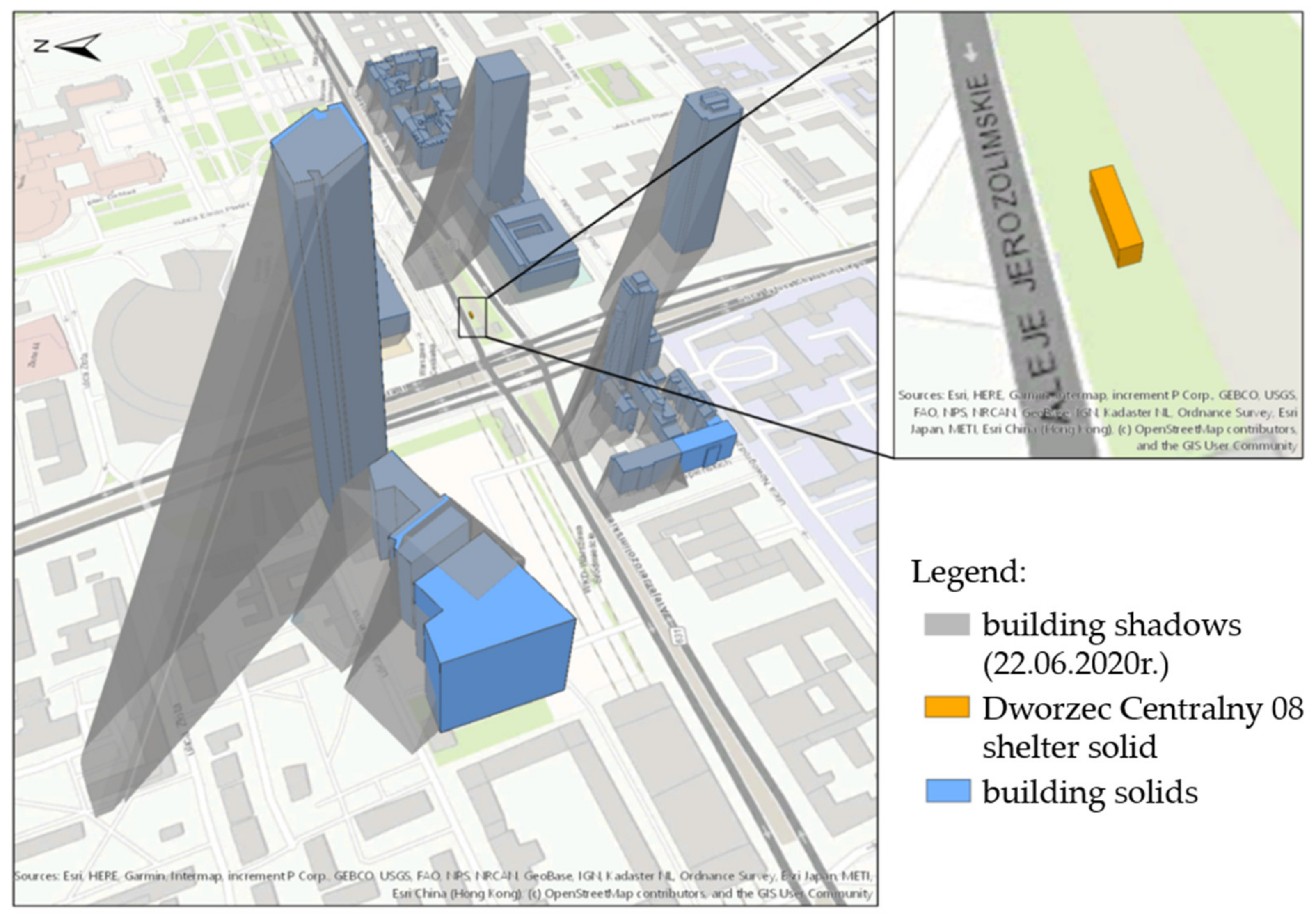
3.2.3. 3D Spatial Analysis

Modelling buildings in 3D not only allowed for a completely new level of visualization and data mining in the third dimension but also enabled a complex 3D analysis. It is possible to obtain information on what part of the space is occupied by the shadow being cast (3D solid) and the trace of the shadow cast on the Earth’s surface (3D polygon). With such data, it is much easier to make decisions [78], as the shadows cast by tall objects on solar panels can cause large reductions in the amount of energy supplied—even partial shading can significantly reduce the overall efficiency of the installation [79]. To properly generate shadows, a 3D algorithm is needed. The algorithm takes into account the geographical location of the observation site and the given day of the year and given time for which the shadow is to be determined. Objects are classified as shaded where the 3D shadow solid intersects the 3D solid of the object (when there is a nonzero intersection of both datasets). In the methodology of creating a solar atlas in Berlin, shadows cast by vegetation, tall buildings, and other objects protruding above the ground were also generated. Moreover, each significantly shaded part of the roof was considered unsuitable for PV installations and was not taken into account during further analysis [80].
The 3D shadow models in the project were generated using the Sun Shadow Volume (SSV) algorithm. The process consists of creating solids that are 3D representations of the shadow areas cast by individual objects for a specific shading object position, date, and time. Shadow modelling involves “pressing” the initial data in the direction of incidence of the sun’s rays, which are parallel to each other, and their direction is calculated on the basis of the relative position of the sun. Each solid has its beginning and end in a vertical plane that is perpendicular to the horizontal projection of the sun’s rays [81]. Figure 17 shows the shadows generated in the morning hours for a selected day in March.
The parameters of the SSV algorithm are the day and time the calculations (shadow generation) start and the day and time the calculations are to be completed. The interval unit is directly related to the aforementioned parameters. It defines the time interval for which the shadows are to be generated (days, hours, or minutes). Another parameter is used to define the time zone and set the time (Daylight Savings Time, DST). The presented methodology also uses tools for assessing geometric properties and relations between 3D objects: Inside 3D (checks whether a given object is contained in another object in whole or in part); Is Closed (to control a possible problem with the solids being not closed); Minimum Bounding Volume (to create a 3D object that represents a solid with a minimum volume “spanned” on the input data); and Intersect 3D (to create an intersection of the analysed solids).

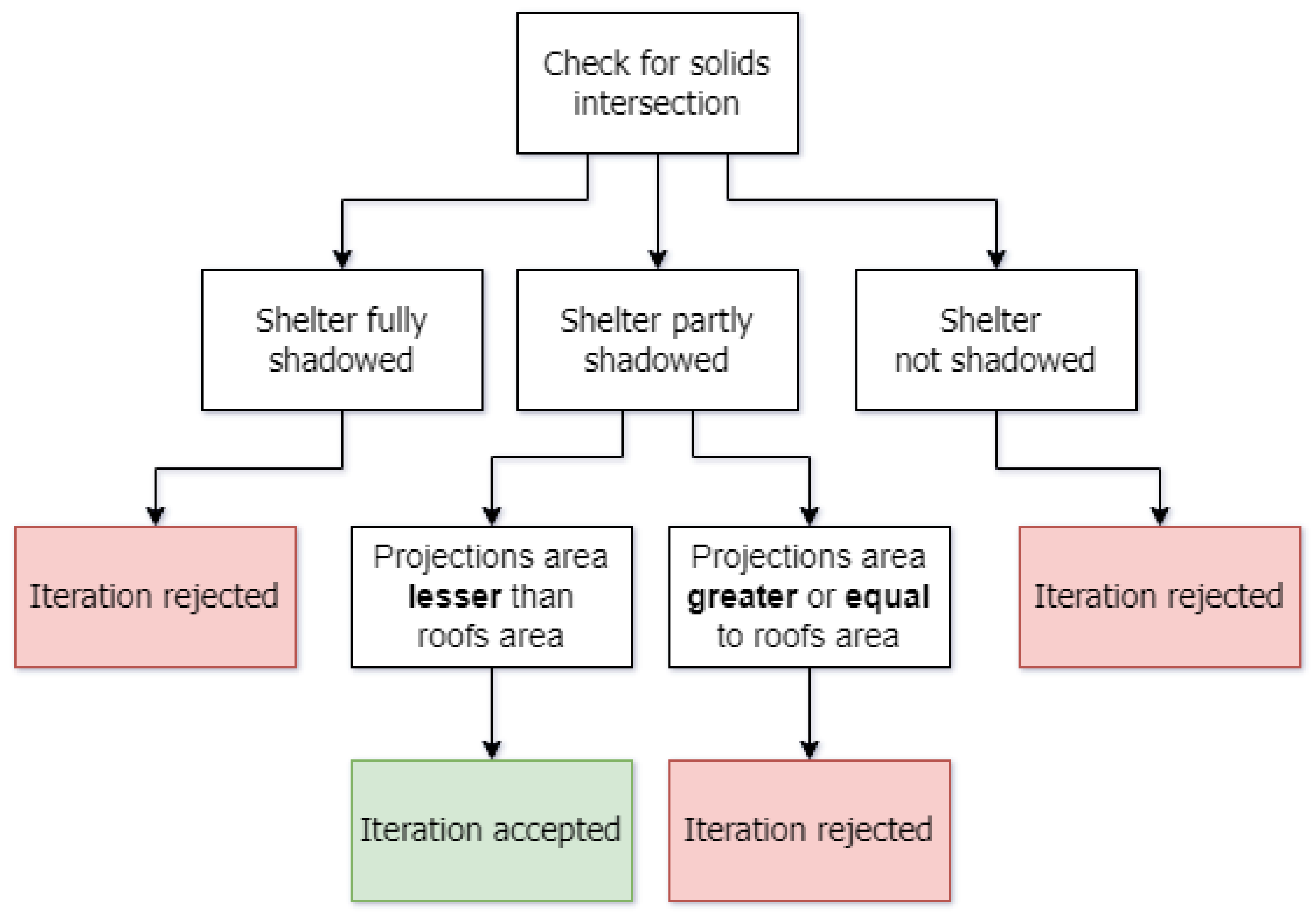
3.2.4. The Influence of Shading on the Solar Potential of Tram Shelter Roofs

The aim of this stage was to obtain the result in the form of polygons that fit into the outline of the shelter roof, reflecting the sunny and shaded fragments.
Figure 18 shows a diagram of the workflow performed during 3D analysis. The process of creating the projection of the shaded and sunny parts of the shelter roofs on the horizontal plane was fully automated using a Python script. Thanks to this, it was possible to quickly determine the area of sunny and shaded parts, determining the shading time with appropriate detail (calculations with a 5 min interval). During the analysis of the changes in the position of the shadow shapes for the selected interval, it was possible to analyse the shadow movement over the observed time.
The shadows were generated for two selected days of the year: 22 June and 22 December. The calculations were made for the entire range of hours from sunrise to sunset. Figure 19 shows the shadows generated in June for buildings around the tram stop Rondo ONZ 04 at 10:30, while Figure 20 shows the shadows of buildings at the Dworzec Centralny 08 tram stop for the same day and time.

4. Results

After the shadows were created, the position of the tram shelter solid and the solids of shadows cast by the buildings were compared. There were three possible types of relations between the shadows cast by the buildings and the roof of the bus shelter: no shadow influence, partial shading, or complete shading. Depending on the case, a different scenario of spatial analysis was implemented, as shown in the diagram (Figure 21). In order to determine the period of no shading, partial, or total shading, we checked the overlapping of the solids and thus calculated the degree of shading and insolation of the shelter for subsequent intervals. In addition, it was necessary to consider the situations when the intersection of the solids took place, but the common part did not contain a shelter roof. These specific possibilities are visualized in Figure 22 (partial shading).
Objects with partial shading were classified to the next step. They were crucial in the further analysis because they carried significant information about the change in the shade of the shelter at specific times, which has a direct impact on the change in the amount of solar energy supplied to this area. The remaining cases were unambiguous. In the case of partial shading, the two scenarios mentioned earlier had to be considered again (the common part can include the roof or not). This variant was solved in the last stage, i.e., after the projection of the shaded part of the shelter roof onto the ground surface. The result of this part of the processing was a solid trace reflecting a fragment of the shed shelter roof. Based on the spatial analysis performed, four sets of graphs (two tram stops and two dates) were developed showing the solar potential in kWh per shelter roof, as well as the percentage loss due to shading and the actual solar potential (including shading). The presented visualizations were created in the form of polar charts. In the next stage, the technical potential was calculated, and the efficiency of photovoltaic panels was assessed.
The results presented in Figure 23, Figure 24, Figure 25 and Figure 26 were obtained by performing the calculations for each day separately. Four measurements were calculated for each hour, reflecting 15 min intervals. For this, the pie slices in the charts consist of four parts, each part representing a 15 min interval. For example, for the interval 10:00–11:00 a.m., the inner segment of the ring corresponds to the range from 10:00 a.m. to 10:15 a.m., the second (counting from the centre) corresponds to the range from 10:15 a.m. to 10:30 a.m., the third reflects the interval from 10:30 a.m. to 10:45 a.m. and the outer segment of the ring is in the range from 10:45 a.m. to 11:00 a.m. The colours in the graphs correspond to the different ranges of the values (see the legend of each chart) in relation to the 15 min interval, and the four segments of the rings (from the centre to the outside) marked in the graphs represent the values of the intervals in the range of the entire hour. In each set, (a) shows the theoretical solar potential, without taking into account the shading, and the units given are expressed in kWh per stop shelter roof area; (b) shows the percentage loss due to shading of the shelter; and (c) shows the actual solar potential, taking into account the shading; the unit is kWh per stop shelter roof area.
When analysing the solar potential for the bus shelter roof at Rondo ONZ 04 in June, it can be noticed that values above zero were recorded between 4:45 a.m. and 7:00 p.m. (Figure 25). The highest values occurred for the hours of 11:45–12:00 p.m. and 12:00–12:15 p.m., providing a total of over 3.8 kWh. The highest percentages of shading of the canopy roof were after sunrise and before sunset: from 7:00 a.m. to 10:00 a.m. and 5:30 p.m. to 9:15 p.m. Little or no shading was observed during the day. Assuming that there were no buildings or other objects in the neighbourhood of the Rondo ONZ 04 tram stop, the sum of the theoretical solar potential for the roof of the selected shelter in June would be approximately 61.0 kWh. Adjusted for the effects of shading by buildings, it is approximately 46.6 kWh.
For the shelter roof at Dworzec Centralny 08 stop in June, solar potential above zero was recorded, similarly to the Rondo ONZ 04 stop, between 4:45 a.m. and 7:00 p.m. (Figure 23). The highest values were recorded between 11:45 a.m. and 12:15 p.m. Due to the differences in area between the stops Rondo ONZ 04 and Dworzec Centralny 08, there were also noticeable differences in the maximum values of solar potential values. At Dworzec Centralny 08, this value was lower, 3.1 kWh in total. When analysing the percentage shading of the shelter roof, it can be seen that it was greatest in the morning between 8:00 a.m. and 9:00 a.m. and in the evening, before sunset, between 7:00 p.m. and 8:15 p.m., but did not occur during the day. The sum of the solar potential in June for the shelter roof of Dworzec Centralny 08 tram stop, assuming no shading, would be about 49.8 kWh; taking into account shading, it was about 44.1 kWh. The loss due to shading was therefore much lower than for Rondo ONZ 04 tram stop.
In December, the highest values of solar potential for the shelter roof of Rondo ONZ 04 were recorded between 10:00 a.m. and 11:00 a.m. (Figure 26). At 10:30 a.m.–10:45 a.m. the sum of the potential was 0.4 kWh, almost fivefold lower than in June at 12:00 p.m.–12:15 p.m., when this value was the highest. Due to the fact that in winter the radiation reaches the surface only between 7:45 a.m. and 1:30 p.m., the sum of the solar potential for the roof was approximately 5.4 kWh, more than 11-fold lower than in June. It could be noted that the shelter is shaded most of the day (assuming the day starts at sunrise and ends at sunset). The sum of the solar potential in December for the shelter Rondo ONZ 04 tram stop, taking into account the shading, was 2.33 kWh.
Figure 24 shows the solar potential for the shelter of Dworzec Centralny 08 tram stop in December. The distribution of ring segments on the graph resembles the December result for the shelter of Rondo ONZ 04 tram stop, and the sum of the values, assuming no shading, was 4.4 kWh. The loss from shading was greatest after sunrise by 10:00 a.m. and from 1:00 p.m. to sunset. This stop can only receive energy for three hours a day. Including the shadows, the sum of the solar potential was approximately 2.8 kWh for the entire shelter roof.
The sum of energy including shadows against the theoretical potential was the highest in June for the stop Dworzec Centralny 08 and amounted to 89% of the theoretical value. For the stop at Rondo ONZ 04 on the same day, it was 77%. In December, the efficiency was lower for both locations: for the shelter of Dworzec Centralny 08 stop it was 66%, and for the shelter of Rondo ONZ 04 it was 43% of the theoretical value. For the shelter of Rondo ONZ 04 in June, the technical potential was over 6.8 kWh, while in December it was only 0.3 kWh. For the shelter of Dworzec Centralny 08, similar results were obtained, despite the greater influence of shadows cast by the surrounding buildings for the shelter of Rondo ONZ 04. In June, for the roof area of the shelter in this location, over 6.4 kWh was obtained, and in December 0.4 kWh. Assuming that the stop equipment would be similar to the city of Corona [83] and the energy consumption would be 1.5 kWh per day, in June the energy surplus for Rondo ONZ 04 stop would be almost 5.3 kWh, and for Dworzec Centralny 08 stop, the surplus would be 4.9 kWh. This energy could be put into circulation and power the traffic light network in the neighbourhood of stops or other infrastructure elements, increasing the level of pedestrian safety (it’s planned to rebuild the intersection at Warsaw Central Station to facilitate pedestrian crossing without underground passages). In December, the generated energy would not be sufficient to power all the facilities installed at the bus stop, so it would be necessary to use the power grid resources, but about 20–30% of the energy would still come from the sun.

5. Discussion

The analysed calculations were presented only for two selected days in the year; such a limitation on the dates was associated with limitations on the time-consuming preparation and control process used in the data analysis, as well as the entire sequence of spatial analysis resulting from the methodology proposed in this work. This limitation does not seem to be an obstacle to the project, which could be implemented, for example, on the order of the authorities of the city of Warsaw. In the future, we might consider adding other 3D shading objects, including tall vegetation, large-format advertising posters, viaducts and footbridges over streets, and other structures. All these objects may have a significant impact on the shading analysis results, as these objects can play an important role in shading bus shelters.
The highest efficiency was achieved for the shelter roof of Dworzec Centralny 08 tram stop in June, and the lowest for the shelter roof of Rondo ONZ 04 stop in December. Its efficiency was 20 times lower than in summer for the shelter of Dworzec Centralny 08 stop. The installation of photovoltaic panels on the roof of the shelter, with the assumptions given in the paper, would obtain over fourfold more energy in summer than the potential demand of the facilities installed at the tram stop, while in winter this energy would be insufficient to power them—the produced energy would constitute 22.5% of the daily demand. Due to the extreme results for two selected days of the year, an interesting continuation of the research would be to find the cutoff days when the installation of panels begins (in spring) and ceases to be profitable (in autumn). Such simulations, also taking into account other shading objects that can cause significant losses in the amount of generated energy, would allow for the optimal selection of the location and type of photovoltaic panels used, as mentioned by Alam et al. [84].
In 2020, Santos et al. presented a solution for bus shelters, carrying out an analysis using raster format data and algorithms [85]. The analysis of the cast shadows is difficult, so the Direct Irradiance Fraction (DIF) was used to describe the amount of insolation that an array will capture (as a percentage), relative to what an optimally oriented, unshaded array would capture in the same location. The advantage of such a solution is the speed of calculations possible on such a data format. In the article from 2021, Gastelu et al. also performed potential calculations for representative blocks of the city, using parallelepipeds to model single-floor houses, two-floor houses, and tall buildings or cylinders and spheres to model trees. They also compared the technical potential values calculated with and without the shading effect, using a shading reduction factor [86].
The assessment of solar potential is an important issue when planning the deployment of photovoltaic panels, which are becoming an increasingly popular source of energy on the Polish market. The proposed methodology can be valuable when planning the installation capacity and the location of individual panels. Given the rapid growth of cities and the increasing number of high-rise buildings, assessing the solar potential along with a shading analysis can be important for city decision makers, transport infrastructure managers, investors, and local communities. The implementation of the proposed workflow and making it available in the form of easy-to-use tools that could function with open or limited access will significantly facilitate decision making about planned solar installations in the city. City reports, planning documents, and strategies can be steered using the specific, reliable results of the analysis. The obtained results can also be used to analyse the profitability of photovoltaic installations related to other infrastructure elements. City managers could require designers of high-rise buildings and city infrastructure to submit data in a three-dimensional form and appropriate data format, to conduct a similar assessment as proposed in this article. The presented solution can also be used as a tool for assessing the different shelter and solar panel options. A similar analysis would allow one to choose the optimal location and size of the public transport shelters.
A limitation of the present research is that the research areas have similar climatic conditions. Cities in Poland do not differ that much, and we do not have access to data of appropriate accuracy and detail for a city with significant climatic differences from Warsaw. This should be taken into account in future studies. On the other hand, our methodology is reproducible for other climatic zones; one only needs to adjust the parameters of the solar analyses to the observation site. From the point of view of methodology development, this seems to us a less important research question.
A possible further research direction is to also consider the type of photovoltaic cell (e.g., mono-, multi-, or a-Si solars) and see how shading affects the efficiency depending on the type of installation. Apart from that, it is worth undertaking in further research the subject of the influence of assumed albedo values on parameters of applied algorithms and results of spatial analyses in absolute terms and in comparative analyses between selected months.
We decided to limit the analysis to two dates: 22 June and 22 December. This meant that the results reflected extreme conditions; considering more dates would certainly help with the analysis of variability in the study area. Given the time-consuming nature of the analyses performed, these two dates seemed sufficient. It is certainly worth considering the inclusion of further dates in further research in this area to obtain more detailed results. A possible limitation of the proposed solution is that the proposed methodology uses the tools of the commercial GIS environment; considering the limited access to these tools, it is worth considering open-source software libraries in the future.

6. Conclusions

The aim of the project was to develop a methodology to assess the effectiveness of the location of photovoltaic panels on the roofs of public transport stop shelters. As part of the tests, analyses were performed for two stops surrounded by high-rise buildings: Rondo ONZ 04 and Dworzec Centralny 08. To achieve the goal, appropriate data were collected and prepared, and a series of data processing and complex analysis were designed and carried out, using appropriately selected tools. A methodology combining solar and 3D analysis was proposed. By taking into account the existing buildings and buildings planned for construction in the neighbourhood of the studied areas, the shading that may occur after their construction was assessed.
Based on the conducted analysis, the results of solar potential for the roofs of the tram shelters were obtained throughout the day, at 15 min intervals, as well as the percentage energy loss caused by the shading of the stops by the surrounding buildings. The combination of the sum of the solar potential with the loss made it possible to assess how much solar energy could be obtained during the day on 22 June and 22 December.
It is worth supporting the decision-making processes with the results of this type of analysis at the investment design stage (e.g., a bus shelter, single-family home, etc.), so that when planning photovoltaic installations, one can optimize the shape and slope of the roof or other element on which installation of panels is planned so that their efficiency is as high as possible. Even if we commonly use perovskites (keeping in mind the problems related to time stability and industrialization that still exist) or tandems based on perovskites and silicon solar cells in the future, an analysis will be needed to optimally arrange new types of photovoltaic cells that are integrated, for example, with the facade of buildings. Carrying out such an analysis for an entire city would allow for selecting the most advantageous locations for the initial stage of a new solar photovoltaic investment. We believe that the proposed methodology is universal, but, of course, how the geographical location will affect the parameters of solar analyses and their proper selection must be considered in analyses for other locations.

Author Contributions

Conceptualization, A.F., K.W. and J.C.; methodology, A.F., K.W. and J.C.; software, K.W. and A.F.; validation, A.F.; formal analysis, K.W. and A.F.; investigation, A.F. and K.W., resources, K.W. and A.F.; writing—original draft preparation, A.F.; writing—review and editing, A.F.; visualization, K.W.; supervision, J.C. All authors have read and agreed to the published version of the manuscript.

Funding

This research received no external funding.

Institutional Review Board Statement

Not applicable.

Informed Consent Statement

Not applicable.

Data Availability Statement

The data used in this study are publicly available: 3D building models, Digital Surface Model (DSM) and BDOT10k database (a reference database of topographic objects): https://mapy.geoportal.gov.pl/ (accessed on 17 November 2021); Solargis historic data: https://solargis.com/maps-and-gis-data/download/world (accessed on 17 November 2021).

Conflicts of Interest

The authors declare no conflict of interest.

References

  1. Sim, D.; Gehl, J. Soft City: Building Density for Everyday Life; Island Press: Washington, DC, USA; Covelo, CA, USA; London, OH, USA, 2019. [Google Scholar]
  2. La Ville du Quart D’heure: Pour un Nouveau Chrono-Urbanisme. Available online: https://www.latribune.fr/regions/smart-cities/la-tribune-de-carlos-moreno/la-ville-du-quart-d-heure-pour-un-nouveau-chrono-urbanisme-604358.html (accessed on 17 November 2021).
  3. Introducing the 15-Minute City Project—15-Minute City. Available online: https://www.15minutecity.com/blog/hello (accessed on 17 November 2021).
  4. Middleton, J. Walking in the City: The Geographies of Everyday Pedestrian Practices. Geogr. Compass 2011, 5, 90–105. [Google Scholar] [CrossRef]
  5. Wu, X.; Zhang, J.; Geng, X.; Wang, T.; Wang, K.; Liu, S. Increasing Green Infrastructure-Based Ecological Resilience in Urban Systems: A Perspective from Locating Ecological and Disturbance Sources in a Resource-Based City. Sustain. Cities Soc. 2020, 61, 102354. [Google Scholar] [CrossRef]
  6. Bagheri, M.; Shirzadi, N.; Bazdar, E.; Kennedy, C.A. Optimal Planning of Hybrid Renewable Energy Infrastructure for Urban Sustainability: Green Vancouver. Renew. Sustain. Energy Rev. 2018, 95, 254–264. [Google Scholar] [CrossRef]
  7. UN. Population Division. The World’s Cities in 2018 Data Booklet; UN: New York, NY, USA, 2018. [Google Scholar]
  8. Maziarz, P.; Harasim, E. Wpływ Konwencjonalnych i Niekonwencjonalnych Źródeł Energii Na Środowisko Naturalne. Екoнoмічні Іннoвації 2014, 58, 192–198. [Google Scholar]
  9. Empowering the World to Breathe Cleaner Air | IQAir. Available online: https://www.iqair.com/world-air-quality-report (accessed on 10 November 2021).
  10. EU’s Plan for a Green Transition—Consilium. Available online: https://www.consilium.europa.eu/en/policies/green-deal/eu-plan-for-a-green-transition/ (accessed on 10 November 2021).
  11. A European Green Deal | European Commission. Available online: https://ec.europa.eu/info/strategy/priorities-2019-2024/european-green-deal_en (accessed on 10 November 2021).
  12. Stainforth, T. The EU Climate Target: What’s in the Numbers? Available online: https://ieep.eu/uploads/articles/attachments/3fb9b35e-8d67-4b11-8c8a-a7050f3d7640/EU%20climate%20target%20-%20What’s%20in%20the%20numbers%20(IEEP%202020).pdf?v=63777144458 (accessed on 17 November 2021).
  13. CMA. Glasgow Climate Pact (Draft Version CMA.3). In Proceedings of the Conference of the Parties Serving as the Meeting of the Parties to the Paris Agreement: Third Session, Glasgow, UK, 31 October–12 November 2021. [Google Scholar]
  14. Mountford, H.; Waskow, D.; Gonzalez, L.; Gajjar, C.; Cogswell, N.; Holt, M.; Fransen, T.; Bergen, M.; Gerholdt, R. COP26: Key Outcomes from the UN Climate Talks in Glasgow. Available online: https://www.wri.org/insights/cop26-key-outcomes-un-climate-talks-glasgow (accessed on 21 November 2021).
  15. King, L.C.; Van Den Bergh, J.C.J.M. Implications of Net Energy-Return-on-Investment for a Low-Carbon Energy Transition. Nat. Energy 2018, 3, 334–340. [Google Scholar] [CrossRef] [Green Version]
  16. Green, M.A. How Did Solar Cells Get So Cheap? Joule 2019, 3, 631–633. [Google Scholar] [CrossRef] [Green Version]
  17. IEA. Global Energy Review. 2021. Available online: https://iea.blob.core.windows.net/assets/d0031107-401d-4a2f-a48b-9eed19457335/GlobalEnergyReview2021.pdf (accessed on 21 November 2021).
  18. Jäger-Waldau, A. PV Status Report 2019, EUR 29938; JRC113626; Publications Office of the European Union: Luxembourg, 2018; ISBN 978-92-79-97465-6. Available online: https://www.researchgate.net/profile/Arnulf-Jaeger-Waldau/publication/334389609_PV_Status_Report_2018/links/5d26e31f458515c11c24f143/PV-Status-Report-2018.pdf (accessed on 17 November 2021). [CrossRef]
  19. Zonnepanelen Amsterdam. Available online: https://maps.amsterdam.nl/zonnedaken_erfgoed/ (accessed on 17 November 2021).
  20. London Solar Opportunity Map. Available online: https://maps.london.gov.uk/lsom/ (accessed on 17 November 2021).
  21. Cadastre Solaire de Genève—arx-iT. Available online: https://sitg-lab.ch/solaire/ (accessed on 17 November 2021).
  22. Wien Umweltgut. Available online: https://www.wien.gv.at/umweltgut/public/grafik.aspx?ThemePage=9 (accessed on 17 November 2021).
  23. Project Sunroof. Available online: https://sunroof.withgoogle.com/ (accessed on 17 November 2021).
  24. Énergie—Geoportal Luxembourg. Available online: https://map.geoportail.lu/theme/energie?version=3&zoom=19&X=682315&Y=6379035&lang=fr&rotation=0&layers=1813-2138&opacities=1-1&bgLayer=basemap_2015_global (accessed on 17 November 2021).
  25. Solarkataster Hessen. Available online: https://www.gpm-webgis-12.de/geoapp/frames/index_ext2.php?gui_id=hessen_sod_03 (accessed on 17 November 2021).
  26. Solar Energy Potential. Available online: https://kartta.hel.fi/3d/solar/#/ (accessed on 17 November 2021).
  27. Solarpotenzial3D. Available online: https://www.wien.gv.at/solarpotenzial3d/#/shadow (accessed on 17 November 2021).
  28. Mapdwell Solar System | Boston, MA Solar Map. Available online: https://mapdwell.com/en/solar/boston (accessed on 17 November 2021).
  29. NY Solar Map. Available online: https://nysolarmap.com/ (accessed on 17 November 2021).
  30. Solardachpotenzial Osnabrück. Available online: http://geo.osnabrueck.de/solar/ (accessed on 17 November 2021).
  31. Barron-Gafford, G.A.; Pavao-Zuckerman, M.A.; Minor, R.L.; Sutter, L.F.; Barnett-Moreno, I.; Blackett, D.T.; Thompson, M.; Dimond, K.; Gerlak, A.K.; Nabhan, G.P.; et al. Agrivoltaics Provide Mutual Benefits across the Food–Energy–Water Nexus in Drylands. Nat. Sustain. 2019, 2, 848–855. [Google Scholar] [CrossRef]
  32. Deppe, T.; Munday, J.N. Nighttime Photovoltaic Cells: Electrical Power Generation by Optically Coupling with Deep Space. ACS Photonics 2019, 7, 1–9. [Google Scholar] [CrossRef]
  33. Khan, J.; Arsalan, M.H. Estimation of Rooftop Solar Photovoltaic Potential Using Geo-Spatial Techniques: A Perspective from Planned Neighborhood of Karachi—Pakistan. Renew. Energy 2016, 90, 188–203. [Google Scholar] [CrossRef]
  34. Mutani, G.; Todeschi, V. Optimization of Costs and Self-Sufficiency for Roof Integrated Photovoltaic Technologies on Residential Buildings. Energies 2021, 14, 4018. [Google Scholar] [CrossRef]
  35. Ruiz, H.S.; Sunarso, A.; Ibrahim-Bathis, K.; Murti, S.A.; Budiarto, I. GIS-AHP Multi Criteria Decision Analysis for the Optimal Location of Solar Energy Plants at Indonesia. Energy Rep. 2020, 6, 3249–3263. [Google Scholar] [CrossRef]
  36. Mansouri Kouhestani, F.; Byrne, J.; Johnson, D.; Spencer, L.; Hazendonk, P.; Brown, B. Evaluating Solar Energy Technical and Economic Potential on Rooftops in an Urban Setting: The City of Lethbridge, Canada. Int. J. Energy Environ. Eng. 2019, 10, 13–32. [Google Scholar] [CrossRef] [Green Version]
  37. Boulahia, M.; Djiar, K.A.; Amado, M. Combined Engineering—Statistical Method for Assessing Solar Photovoltaic Potential on Residential Rooftops: Case of Laghouat in Central Southern Algeria. Energies 2021, 14, 1626. [Google Scholar] [CrossRef]
  38. Liang, J.; Gong, J.; Zhou, J.; Ibrahim, A.N.; Li, M. An Open-Source 3D Solar Radiation Model Integrated with a 3D Geographic Information System. Environ. Model. Softw. 2015, 64, 94–101. [Google Scholar] [CrossRef]
  39. Qi, L.; Jiang, M.; Lv, Y.; Yan, J. A Celestial Motion-Based Solar Photovoltaics Installed on a Cooling Tower. Energy Convers. Manag. 2020, 216, 112957. [Google Scholar] [CrossRef]
  40. Mah, D.N.Y.; Wang, G.; Lo, K.; Leung, M.K.H.; Hills, P.; Lo, A.Y. Barriers and Policy Enablers for Solar Photovoltaics (PV) in Cities: Perspectives of Potential Adopters in Hong Kong. Renew. Sustain. Energy Rev. 2018, 92, 921–936. [Google Scholar] [CrossRef]
  41. Mutani, G.; Vodano, A.; Pastorelli, M. Photovoltaic Solar Systems for Smart Bus Shelters in the Urban Environment of Turin (Italy). In Proceedings of the 2017 IEEE International Telecommunications Energy Conference (INTELEC), Broadbeach, QLD, Australia, 22–26 October 2017. [Google Scholar] [CrossRef] [Green Version]
  42. London Transparent about Its New Solar Bus Shelters. Available online: https://newatlas.com/london-polysolar-transparent-solar-bus-shelter/42735/ (accessed on 18 November 2021).
  43. The Multi-Faceted Bus Shelters of Paris | JCDecaux Group. Available online: https://www.jcdecaux.com/blog/multi-faceted-bus-shelters-paris (accessed on 18 November 2021).
  44. San Francisco Bus Shelters—Radius Displays; [Data/Information/Map] Obtained from the “Global Solar Atlas 2.0, a Free, Web-Based Application Is Developed and Operated by the Company Solargis s.r.o on Behalf of the World Bank Group, Utilizing Solargis Data, with Funding Provided by the Energy Sector Management Assistance Program (ESMAP). Available online: http://www.radiusdisplays.asia/products/san-francisco-bus-shelters/ (accessed on 18 November 2021).
  45. Singapore May Have Designed the World’s Best Bus Stop—Bloomberg. Available online: https://www.bloomberg.com/news/articles/2017-03-01/singapore-may-have-designed-the-world-s-best-bus-stop (accessed on 18 November 2021).
  46. Inteligentna Wiata Przystankowa—ML SYSTEM SA. Available online: https://mlsystem.pl/inteligentna-wiata-przystankowa (accessed on 18 November 2021).
  47. Nowak, W.; Stachel, A.A.; Borsukiewicz-Gozdur, A. Zastosowania Odnawialnych Źródeł Energii; Wydawnictwo Uczelniane Politechniki Szczecińskiej: Szczecin, Poland, 2008. [Google Scholar]
  48. Sulik, S. Formation Factors of the Most Electrically Active Thunderstorm Days over Poland (2002–2020). Weather Clim. Extrem. 2021, 34, 100386. [Google Scholar] [CrossRef]
  49. Solar Resource Maps and GIS Data for 200+ Countries | Solargis. Available online: https://solargis.com/maps-and-gis-data/download/world (accessed on 18 November 2021).
  50. Główny Urząd Statystyczny/Obszary Tematyczne/Inne Opracowania/Informacje o Sytuacji Społeczno-Gospodarczej/Biuletyn Statystyczny Nr 9/2021. Available online: https://stat.gov.pl/obszary-tematyczne/inne-opracowania/informacje-o-sytuacji-spoleczno-gospodarczej/biuletyn-statystyczny-nr-92021,4,116.html (accessed on 19 November 2021).
  51. Chmieliński, M. Analiza Opłacalności Mikroinstalacji Fotowoltaicznej (PV) w Polsce w Oparciu o Produkcję Energii Elektrycznej Na Potrzeby Własne. Ekon. XXI Wieku 2015, 3, 113–129. [Google Scholar] [CrossRef] [Green Version]
  52. Moc Zainstalowana Fotowoltaiki w Polsce | Rynek Elektryczny. Available online: https://www.rynekelektryczny.pl/moc-zainstalowana-fotowoltaiki-w-polsce/ (accessed on 20 November 2021).
  53. Przystanek Rondo ONZ 04. Available online: https://www.wtp.waw.pl/rozklady-jazdy/?wtp_dt=2021-11-23&wtp_md=8&wtp_dy=1&wtp_st=7088&wtp_pt=08 (accessed on 23 November 2021).
  54. Rondo ONZ Jeszcze Wystrzeli w Górę!—NowaWarszawa.pl. Available online: https://nowawarszawa.pl/rondo-onz-jeszcze-wystrzeli-w-gore/ (accessed on 23 November 2021).
  55. Przystanek Dworzec Centralny 08. Available online: https://www.wtp.waw.pl/rozklady-jazdy/?wtp_dt=2021-11-23&wtp_md=4&wtp_dy=1&wtp_st=7002 (accessed on 23 November 2021).
  56. Varso Place Warszawa Chmielna 69—inwestycja HB Reavis Poland. Available online: https://www.urbanity.pl/mazowieckie/warszawa/chmielna-business-center.b8720 (accessed on 23 November 2021).
  57. Homepage of CityGML: Current News. Available online: http://www.citygml.org/citygml.org.html (accessed on 20 November 2021).
  58. Popovic, D.; Govedarica, M.; Jovanovic, D.; Radulovic, A.; Simeunovic, V. 3D Visualization of Urban Area Using Lidar Technology and CityGML. Available online: https://iopscience.iop.org/article/10.1088/1755-1315/95/4/042006/meta (accessed on 17 November 2021).
  59. Mapa Warszawy. Available online: https://mapa.um.warszawa.pl/ (accessed on 23 November 2021).
  60. Projekcie ISOK | ISOK. Available online: https://isok.gov.pl/o-projekcie.html (accessed on 23 November 2021).
  61. NASA POWER | Prediction of Worldwide Energy Resources. Available online: https://power.larc.nasa.gov/ (accessed on 19 November 2021).
  62. Solargis Methodology—Solar Radiation and Modelling. Available online: https://solargis.com/docs/methodology/solar-radiation-modeling (accessed on 19 November 2021).
  63. SODA PRODUCTS—SoDa. Available online: http://www.soda-pro.com/soda-products (accessed on 15 December 2021).
  64. HelioClim-1—SoDa. Available online: http://www.soda-pro.com/web-services/radiation/helioclim-1 (accessed on 23 November 2021).
  65. SISKOM—Przystanki Komunikacji Miejskiej. Available online: http://www.siskom.waw.pl/przestrzen-przystanki.htm (accessed on 24 November 2021).
  66. Graham, L. The LAS 1.4 Specification. Photogramm. Eng. Remote Sens. 2012, 78, 93–102. [Google Scholar]
  67. Battersby, S.E.; Strebe, D.D.; Finn, M.P. Shapes on a Plane: Evaluating the Impact of Projection Distortion on Spatial Binning. Cartogr. Geogr. Inf. Sci. 2016, 44, 410–421. [Google Scholar] [CrossRef]
  68. Bakuła, K.; Pilarska, M.; Ostrowski, W.; Nowicki, A.; Kurczyński, Z. Uav LIDAR Data Processing: Influence of Flight Height on Geometric Accuracy, Radiometric Information and Parameter Setting in DTM Production. Int. Arch. Photogramm. Remote Sens. Spat. Inf. Sci. 2020, 43, 21–26. [Google Scholar] [CrossRef]
  69. Alam, N.; Coors, V.; Van Oosterom, P.; Alam, N.; Coors, V.; Zlatanova, S.; Oosterom, P.J.M. Resolution in Photovoltaic Potential Computation. ISPRS Ann. Photogramm. Remote Sens. Spat. Inf. Sci. 2016, 4, 89. [Google Scholar] [CrossRef]
  70. Catita, C.; Redweik, P.; Pereira, J.; Brito, M.C. Extending Solar Potential Analysis in Buildings to Vertical Facades. Comput. Geosci. 2014, 66, 1–12. [Google Scholar] [CrossRef]
  71. Redweik, P.; Catita, C.; Brito, M. Solar Energy Potential on Roofs and Facades in an Urban Landscape. Sol. Energy 2013, 97, 332–341. [Google Scholar] [CrossRef]
  72. Carl, C. Calculating Solar Photovoltaic Potential on Residential Rooftops in Kailua Kona, Hawaii; University of Southern California: Los Angeles, CA, USA, 2014. [Google Scholar]
  73. Fath, K.; Stengel, J.; Sprenger, W.; Wilson, H.R.; Schultmann, F.; Kuhn, T.E. A Method for Predicting the Economic Potential of (Building-Integrated) Photovoltaics in Urban Areas Based on Hourly Radiance Simulations. Sol. Energy 2015, 116, 357–370. [Google Scholar] [CrossRef]
  74. Ramirez, A.Z.; Muñoz, C.B. Albedo Effect and Energy Efficiency of Cities. Available online: https://web.archive.org/web/20200710074404id_/https://cdn.intechopen.com/pdfs/29929/InTech-Albedo_effect_and_energy_efficiency_of_cities.pdf (accessed on 17 November 2021).
  75. Rich, P.M.; Hetrick, W.A.; Saving, S.C.; Dubayah, R.O. Using Viewshed Models to Calculate Intercepted Solar Radiation: Applications in Ecology. Available online: http://www.professorpaul.com/publications/rich_et_al_1994_asprs.pdf (accessed on 17 November 2021).
  76. Fu, P.; Rich, P.M. A Geometric Solar Radiation Model with Applications in Agriculture and Forestry. Comput. Electron. Agric. 2002, 37, 25–35. [Google Scholar] [CrossRef]
  77. Modeling Solar Radiation—ArcMap Documentation. Available online: https://desktop.arcgis.com/en/arcmap/latest/tools/spatial-analyst-toolbox/modeling-solar-radiation.htm (accessed on 17 November 2021).
  78. Doraiswamy, H.; Freire, J.; Lage, M.; Miranda, F.; Silva, C. Spatio-Temporal Urban Data Analysis: A Visual Analytics Perspective. IEEE Comput. Graph. Appl. 2018, 38, 26–35. [Google Scholar] [CrossRef]
  79. Malara, A.; Marino, C.; Nucara, A.; Pietrafesa, M.; Scopelliti, F.; Streva, G. Energetic and Economic Analysis of Shading Effects on PV Panels Energy Production. Int. J. Heat Technol. 2016, 34, 465–472. [Google Scholar] [CrossRef]
  80. Ludwig, D.; McKinley, L. Solar Atlas of Berlin-Airborne Lidar in Renewable Energy Applications. GIM Int. 2010, 24, 17–22. [Google Scholar]
  81. Sun Shadow Volume—Help | ArcGIS for Desktop. Available online: https://desktop.arcgis.com/en/arcmap/10.3/tools/3d-analyst-toolbox/sun-shadow-volume.htm (accessed on 20 November 2021).
  82. Sukiennik, K. Więcej Słońca! ArcGIS 3D Analyst w Analizach Nasłonecznienia i Zacienienia Obiektów. Available online: https://www.arcanagis.pl/wiecej-slonca-arcgis-3d-analyst-w-analizach-naslonecznienia-i-zacienienia-obiektow (accessed on 17 November 2021).
  83. Wesoff, E. Solar Bus Shelters from GoGreenSolar. Available online: https://www.greentechmedia.com/articles/read/solar-bus-shelters-from-gogreensolar (accessed on 28 December 2021).
  84. Alam, N.; Coors, V.; Zlatanova, S.; Van Oosterom, P.J.M. Shadow Effect on Photovoltaic Potentiality Analysis Using 3D City Models. In Proceedings of the XXII ISPRS Congress, Commission VIII, , Melbourne, Australia, 25 August–1 September 2012. IAPRS XXXIX-B8. [Google Scholar]
  85. Santos, T.; Lobato, K.; Rocha, J.; Tenedório, J.A. Modeling Photovoltaic Potential for Bus Shelters on a City-Scale: A Case Study in Lisbon. Appl. Sci. 2020, 10, 4801. [Google Scholar] [CrossRef]
  86. Gastelu, J.V.; Borges, V.G.; Trujillo, J.D.M. Photovoltaic Potential Spatial Estimation Considering Shading Effects. Available online: https://ieeexplore.ieee.org/abstract/document/9543075 (accessed on 6 December 2021).
Figure 1. Global summary of estimated solar photovoltaic (PV) power generation potential [49].
Energies 15 01230 g001
Figure 2. Global summary of estimated solar photovoltaic (PV) power generation potential—enlargement for the area of Poland (52° N, 19° E) [49].
Energies 15 01230 g002
Figure 3. The location of the Rondo ONZ 04 tram stop. (a) Visualization of the location of the Rondo ONZ 04 tram stop (source: Google Maps, 2021). (b) The surroundings of the Rondo ONZ 04 tram stop, view from the northwest (source: Google Earth 2021). (c) Visualization of the outlines of buildings (orange) in the vicinity of the Rondo ONZ 04 tram stop (data sources: BDOT10k and orthophotomap (WMS) provided by PZGiK).
Energies 15 01230 g003aEnergies 15 01230 g003b
Figure 4. The number of buildings and number of floors of buildings in the vicinity of the Rondo ONZ 04 tram stop, included in the analysis (source: study based on BDOT10k).
Energies 15 01230 g004
Figure 5. The location of the Dworzec Centralny 08 tram stop. (a) Visualization of the location of the Dworzec Centralny 08 tram stop (source: Google Maps, 2021). (b) The surroundings of the Dworzec Centralny 08 tram stop, view from the northwest (source: Google Earth 2021). (c) Visualization of the outlines of buildings (blue) in the vicinity of the Dworzec Centralny 08 tram stop (data sources: BDOT10k and orthophotomap (WMS) provided by PZGiK).
Energies 15 01230 g005
Figure 6. The number of buildings and number of floors of buildings in the vicinity of the Dworzec Centralny 08 tram stop, included in the analysis (source: study based on BDOT10k).
Energies 15 01230 g006
Figure 7. Subsequent levels of detail for building representation in CityGML models [58].
Energies 15 01230 g007
Figure 8. Factors included in solar and shading analysis.
Energies 15 01230 g008
Figure 9. The scheme of the methodology showing the subsequent stages of the analyses.
Energies 15 01230 g009
Figure 10. The result of the stage of data preparation for spatial analysis—3D layers for the surroundings of the Rondo ONZ 04 tram stop.
Energies 15 01230 g010
Figure 11. The result of the stage of data preparation for spatial analysis—3D layers for the surroundings of the Dworzec Centralny 08 tram stop.
Energies 15 01230 g011
Figure 12. Average monthly daily solar radiation (kWh/m2) for the centre of Warsaw in June and December (there are no data for December 1995) (Data source: [64]).
Energies 15 01230 g012
Figure 13. Subsequent stages of calculating the viewshed model for one DTM cell: (a) illustration of directions from a given location, (b) obscuring model (the visible part of the sky is shown in white, invisible in grey), (c) the obtained model superimposed on a semicircular photograph of the sky [77].
Energies 15 01230 g013
Figure 14. Examples of viewshed modelling results: (a) sun map for 45° N, calculated for the period between the winter solstice (21 December) and the summer solstice (21 June); the illustration shows that the position of the sun in the sky changes throughout the year depending on the time of day and month; (b) sky map divided into sectors—eight zenith angles and 16 azimuths; each colour represents a unique sector or part of the sky from which the scattered radiation comes (random colours) [77].
Energies 15 01230 g014
Figure 15. The viewshed superimposed (a) on the sun map; (b) on the sky map (grey colour marks obstructed sky directions [77].
Energies 15 01230 g015
Figure 16. Solar potential values (kWh/m2) obtained for the Rondo ONZ 04 bus shelter, calculated for 10:30 A.M. on 22 June 2020.
Energies 15 01230 g016
Figure 17. Shadow solids (in blue) generated in the morning for a selected part of buildings in the centre of Warsaw on a selected day of March [82].
Energies 15 01230 g017
Figure 18. Workflow diagram for 3D shading spatial analysis.
Energies 15 01230 g018
Figure 19. Arrangement of buildings and their shadows for the neighbourhood of Rondo ONZ 04 tram stop generated for 22 June 2020 at 10:30 a.m.
Energies 15 01230 g019
Figure 20. Arrangement of buildings and their shadows for the neighbourhood of Dworzec Centralny 08 tram stop generated for 22 June 2020 at 10:30 a.m.
Energies 15 01230 g020
Figure 21. Diagram showing various scenarios of spatial analysis taken into account depending on the type of relationship between the solids of shadows cast by buildings and the roofs.
Energies 15 01230 g021
Figure 22. Specific relationships between the shadow cast by the buildings (grey) and the tram shelter (orange): (a) partial shading; (b) partial shading, but the overlapping part does not include any part of the shelter roof.
Energies 15 01230 g022
Figure 23. Results obtained for the shelter roof in the neighbourhood of Dworzec Centralny 08 tram stop for 22 June 2020: (a) solar potential in kWh per stop shelter roof area; (b) percentage loss due to shelter shading; (c) actual solar potential including shading (kWh) per stop shelter roof area. The maximum value is about 1.8 kWh (6.48 MJ).
Energies 15 01230 g023
Figure 24. Results obtained for the shelter roof in the neighbourhood of Dworzec Centralny 08 tram stop for 22 December 2020: (a) solar potential in kWh per stop shelter roof area; (b) percentage loss due to shelter shading; (c) actual solar potential including shading (kWh) per stop shelter roof area. The maximum value is about 0.38 kWh (1.37 MJ).
Energies 15 01230 g024
Figure 25. Results obtained for the shelter roof in the neighbourhood of Rondo ONZ 04 tram stop for 22 June 2020: (a) solar potential in kWh per stop shelter roof area; (b) percentage loss due to shelter shading; (c) actual solar potential including shading (kWh) per stop shelter roof area. The maximum value is about 1.9 kWh (6.84 MJ).
Energies 15 01230 g025
Figure 26. Results obtained for the shelter roof in the neighbourhood of Rondo ONZ 04 tram stop for 22 December 2020: (a) solar potential in kWh per stop shelter roof area; (b) percentage loss due to shelter shading; (c) actual solar potential including shading (kWh) per stop shelter roof area. The maximum value is about 1.8 kWh (6.48 MJ).
Energies 15 01230 g026
Publisher’s Note: MDPI stays neutral with regard to jurisdictional claims in published maps and institutional affiliations.

