
Comparative and Sensitivity Analysis of Numerical Methods for the Discretization of Opaque Structures and Parameters of Glass Components for EN ISO 52016-1


Abstract
:1. Introduction
- tested the new method described in Annex A (Italian Annex) of EN ISO 52016-1:2017 [4];
- proposed a model capable of varying the ggl at each time step (1 h), according to the orientation of the window and the angle of incidence of solar radiation;
- explored the effects of thermo-physical parameters of opaque surfaces on building energy needs through a sensitivity analysis of the Italian annex, the European annex and Trnsys.
2. Methods
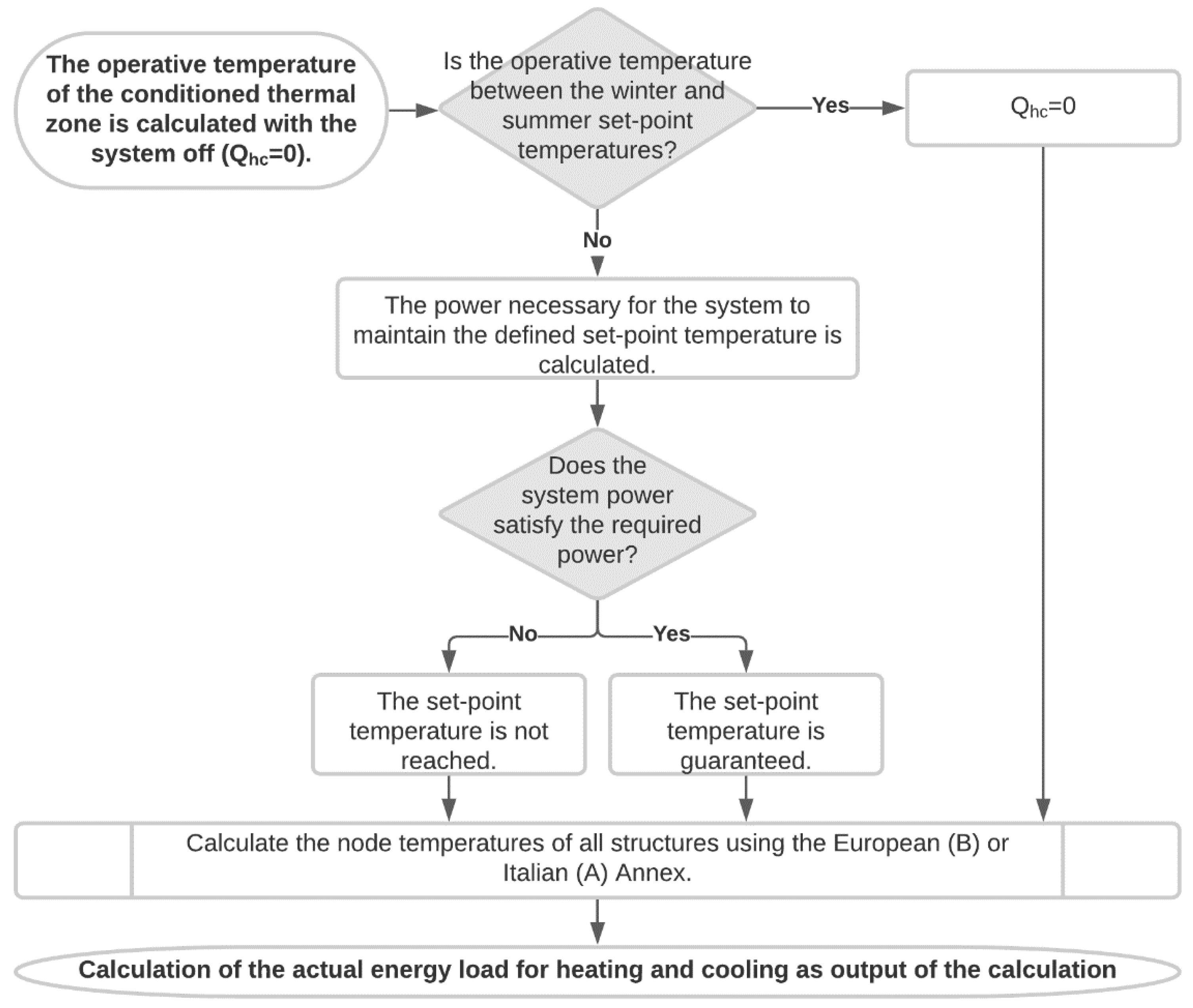
2.1. EN ISO 52016-1:2017
- in absence of heating and cooling plant the internal operating temperature is evaluated; if this is between the heating and cooling set-point temperature, the system is not switched on and the output power is zero;
- if the operating temperature is lower/upper than the heating/cooling set-point respectively, the power required by the system to guarantee the defined set-point temperature is calculated;
- if the power of the system is sufficient, the set-point temperature is guaranteed;
- if the power of the system is not sufficient, the set-point temperature is not reached;
- the node temperatures of all the structures are determined according to the European or National Annex;
- the effective energy load for heating and cooling is determined.
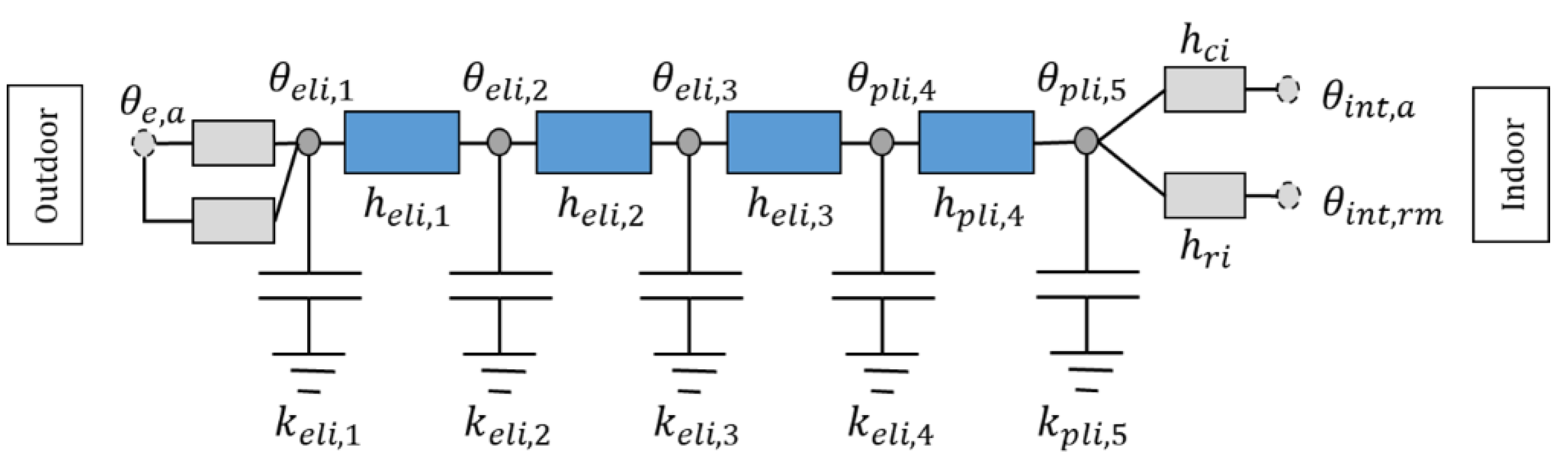
- the balance of the inside-facing node that considers the convective heat exchanges with the inside air, the conductive heat exchanges with the first node inside the opaque element, the heat exchanges by radiation with the surface nodes of all the structures delimiting the thermal zone, the eventual heat capacity associated with the surface node considered and the complementary quotas of the convective fractions of the total internal contributions, the solar contributions transmitted through the glass surfaces and the contributions due to the load of the heating/cooling system.
- the energy balances of the nodes inside the opaque element that consider the conductive thermal exchanges with adjacent nodes and any associated thermal capacities of the nodes.
- the balance of the outside-facing node, which considers convective heat exchanges with the outside air, radiation heat exchanges with the sky and solar contributions calculated as a function of the solar absorption coefficient, direct and diffuse solar radiation and any shading factor due to external obstacles.
2.1.1. European Annex
2.1.2. Italian Annex
- ρj: density of the material of the j-th layer of the building element (kg/m3)
- cj: thermal capacity of the j-th layer of the building element (J/(kg∙K))
- dj: thickness of the j-th layer of the building element (m)
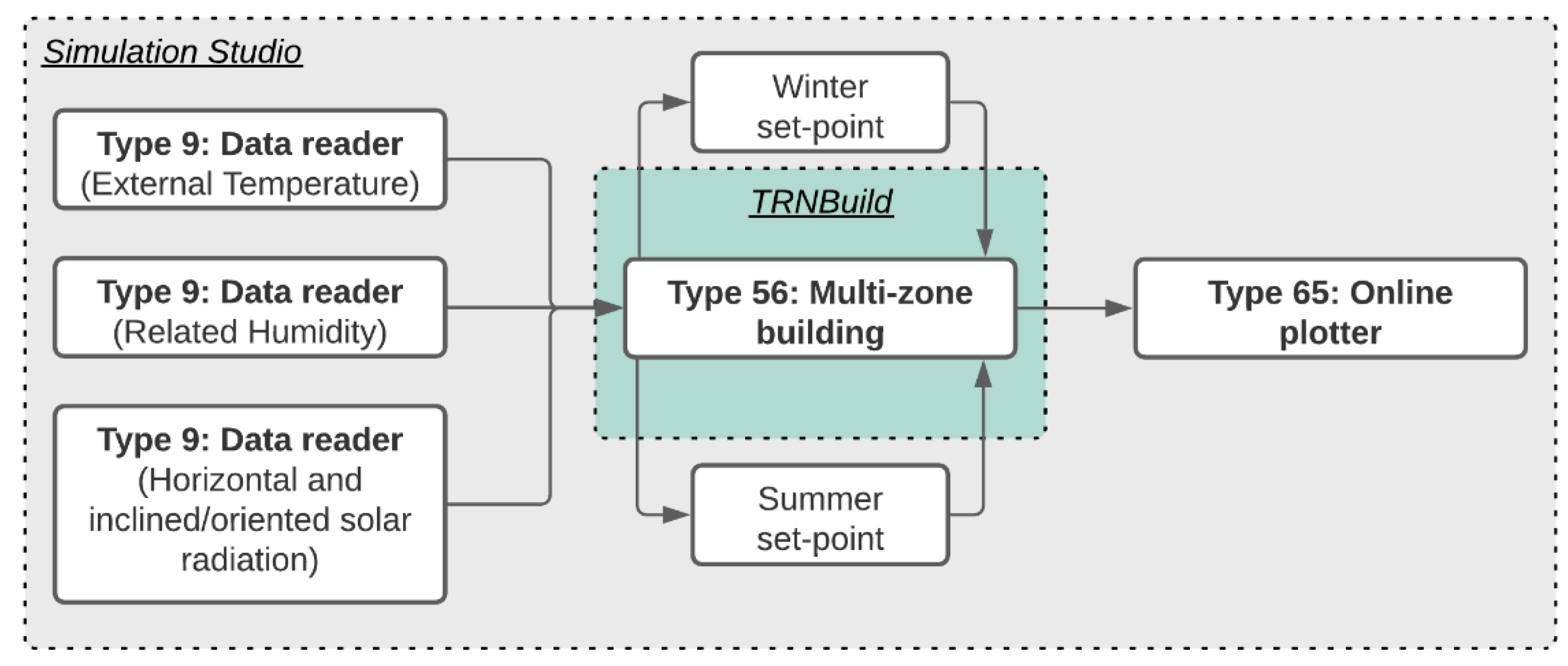
2.2. Trnsys
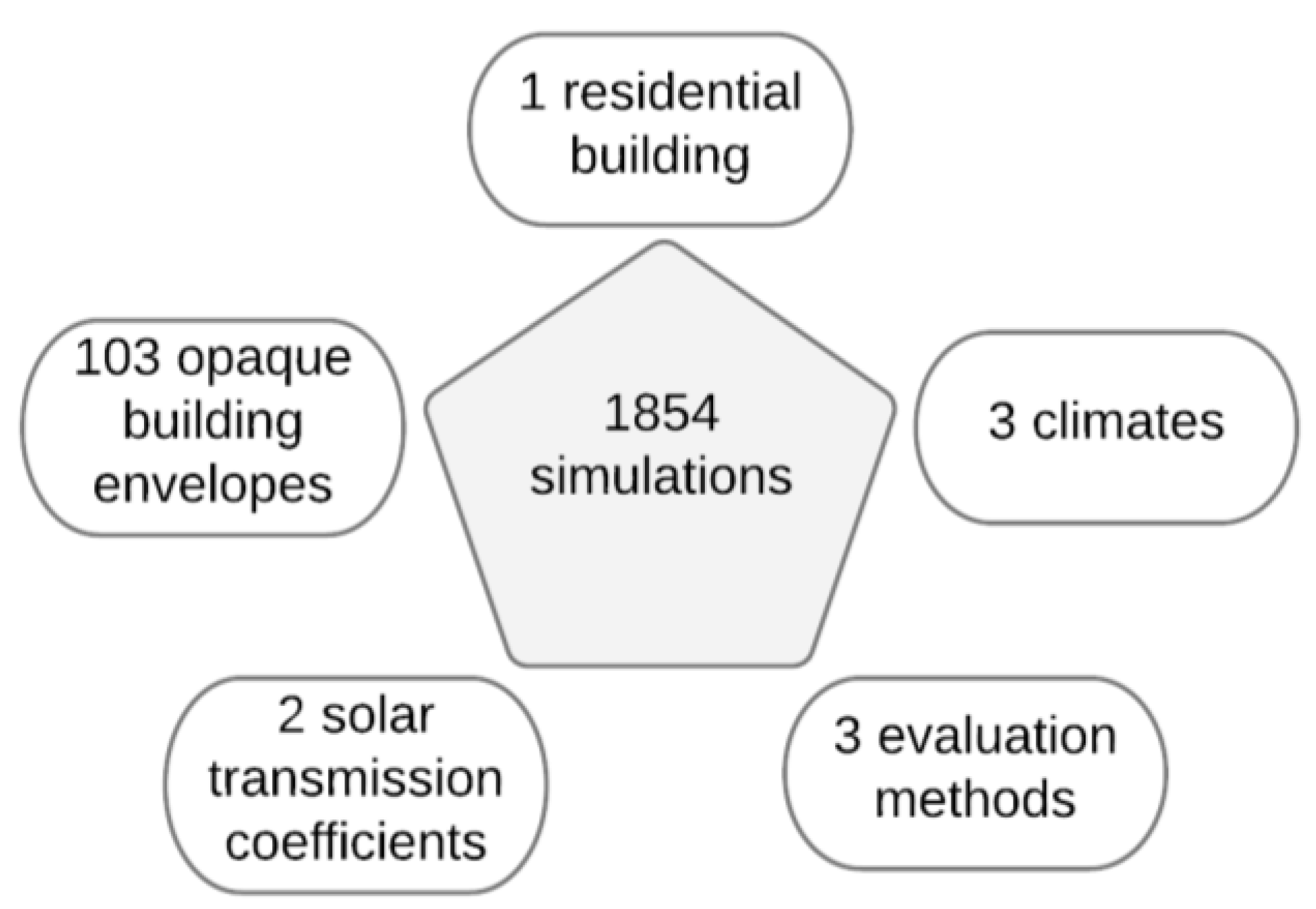
3. Case Studies
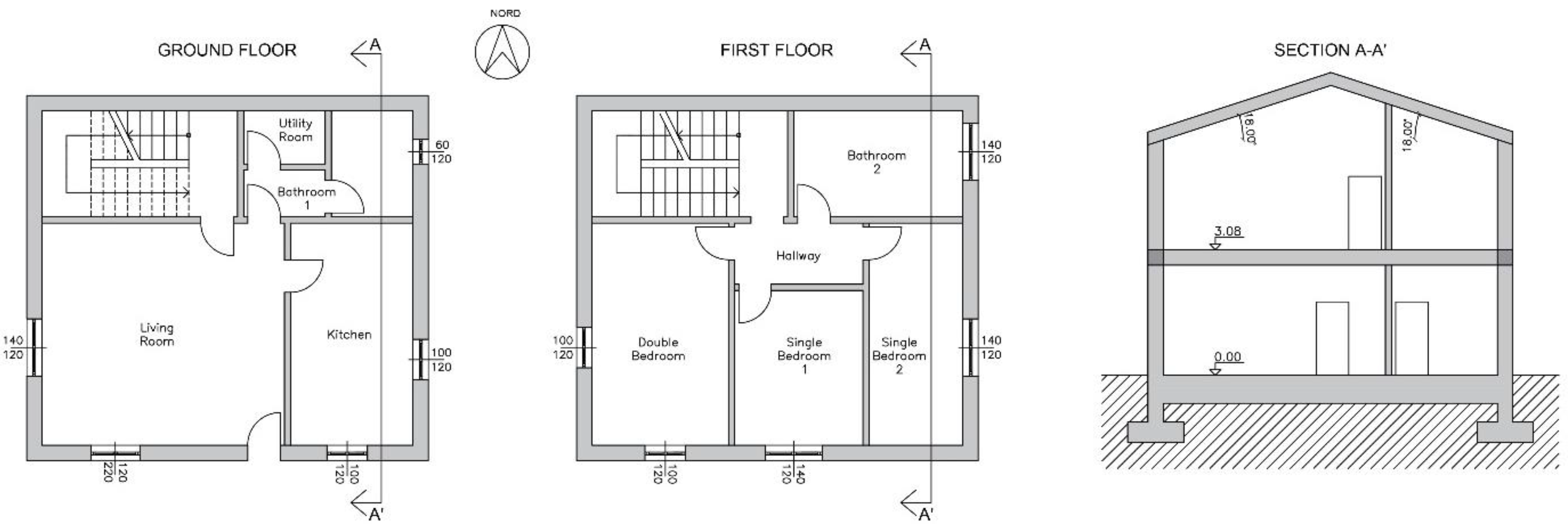
3.1. Geometry and Zoning
3.2. Opaque Surfaces
3.3. Transparent Surfaces
3.4. Climate and Other Assumptions
4. Results and Discussion
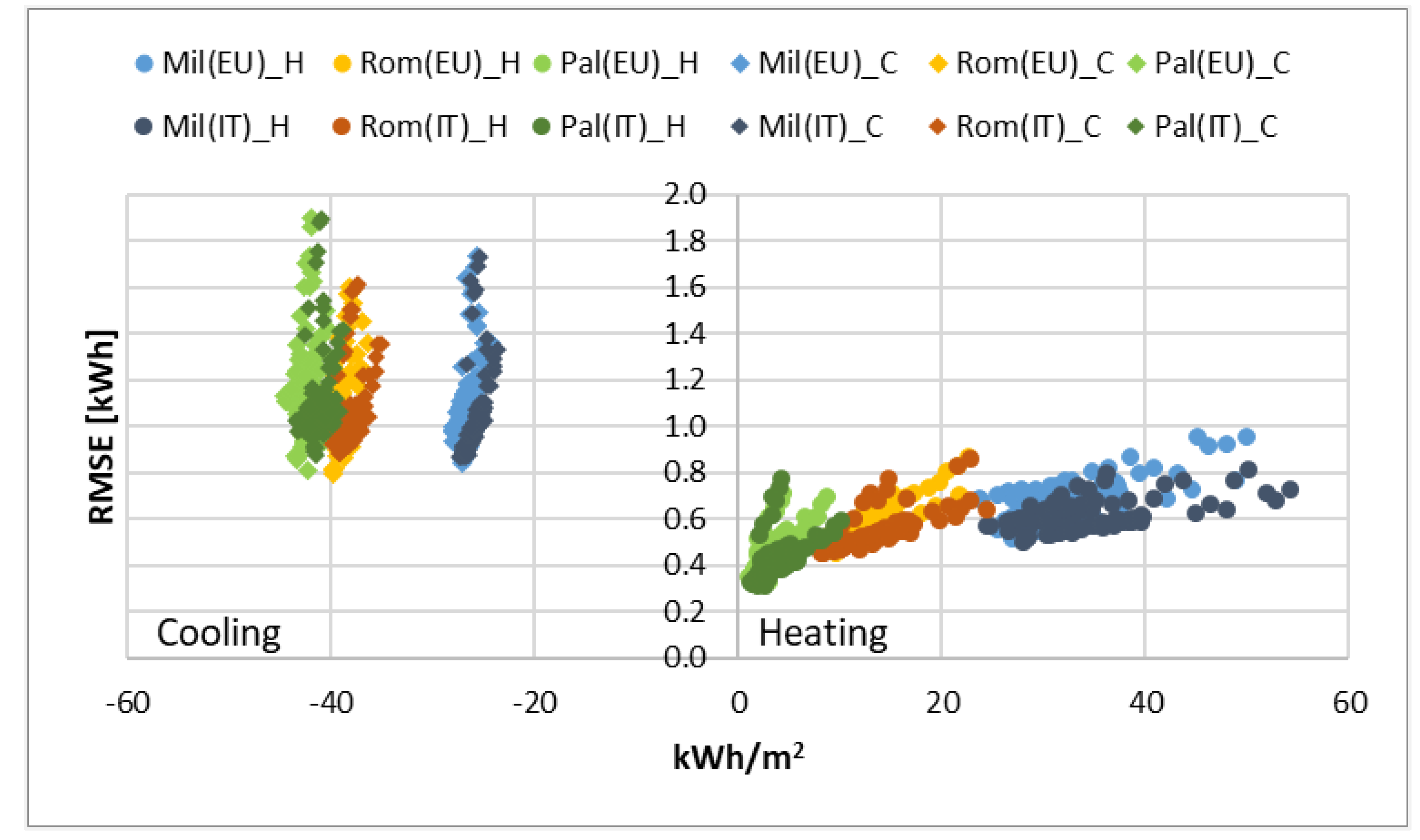
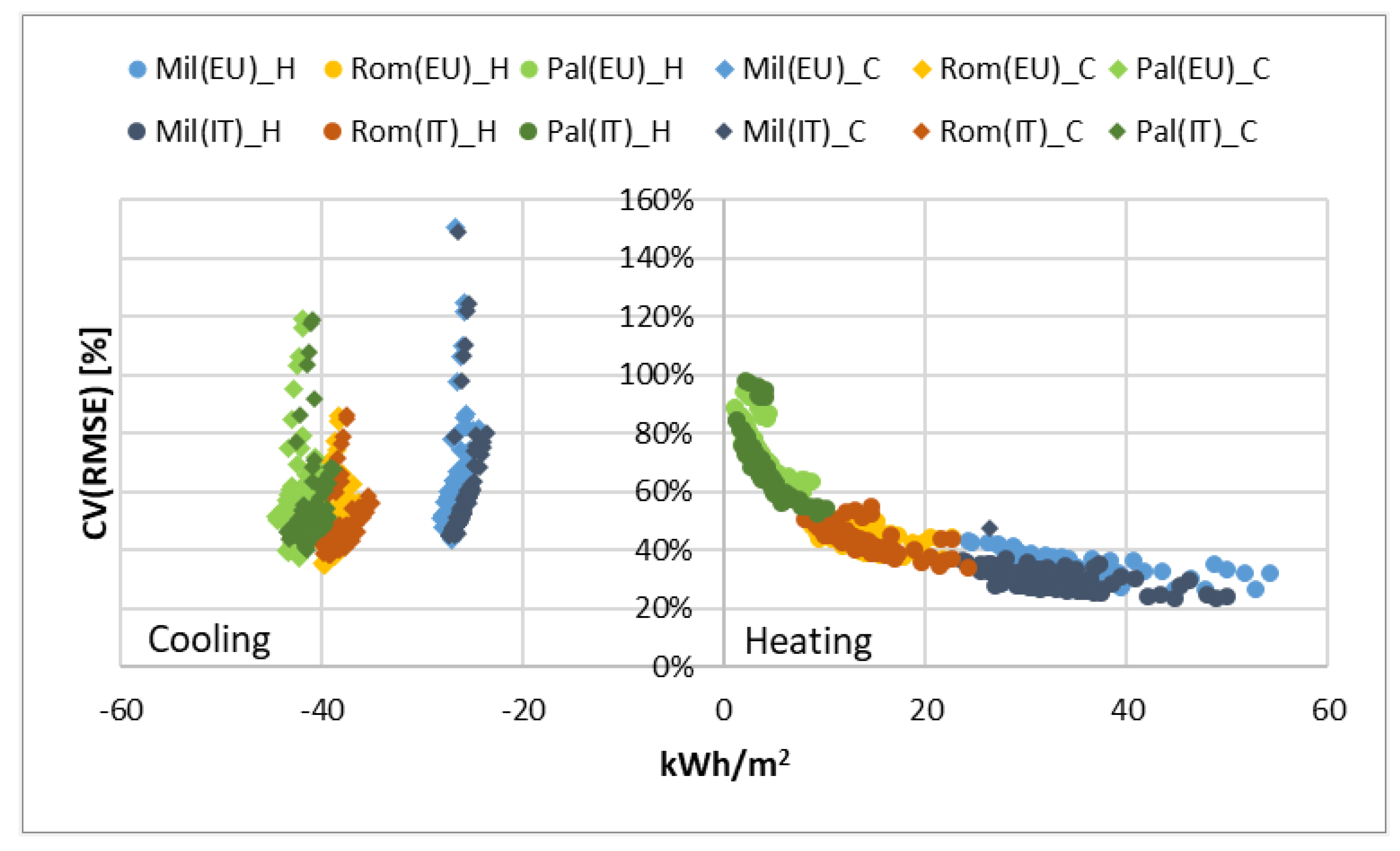
4.1. Accuracy of the Standard (European and Italian Annex)
4.2. Impact of the Solar Transmission Coefficient (ggl) on the Calculation of Energy Needs
Improved Calculation of the Total Solar Energy Transmission Coefficient (ggl)
4.3. Sensitivity Analysis of the Thermophysical Parameters of Opaque Walls on the Calculation of Energy Needs
5. Conclusions
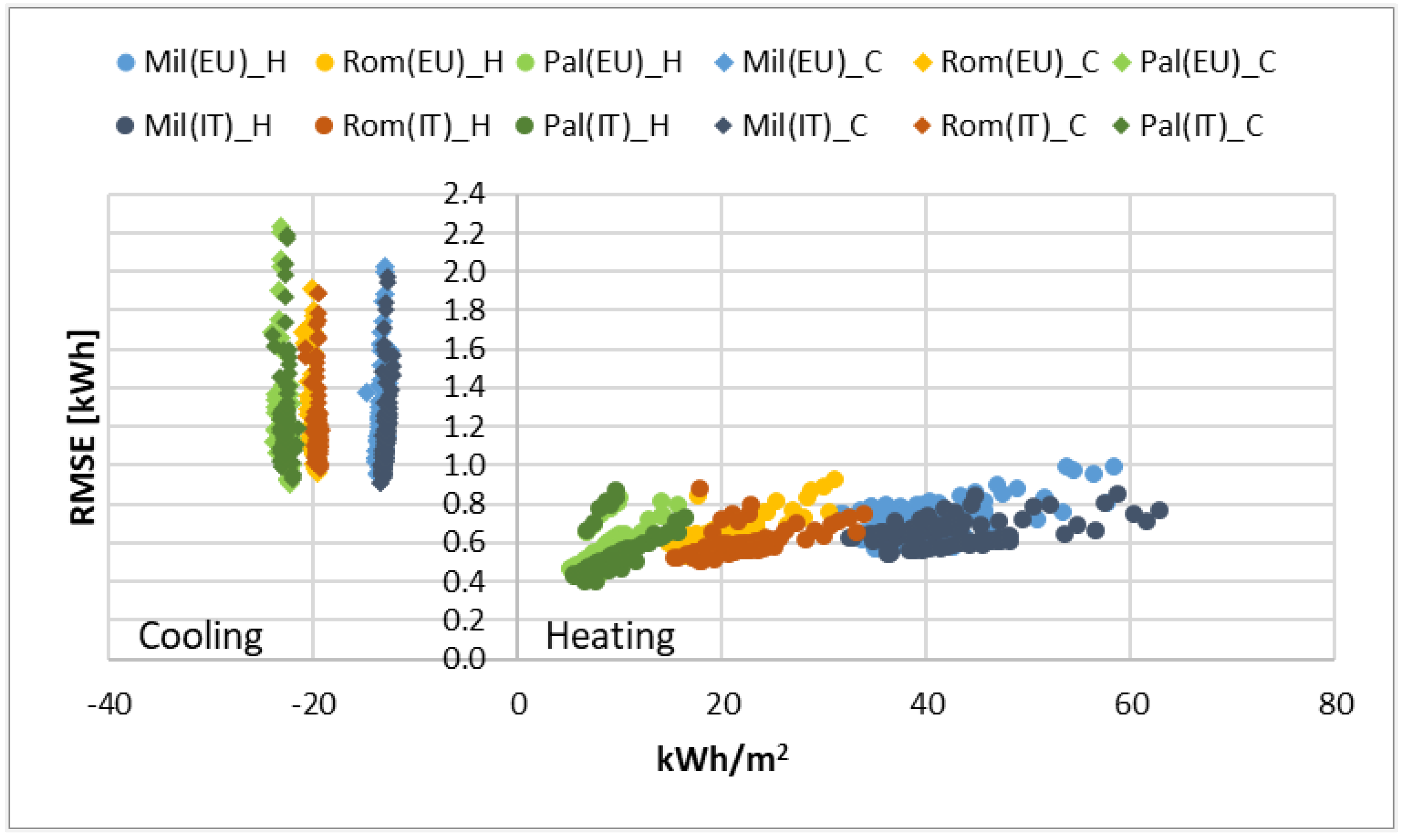
- The absolute error RMSE is extremely small. Both methods show variations of less than 1 kWh for heating, while for cooling the variations are less than 2 kWh (in the case of ggl,n = 0.77) and less than 2.2 kWh (in the case of ggl,n = 0.34). In absolute terms, Annex A performs better. This result is congruent with the comparative analysis carried out by Mazzarella et al. [12] between the two models of the Annexes and the analytical solution with sinusoidal boundary conditions. In all the test cases, the results obtained applying the Italian Annex provide better results, with a reduction of the error on the internal flow amplitude between 14% and 67% and an overestimation of the external flow amplitude compared to the analytical solution of 3%.
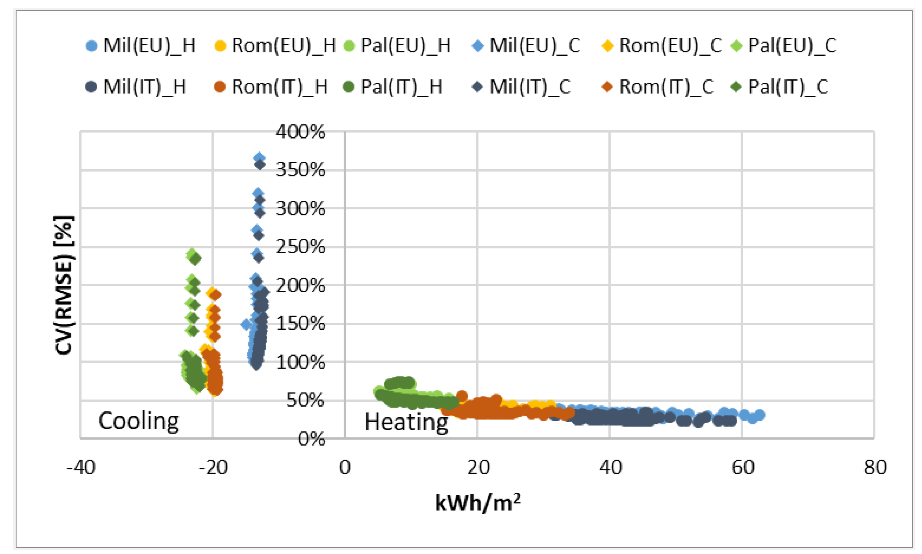
- The relative error CV(RMSE) is often over the 30% ASHRAE limit. It should be noted, however, that this is mainly caused by the low energy requirements of the analyzed solutions, which affect the denominator of the relative error formula. Only in the winter phase and for the coldest city the CV(RMSE) is verified. Specifically, for the case study with ggl,n = 0.77 the verification is satisfied for 16 cases (5.2%) with Annex B and for 45 cases (14.6%) with Annex A, while for the case study with ggl,n = 0.34, 51 cases (16.5%) with Annex B and 81 cases (26.2%) with Annex A. The contrast between the excellent results obtained in terms of RMSE and the low percentage of cases that satisfy the limit of 30% in terms of CV (RMSE) leads us to affirm that the verification proposed by ASHRAE to validate dynamic calculation methods, is not fully adequate in the case of low-energy buildings.
- In general, decreasing the ggl (thus increasing the performance of the glazed structures) produces a higher RMSE. Indeed, a worse average error of 12.9% and 11.6% is obtained in the winter season for the method described in Annex B and Annex A, respectively, while 9.3% and 11.7% in the summer season. These results suggest that the EN ISO 52016-1 algorithm, regardless of the annex used, has an accuracy inversely proportional to the performance of the building: the lower the consumption, the greater the error committed with respect to the energy needs calculated by Trnsys.
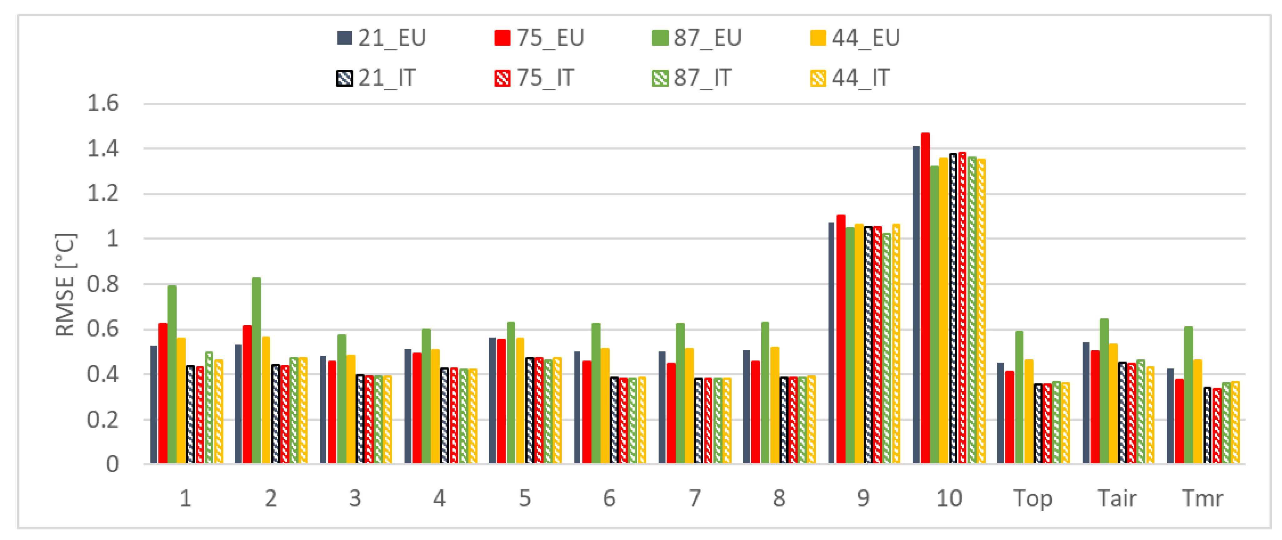
- In terms of internal and surface temperatures, the RMSE of Annex B compared to Trnsys seems to vary according to the positioning of the mass inside the wall, with the worst result for the wall with external mass. For Annex A, the RMSE is approximately constant for each proposed solution. This allows us to state that the heat transfer model of the opaque elements proposed in the European Annex (Annex B) favors some masonry types over others, in particular the one with distributed thermal mass. Overestimating the surface temperatures of the thermal zones implies an incorrect calculation of the operating temperature and consequently an incorrect energy requirement.
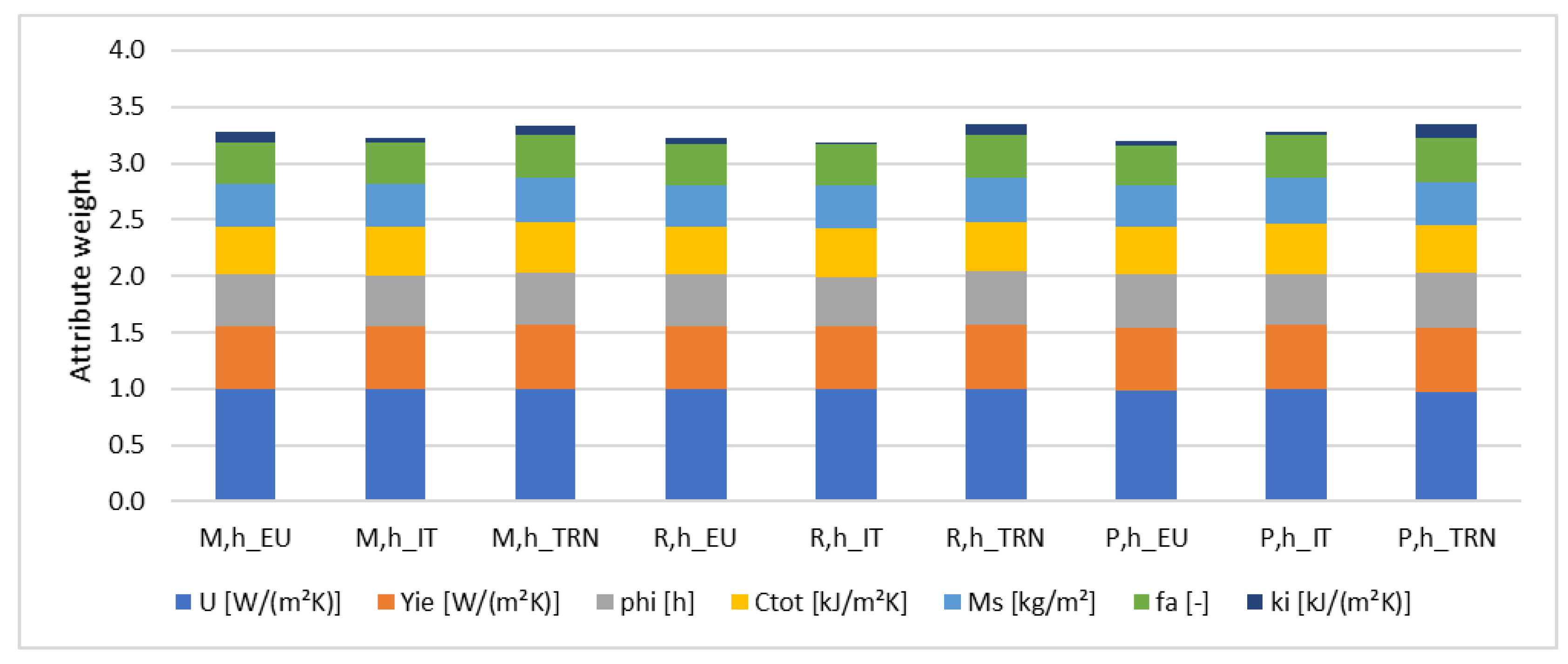
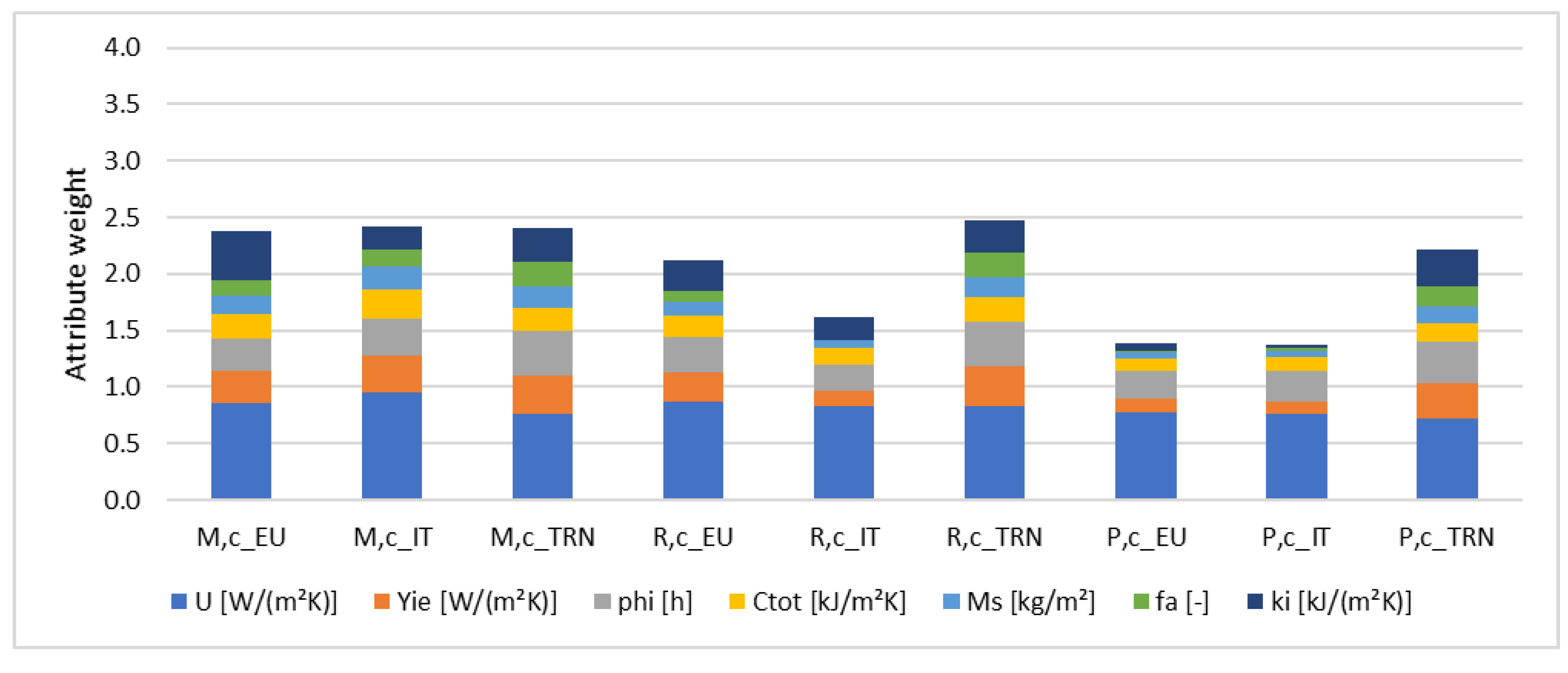
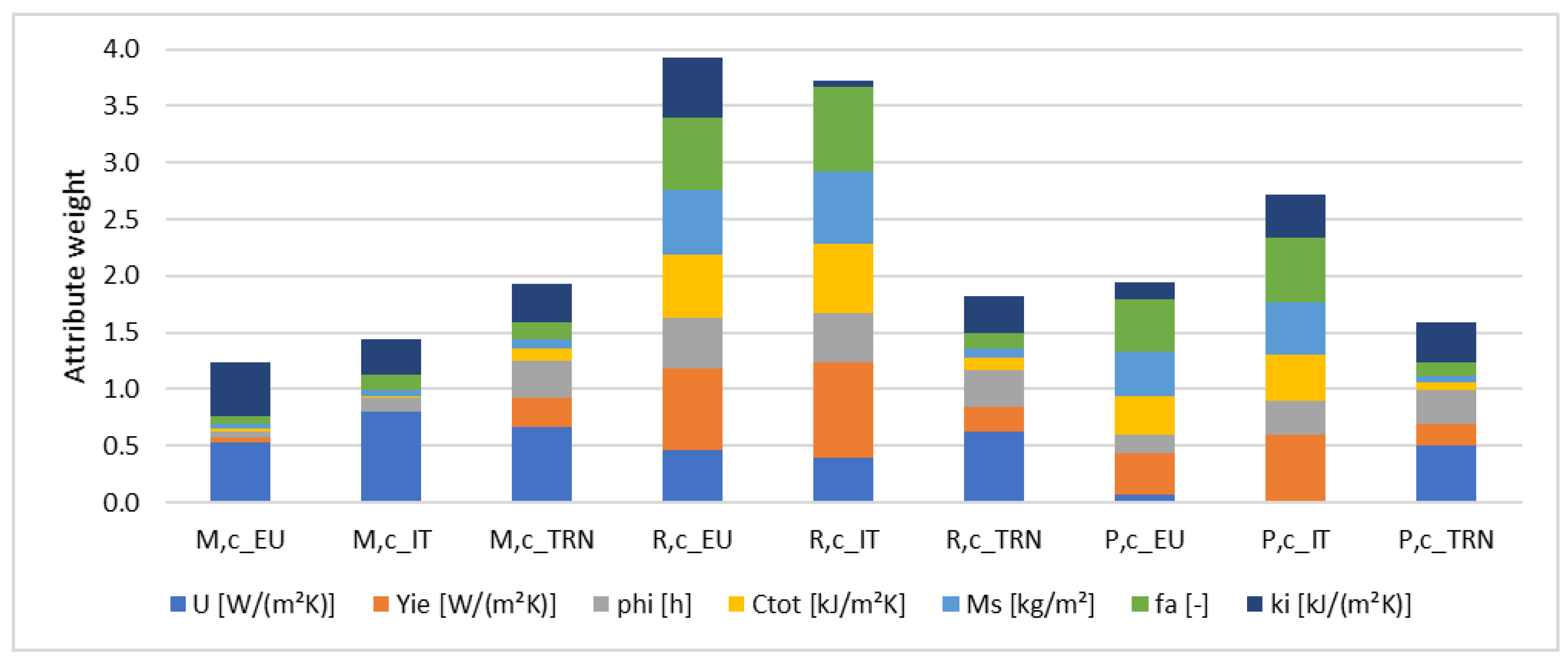
- Through a sensitivity analysis of the thermo-physical parameters of the walls, it can be stated that in the heating period the different calculation models are particularly aligned. In the summer period, on the other hand, the weights of the contributions are very variable for the different methods and the different case studies. In particular, for solar transmission coefficient equal to 0.34, the weights of the attributes calculated by Annex A and Annex B seem to have no correspondence with the weights calculated by Trnsys.
- Although ISO 52016-1 considers the angle of incidence of solar radiation, it overlooks that ggl can vary considerably depending on the time of day and the day of the year. Implementing the Karlsson et al. method [16] within the general algorithm allows to improve the RMSE of summer solar loads by 46.7% compared to the method proposed by the standard. Improving the estimation of solar loads allows an improvement in the calculation of summer needs.
References
Author Contributions
Funding
Conflicts of Interest
Abbreviations
| U | Thermal transmittance | W/(m2K) |
| Ms | Surface mass | kg/m2 |
| YIE | Periodic thermal transmittance | W/(m2K) |
| fa | Attenuation factor | - |
| φ/phi | Phase shift | h |
| κj | Internal areal heat capacity | kJ/(m2K) |
| Ctot | Total heat capacity | kJ/(m2K) |
| ggl | Total solar energy trasmittance | - |
| ggl,n | Total normal transmittance of solar energy | - |
| Fw | Exposition factor | - |
| Isol,dir/dif,t | Direct/diffuse solar radiation incident on the glazed surface | W/m2 |
| Fsh,obst,t | Shading reduction factor | - |
| ϑsol,t | Angle of incidence of direct solar radiation | ° |
| p | Number of glass panels | - |
| q | Coefficient of glass coating type | - |
| θe | Outdoor temperature | °C |
| IH | Horizontal solar radiation | W/m2 |
| HDD | Heating degree days | - |
Appendix A. Specifications of the Opaque Structures Used

| N. | Distribution of Mass | U | Ms | YIE | fa | φ | κj |
|---|---|---|---|---|---|---|---|
| - | - | W/(m2K) | kg/m2 | W/(m2K) | - | h | kJ/(m2K) |
| 1 | D | 0.228 | 315.00 | 0.004 | 0.019 | 23.10 | 44.12 |
| 2 | D | 0.315 | 246.00 | 0.019 | 0.060 | 18.75 | 37.60 |
| 3 | D | 0.343 | 294.00 | 0.018 | 0.052 | 18.18 | 44.02 |
| 4 | D | 0.230 | 432.00 | 0.001 | 0.005 | 5.93 | 39.57 |
| 5 | D | 0.355 | 228.00 | 0.026 | 0.074 | 16.83 | 39.10 |
| 6 | D | 0.368 | 353.20 | 0.013 | 0.036 | 20.83 | 41.74 |
| 7 | D | 0.356 | 274.85 | 0.018 | 0.050 | 18.55 | 40.55 |
| 8 | D | 0.237 | 228.86 | 0.007 | 0.031 | 21.10 | 35.77 |
| 9 | D | 0.218 | 227.80 | 0.007 | 0.031 | 21.92 | 34.56 |
| 10 | D | 0.163 | 292.99 | 0.001 | 0.006 | 29.22 | 34.36 |
| 11 | D | 0.238 | 265.09 | 0.006 | 0.026 | 22.70 | 36.17 |
| 12 | D | 0.243 | 444.15 | 0.002 | 0.010 | 26.95 | 38.85 |
| 13 | D | 0.208 | 444.15 | 0.001 | 0.004 | 29.08 | 38.86 |
| 14 | D | 0.343 | 375.06 | 0.011 | 0.033 | 20.35 | 41.30 |
| 15 | D | 0.209 | 360.00 | 0.001 | 0.005 | 28.72 | 41.93 |
| 16 | D | 0.215 | 287.00 | 0.003 | 0.015 | 25.35 | 39.77 |
| 17 | D | 0.169 | 369.00 | 0.001 | 0.003 | 32.77 | 39.80 |
| 18 | D | 0.192 | 328.00 | 0.001 | 0.007 | 28.88 | 39.87 |
| 19 | D | 0.239 | 308.25 | 0.004 | 0.017 | 24.57 | 37.29 |
| 20 | D | 0.310 | 404.10 | 0.005 | 0.016 | 24.70 | 41.48 |
| 21 | D | 0.230 | 432.00 | 0.001 | 0.005 | 5.93 | 39.57 |
| 22 | D | 0.215 | 52.13 | 0.120 | 0.554 | 6.67 | 21.63 |
| 23 | D | 0.244 | 49.63 | 0.154 | 0.631 | 5.87 | 22.12 |
| 24 | D | 0.364 | 44.18 | 0.288 | 0.793 | 4.31 | 22.79 |
| 25 | D | 0.281 | 47.93 | 0.191 | 0.679 | 5.50 | 22.24 |
| 26 | D | 0.383 | 43.55 | 0.310 | 0.810 | 4.13 | 22.66 |
| 27 | D | 0.292 | 47.30 | 0.204 | 0.699 | 5.30 | 22.38 |
| 28 | D | 0.271 | 48.55 | 0.179 | 0.660 | 5.70 | 22.22 |
| 29 | D | 0.371 | 199.50 | 0.048 | 0.130 | 13.80 | 44.38 |
| 30 | D | 0.296 | 265.60 | 0.013 | 0.044 | 20.20 | 37.73 |
| 31 | D | 0.285 | 345.60 | 0.006 | 0.020 | 23.76 | 39.50 |
| 32 | D | 0.262 | 187.60 | 0.020 | 0.075 | 17.86 | 34.47 |
| 33 | D | 0.380 | 246.75 | 0.040 | 0.105 | 15.40 | 38.84 |
| 34 | D | 0.275 | 270.00 | 0.007 | 0.027 | 21.40 | 41.82 |
| 35 | D | 0.352 | 180.00 | 0.036 | 0.102 | 15.08 | 41.94 |
| 36 | D | 0.363 | 164.00 | 0.059 | 0.163 | 14.21 | 39.97 |
| 37 | D | 0.252 | 246.00 | 0.009 | 0.035 | 21.50 | 39.74 |
| 38 | D | 0.402 | 196.00 | 0.059 | 0.146 | 13.08 | 44.58 |
| 39 | D | 0.518 | 246.75 | 0.090 | 0.173 | 12.90 | 42.23 |
| 40 | D | 0.482 | 41.05 | 0.422 | 0.875 | 3.20 | 22.12 |
| 41 | IE | 0.323 | 286.44 | 0.135 | 0.418 | 6.73 | 50.13 |
| 42 | IE | 0.233 | 278.64 | 0.056 | 0.241 | 10.70 | 42.74 |
| 43 | IE | 0.369 | 271.14 | 0.115 | 0.310 | 8.68 | 43.64 |
| 44 | IE | 0.226 | 20.55 | 0.192 | 0.888 | 3.81 | 34.26 |
| 45 | IE | 0.248 | 19.95 | 0.223 | 0.901 | 3.46 | 33.99 |
| 46 | IE | 0.350 | 18.75 | 0.321 | 0.918 | 2.88 | 33.20 |
| 47 | IE | 0.339 | 272.38 | 0.048 | 0.141 | 14.28 | 42.76 |
| 48 | IE | 0.266 | 276.13 | 0.033 | 0.125 | 15.30 | 42.52 |
| 49 | IE | 0.376 | 285.19 | 0.067 | 0.178 | 12.41 | 49.46 |
| 50 | IE | 0.295 | 285.94 | 0.050 | 0.169 | 12.80 | 49.37 |
| 51 | IE | 0.260 | 25.10 | 0.227 | 0.871 | 3.96 | 36.96 |
| 52 | IE | 0.303 | 19.20 | 0.276 | 0.913 | 3.08 | 33.53 |
| 53 | IE | 0.322 | 24.35 | 0.284 | 0.883 | 3.58 | 36.54 |
| 54 | IE | 0.368 | 18.60 | 0.339 | 0.920 | 2.83 | 33.08 |
| 55 | IE | 0.598 | 17.55 | 0.570 | 0.953 | 2.03 | 26.22 |
| 56 | IE | 0.561 | 14.98 | 0.528 | 0.941 | 2.22 | 30.39 |
| 57 | I | 0.259 | 249.13 | 0.008 | 0.031 | 20.56 | 37.70 |
| 58 | I | 0.269 | 248.50 | 0.009 | 0.034 | 20.36 | 37.69 |
| 59 | I | 0.253 | 229.50 | 0.010 | 0.041 | 17.90 | 39.16 |
| 60 | I | 0.298 | 228.90 | 0.015 | 0.051 | 17.50 | 39.13 |
| 61 | I | 0.326 | 228.60 | 0.020 | 0.061 | 17.20 | 39.11 |
| 62 | I | 0.278 | 354.10 | 0.004 | 0.015 | 22.81 | 41.87 |
| 63 | I | 0.317 | 353.65 | 0.006 | 0.020 | 22.33 | 41.83 |
| 64 | I | 0.255 | 381.31 | 0.004 | 0.016 | 21.68 | 41.89 |
| 65 | I | 0.264 | 380.69 | 0.005 | 0.018 | 21.53 | 41.39 |
| 66 | I | 0.284 | 379.44 | 0.006 | 0.021 | 21.25 | 41.37 |
| 67 | I | 0.287 | 238.60 | 0.035 | 0.121 | 12.30 | 45.99 |
| 68 | I | 0.328 | 238.15 | 0.042 | 0.128 | 12.10 | 46.10 |
| 69 | I | 0.383 | 237.70 | 0.053 | 0.138 | 11.90 | 46.25 |
| 70 | I | 0.262 | 404.70 | 0.002 | 0.007 | 2.36 | 41.51 |
| 71 | I | 0.208 | 253.50 | 0.004 | 0.020 | 21.68 | 37.76 |
| 72 | I | 0.207 | 230.40 | 0.007 | 0.033 | 18.35 | 39.18 |
| 73 | I | 0.197 | 355.60 | 0.002 | 0.009 | 23.60 | 41.90 |
| 74 | I | 0.211 | 385.06 | 0.003 | 0.014 | 22.55 | 41.41 |
| 75 | I | 0.227 | 405.30 | 0.001 | 0.005 | 26.85 | 41.52 |
| 76 | I | 0.214 | 239.80 | 0.023 | 0.109 | 12.88 | 45.83 |
| 77 | I | 0.345 | 238.00 | 0.045 | 0.131 | 12.03 | 46.14 |
| 78 | I | 0.580 | 236.80 | 0.109 | 0.187 | 11.32 | 47.08 |
| 79 | I | 0.462 | 237.25 | 0.071 | 0.154 | 11.67 | 46.52 |
| 80 | I | 0.505 | 196.25 | 0.121 | 0.239 | 9.67 | 47.52 |
| 81 | E | 0.208 | 253.50 | 0.005 | 0.022 | 21.45 | 23.47 |
| 82 | E | 0.207 | 230.40 | 0.008 | 0.039 | 18.03 | 21.56 |
| 83 | E | 0.197 | 355.60 | 0.002 | 0.011 | 23.26 | 21.57 |
| 84 | E | 0.211 | 385.06 | 0.003 | 0.016 | 22.26 | 23.58 |
| 85 | E | 0.214 | 239.80 | 0.030 | 0.139 | 12.51 | 21.94 |
| 86 | E | 0.345 | 238.00 | 0.056 | 0.163 | 11.65 | 22.01 |
| 87 | E | 0.227 | 405.30 | 0.001 | 0.006 | 2.53 | 22.33 |
| 88 | E | 0.259 | 249.13 | 0.009 | 0.033 | 20.33 | 25.14 |
| 89 | E | 0.269 | 248.50 | 0.010 | 0.036 | 20.13 | 26.10 |
| 90 | E | 0.274 | 229.20 | 0.014 | 0.052 | 17.40 | 22.27 |
| 91 | E | 0.298 | 228.90 | 0.017 | 0.058 | 17.18 | 23.17 |
| 92 | E | 0.278 | 354.10 | 0.005 | 0.017 | 22.46 | 23.19 |
| 93 | E | 0.317 | 353.65 | 0.007 | 0.022 | 22.00 | 26.93 |
| 94 | E | 0.255 | 381.31 | 0.005 | 0.020 | 21.36 | 23.31 |
| 95 | E | 0.264 | 380.69 | 0.006 | 0.022 | 21.21 | 23.40 |
| 96 | E | 0.284 | 379.44 | 0.007 | 0.024 | 20.93 | 23.87 |
| 97 | E | 0.321 | 377.56 | 0.010 | 0.031 | 20.41 | 26.16 |
| 98 | E | 0.328 | 238.15 | 0.052 | 0.159 | 11.71 | 21.91 |
| 99 | E | 0.383 | 237.70 | 0.065 | 0.170 | 11.50 | 22.33 |
| 100 | E | 0.262 | 404.70 | 0.002 | 0.008 | 2.05 | 25.21 |
| 101 | E | 0.538 | 199.28 | 0.135 | 0.251 | 10.77 | 29.74 |
| 102 | E | 0.442 | 201.15 | 0.090 | 0.205 | 11.35 | 25.41 |
| 103 | E | 0.417 | 201.78 | 0.081 | 0.195 | 11.50 | 24.77 |
Appendix B. Sensitivity Analysis of Thermo-Physical Parameters of Opaque Structures
| Range | Upper limit |
| 0.000–0.150 | 0.150 |
| 0.151–0.300 | 0.150 |
| 0.301–0.450 | 0.450 |
| 0.451–0.600 | 0.600 |
| 0.601–0.750 | 0.600 |
| 0.751–0.900 | 0.900 |
| 0.901–1.000 | 1.000 |
| M,h_EU | M,h_IT | M,h_TRN | R,h_EU | R,h_IT | R,h_TRN | P,h_EU | P,h_IT | P,h_TRN | |
|---|---|---|---|---|---|---|---|---|---|
| U [W/(m2K)] | 0.999 | 0.996 | 0.997 | 0.998 | 0.992 | 0.994 | 0.979 | 0.985 | 0.974 |
| Yie [W/(m2K)] | 0.564 | 0.567 | 0.576 | 0.565 | 0.526 | 0.580 | 0.585 | 0.604 | 0.592 |
| phi [h] | 0.468 | 0.454 | 0.479 | 0.470 | 0.444 | 0.484 | 0.477 | 0.479 | 0.500 |
| Ctot [kJ/m2K] | 0.439 | 0.448 | 0.453 | 0.437 | 0.430 | 0.452 | 0.457 | 0.479 | 0.451 |
| Ms [kg/m2] | 0.388 | 0.396 | 0.405 | 0.385 | 0.374 | 0.405 | 0.403 | 0.426 | 0.408 |
| fa [-] | 0.378 | 0.376 | 0.392 | 0.376 | 0.347 | 0.396 | 0.395 | 0.409 | 0.414 |
| ki [kJ/(m2K)] | 0.053 | 0.030 | 0.077 | 0.028 | 0.038 | 0.082 | 0.099 | 0.041 | 0.102 |
| M,c_EU | M,c_IT | M,c_TRN | R,c_EU | R,c_IT | R,c_TRN | P,c_EU | P,c_IT | P,c_TRN | |
|---|---|---|---|---|---|---|---|---|---|
| U [W/(m2K)] | 0.852 | 0.954 | 0.762 | 0.876 | 0.833 | 0.825 | 0.775 | 0.759 | 0.727 |
| Yie [W/(m2K)] | 0.291 | 0.322 | 0.345 | 0.253 | 0.127 | 0.352 | 0.123 | 0.116 | 0.303 |
| phi [h] | 0.290 | 0.325 | 0.385 | 0.310 | 0.243 | 0.394 | 0.244 | 0.273 | 0.365 |
| Ctot [kJ/m2K] | 0.208 | 0.259 | 0.211 | 0.190 | 0.138 | 0.220 | 0.113 | 0.121 | 0.170 |
| Ms [kg/m2] | 0.163 | 0.200 | 0.184 | 0.129 | 0.072 | 0.186 | 0.043 | 0.055 | 0.143 |
| fa [-] | 0.135 | 0.151 | 0.221 | 0.088 | 0.001 | 0.214 | 0.025 | 0.028 | 0.186 |
| ki [kJ/(m2K)] | 0.439 | 0.203 | 0.302 | 0.273 | 0.206 | 0.288 | 0.061 | 0.022 | 0.320 |
| M,h_EU | M,h_IT | M,h_TRN | R,h_EU | R,h_IT | R,h_TRN | P,h_EU | P,h_IT | P,h_TRN | |
|---|---|---|---|---|---|---|---|---|---|
| U [W/(m2K)] | 0.998 | 0.996 | 0.996 | 0.999 | 0.995 | 0.993 | 0.988 | 0.993 | 0.970 |
| Yie [W/(m2K)] | 0.552 | 0.556 | 0.566 | 0.551 | 0.553 | 0.568 | 0.556 | 0.572 | 0.566 |
| phi [h] | 0.463 | 0.447 | 0.473 | 0.459 | 0.445 | 0.477 | 0.467 | 0.454 | 0.488 |
| Ctot [kJ/m2K] | 0.428 | 0.438 | 0.442 | 0.424 | 0.433 | 0.439 | 0.423 | 0.452 | 0.425 |
| Ms [kg/m2] | 0.378 | 0.386 | 0.393 | 0.372 | 0.380 | 0.392 | 0.368 | 0.398 | 0.382 |
| fa [-] | 0.365 | 0.365 | 0.381 | 0.361 | 0.358 | 0.383 | 0.358 | 0.378 | 0.389 |
| ki [kJ/(m2K)] | 0.092 | 0.042 | 0.085 | 0.061 | 0.025 | 0.095 | 0.033 | 0.037 | 0.129 |
| M,c_EU | M,c_IT | M,c_TRN | R,c_EU | R,c_IT | R,c_TRN | P,c_EU | P,c_IT | P,c_TRN | |
|---|---|---|---|---|---|---|---|---|---|
| U [W/(m2K)] | 0.537 | 0.798 | 0.670 | 0.461 | 0.394 | 0.619 | 0.064 | 0.014 | 0.510 |
| Yie [W/(m2K)] | 0.036 | 0.001 | 0.254 | 0.724 | 0.843 | 0.227 | 0.375 | 0.588 | 0.188 |
| phi [h] | 0.050 | 0.131 | 0.324 | 0.446 | 0.440 | 0.318 | 0.153 | 0.300 | 0.294 |
| Ctot [kJ/m2K] | 0.024 | 0.002 | 0.112 | 0.556 | 0.612 | 0.106 | 0.342 | 0.406 | 0.068 |
| Ms [kg/m2] | 0.050 | 0.063 | 0.082 | 0.565 | 0.630 | 0.083 | 0.394 | 0.455 | 0.054 |
| fa [-] | 0.063 | 0.136 | 0.145 | 0.642 | 0.753 | 0.135 | 0.461 | 0.579 | 0.119 |
| ki [kJ/(m2K)] | 0.481 | 0.312 | 0.341 | 0.531 | 0.055 | 0.334 | 0.149 | 0.376 | 0.357 |
References
- European Commission, A Roadmap for Moving to a Competitive Low Carbon Economy in 2050, European Commission. 2011. Available online: https://www.gazzettaufficiale.it/eli/gu/1993/10/14/242/so/96/sg/pdf (accessed on 1 November 2021).
- European Parliament, Energy. Topics: Energy Efficiency. Buildings, European Commission. 2018. Available online: https://eur-lex.europa.eu/legal-content/EN/TXT/PDF/?uri=CELEX:32018L0844&from=EN (accessed on 1 November 2021).
- European Parliament. Directive (EU) 2018/844 of the European Parliament and of the Council of 30 May 2018 amending Directive 2010/31/EU on the energy performance of buildings and Directive 2012/27/EU on energy efficiency. Off. J. Eur. Union. 2018, 75–91. [Google Scholar] [CrossRef]
- EN ISO 52016-1; 2017—Energy Performance of Buildings—Energy Needs for Heating and Cooling, Internal Temperatures and Sensible and Latent Head Loads—Part 1: Calculation Procedures Performance. International Organization for Standardization: Geneva, Switzerland, 2017.
- Zhang, H.; Shu, H. A Comprehensive Evaluation on Energy, Economic and Environmental Performance of the Trombe Wall during the Heating Season. J. Therm. Sci. 2019, 28, 1141–1149. [Google Scholar] [CrossRef]
- Bagarić, M.; Pečur, I.B.; Milovanović, B. Hygrothermal performance of ventilated prefabricated sandwich wall panel from recycled construction and demolition waste—A case study. Energy Build. 2020, 206, 109573. [Google Scholar] [CrossRef]
- Di Giuseppe, E.; Ulpiani, G.; Summa, S.; Tarabelli, L.; Di Perna, C.; D’Orazio, M. Hourly dynamic and monthly semi-stationary calculation methods applied to nZEBs: Impacts on energy and comfort. IOP Conf. Ser. Mater. Sci. Eng. 2019, 609, 072008. [Google Scholar] [CrossRef] [Green Version]
- Congedo, P.M.; Baglivo, C.; Centonze, G. Walls comparative evaluation for the thermal performance improvement of low-rise residential buildings in warm Mediterranean climate. J. Build. Eng. 2020, 28, 101059. [Google Scholar] [CrossRef]
- Ballarini, I.; Costantino, A.; Fabrizio, E.; Corrado, V. A Methodology to Investigate the Deviations between Simple and Detailed Dynamic Methods for the Building Energy Performance Assessment. Energies 2020, 13, 6217. [Google Scholar] [CrossRef]
- Zakula, T.; Bagaric, M.; Ferdelji, N.; Milovanovic, B.; Mudrinic, S.; Ritosa, K. Comparison of dynamic simulations and the ISO 52016 standard for the assessment of building energy performance. Appl. Energy 2019, 254, 113553. [Google Scholar] [CrossRef]
- Zakula, T.; Badun, N.; Ferdelji, N.; Ugrina, I. Framework for the ISO 52016 standard accuracy prediction based on the in-depth sensitivity analysis. Appl. Energy 2021, 298, 117089. [Google Scholar] [CrossRef]
- Mazzarella, L.; Scoccia, R.; Colombo, P.; Motta, M. Improvement to EN ISO 52016-1:2017 hourly heat transfer through a wall assessment: The Italian National Annex. Energy Build. 2020, 210, 109758. [Google Scholar] [CrossRef]
- Duffy, M.J.; Hiller, M.; Bradley, D.E.; Werner Keilholz, J.W. TRNSYS 17: A Transient System Simulation Program. 2013. Available online: https://sel.me.wisc.edu/trnsys/features/features.html (accessed on 1 November 2021).
- CEN European Commitee for Standardization. Indoor Environmental Input Parameters for Design and Assessment of Energy Performance of Buildings Addressing Indoor Air Quality, Thermal Environment, Lighting and Acoustics; EN 15251; CEN: Brussels, Belgium, 2007. [Google Scholar]
- Bergman, T.; Incropera, F.; DeWitt, D.; Lavine, A. Fundamentals of Heat and Mass Transfer, 7th ed.; Wiley: Hoboken, NJ, USA, 2011. [Google Scholar]
- Karlsson, J.; Roos, A. Modelling the angular behaviour of the total solar energy transmittance of windows. Sol. Energy 2000, 69, 321–329. [Google Scholar] [CrossRef]
- Shin, M.; Haberl, J.S. Thermal zoning for building HVAC design and energy simulation: A literature review. Energy Build. 2019, 203, 109429. [Google Scholar] [CrossRef]
- Minister of Economic Development, Italian Ministerial Decree of 5th July 1975: Modification to the ministerial instructions dated 20th June 1896 concerning the minimal height and the main hygienic-sanitary requirements in housing units, 1975 (1975) 18–20.
- UNI 10840; UNI-Ente Nazionale Italiano di Unificazione, 2007-Light and lighting-School rooms-General criteria for the artificial and natural lighting. UNI: Milan, Italy, 2007.
- Presidente Della Repubblica, Decreto del Presidente Della Repubblica 26 Agosto 1993, n. 412, Italy. 1993. Available online: https://www.gazzettaufficiale.it/eli/id/1993/10/14/093G0451/sg (accessed on 1 November 2021).
- ISO 52010-1:2017; International Organization for Standardization, Energy Performance of Buildings—External Climatic Conditions—Part 1: Conversion of Climatic Data for Energy Calculations. CEN: Brussels, Belgium, 2017.
- Summa, S.; Tarabelli, L.; Di Perna, C. Evaluation of ISO 52010-1:2017 and proposal for an alternative calculation procedure. Sol. Energy 2021, 218, 262–281. [Google Scholar] [CrossRef]
- Meteotest, Meteonorm 7 V7.3.3, Bern, Switzerland. 2018. Available online: https://meteonorm.com/en/ (accessed on 1 November 2021).
- Uni-Ente Nazionale Italiano Di Unificazione, Uni/Ts 11300-1:2014—Energy Performance of Buildings—Part 1: Evaluation of Energy Need for Space Heating and Cooling, Italy. 2014. Available online: http://store.uni.com/catalogo/norme/root-categorie-tc/uni/uni-ct-202/uni-ts-11300-1-2014?___store=en&___from_store=it (accessed on 1 November 2021).
- Recurve, Support Articles (FAQs), (n.d.). Available online: https://www.recurve.com/support-articles/what-is-a-cvrmse-value (accessed on 1 November 2021).
- ASHRAE Guideline 14, Measurement of Energy, Demand, and Water Savings. 2014. Available online: https://www.ashrae.org (accessed on 1 November 2021).
- Willmott, C.J.; Matsuura, K. On the use of dimensioned measures of error to evaluate the performance of spatial interpolators. Int. J. Geogr. Inf. Sci. 2006, 20, 89–102. [Google Scholar] [CrossRef]
- Moldovan, M.; Visa, I.; Neagoe, M.; Burduhos, B.G. Solar Heating & Cooling Energy Mixes to Transform Low Energy Buildings in Nearly Zero Energy Buildings. Energy Procedia 2014, 48, 924–937. [Google Scholar] [CrossRef] [Green Version]
- Yıldız, Y.; Arsan, Z.D. Identification of the building parameters that influence heating and cooling energy loads for apartment buildings in hot-humid climates. Energy 2011, 36, 4287–4296. [Google Scholar] [CrossRef] [Green Version]
- Li, H.; Wang, S.; Cheung, H. Sensitivity analysis of design parameters and optimal design for zero/low energy buildings in subtropical regions. Appl. Energy 2018, 228, 1280–1291. [Google Scholar] [CrossRef]
- Zhao, M.; Künzel, H.M.; Antretter, F. Parameters influencing the energy performance of residential buildings in different Chinese climate zones. Energy Build. 2015, 96, 64–75. [Google Scholar] [CrossRef]
- Mechri, H.E.; Capozzoli, A.; Corrado, V. USE of the ANOVA approach for sensitive building energy design. Appl. Energy 2010, 87, 3073–3083. [Google Scholar] [CrossRef]
- Rapidminer. Available online: https://rapidminer.com (accessed on 1 November 2021).

| Mass Position | κpl1,eli | κpl2,eli | κpl3,eli | κpl4,eli | κpl5,eli |
|---|---|---|---|---|---|
| I | 0 | 0 | 0 | 0 | κm,eli |
| E | κm,eli | 0 | 0 | 0 | 0 |
| IE | κm,eli/2 | 0 | 0 | 0 | κm,eli/2 |
| D | κm,eli/8 | κm,eli/4 | κm,eli/4 | κm,eli/4 | κm,eli/8 |
| M | 0 | 0 | κm,eli | 0 | 0 |
| Room | Afloor | V | havg | Awindow |
|---|---|---|---|---|
| - | m2 | m3 | m | m2 |
| Bathroom 1 | 7.50 | 20.25 | 2.70 | 0.41 |
| Utility Room | 2.60 | 7.02 | 2.70 | 0.00 |
| Kitchen | 16.35 | 44.15 | 2.70 | 1.64 |
| Living Room | 32.43 | 87.55 | 2.70 | 3.25 |
| Bathroom 2 | 10.79 | 33.69 | 3.12 | 1.22 |
| Hallway | 4.73 | 18.11 | 3.83 | 0.00 |
| Single Bedroom 1 | 11.97 | 39.71 | 3.32 | 1.22 |
| Single Bedroom 2 | 12.54 | 43.58 | 3.48 | 1.22 |
| Double Bedroom | 18.26 | 63.47 | 3.48 | 1.64 |
| Stairwell | 12.48 | 72.66 | 5.82 | 0.00 |
| Building Element | Distribution of Mass | U | Ms | YIE | fa | φ | κj |
|---|---|---|---|---|---|---|---|
| - | - | W/(m2K) | kg/m2 | W/(m2K) | - | h | kJ/(m2K) |
| Roof | I | 0.264 | 401.60 | 0.061 | 0.230 | 7.66 | 91.41 |
| Ground Floor | D | 0.353 | 1369.40 | 0.010 | 0.028 | 18.08 | 62.15 |
| Interior Floor | D | 0.354 | 403.80 | 0.039 | 0.111 | 12.28 | 52.20 |
| Interior Walls | D | 1.125 | 111.60 | 0.673 | 0.598 | 6.18 | 50.99 |
| Parameter | Min | Max |
|---|---|---|
| U [W/(m2K)] | 0.163 | 0.598 |
| Ms [kg/m2] | 18.60 | 444.15 |
| YIE [W/(m2K)] | 0.001 | 0.339 |
| fa [-] | 0.003 | 0.953 |
| φ [h] | 2.05 | 32.77 |
| κj [kJ/(m2K)] | 21.56 | 50.13 |
| bwindow | hwindow | Ucase study 1=case study 2 | ggl,n,case study 1 | ggl,n,case study 2 |
|---|---|---|---|---|
| m | m | W/(m2K) | - | - |
| 0.60 | 1.20 | 2.00 | 0.77 | 0.34 |
| 1.00 | 1.20 | 2.19 | 0.77 | 0.34 |
| 1.40 | 1.20 | 2.27 | 0.77 | 0.34 |
| 1.20 | 2.20 | 2.34 | 0.77 | 0.34 |
| Site | θe,min | θe,max | θe,avg | IH,max | IH,avg | HDD | Köppen-Classification |
|---|---|---|---|---|---|---|---|
| - | °C | °C | °C | W/m2 | W/m2 | - | - |
| Milan | −1.80 | 33.70 | 14.29 | 1000.00 | 150.27 | 2274 | Cfa |
| Rome | −0.12 | 37.38 | 16.72 | 968.90 | 180.81 | 1630 | Csa |
| Palermo | 0.21 | 36.91 | 18.99 | 986.10 | 181.08 | 1089 | Csa |
| Heating | Cooling | |||||||
|---|---|---|---|---|---|---|---|---|
| CV(RMSE) [%] | RMSE [kWh] | CV(RMSE) [%] | RMSE [kWh] | |||||
| EU | IT | EU | IT | EU | IT | EU | IT | |
| Min | 26.2% | 23.4% | 0.32 | 0.31 | 34.6% | 38.3% | 0.80 | 0.87 |
| Max | 94.0% | 98.0% | 0.95 | 0.86 | 150.5% | 149.0% | 1.90 | 1.90 |
| Avg | 51.8% | 48.4% | 0.57 | 0.53 | 56.4% | 53.3% | 1.14 | 1.07 |
| Dev.St. | 18.6% | 18.2% | 0.12 | 0.11 | 14.9% | 14.8% | 0.19 | 0.18 |
| N. | Distribution of Mass | U | Ms | YIE | fa | φ | κj |
|---|---|---|---|---|---|---|---|
| - | - | W/(m2K) | kg/m2 | W/(m2K) | - | h | kJ/(m2K) |
| 21 | D | 0.23 | 432 | 0.001 | 0.005 | 5.93 | 39.57 |
| 75 | I | 0.23 | 405 | 0.001 | 0.005 | 26.85 | 41.52 |
| 87 | E | 0.23 | 405 | 0.001 | 0.006 | 2.53 | 22.33 |
| 44 | IE | 0.23 | 21 | 0.192 | 0.888 | 3.81 | 34.26 |
| Average Percentage Difference | Average Energy Difference | ||||||
|---|---|---|---|---|---|---|---|
| Δφ,h | Δφ,c | Δφ,tot | Δφ,h | Δφ,c | Δφ,tot | ||
| [%] | [%] | [%] | [kWh] | [kWh] | [kWh] | ||
| Milan | −26.4% | 68.3% | 3.7% | Milan | −1193.0 | 1427.5 | 234.5 |
| Rome | −61.2% | 61.0% | 16.4% | Rome | −1191.4 | 2069.5 | 878.1 |
| Palermo | −126.0% | 59.3% | 28.4% | Palermo | −876.9 | 2106.0 | 1229.2 |
| Heating | Cooling | |||||||
|---|---|---|---|---|---|---|---|---|
| CV(RMSE) [%] | RMSE [kWh] | CV(RMSE) [%] | RMSE [kWh] | |||||
| EU | IT | EU | IT | EU | IT | EU | IT | |
| Min | 24.1% | 22.4% | 0.41 | 0.40 | 62.0% | 63.1% | 0.91 | 0.91 |
| Max | 70.7% | 74.5% | 0.99 | 0.88 | 366.0% | 356.6% | 2.23 | 2.19 |
| Avg | 41.6% | 38.5% | 0.64 | 0.59 | 106.4% | 102.6% | 1.24 | 1.20 |
| Dev.St. | 11.0% | 11.3% | 0.11 | 0.09 | 43.4% | 42.2% | 0.23 | 0.23 |
| Spring | Summer | Autumn | Winter | |||||
|---|---|---|---|---|---|---|---|---|
| 21/03–21/06 | 22/06–22/09 | 23/09–21/12 | 22/12–20/03 | |||||
| CV(RMSE) | RMSE | CV(RMSE) | RMSE | CV(RMSE) | RMSE | CV(RMSE) | RMSE | |
| ggl,cost | 33.29% | 73.97 | 32.05% | 76.78 | 33.59% | 62.05 | 34.99% | 58.47 |
| ggl,var | 19.20% | 42.66 | 17.26% | 41.35 | 39.62% | 73.21 | 43.10% | 72.03 |
Publisher’s Note: MDPI stays neutral with regard to jurisdictional claims in published maps and institutional affiliations. |
© 2022 by the authors. Licensee MDPI, Basel, Switzerland. This article is an open access article distributed under the terms and conditions of the Creative Commons Attribution (CC BY) license (https://creativecommons.org/licenses/by/4.0/).
Share and Cite
Summa, S.; Remia, G.; Di Perna, C. Comparative and Sensitivity Analysis of Numerical Methods for the Discretization of Opaque Structures and Parameters of Glass Components for EN ISO 52016-1. Energies 2022, 15, 1030. https://doi.org/10.3390/en15031030
Summa S, Remia G, Di Perna C. Comparative and Sensitivity Analysis of Numerical Methods for the Discretization of Opaque Structures and Parameters of Glass Components for EN ISO 52016-1. Energies. 2022; 15(3):1030. https://doi.org/10.3390/en15031030
Chicago/Turabian StyleSumma, Serena, Giada Remia, and Costanzo Di Perna. 2022. "Comparative and Sensitivity Analysis of Numerical Methods for the Discretization of Opaque Structures and Parameters of Glass Components for EN ISO 52016-1" Energies 15, no. 3: 1030. https://doi.org/10.3390/en15031030
APA StyleSumma, S., Remia, G., & Di Perna, C. (2022). Comparative and Sensitivity Analysis of Numerical Methods for the Discretization of Opaque Structures and Parameters of Glass Components for EN ISO 52016-1. Energies, 15(3), 1030. https://doi.org/10.3390/en15031030