Article

Modelling the Wind Turbine by Using the Tip-Speed Ratio for Estimation and Control

by
Adrian Gambier
1,* and
Yul Yunazwin Nazaruddin
2
1
Fraunhofer Institute for Wind Energy Systems IWES, Am Seedeich 45, 27572 Bremerhaven, Germany
2
Instrumentation and Control Research Group, Institut Teknologi Bandung, Bandung 40132, Indonesia
*
Author to whom correspondence should be addressed.
Energies 2022, 15(24), 9454; https://doi.org/10.3390/en15249454
Submission received: 11 November 2022 / Revised: 2 December 2022 / Accepted: 3 December 2022 / Published: 13 December 2022
(This article belongs to the Special Issue Innovative Methods for the Control of Very Large Wind Turbines)

Abstract

:
The development of dynamic models for control purposes is characterised by the challenge of finding a compromise between the minimum necessary information about the system dynamics contained in the model and a model with a low level of complexity such that the model-based control system design becomes comfortable. To achieve this balance, a modified dynamic model for the drivetrain of a wind turbine is proposed in this contribution. The main idea is to introduce the tip-speed ratio as a state variable so that an interval observer can be designed in such a way that its estimates can be used in the torque control during the partial load operation as well as for the estimation of the effective wind speed. During the runtime, the observer’s matrix gain is recalculated to adapt the behaviour to the current operational state, which changes all the time with the wind speed. Besides the theoretical formulation, a numerical example of a 20 MW reference wind turbine illustrates the utility of the method. The results show good control performance concerning the tip-speed ratio control loop and a satisfactory estimation of the effective wind speed.

1. Introduction

To perform optimally, today’s very large wind turbines with flexible structures need a mathematical description of the dynamics using nonlinear partial differential equations on one hand, and sophisticated control algorithms on the other. However, such mathematical representation is not convenient for automatic control system design. To overcome this dilemma, much work has been devoted to building particularly simple models that can be used for control [1,2].
In fact, model development activities are presented in the majority of papers presenting the application of model-based control algorithms. For example, a two-mass model of the drivetrain and a standard nonlinear expression for the aerodynamic torque are frequently used in modelling approaches. The power coefficient Cp is included in the form of an empirical nonlinear function, and its coefficients are adjusted using curve fitting algorithms. This kind of modelling approach can be found in [3,4,5]. In addition, Refs. [6,7] include a linear second-order differential equation to describe the fore-aft displacement of the tower. In [8], the model of the tower is significantly more complex but still simple. Some control applications using similar complex models are reported in [9,10,11].
There are also some contributions centred on the development of models for wind turbines directly for control design objectives (see, for instance, [12,13,14]). A summary of specific modelling aspects of wind turbines, which are important from the control-engineering point of view, is provided in [15].
The attention of the present work is focused on the rotating subsystem which, as a rule, is described as a multi-mass subsystem. Three-mass models and their applications are examined in [16,17]. Two-mass models are proposed, for example, in [3,18]. A comparative study of the available multi-mass dynamic models for the drivetrain is presented in [19].
The tip-speed ratio, defined as the quotient between the tip speed and the wind speed, is a significant variable from both the control and estimation points of view. For instance, one control strategy in partial load operation is to just maintain the tip-speed ratio at its maximum value (see [20,21,22] for details). On the other hand, the tip-speed ratio is also used to estimate the unmeasurable effective wind speed. Despite this, the tip-speed ratio is not considered in the models of all the above-mentioned references.
Because effective wind speed cannot be measured, numerous estimation methods have been presented in the literature. For instance, an interesting compendium is described in [23]. Some of them are the immersion and invariance estimator [24], the observer for an unknown input [25], and methods based on observers [26] as well as Kalman filters [27]. Some of them require the in-between estimation of the tip-speed ratio.
The idea of the present work is to formulate the model of the drivetrain in terms of the tip-speed ratio, i.e., to define the tip-speed ratio as a state variable of the model. Hence, a state observer is designed that estimates the generator speed and the tip-speed ratio, which directly leads to an estimate of the effective wind speed. The estimate of the tip-speed ratio can also be used as a feedback variable for the control in partial load operation. The rest of the paper is organised as follows: First, the state-space model is derived in Section 2, followed by the steady-state model in Section 3. In the sequel, the observer design is the subject of Section 4. Section 5 is devoted to describing two potential applications for the model, which are exemplified and analysed in Section 6, based on a numerical example using a 20 MW reference wind turbine. Finally, conclusions are drawn in Section 7.

2. Dynamic Modelling of the Drivetrain

By using decomposition and coordination techniques for large-scale systems [28,29,30], it is possible to isolate a modular representation of the drivetrain of a wind turbine. The rotor of the generator turns as a result of the wind turbine’s rotation. This rotation has the opposite effect, in that the produced electromagnetic torque at the generator causes a reaction that affects the turbine rotation [31]. Thus, although it is possible to find representations of the drivetrain that uses only one rotating mass [32], the assumption of more than one mass is the most common case (see [19] for different modelling approaches). A very simple model considers two rotating masses, one for the rotor and one for the generator [3,10]. In addition, the low-speed shaft is assumed to be flexible, the fast-speed shaft to be rigid, and finally, the gearbox to be only considered as a transmission ratio. The flexibility of the low-speed shaft is modelled by a spring-damper element. The whole scheme is presented in Figure 1.
The drivetrain is represented by the differential equations
J r   ω ˙ r + ( B r + D r )   ω r ( D r / n x )   ω g + K r Δ θ T a = 0 J g   ω ˙ g ( D r / n x )   ω r + ( D r / n x 2 + B g )   ω g ( K r / n x )   Δ θ + T g = 0 , Δ θ ˙ ω r + ω g / n x = 0
where J, B, D, K, and n stand for mass second moments of inertia, viscous friction coefficient, damping coefficient, stiffness coefficient, and the gearbox ratio, respectively. Rotation speed, rotation angle, and torque are variables denoted by ω, θ, and T, respectively. Finally, the subscripts are r for the rotor, g for the generator, and x for the gearbox. The variable Δθ is the twist angle in the flexible low-speed shaft. The modelling process follows the idea introduced in [33] for the definition of the tip-speed ratio λ, i.e.,
λ = R   ω r v w =   ω r μ ,
where μ is defined by μ = vw/R, with R as the rotor diameter. Rewriting ωr as
ω r = μ   λ ,
and introducing it in (1), the model becomes
μ   J r   λ ˙ + ( B r + D r )   μ   λ ( D r / n x )   ω g + K r Δ θ T a = 0 J g   ω ˙ g ( D r / n x ) μ   λ + ( D r / n x 2 + B g )   ω g ( K r / n x ) Δ θ + T g = 0 Δ θ ˙ μ   λ + ω g / n x = 0
Hence, the equations can also be rewritten into the form
  λ ˙ = B r + D r J r   λ + D r μ   n x J r   ω g K r μ   J r Δ θ + 1 μ   J r T a   ω ˙ g = D r n x J g μ   λ D r + n x 2 B g n x 2   J g   ω g + K r n x J g Δ θ 1 J g T g . Δ θ ˙ = μ   λ 1 n x ω g
Using x1 = λ, x2 = ωg, and x3 = Δθ as state variables, (5) changes to
  x ˙ 1 = B r + D r J r   x 1 + D r μ   n x J r   x 2 K r μ   J r x 3 + 1 μ   J r T a x ˙ 2 = D r n x J g μ   x 1 D r + n x 2 B g n x 2   J g   x 2 + K r n x J g x 3 1 J g T g x ˙ 3 = μ   x 1 1 n x x 2
which can also be described in the matrix form
x ˙ 1 x ˙ 2 x ˙ 3   = B r + D r J r D r n x J r K r J r D r n x J g D r + n x 2 B g n x 2   J g K r n x J g 1 1 / n x 0 1 1 μ   1 μ μ 1 1 μ 1 1   x 1 x 2 x 3   +   1 μ   J r T a 1 J g T g 0 .
The symbol ⊗ denotes element-wise multiplication. In compact form, it is represented by
x ˙   = A ( μ ) x + f ( μ ) .
The aerodynamic torque Ta can be described by [34]
T a   = π 2   ρ a R 5 C p ( λ , β ) λ 3 ω r 2 = π 2   ρ a R 5 C p ( λ , β ) λ μ 2 = K   C p ( λ , β ) μ 2 λ .
In this case, the function f(μ) in (8) becomes
f ( μ ) =   K J r μ   C p ( x 1 , β ) x 1 1 J g T g 0 T .
The pitch angle β and the electromagnetic torque Tg are the inputs, which are defined in the vector form by u = [β Tg]T. The output is selected from
y ( t ) = ω g = 0 1 0   x ( t ) .

3. Steady-State Modelling

The steady-state model is constituted by a set of algebraic equations that describe the system resting on the equilibrium point [35,36]. However, in the case of wind turbines, this equilibrium depends on the wind speed [37]. Thus, the wind turbine is characterised by a locus of equilibrium points, and, therefore, there is a steady-state model for each wind speed value [38]. Setting (5) to zero yields the steady-state model for a given wind speed, i.e.,
( B r + D r )   λ + D r μ   n x   ω g K r μ Δ θ + 1 μ T a = 0   D r μ   λ D r + n x 2 B g n x 2   ω g + K r Δ θ T g = 0 , μ   λ 1 n x ω g = 0
where the notation x means x(t) for t→∞ and represents the steady-state value of variable x. The equivalent friction coefficient Be is derived as
B e = B r + n x 2 B g = n x ( T a n x T g ) ω g  
by integrating the third equation of (12) into the other two. The first equation and (13) yield
Δ θ = n x ( n x B g T a + B r T g ) B e K r  
and, finally,
λ = T a n x T g μ   B e   = R   ω g v w   .
The wind speed vw has to be understood as a mean value assumed to be constant over time. The friction coefficients Br and Bg are normally unknown. From (13), an equivalent value can be computed, but at least one coefficient must be given a priori to determine the other. Moreover, both parameters are positive. Hence, the given coefficient must always satisfy one of the following two conditions
0 < B g < T a n x T g n x   ω g     or   0 < B r < n x   ( T a n x T g ) ω g   .
Consequently, either the first element or the second element (depending on the chosen coefficient) in the diagonal of the system matrix A of (8) is also variable. If it is assumed that both parameters have the same value, they can be found using
B r = B g = n x ( T a n x T g ) ( 1 + n x 2 )   ω g   ,
and, in this case, both parameters are variable with the wind speed.

4. Observer Design Using the Model Based on the Tip-Speed Ratio

4.1. Observer Configuration

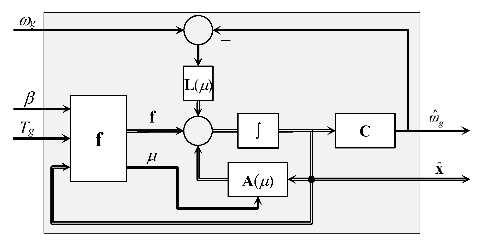
The model derived in the previous section is used to design an observer to estimate non-measurable variables [39] such as, for instance, effective wind speed. The scheme is presented in Figure 2.
The observer has two main characteristics: on the one hand, it is nonlinear in the inputs [40]; on the other hand, the matrix A has variable parameters [41]. A block diagram of the observer is shown in Figure 3.

4.2. Determination of the Observer Gain

The equations that describe the observer are given by
x ^ ˙ ( t )   = A ( μ ) x ^ ( t ) + f [ μ , x ^ ( t ) , u ( t ) ] + L ( μ )   [ y ( t ) y ^ ( t ) ] , y ^ ( t ) = c T x ( t )
which can be rewritten as
x ^ ˙ ( t )   = [ A ( μ ) L ( μ )   c T ]   x ^ ( t ) + f [ μ , x ^ ( t ) , u ( t ) ] + L ( μ ) y ( t ) ,
where the observer gain is L = [l1 l2 l3]T, and the system matrix is defined by
A ( μ ) L ( μ )   c T = a 11 a 12 a 13 a 21 a 22 a 23 a 31 a 32 0 1 1 / μ   1 / μ μ 1 1 μ 1 1 + 0 l 1 0 0 l 2 0 0 l 3 0 = a 11 a 12 / μ + l 1 a 13 / μ μ   a 21 a 22 + l 2 a 23 μ   a 31 a 32 + l 3 0
such that the characteristic equation is defined by the polynomial
P ( s ) = det [ s I A ( μ ) + L ( μ )   c T ] = det s a 11 a 12 / μ + l 1 ( μ ) a 13 / μ μ   a 21 s a 22 + l 2 ( μ ) a 23 μ   a 31 a 32 + l 3 ( μ ) s = 0 ,
which can also be represented by
P ( s ) = R ( s ) + μ   T ( s ) = 0 ,
where R, T, and P are the polynomials
R ( s ) = s 3 + r 1   s 2 + r 2   s + r 3 , T ( s ) = t 0   s + t 1 ,   and P ( s ) = s 3 + p 1   s 2 + p 2   s + p 3 .
with the coefficients
r 1   = l 2 a 11 a 22 , r 2 = a 11 l 2 + a 23 l 3 + a 11 a 22 ( a 13 a 31 + a 23 a 32 + a 12 a 21 ) , r 3 = a 13   a 31   l 2 + ( a 13   a 21 a 11   a 23 )   l 3 + a 13   a 31   a 22 + a 23   a 32   a 11 ( a 12   a 23   a 31 + a 13   a 32   a 21 ) , t 0   = a 21   l 1 ,   and t 1 = a 23   a 31   l 1 .
The idea behind the observer design is to keep the positions of the observer poles constant for all values of μ. Hence, pole placement [42] is an adequate design method. The given poles specify the coefficients of the polynomial P(s), which are always constant. The coefficient comparison leads to
p 1 = r 1 , p 2 = r 2 + μ     t 0 ,   and p 3 = r 3 + μ     t 1 .
Finally, the observer gain is obtained from
l 1 ( μ ) l 2 ( μ ) l 3 ( μ ) = 0 1 0 μ   a 21 a 11 a 23 μ   a 23   a 31 a 13   a 31 a 13   a 21 a 11   a 23 1 p 1 + a 11 + a 22 p 2 + a 13 a 31 + a 23 a 32 + a 12 a 21 a 11 a 22 p 3 + a 12   a 23   a 31 + a 13   a 21   a 32 ( a 13   a 22   a 31 + a 11   a 23   a 32 ) .
The values of the wind speed cut-in (vci) and cut-out (vco) are the span limits for the operation of the wind turbine. Consequently, the variable μ is also constrained in light of
μ m i n = v c i R μ v c o R = μ m a x .
In addition, ωg, Ta, and Tg are also bounded. This implies the boundness of a11 and a22, which are variable due to (16). The consequence of a variable matrix A is that (26) must be continuously recomputed in the runtime.

4.3. Stability and Convergence

The dynamic representation of the observer (19) is now rewritten as
x ^ ˙ ( t )   = [ A ( μ ) L ( μ )   c T ]   x ^ ( t ) + g [ μ , x ^ ( t ) , u ( t ) , y ( t ) ] ,
where function g is
g [ μ , x ^ ( t ) , u ( t ) , y ( t ) ]   = f [ μ , x ^ ( t ) , u ( t ) ] + L ( μ )   y ( t ) .
Under the consideration of the model parameters and an optimal control law for the generator control, the function g can be expressed by
g ( μ , x , u , y ) =   K J r μ   C p ( x 1 , β ) x 1 + l 1 ( μ )   ω g K o p t n x J g ω g 2 + l 2 ( μ )   ω g l 3 ( μ )   ω g .
The conventional analysis considers the stability of [A(μ)−L(μ) cT] and imposes the condition
| | g ( μ , x , u , y ) | |   γ | | x | |  
with γ > 0 for g (see, e.g., [43,44,45]). For the stability of [A(μ) − L(μ) cT], the characteristic Equation (22) is analysed. It is important to note that due to (27) and (16), P(s) is an interval polynomial with
[ p 0 p 0 + ] = [ 1   1 ] ,   [ p 1 p 1 + ] = [ r 1 , m i n   r 1 , m a x ] ,   [ p 2 p 2 + ] = [ ( r 2 , m i n + μ m i n t 0 )   ( r 2 , m a x + μ m a x t 0 ) ] ,   and   [ p 3 p 3 + ] = [ ( r 3 , m i n + μ m i n t 1 )   ( r 3 , m a x + μ m a x t 1 ) ] .
This means that the observer is an interval observer [43,45,46]. The stability requires that the four Kharitonov’s polynomials [47]
P 1 ( s ) = s 3 + p 1 s 2 + p 2 s + p 3 ,   P 2 ( s ) = s 3 + p 1 s 2 + p 2 + s + p 3 + ,   P 3 ( s ) = s 3 + p 1 s 2 + p 2 s + p 3 + ,   and   P 4 ( s ) = s 3 + p 1 s 2 + p 2 + s + p 3
are Hurwitz.
According to the definition of the state variables, ||x|| is given by
| | x | | = λ 2 + ω g 2 + Δ θ 2 ,
and for g, one has
| | g | | = K   C p ( β , x 1 ) μ x 1 + l 1   ω g 2 + K o p t ω g 2 J g + l 2   ω g 2 + l 3 2   ω g 2 .
Cp, λ, and μ are always bounded. For partial load operation, ωg < ωg,rated and, by assuming perfect pitch control in full load operation, it follows ωg = ωg,rated. Hence, it is always possible to find a finite γ such that
γ > K   C p , m a x μ m a x / λ m i n + l 1   ω g , r a t e d 2 + ( K o p t / J g + l 2 ) 2 + l 3 2 ω g , r a t e d 2 λ m i n 2 + ω g , m i n 2 + Δ θ g , m i n 2 ,
where the right side is the upper bound for the system and (31) holds.

5. Applications

The proposed model can be used for several objectives. However, only two applications are presented in this work, namely, the control during the partial load operation, which is achieved by using tip-speed ratio control, and the estimation of the effective wind speed. Both approaches are described in the following.

5.1. Tip-Speed Ratio Control in Partial Load Operation

In the partial load operation, the tip-speed ratio is maintained constant at the value of λ* in order to maximise the power coefficient Cp and, consequently, the energy conversion. There are several approaches to this objective (see, e.g., [21,48,49]), but one of them is the tip-speed ratio control (TSRC), which uses a closed-loop system with λ* as the set point (see Figure 4).
The control law is given by
T g i   = T   g , r a t e d f c o n ( λ * λ ^ ) ,
where fcon is the controller function, as, for example, the PI control law (proportional-integral), which in such a case can be expressed in the parallel decoupled form as
f c o n ( λ * λ ^ )   = K m [ K p ( λ * λ ^ ) + K i ( λ * λ ^ )   d t ]
with Kp and Ki as proportional and integral gains, respectively. Km is an adaptive adjustment factor defined as
K m   = K 1 + K 2 sech ( K 3 ( λ * λ ^ ) )
such that Km = K1 for very large λ * λ ^ and Km = K1 + K2 for small λ * λ ^ .
Notice that when the control error is equal to zero, the system reaches the rated values, and the linear controller provides a control variable equal to zero. However, the input torque may not be zero. Thus, this situation is avoided in the control law (37), because, when the controller output is zero, the torque is equal to its rated value.

5.2. Estimation of Effective Wind Speed

From (2), it follows that the wind speed can be calculated by
v w   = R λ ω r ,
where ωr and λ are not measurable variables, but they can be estimated by the observer, i.e.,
v ^ w   = R λ ^ ω ^ r .
This idea is schematised in Figure 5, where all state variables provided by the observer are brought into play to estimate the effective wind speed.

6. Numerical Example

The effectiveness of the proposed modelling approach is demonstrated by a numerical example regarding the wind speed estimation (Figure 5) as well as the control in the partial load operation (Figure 4). The numerical example is carried out by using a 20 MW reference wind turbine from [50], which has been modified and studied for modelling and control in [51,52].
The controller and observer designs, the simulation of both, and the evaluation of the results are carried out using MATLAB® and Simulink®. The simulation of the wind turbine is undertaken using OpenFAST (formerly known as FAST) [53].

6.1. Parameters and Rated Values

The relevant parameters of the reference wind turbine for model (5) are presented in Table 1, and the rated values are summarised in Table 2.

6.2. Model Calibration

It is shown in Section 3 that the steady-state model provides important information to obtain unknown parameters as well as variables in the stationary state. Steady-state variables depend on the wind speed. Thus, the steady-state values for the rated wind speed are summarised in Table 3. Steady-state values for other wind speeds are shown in the form of curves, in particular, in Figure 6.
From (17), it follows
B r = B g = n x ( T a n x T g ) ( 1 + n x 2 )   ω g   = 0.03 ,
which leads to
Be = 806.003.
Applying these values to (14) and (15), Δθ and λ are computed to be Δθ = 4.067 × 10⁻⁶ rad and λ = 9.4428. The range for μ is
0.0325 < μ < 0.1816 ,
and the steady-state value μ is 0.0793.
These stationary values dependent on the wind speed are obtained at the overrated wind for the corresponding value of the pitch angle according to the pitch angle locus of Figure 6a. In Figure 6b, the variable parameter Be, with the axis on the left, and the steady-state values of μ, with the axis on the right are presented against the wind speed changing from 0 to 25 m/s. Finally, the stationary twist angle of the low-speed shaft (Δθ), with the axis on the left, and the tip-speed ratio, with the axis on the right are shown in Figure 6c against a wind speed changing from 0 to 25 m/s.

6.3. Observer Design

As mentioned previously, the observer is designed by using the pole placement approach to maintain the poles always in the same position independently of the wind speed changes (or changes in the variable μ, which also varies with the wind speed).
The selection of the observer’s poles is carried out, taking into consideration reaction time, convergence, and estimation errors. Compromising all these criteria, the poles have been chosen after several runs of the simulation code. The final decision yields po1 = −50.0, po2 = −115.0, and po3 = −10.0.
The observer matrix gain is computed in the runtime for each value of the wind speed. Thus, the three elements of the matrix gain are obtained in the form of time series, which are portrayed in Figure 7.
It can be observed that while l1, which is strongly related to λ, presents important variability between 125.8 and 241.09, l2 and l3 remain practically constant for the whole time with average values of 174.73 and 1.19, respectively.

6.4. Tip-Speed Ratio Control in Partial Load Operation

The control system design for partial load operation has been presented in the previous section and is schematised in Figure 4. From Table 2, it follows that the set point for the tip-speed ratio is λ* = 10.115. The aim of the control system in partial load operation is to maximise power extraction. The metric used to evaluate the control performance is the converted average energy expressed in kWh. For the comparison, the classic optimal torque control law given by
T g i   = π 2   ρ a R 5 C p , m a x n x 2 ( λ * ) 3 ω g 2 = K o p t   ω g 2
is used, and, according to the information presented in Table 1 and Table 2, the optimal gain Kopt is computed to be 1132.9. The PI controller of the TSRC has been tuned but not optimized, and the corresponding parameters are Kp = 1536.2 and Ki = –0.1732. In addition, an anti-windup mechanism based on the back calculation concept [54] has been activated with a gain of Ka = 10.5. Parameters K1, K2, and K3 in the control law (39) are set to 0.43, 0.57, and 0.1, respectively.
The power curves obtained in the simulation under both control laws are portrayed in Figure 8. It corresponds to a calculated energy of 3385 kWh for optimal torque control and 3667 kWh for tip-speed ratio control.
It is very important to emphasise that the intention is not to compare the performances of both control algorithms but to show that the tip-speed ratio control in the proposed configuration can be implemented with satisfactory and comparable results by using the described approach.

6.5. Estimation of State Variables

The most important state variable to be estimated is the tip-speed ratio since the model has been modified in order to obtain it. On the other hand, a good estimation of this variable is needed for successful generator control in partial load operation, as well as for wind speed estimation.
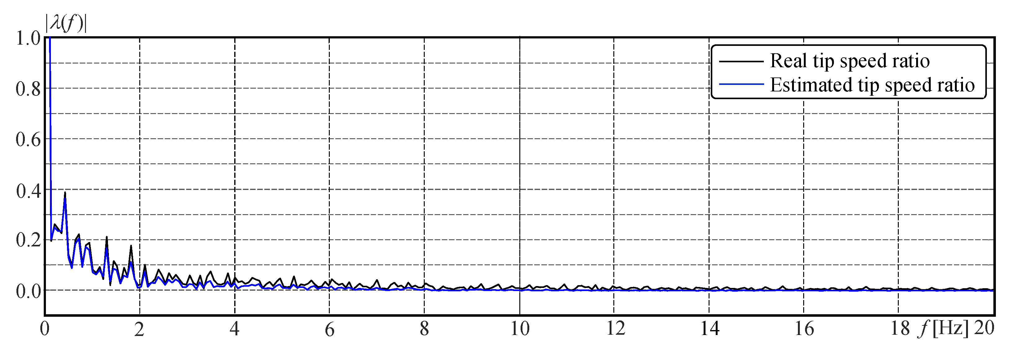
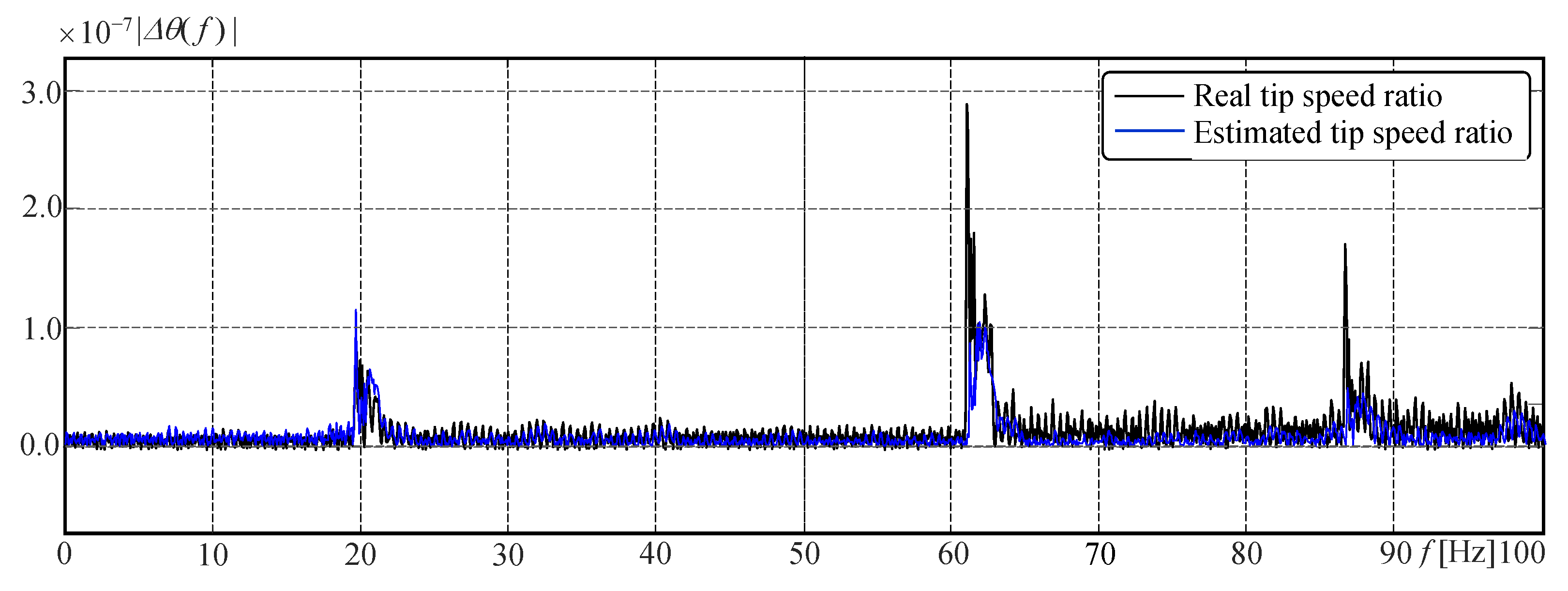
The simulation results comparing the real tip-speed ratio obtained from the simulation of the high-definition model with the observer output are presented in Figure 9, where the delay manifested in its reaction can be appreciated. Moreover, the observer also has a smoothing characteristic, which is not only visible in Figure 9, but is more evident in the frequency spectrum of Figure 10. Hence, the qualitative analysis indicates a satisfactory result. A more detailed evaluation is provided by using a quantitative analysis in 6.6.
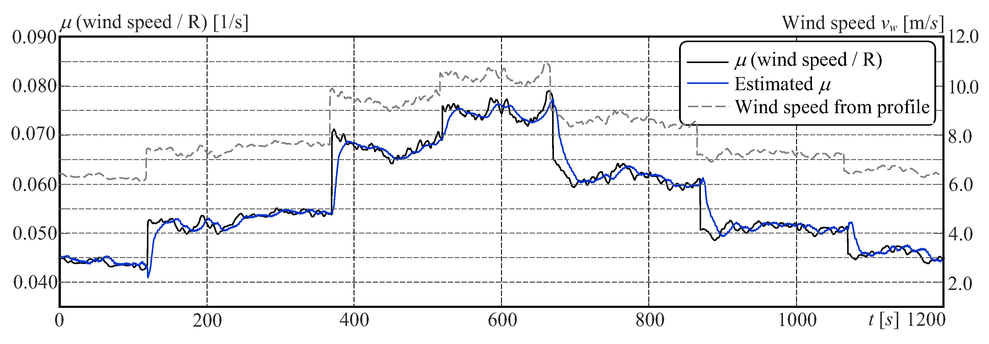
The variable μ, which is dependent on the unknown wind speed as shown in (2), also affects the tip-speed ratio λ. This dependence corresponds to an R-squared value of 0.9695, and is shown in Figure 11. Hence, it is also necessary to estimate μ, whose result is depicted in Figure 12.
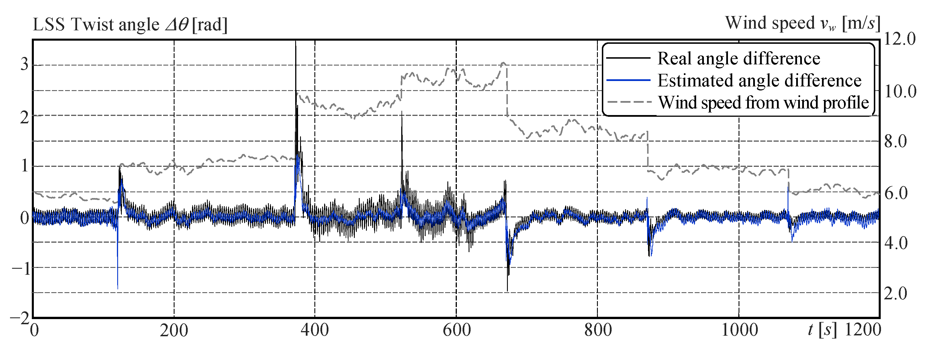
The twist angle of the low-speed shaft Δθr is more difficult to verify because it is not directly obtainable from the high-resolution model. However, it can be studied from two points of view. The first one is to calculate Δθ from measurable data. This is shown in Figure 13. The smoothing feature of the observer is also clearly exposed in the frequency spectrum of Figure 14.
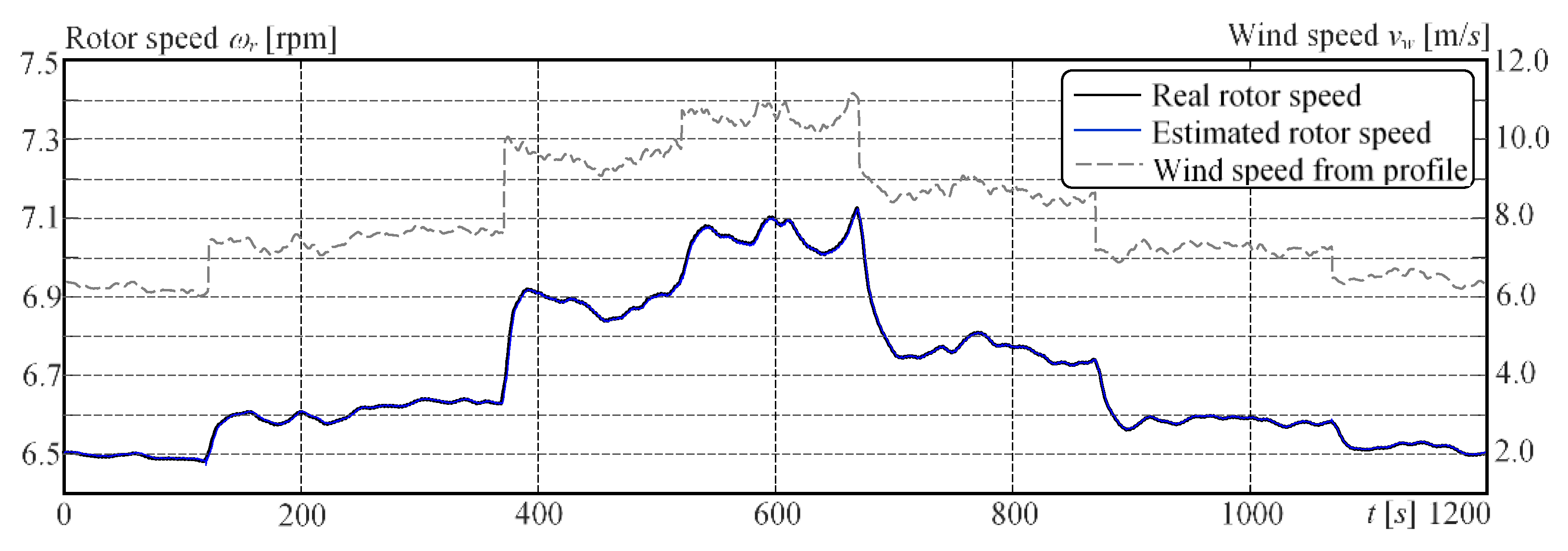
The other way is to use the rotor speed. Notice that the rotor speed is obtained from the third equation of (1) by using the derivative of the twist angle and the generator speed. The generator speed has a very high degree of agreement, because it is a measurable variable used as an input to the observer. Hence, the estimated rotor speed would be incorrect if the estimated derivative of the twist angle was erroneous. However, this is not the case, as can be appreciated in Figure 15 as well as in Table 4.
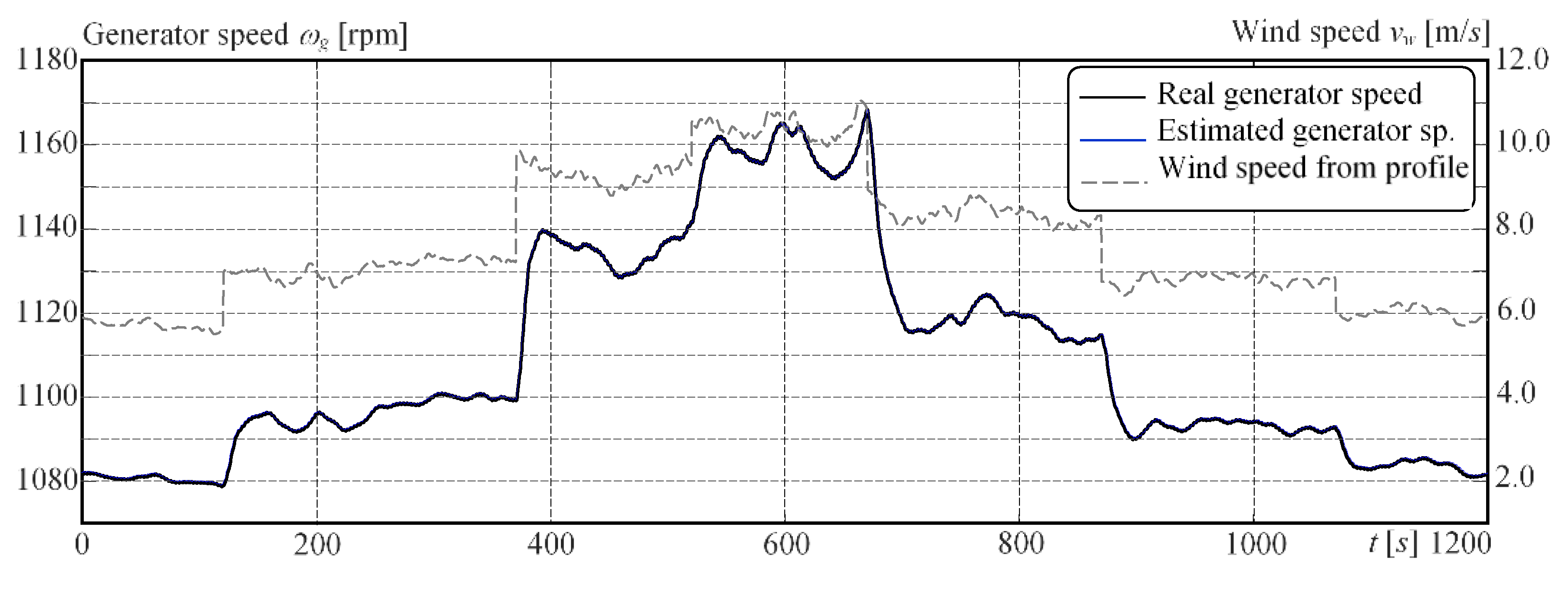
In the case of the generator speed, a very high agreement between the real signal and estimates is expected since this is a measurable output of the system and an input to the observer. This is confirmed in Figure 16 as well as in Table 4, where the cross-correlation factor equal to one supports the expectation.
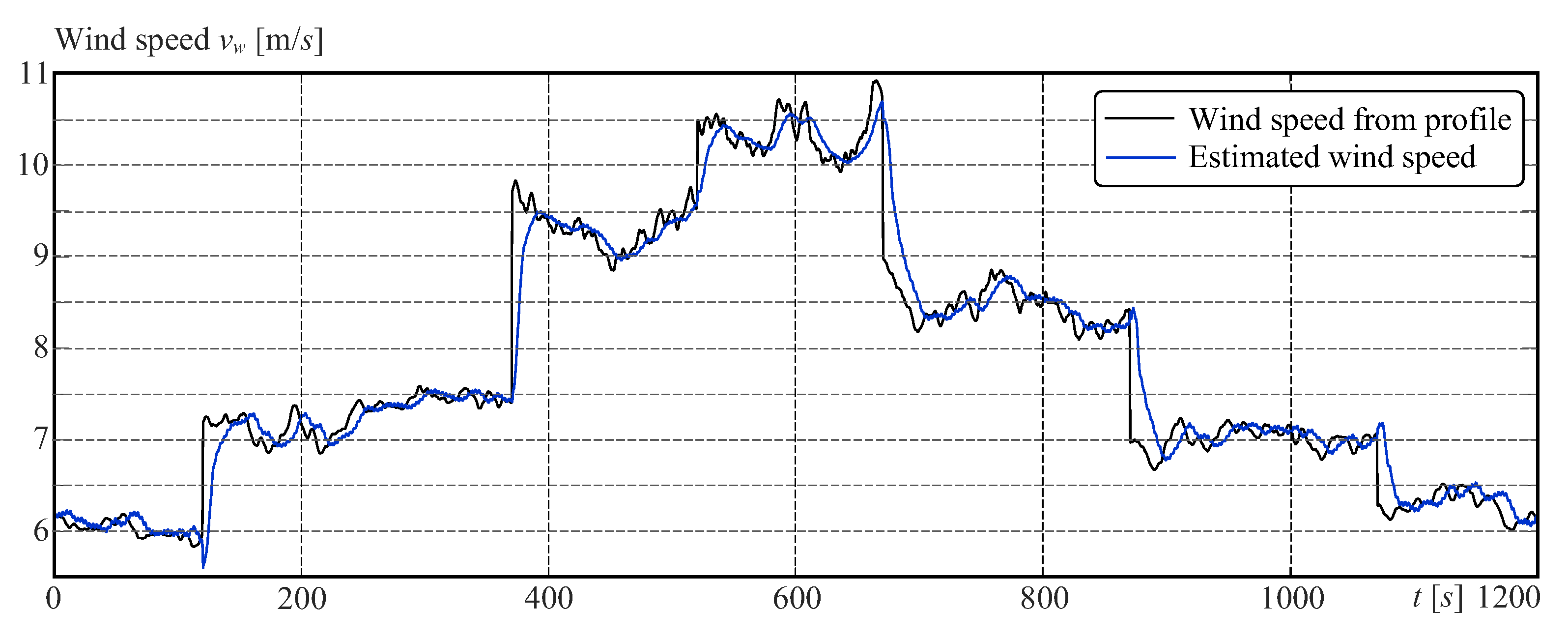
Finally, the wind speed is estimated by using Equation (41), which is an equation that is based on two estimated state variables, and therefore, a poor agreement might be anticipated. However, the result can be considered highly satisfactory, as evidenced by Figure 17 and the last column of Table 4.

6.6. Quantitative Analysis of the Observer Performance

To quantify the performance of the model and the designed observer, several metrics for estimation goodness are computed and assessed. Table 4 provides a summary of the findings.
For R-squared (R2), the closer the value is to 1, the better the observer’s behaviour is. For all other metrics, the best results are characterised by values closer to 0. The advantage of MSE over MAE is that MSE punishes significant errors more severely. On the other hand, RMSE maintains the same units as the original signal, which does not happen with MSE. Finally, RMSE provides the offset difference between both signals in the same unit (0 for no offset, i.e., full coincidence), and R-squared highlights the temporal shifting between both signals (1 for full coincidence). Satisfactory results from the point of view of the SME (Subject Matter Experts, [55,56]) are given for a threshold above 0.90 for R-squared, and a threshold below 0.50 for RMSE.
Under such conditions, the results of Table 4 are satisfactory in general, with acceptable values of RMSE and R-squared for λ. The R-squared value of Δθr is low, but the variable is not particularly important for the general control system.

7. Conclusions

This contribution describes a new modelling idea that includes the tip-speed ratio as a state variable in the dynamic model of the drivetrain. This concept leads to a model with interval parameters, for which an interval observer is designed.
The advantage of this model lies in the fact that the effective wind speed, which is normally unavailable, is not necessary to compute the tip-speed ratio. Contrarily, the estimates provided by the observer can be used to estimate the effective wind speed.
Another application is the torque control in partial load operation by using a tip-speed ratio control loop, where the tip-speed ratio estimated by the interval observer is fed back to the controller.
Both applications, i.e., effective wind speed estimation and tip-speed ratio control, are studied using a 20 MW reference wind turbine. The simulation results show the practical applicability of the model. It is important to note that the high-definition model of the reference wind turbine is reduced to a very simple third-order model. Despite this, the results have been very satisfactory. It is therefore to be expected that by using models of higher order, the outcomes can be even better.
Hence, the next step in the investigation is to consider models that include additional degrees of freedom. In particular, three-mass models, which include an additional degree of freedom for the blades, have been considered to date. Moreover, control algorithms will be implemented for testing in real-time operation using a Hardware-in-the-Loop (HiL) facility [57].

Author Contributions

A.G. Conceptualization, methodology, investigation, data curation, and writing (original draft). Y.Y.N. Investigation, formal analysis, validation and writing (review and editing). All authors have read and agreed to the published version of the manuscript.

Funding

This work has been financed by the Federal Ministry of Economic Affairs and Climate Action (BMWK).

Institutional Review Board Statement

Not applicable.

Informed Consent Statement

Not applicable.

Data Availability Statement

Data are available upon request from the corresponding author if allowed by the funding agency.

Conflicts of Interest

The authors declare no conflict of interest. The funders had no role in the design of the study, in the collection, analyses, or interpretation of data, in the writing of the manuscript, or in the decision to publish the results.

Nomenclature

Parameters
BgGenerator viscouse friction coefficient, Nm s/rad
BeEquivalent friction coefficient, Nm s/rad
BrRotor viscouse friction coefficient, Nm s/rad
CpPower coefficient, --
Cp,maxMaximum value of the power coefficient, --
DrDamping coefficient of the low-speed shaft, Nm s/rad
KProportional constant, Nm/(rad/s)²
KoptOptimal proportional constant, Nm/(rad/s)²
KrStiffness coefficient for the low-speed shaft, Nm/rad
K1, K2, K3, Kp, Ki, KmController gains
JrRotor mass moment of inertia, kg m²
JgGenerator mass moment of inertia, kg m²
nxGearbox ratio, --
Pm,ratedRated mechanical power, MW
RRotor radius, m
Ta,ratedRated aerodynamic torque, kg m²
Ta∞Steady-state value of the aerodynamic torque, kg m²
Tg,ratedRated generator torque, kg m²
Tg∞Steady-state value of the generator torque, kg m²
vciCut-in value for the wind speed, m/s
vcoCut-out value for the wind speed, m/s
vv,ratedRated value for the wind speed, m/s
ΔθSteady-state value for twist angle for the low-speed shaft, rad
γPositive bounding constant (Equation (31))
λ*Optimal tip-speed ratio
λSteady-state value for the tip-speed ratio
λminMinimum value for the tip-speed ratio
μSteady-state value for μ, Hz
μmaxMaximum value for μ, Hz
ηx, ηgEfficiency of gearbox and generator
ρaDensity of air, kg/m³
ωg,ratedRated value of the generator speed, rad/s
ωr,ratedRated value of the rotor speed, rad/s
ASystem matrix
cOutput vector
LObserver gain
aijElements of matrix A
liElements of observer gain L
R(s)Polynomial of Laplace variable s and coefficients ri
T(s)Polynomial of Laplace variable s and coefficients ti
P(s)Polynomial of Laplace variable s and coefficients pi
pi+, pi-Extreme coefficients for interval polynomial P(s)
Variables
PmMechanical power, MW
TaAerodynamic torque (on the low-speed shaft), kg m²
TgGenerator torque (on the low-speed shaft), kg m²
vvWind speed, m/s
xiState variables
βPitch angle, rad
ΔθTwist angle of the low-speed shaft, rad
λTip-speed ratio,--
μvv/R, Hz
ωgGenerator speed, rad/s
ωrRotor speed, rad/s
Functions
fconController function
fInput vector function
gInput vector function with output feedback

References

  1. Bianchi, F.D.; Mantz, R.J.; De Battista, H. Wind Turbine Control Systems; Springer: London, UK, 2007; ISBN 978-1-846-28-492-23-7. [Google Scholar] [CrossRef]
  2. Gambier, A. Control of Large Wind Energy Systems; Springer Nature: Basel, Switzerland, 2022; ISBN 978-3-030-84894-15-8. [Google Scholar]
  3. Boukhezzar, B.; Siguerdidjane, H. Nonlinear Control of a Variable-Speed Wind Turbine Using a Two-Mass Model. IEEE Trans. Energy Convers. 2010, 26, 149–162. [Google Scholar] [CrossRef]
  4. Dang, D.Q.; Wang, Y.; Cai, W. A multi-objective optimal nonlinear control of variable speed wind turbine. In Proceedings of the IEEE International Conference on Control and Automation, Christchurch, New Zealand, 9–11 December 2009; pp. 17–22. [Google Scholar] [CrossRef]
  5. Sami, M.; Patton, R.J. An FTC Approach to Wind Turbine Power Maximisation via T-S Fuzzy Modelling and Control. In Proceedings of the 8th IFAC Symposium on Fault Detection, Supervision and Safety of Technical Processes, Mexico City, Mexico, 29–31 August 2012; pp. 349–354. [Google Scholar] [CrossRef]
  6. Xiao, S.; Yang, G.; Geng, H. Nonlinear pitch control design for load reduction on wind turbines. In Proceedings of the International Power Electronics Conference, Hiroshima, Japan, 18–21 May 2014; pp. 543–547. [Google Scholar] [CrossRef]
  7. Schlipf, D.; Schlipf, D.J.; Kühn, M. Nonlinear model predictive control of wind turbines using LIDAR. Wind Energy 2012, 16, 1107–1129. [Google Scholar] [CrossRef]
  8. Jelavic, M.; Peric, N. Wind turbine control for highly turbulent winds. Automatika 2009, 50, 35–151. [Google Scholar]
  9. Pournaras, C.; Riziotis, V.; Kladas, A. Wind Turbine Control Strategy Enabling Mechanical Stress Reduction Based on Dynamic Model Including Blade Oscillation Effects. In Proceedings of the 2008 International Conference on Electrical Machines, Vilamoura, Portugal, 6–9 September 2008; pp. 1–6. [Google Scholar] [CrossRef]
  10. Muyeen, S.M.; Ali, M.H.; Takahashi, R.; Murata, T.; Tamura, J.; Tomaki, Y.; Sakahara, A.; Sasano, E. Comparative study on transient stability analysis of wind turbine generator system using different drive train models. IET Renew. Power Gener. 2007, 1, 131–141. [Google Scholar] [CrossRef]
  11. Friis, J.; Nielsen, E.; Bonding, J.; Adegas, F.D.; Stoustrup, J.; Odgaard, P.F. Repetitive model predictive approach to individual pitch control of wind turbines. In Proceedings of the 50th IEEE Conference on Decision and Control and European Control Conference (CDC-ECC), Orlando, FL, USA, 12–15 December 2011; pp. 3664–3670. [Google Scholar] [CrossRef] [Green Version]
  12. Slootweg, J.G.; de Haan, S.W.H.; Polinder, H.; Kling, W.L. General model for representing variable speed wind turbines in power system dynamics simulations. IEEE Trans. Power Syst. 2003, 18, 144–151. [Google Scholar] [CrossRef]
  13. Salman, S.; Teo, A. Windmill modeling consideration and factors influencing the stability of a grid-connected wind power-based embedded generator. IEEE Trans. Power Syst. 2003, 18, 793–802. [Google Scholar] [CrossRef]
  14. Jasniewicz, B.; Geyler, M. Wind turbine modelling and identification for control system applications. In Proceedings of the European Wind Energy Conference (EWEC), Brussels, Belgium, 14–17 March 2011; pp. 280–284. [Google Scholar]
  15. Moriarty, P.J.; Butterfield, S.B. Wind turbine modeling overview for control engineers. In Proceedings of the 2009 American Control Conference, Saint Louis, MO, USA, 10–12 June 2009; pp. 2090–2095. [Google Scholar] [CrossRef]
  16. Gonzalez-Longatt, F.; Regulski, P.; Novanda, H.; Terzija, V. Impact of shaft stiffness on inertial response of fixed speed wind turbines. Autom. Electr. Power Syst. 2012, 36, 191–198. [Google Scholar] [CrossRef]
  17. Ramtharan, G.; Jenkins, N.; Anaya-Lara, O.; Bossanyi, E. Influence of structural dynamic representations of FSIG wind turbines on electrical transients. Wind Energy 2007, 10, 293–301. [Google Scholar] [CrossRef]
  18. Bajpai, R.S.; Goyal, M.; Gupta, R. Modeling and control of variable speed wind turbine using laboratory simulator. J. Renew. Sustain. Energy 2015, 7, 053127. [Google Scholar] [CrossRef]
  19. Gambier, A. Dynamic Modelling of the Rotating Subsystem of a Wind Turbine for Control Design Purposes. IFAC-PapersOnLine 2017, 50, 9896–9901. [Google Scholar] [CrossRef]
  20. Balasundar, C.; Sudharshanan, S.; Elakkiyavendan, R. Design of an optimal tip speed ratio control MPPT algorithm for standalone WECS. Int. J. Res. Appl. Sci. Eng. Technol. 2015, 3, 442–450. [Google Scholar]
  21. Nasiri, M.; Milimonfared, J.; Fathi, S. Modeling, analysis and comparison of TSR and OTC methods for MPPT and power smoothing in permanent magnet synchronous generator-based wind turbines. Energy Convers. Manag. 2014, 86, 892–900. [Google Scholar] [CrossRef]
  22. Thongam, J.S.; Ouhrouche, M. MPPT control methods in wind energy conversion systems. In Fundamental and Advanced Topics in Wind Power; IntechOpen: Rijeka, Croatia, 2011; pp. 339–360. [Google Scholar] [CrossRef]
  23. Jena, D.; Rajendran, S. A review of estimation of effective wind speed based control of wind turbines. Renew. Sustain. Energy Rev. 2015, 43, 1046–1062. [Google Scholar] [CrossRef]
  24. Ortega, R.; Mancilla-David, F.; Jaramillo, F. A globally convergent wind speed estimator for windmill systems. Int. J. Adapt. Control. Signal Process. 2013, 27, 413–425. [Google Scholar] [CrossRef]
  25. Odgaard, P.F.; Stoustrup, J. Unknown input observer based estimation of wind speed for wind turbines control. In Proceedings of the 18th IFAC World Congress, Milan, Italy, 28 August–2 September 2011; pp. 1698–1703. [Google Scholar] [CrossRef] [Green Version]
  26. Østergaard, K.Z.; Brath, P.; Stoustrup, J. Estimation of effective wind speed. J. Phys. Conf. Ser. 2007, 75, 012082. [Google Scholar] [CrossRef] [Green Version]
  27. Khoshrodi, M.N.; Jannati, M.; Sutikno, T. A Review of Wind Speed Estimation for Wind Turbine Systems Based on Kalman Filter Technique. Int. J. Electr. Comput. Eng. 2016, 6, 1406–1411. [Google Scholar] [CrossRef]
  28. Chen, H.; Zhang, Y. Power System Optimization: Large-Scale Complex Systems Approaches; John Wiley & Sons: Singapore, 2016; ISBN 978-1-118-72478-1. [Google Scholar]
  29. Mahmoud, M.S.; Hassan, M.F.; Darwish, M.G. Large-Scale Systems; Marcel Dekker Inc.: New York, NY, USA, 1985; ISBN 978-082-477289-5. [Google Scholar]
  30. Leithead, W.E.; de la Salle, S.A.; Reardon, D.; Grimble, M.J. Wind turbine modelling and control. In Proceedings of the International Conference on Control’91, Edinburgh, UK, 25–28 March 1991; pp. 1–6. [Google Scholar]
  31. Girsang, I.P.; Dhupia, J.S.; Muljadi, E.; Singh, M.; Pao, L.Y. Gearbox and Drivetrain Models to Study Dynamic Effects of Modern Wind Turbines. IEEE Trans. Ind. Appl. 2014, 50, 3777–3786. [Google Scholar] [CrossRef]
  32. Fortmann, J. Modeling of Wind Turbines with Doubly Fed Generator System; Springer: Wiesbaden, Germany, 2014; ISBN 978-3658-06882-0. [Google Scholar] [CrossRef]
  33. Rotea, M.A. Logarithmic Power Feedback for Extremum Seeking Control of Wind Turbines. IFAC-PapersOnLine 2017, 50, 4504–4509. [Google Scholar] [CrossRef]
  34. Burton, T.; Jenkins, N.; Sharpe, D.; Bossanyi, E. Wind Energy Handbook, 2nd ed.; John Wiley & Sons: Chichester, UK, 2011; ISBN 978-1-119-99271-4. [Google Scholar]
  35. Dekkers, R. Steady-state model. In Applied Systems Theory, 2nd ed.; Springer Nature: Cham, Switzerland, 2014; pp. 173–192. [Google Scholar] [CrossRef] [Green Version]
  36. Aljafari, B.; Stephenraj, J.P.; Vairavasundaram, I.; Rassiah, R.S. Steady State Modeling and Performance Analysis of a Wind Turbine-Based Doubly Fed Induction Generator System with Rotor Control. Energies 2022, 15, 3327. [Google Scholar] [CrossRef]
  37. Bonfiglio, A.; Delfino, F.; Gonzalez-Longatt, F.; Procopio, R. Steady-state assessments of PMSGs in wind generating units. Int. J. Electr. Power Energy Syst. 2017, 90, 87–93. [Google Scholar] [CrossRef] [Green Version]
  38. Johnson, K.; Pao, L.; Balas, M.; Kulkami, V.; Fingersh, L. Stability analysis of an adaptive torque controller for variable speed wind turbines. In Proceedings of the 3rd IEEE Conference on Decision and Control, Nassau, Bahamas, 14–17 December 2004; pp. 4087–4094. [Google Scholar] [CrossRef]
  39. Trinh, H.; Fernando, T. Functional Observers for Dynamical Systems 420; Springer: Berlin, Germany, 2012; ISBN 978-3-642-26955-4. [Google Scholar]
  40. Boutat, D.; Zheng, G. Observer Design for Nonlinear Dynamical Systems: Differential Geometric Methods 487; Springer Nature: Cham, Switzerland, 2021; ISBN 978-3-030-73742-9. [Google Scholar]
  41. Bullinger, E.; Ilchmann, A.; Allgöwer, F. A Simple Adaptive Observer for Nonlinear Systems. IFAC Proc. Vol. 1998, 31, 781–786. [Google Scholar] [CrossRef] [Green Version]
  42. Ellis, G. Observers in Control Systems: A Practical Guide; Academic Press: San Diego, CA, USA, 2002; ISBN 978-0-122-37472-2. [Google Scholar]
  43. Gouzé, J.; Rapaport, A.; Hadj-Sadok, M. Interval observers for uncertain biological systems. Ecol. Model. 2000, 133, 45–56. [Google Scholar] [CrossRef]
  44. Khan, A.; Xie, W.; Zhang, L.; Liu, L. Design and applications of interval observers for uncertain dynamical systems. IET Circuits Devices Syst. 2020, 14, 721–740. [Google Scholar] [CrossRef]
  45. Oubabas, H.; Djennoune, S.; Bettayeb, M. Interval sliding mode observer design for linear and nonlinear systems. J. Process Control 2018, 61, 12–22. [Google Scholar] [CrossRef]
  46. Khan, A.; Xie, W.; Zhang, B.; Liu, L.-W. A survey of interval observers design methods and implementation for uncertain systems. J. Frankl. Inst. 2021, 358, 3077–3126. [Google Scholar] [CrossRef]
  47. Bhattacharyya, S.P.; Chapellat, H.; Keel, L.H. Robust Control. The Parametric Approach; Prentice Hall: Upper Saddle River, UK, 1995; ISBN 978-0137815760. [Google Scholar]
  48. Ciri, U.; Leonardi, S.; Rotea, M.A. Evaluation of log-of-power extremum seeking control for wind turbines using large eddy simulations. Wind Energy 2019, 22, 992–1002. [Google Scholar] [CrossRef]
  49. Gambier, A.; Nazaruddin, Y.Y. Wind Turbine Control in Partial Load Operation by Using the Optimization Algorithms from the Deep Learning Techniques. In Proceedings of the 2022 International Automatic Control Conference, Kaohsiung, Taiwan, 3–6 November 2022. [Google Scholar] [CrossRef]
  50. Ashuri, T.; Martins, J.R.R.A.; Zaaijer, M.B.; van Kuik, G.A.M.; van Bussel, G.J.W. Aeroservoelastic design definition of a 20 MW common research wind turbine model. Wind Energy 2016, 19, 2071–2087. [Google Scholar] [CrossRef]
  51. Chamoli, S.; Gambier, A. Modelling, Parametrization and Observer Design of a 20 MW Reference Wind Turbine for Control Purposes. J. Phys. Conf. Ser. 2020, 1618, 022031. [Google Scholar] [CrossRef]
  52. Gambier, A.; Meng, F. Control System Design for a 20 MW Reference Wind Turbine. In Proceedings of the 12th Asian Control Conference, Hong Kong, China, 19–21 August 2019; pp. 258–263. [Google Scholar] [CrossRef]
  53. Jonkman, J.; Jonkman, B.J. FAST modularization framework for wind turbine simulation: Full-system linearization. J. Phys. Conf. Ser. 2016, 753, 082010. [Google Scholar] [CrossRef] [Green Version]
  54. Visioli, A. Practical PID Control; Springer: London, UK, 2006; ISBN 978-1-84628-586-8. [Google Scholar]
  55. Schwer, L.E. Validation metrics for response histories: Perspectives and case studies. Eng. Comput. 2007, 23, 295–309. [Google Scholar] [CrossRef]
  56. Teferra, K.; Shields, M.D.; Hapij, A.; Daddazio, R.P. Mapping model validation metrics to subject matter expert scores for model adequacy assessment. Reliab. Eng. Syst. Saf. 2014, 132, 9–19. [Google Scholar] [CrossRef]
  57. Kenko, D.G. A Real-time wind turbine simulation for pitch control purposes by using a hardware-in-the-loop approach. In Proceedings of the 21st International Conference on Modelling and Applied Simulation, Rome, Italy, 19−21 September 2022. [Google Scholar] [CrossRef]
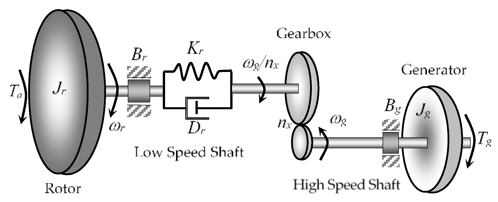
Figure 1. Drivetrain described by a two-mass system with a gearbox.
Energies 15 09454 g001
Figure 2. Observer configuration for the estimation of state variables and effective wind speed.
Energies 15 09454 g002
Figure 3. Block diagram for the observer given in Figure 2.
Energies 15 09454 g003
Figure 4. Tip-speed ratio control based on the observer.
Energies 15 09454 g004
Figure 5. Estimation of the effective wind speed based on the observer.
Energies 15 09454 g005
Figure 6. (a) Locus of pitch angles; (b) parameter Be and variable μ; (c) steady-state twist angle Δθ, and tip-speed ratio λ.
Energies 15 09454 g006
Figure 7. Observer gains.
Energies 15 09454 g007
Figure 8. Time series of the extracted power under the control system in partial load operation.
Energies 15 09454 g008
Figure 9. Time series of the tip-speed ratio.
Energies 15 09454 g009
Figure 10. Single-side amplitude spectrum of the tip-speed ratio.
Energies 15 09454 g010
Figure 11. Relationship between λ and μ.
Energies 15 09454 g011
Figure 12. Time series of variable s.
Energies 15 09454 g012
Figure 13. Time series of the twist angle of the slow-speed shaft.
Energies 15 09454 g013
Figure 14. Single-side amplitude spectrum of the shaft twist angle.
Energies 15 09454 g014
Figure 15. Time series of the rotor speed.
Energies 15 09454 g015
Figure 16. Time series of the generator speed.
Energies 15 09454 g016
Figure 17. Time series of the wind speed profile and the estimated effective wind speed.
Energies 15 09454 g017
Table 1. Essential parameters of the 20 MW reference wind turbine.
ParameterNotationValuesUnits
Equivalent shaft spring constantKr6.94 × 109Nm/rad
Equivalent shaft damping constantDr4.97 × 107 Nm/(rad/s)
Gearbox rationx164--
Gearbox efficiency, generator efficiencyηx, ηg97.8, 96.1%
Rotor radiusR138m
Rotor mass moment of inertiaJr2919.66 × 106 kg m2
Mass moment of inertia of the generatorJg7248.32kg m2
Table 2. Rated values for the 20 MW wind turbine.
VariableNotationValuesUnits
Rated mechanical powerPm,rated21.191MW
Rated rotor speedωr,rated7.1567rpm
Rated generator speedωg,rated1173.7rad/s
Cut-in, rated, and cut-out wind speedvci, vw,rated, vco4.48, 10.92, 25 m/s
Rated aerodynamic torque (on the low-speed shaft)Ta,rated28434.7 kNm
Rated generator torque (on the high-speed shaft)Tg,rated169.76kNm
Maximum value of the power coefficient CpCp,max0.4812--
Optimal tip-speed ratio λ*10.115--
Density of airρa1.225kg/m3
Table 3. Steady-state values of the 20 MW wind turbine for the rated wind speed.
VariableNotationValuesUnits
Rotor speedωr0.7495rad/s
Generator speedωg122.912rad/s
Aerodynamic torque (on the low-speed shaft)Ta28,225.215 kNm
Generator torqueTg168.424kNm
Table 4. Quantitative evaluation of the model and observer performance.
ParameterλωgΔθrωrμvw
MAE (Mean Absolute Error)0.26760.00269.6978 × 10−64.7753 × 10−40.16460.0012
MSE (Mean Square Error)0.24381.555 × 10−53.3227 × 10−108.8550 × 10−70.09254.8028 × 10−6
R-squared (Square of the correlation)0.93361.00000.51301.00000.95280.9535
RMSE (Root Mean Squared Error)0.49380.00391.8228 × 10−59.4101 × 10−40.30410.0592
NRMSE (Normalized RMSE)0.07134.4283 × 10−50.06470.00170.05970.0022
Publisher’s Note: MDPI stays neutral with regard to jurisdictional claims in published maps and institutional affiliations.