Article

Reliability Analysis and Life Prediction of Aging LNG Unloading Arms Based on Non-Destructive Test Data

1
Department of Ocean Science and Engineering, Kunsan National University, Gunsan 54150, Republic of Korea
2
VARM Brain Co., Ltd., Seoul 05634, Republic of Korea
3
School of Architecture and Coastal Construction Engineering, Kunsan National University, Gunsan 54150, Republic of Korea
*
Author to whom correspondence should be addressed.
Energies 2022, 15(24), 9408; https://doi.org/10.3390/en15249408
Submission received: 12 October 2022 / Revised: 5 December 2022 / Accepted: 9 December 2022 / Published: 12 December 2022
(This article belongs to the Special Issue Frontiers in Advanced Energy Infrastructure Construction Technology)

Abstract

:
Unloading arms (ULAs) among seaport infrastructures are susceptible to deterioration posed by the effects of harsh marine environmental conditions. During infrastructure’s service life, the deterioration of structural integrity may increase the risk of failure of infrastructure, and should be taken into account during structural reliability assessment. In this study, a simple non-destructive test (NDT) was employed to examine the structural deterioration of ULAs which were installed over 30 years ago. Then, these aging ULAs were modeled by the finite-element program, using non-destructive test data to update the thickness dimensions of structural members. Next, a reliability assessment was conducted based on the stress distribution of the main structural components under external loads, which are calculated by their relation to wind speed. Moreover, the time-dependent reliability index curve was also built by considering the deterioration function to predict the failure probability of the particular components during the remaining lifetime. The study revealed that the present condition of the ULA system was satisfactory for current loading conditions. A reliability index predicted with deteriorations factors may be a rational and appropriate approach for the assessment of aging structures needed for efficient infrastructure management.

1. Introduction

Structural capacity is generally associated with the geometry and mechanical properties of a structural component. Unfortunately, during its service life, these factors may degrade due to environmental conditions, variation in load intensity over time, and quality of periodic maintenance. The periodic safety evaluation and damage assessment of existing aging structures considering the factors that influence structural deterioration is essential. In fact, the resistance deterioration of aging structures is a stochastic process and is related to the load history (e.g., long-term load intensity may result in fatigue causing cracking), environmental conditions, operation conditions, and protective measures (e.g., the loss of section thickness for structural elements by corrosion [1]). Wang et al. [2] proposed that the deterioration of the structural model consists of two components: gradual deterioration caused by environmental actions and shock deterioration caused by severe attacks of significant loads. Moreover, there is a lot of research published in the past two decades regarding the assessment of aging structures [3,4,5,6,7].
Reliability analysis is a frequently used tool in terms of estimating the probability of structural safety over time or after suffering the sudden natural events such as hurricanes, earthquakes, etc., [8,9], aimed at giving quantitative information to ensure that structures maintain performance within an acceptable safety level during their remaining service life. Concerning probabilistic approaches to assessments of deteriorating structures, there are many uncertainties that may directly threaten the safety of the in-service structures. A lot of research has been conducted on developing approaches for reliability analysis. Mori and Ellingwood [10] developed methods using structural reliability principles to evaluate the time-dependent reliability of reinforced or pre-stressed concrete structures. This work was further used by Enright and Frangopol to predict the probability of safety of deteriorating bridges [11]. Rodolfo Mussini et al. [12] developed a computational structural reliability model method in conjunction with the failure-assessment diagram method and the user-defined probability of detection curves of non-destructive testing is used. Bhargava et al. [13] conducted analysis to estimate the time-dependent failure probability for a corrosion-affected RC beam and investigated the influence of variability in degradation functions on structural failure probability. Liu et al. [14] studied different failure modes under hazards that cause both progressive and shock deteriorations of structural performance. In their study, a cumulative-time approach was presented for the probabilistic structural deterioration process. Moreover, the life-cycle cost assessment and optimization approach is a practical method to predict the time-to-repair and the number of repair operations on the degrading structures [15].
This study was conducted on the ULAs of an LNG terminal (hereinafter referred to as “A”) that has existed for more than 30 years in a certain area in Korea. Its storage capacity has continuously expanded over the past three decades. Seaports have largely created their sources of revenue from cargo handling, and marine unloading arms (ULAs) are an essential part. With high working intensity, infrastructure facilities, especially ULA systems, may have deteriorated. The assessment of the failure probability of this ULA system needs to be conducted. The simulation-based reliability analysis approach is considered as a suitable tool for doing this. A key factor in this approach is the model of the degraded structure, which must be accurately simulated. Ignoring the single and multiple deteriorations involved can overestimate or underestimate the safety of your infrastructure, which can lead to significant economic losses or sudden accidents. The scope of this paper is to perform a reliability analysis of existing aging ULAs subjected to stochastic wind load. NDT was performed to examine the loss of section thickness and structural integrity. In reliability analysis, the yield stress was used to define a limit state as well as random variables such as member thickness, elastic modulus, and wind speed. The wind speed distribution was derived from data collected in “A” harbor and it can be fitted into the lognormal distribution. The RSM (Response Surface Method)-based FORM (First Order Reliability Method) was used to calculate the reliability index. Then, a system reliability assessment of existing ULAs was given. Finally, a time-dependent reliability index of the most dangerous component was constructed to evaluate the failure probability of the ULA during the remaining lifetime.

2. Reliability Analysis

2.1. First-Order Reliability Method (FORM)

In reliability analysis, the limit state of interest must be defined first. This is the boundary between the safe and unsafe responses in the design parameter space. The limit-state function (LSF) can be written in the form of Equation (1), where R and S are the distributions of the resistance and load, respectively.
g X = R S
Considering the LSF of a structure, the failure probability P f can be defined as [16]:
P f = g X < 0 f X x 1 , x 2 , , x n d x 1 d x 2 d x n
where f X x 1 , x 2 , , x n is the joint probability density function for the uncertain input variables of the structure x 1 , x 2 , , x n and g X < 0 represents the structural failure region. The probability of failure in Equation (2) is solved by integral multiples and, obviously, it is a difficult challenge. FORM provides an approximate method. In the FORM process, the LSF g X = 0 was transformed into a corresponding limit-state surface g u = 0 in standard space (U-space). This process was conducted by Rosenblatt transformation [17]. In the next step, the most probable failure point on g u = 0 has to be determined in U-space. This is the point in the failure set with the largest probability density, that is, the closest point on the failure surface to the origin of the U-space. The shortest distance between the limit-state-boundary surface and the origin in the U-space is called the reliability index β.
Once the reliability index is obtained, the probability of failure P f is often represented in terms of the reliability index β given by:
P f = 1 Φ β
where the notion Φ is the cumulative distribution function (CDF) of the normally distributed random variable with mean of 0 and standard deviation of 1.

2.2. Response Surface Method (RSM)

For complex and implicit LSF, the RSM [18] provides a solution that allows expressing it in explicit form. The structural LSF in the RSM can be approximated using a quadratic polynomial function as follows:
g X a + i = 1 n b i x i + i = 1 n j = i n c i j x i x j
where x i ( i = 1, 2, …, n) is the space variable and a , b i , c i j are the coefficients. At the beginning of process, the mean point of the random variables is chosen as the initial point. An acceptable error margin ( ε ) is established so that performing the analysis is as simple as possible. The design test point of the structure of each iteration step can be determined by Equation (5) [19], where X i C is the center point, σ X i is the standard deviation of X i , h i is the width, I i is the scattering index, and i is the variable number.
X i = X i C ± h i σ X i I i
The analysis will be stopped at the k th iteration if the Equation (6) can be established, then it is possible to evaluate structural reliability.
β k β k 1 ε

2.3. Reliability of Aging Structure

In realistic structures, the deterioration of structures will lead to stochastic degradation of resistance and an increased load effect. As a result, performance evaluation of structures degraded over time has become more challenging for structural engineers owing to the stochastic nature of material properties and their random change over time. The relationship between resistance and load in reliability analysis of degraded structures can be seen in Figure 1. Note that there will be uncertainty both about the precise resistance and the rate of resistance loss with time. The load change with time is not considered in this paper. Instead, the load effect is established as a stochastic process to represent its randomness.
It is evident from Figure 1 that the failure probability of a structure increased with an increase in resistance loss ratio. Therefore, in the reliability analysis, it is necessary to consider the factors affecting the degradation of structural resistance. In realistic structures, there will be many resistance variables. Typically, these are random variables, and some may deteriorate with time. For example, for steel structures at seaports, the resistance of the structure is mainly dominated by the steel properties and moment of inertia including thickness (or cross-section) of the structural components. The probabilistic nature (uncertainty) of steel properties is represented by the probability density function. The uncertainty of structural thickness, besides being expressed by the probability density functions, also has its mean value defined as a function of time; see Figure 1. The structural thickness over time (residual thickness) can be inferred from the function of the amount of material loss due to corrosion. The bi-logarithmic model, Equation (7), is typically adopted to describe corrosion loss ( C ) as a function of the time of exposure, where A and B are two experimental parameters used differently by researchers. B can be called an environmental parameter. It depends on the atmosphere condition, the effect of protection level, etc., and is normally less than unity. A larger B value indicates a more severe environment, less effective protective measures, and vice versa. For the marine atmosphere, B = 0.69 [20]. A is the corrosion loss in the first year.
C t = A t B

2.4. System Reliability

Considering the correlation between components in the same system, the system failure probability can be conveniently calculated from the failure probabilities of the individual components. Basically, structural systems are of two types. The first is a structural system which consists of individually operated components, that is, if any of its components fail or lose function, the remaining components in the system still perform the function. Therefore, it can be seen as a functionally parallel system. In this case, the system failure probability can be calculated by the following equation:
P f , U L A s = 1 n P f , U L A i
where P f , U L A i is the failure probability of components in the same system. The second is a structural system which consists of components that work in mutual support as a distributed system. Normal operation of the distributed system is possible only when all its components are not damaged. This means that if any of its structural components fail or lose function, the operation is discontinued. This failure probability of system can be determined based on the failure probability of each component P f , i by the equation below:
P f , U L A = 1 1 n 1 P f , i

2.5. Target Reliability Index

The target reliability indices used by researchers are different and should be determined before performing structural reliability analysis. Such decisions will be based on the consequences of the failure, reference rules, inspection, and repair processes, etc. Ideally, the target reliability level so selected should minimize the total cost (i.e., optimize the cost of strengthening or replacement), but still comply with a certain minimum safety level. The target reliability indices corresponding to several reference rules were illustrated in Figure 2. Accordingly, the target reliability index applied in the design standards varies from 2.0 to 4.7, and is applied to general structures such as bridges, pipelines, seaport facilities, skyscrapers, etc. ISO [21] and Eurocode [22] standards recommend target reliability indices in the range of 3~4.7 for general structures. In the case of bridges, the damage to human life and property is high, so a target reliability of 3.0 or higher for the US and 3.1 or higher for Korea is applied. In this study, the ULA system was selected to perform the assessment. The failure of the ULA system here had no risk of human injury, minor economic consequences, and an insignificant impact on the environment. Therefore, it might be overly prudent and wasteful to apply reliability index levels corresponding to the reference rules listed above. Sotberg et al. [23] proposed a failure probability level, shown in Table 1, for the limit-state-based designs of pipelines. The low safety class in Table 1 can be used as a reference for target reliability evaluation. Accordingly, a failure probability level in the range of 10 2 10 3 corresponding to the target reliability index of 2.33–3.09 of the ultimate limit state was proposed as a reference for evaluation of reliability and safety assessment of unloading arms in this study. Specifically, in this study, the target reliability index was assumed to be 2.6, corresponding to failure probability 4.66 × 10 3 for performance evaluation of aging structures in the next section. As mentioned in Figure 2, the defined target reliability level is reasonable compared to the target reliability level in Japan, where earthquakes occur frequently.

3. Numerical Analysis

3.1. ULA

The structure selected for this study was the unloading arm (ULA) system installed in “A” Port 30 years ago. As shown in 
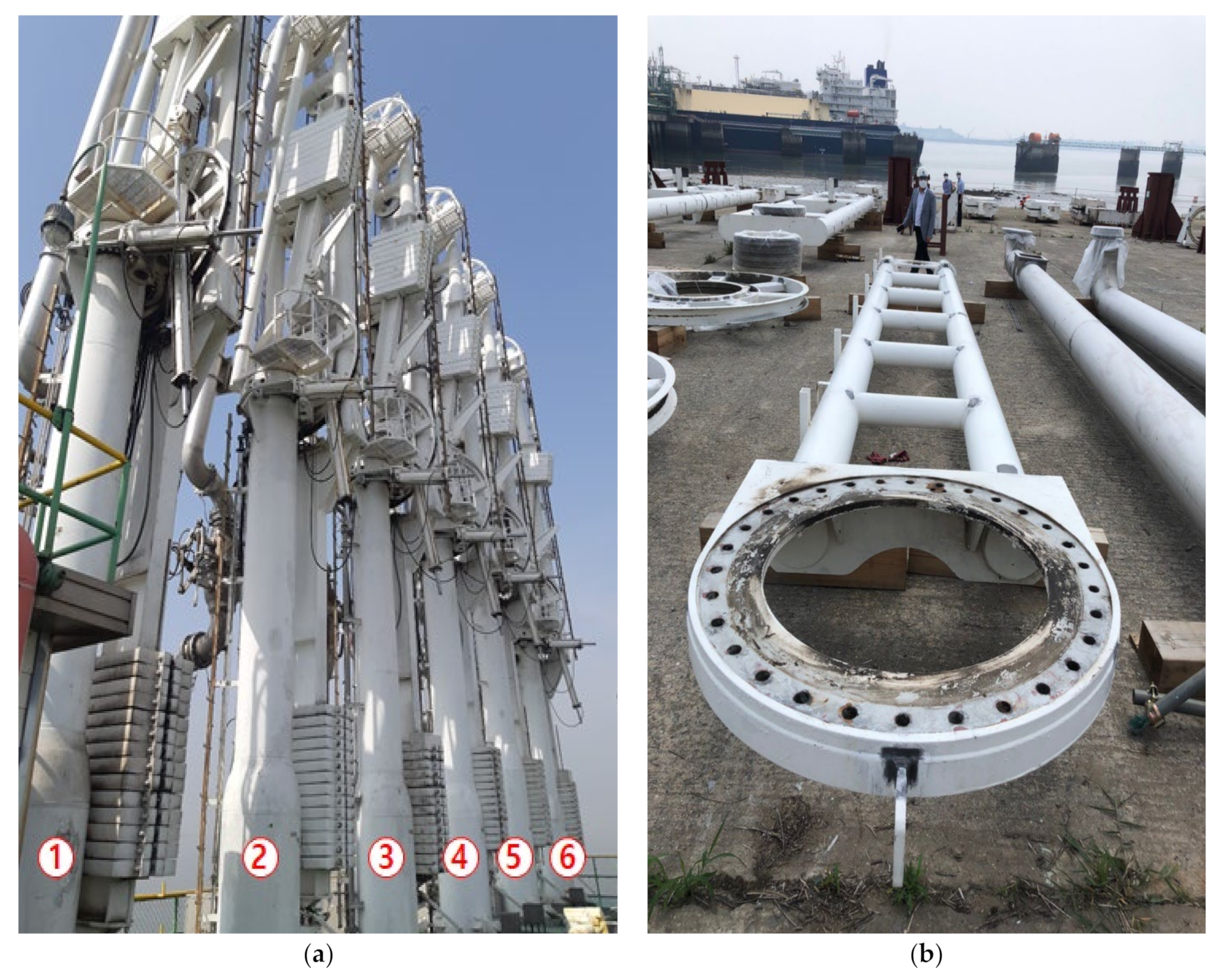
Table 2, it is a system composed of six marine arms divided into three main types. Here, the LNG (Liquefied Natural Gas), BOG (Boil-off gas), and Bunker unloading arms are denoted by the letters (L), (BOG), and (B/C), respectively. Since this system base was installed on a slab made of steel located about 14.5 m above sea level, it is hardly influenced by sea wave effects. 
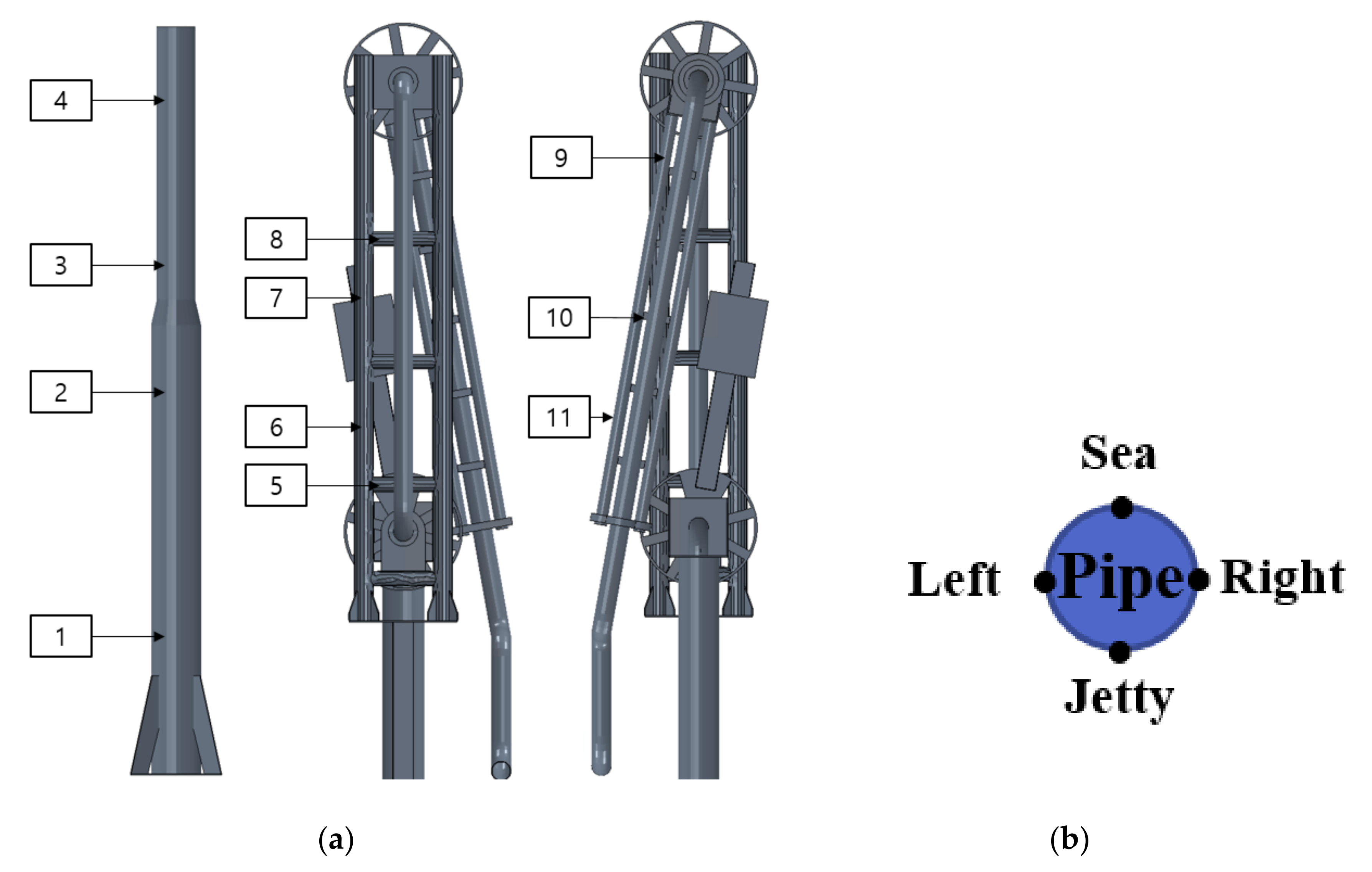
Figure 3a is a picture of the ULAs taken at “A” LNG terminal. When the components are disassembled as in 
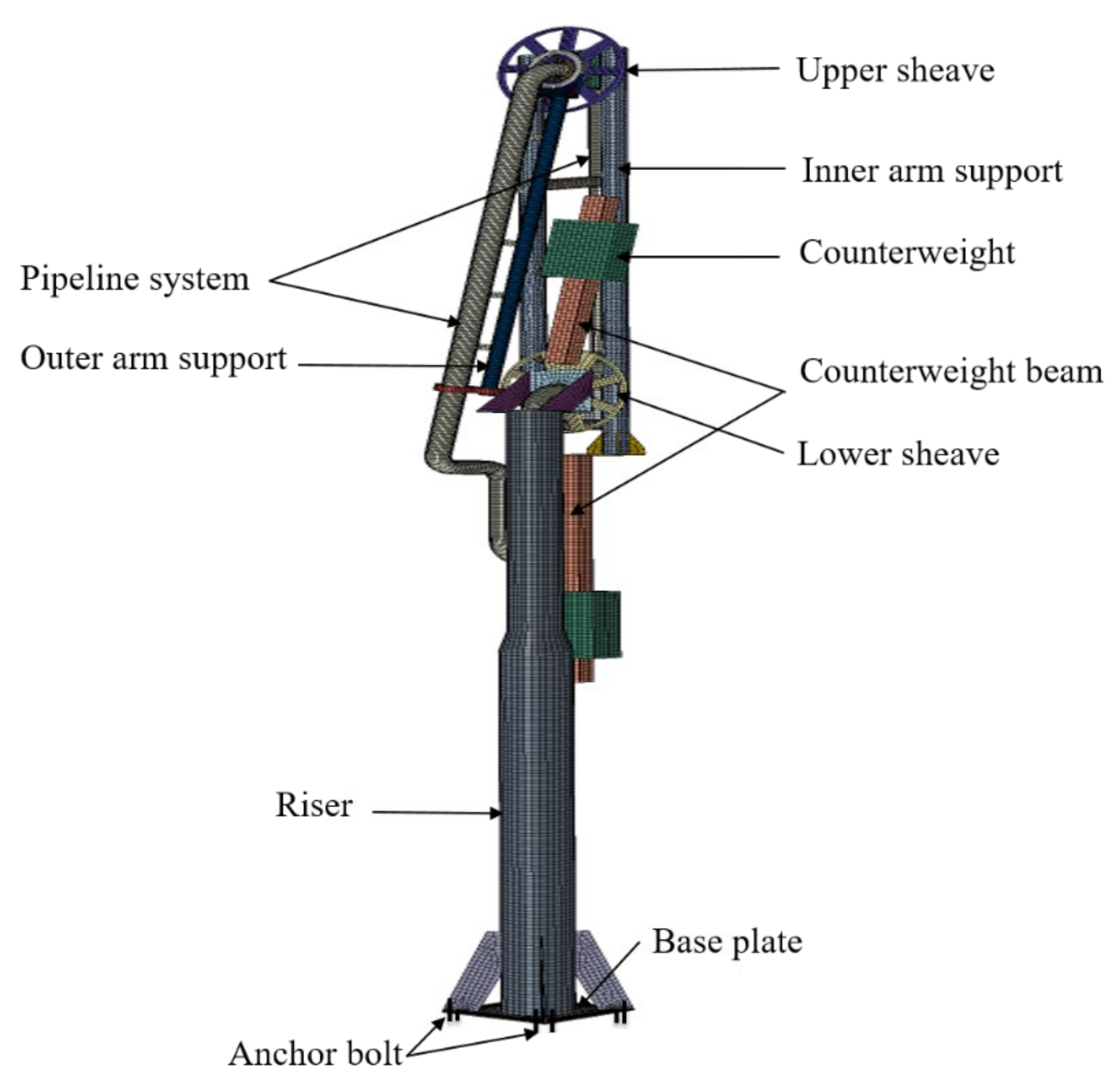
Figure 3b, it is also very convenient to perform non-destructive testing (NDT) to evaluate structural condition. The ULA was operated using a hydraulic system. The main components of this ULA are made of carbon steel, including some basic components such as risers, baseplates, anchor bolts for connection to the ground, inner and outer arm supports, pipelines, and operating systems as shown in Figure 4. Its structural system and pipeline system are isolated from each other. Connected by a swivel joint, the swivel joint is the heart of the ULA and plays an important role during operation. The ULA is designed so that pipelines and swivel joints do not bear the additional load, and the load is very light. All weights and external loads are carried by structural supports. This design allows for easy replacement of deteriorated structural systems and better preservation of pipelines and operating systems, extending the life of the ULA. Only structural systems are evaluated in this study.

3.2. NDT

The ULA system suffered from a complex marine environment that significantly deteriorated the structure’s performance over its service life. Ultrasonic equipment was used to measure the thickness of structural components to determine the extent of corrosion, erosion, and damage. The thickness of the test piece was calculated from this measurement.
This experiment was performed using a technical device, the SONOWALL 70 ultrasonic wall thickness meter. A total of 22 sections thicknesses were calculated along the entire structure. For each section, thickness measurements were performed at four points, as shown in Figure 5b. The minimum thickness measured in each section was taken as its representative thickness.
Then, the aging function was determined in a time-dependent reliability analysis using the 11 positions of the NDT belonging to the major bearing components of the ULA, as shown in Figure 5a. The measured thickness of these locations is given in Table 3.

3.3. Wind Analysis

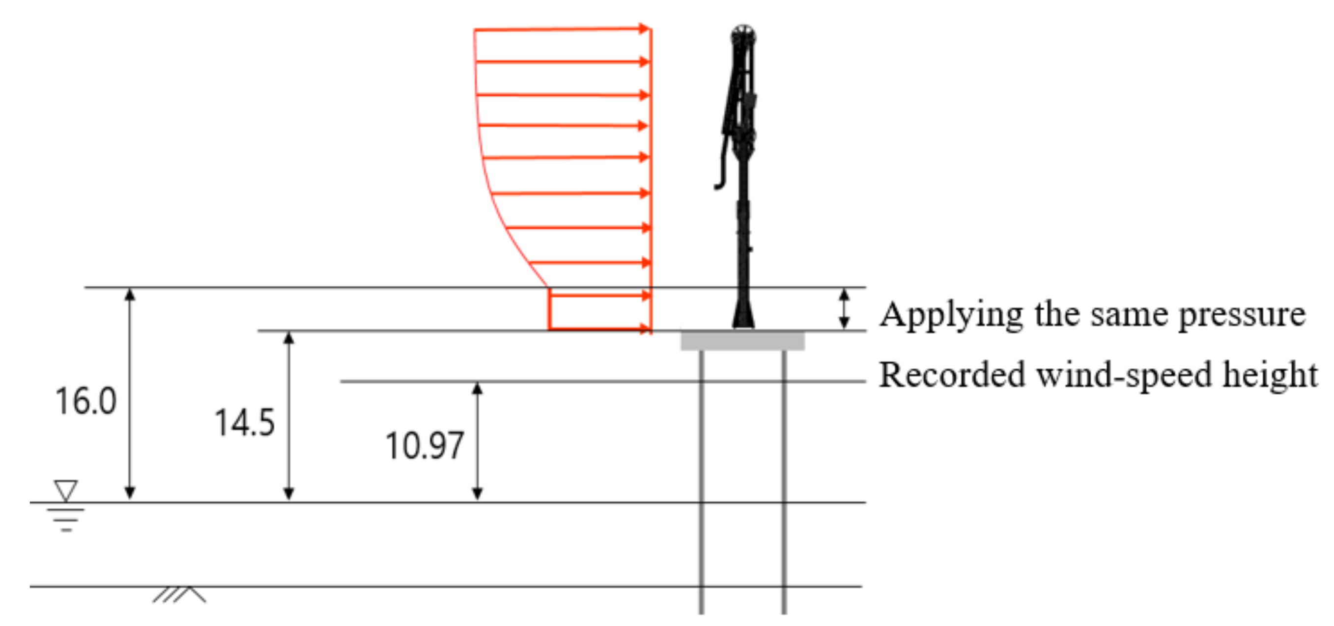
In this study, the foundations of the ULA system were located about 14.5 m above sea level (A.S.L.), as shown in Figure 6. Therefore, the main loads on these structures were the permanent load (self-weight) and the wind load. Due to the uncertainty of the wind speed of the harbor area, the model was established by statistical methods and considered the wind load as one of the random variables in the reliability analysis. The wind-speed data were collected in “A” harbor in Korea as described in Table 4. The data used in this study are the observation data produced by the Automatic Weather Station (AWS) at 10.97 m A.S.L. for 10 min interval from January 2001 to December 2020.
Wind speed increases with height and the expression for the variation in wind speed ( V ) with height ( h ) by the following equation bellow [24]:
V V 0 = h h 0 n
where V 0 is the mean wind speed recorded at height h 0 = 10.97 m A.S.L, V is the mean wind speed corresponding to the height h, and n is the power law exponent. Numerically, parameter n lies in the range 1/10–1.4. A typical value of n is assumed in most cases to be 1/7 [25]. However, for tower crane structures installed on the coast, an n value of 1/4 is recommended. The wind speed at the height of 16 m was applied for the structural components under 16 m.
Probability density functions are used to determine the wind potential in a specific area. There are several distributions used in modeling wind speed in the literature as Weibull, Log-normal, and Normal distributions. Given that fitting between the selected model and actual data is a question, several probability density functions should be compared to produce a minimum fitting error. In this study, the wind-speed data were expressed by the Weibull, Log-normal, and Normal distributions. Then, the Kolmogorov–Smirnov (K–S) and chi-square ( χ 2 ) tests were used to evaluate the performances of these distributions to find out the best fitting tool for the wind-speed data.
The two-parameter Weibull distribution is the most commonly used distribution in analyzing wind speed. The probability density function (PDF) and cumulative distribution function (CDF) of Weibull distribution are expressed as:
f X x = k b x b k 1 exp x b k
F X x = 1 exp x b k
where x is the wind speed, and k and b are the shape and scale parameters, respectively. The Log-normal distribution is also represented by two parameters: ζ X is the scale parameter and λ X is the shape or location parameter. The PDF and CDF for Log-normal distribution are as follows:
f X x = 1 2 π ζ X x exp 1 2 ln x λ X ζ X 2
F X x = Φ ln x λ X ζ X 2
The Normal PDF f X x and its CDF F x are expressed, respectively, by the following formulae with the mean and standard deviation of μ X and σ X :
f X x = 1 σ X 2 π exp 1 2 x μ X σ X 2
F X x = x 1 σ X 2 π exp 1 2 x μ X σ X 2 d x
Characteristics of these distributions calculated analytically from the available data are presented in Table 5. 
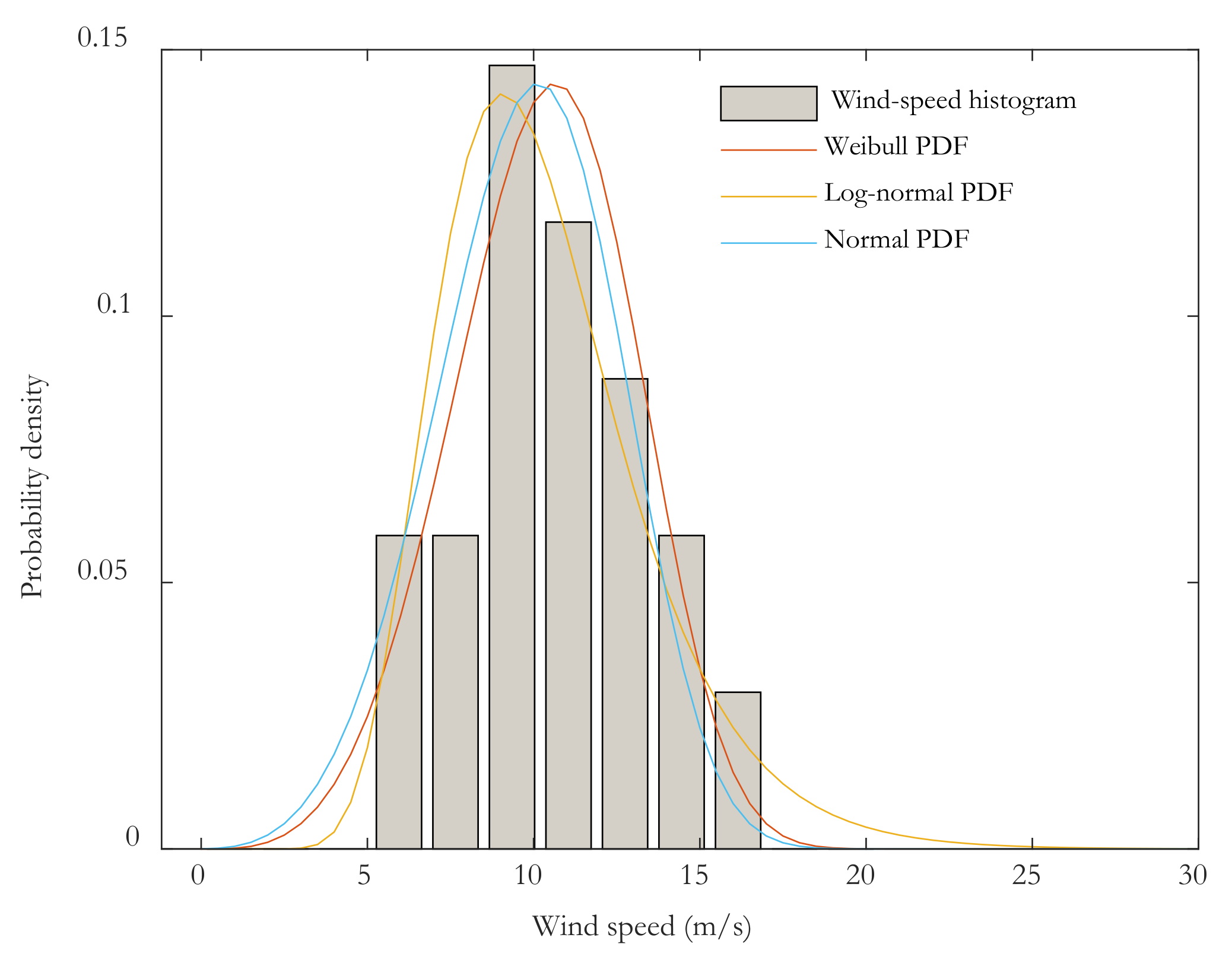
Figure 7 is the comparison of PDFs of actual and theoretical distributions. PDFs of all applied distributions are shown by different line types over the actual distribution represented in the form of a histogram. It can be observed from the naked eyes that peak densities of Weibull, Log-normal, and Normal distributions seem in line but are not in line with the peak density of the actual distribution. These qualitative comparisons also show that each PDF follows the form of a histogram, and the fitting of the two models Weibull and Normal is somewhat close. The selected distribution will be concluded based on the comparison results of goodness-of-fit statistics tests among three statistical distributions.
The K–S test gives absolute deviations between the actual distribution function ( S n ) and the specified theoretical CDF ( F X ). The empirical CDF for actual wind-speed data can be calculated by Equation (16) and the K–S statistics can be calculated by using Equation (17). The χ 2 test can be represented mathematically by Equation (18) [26]. The χ 2 value can be called as the overall error of probability distribution. Therefore, the lower the value of χ 2 , the more accurate the model results will be.
S n x i = 1 N n i
where N is the size of x i range, and n i is the number of points smaller than x i .
KS = S n F X
χ 2 = v i e i 2 e i
where v i and e i are the observed and theoretical frequency in the ith class interval, respectively.
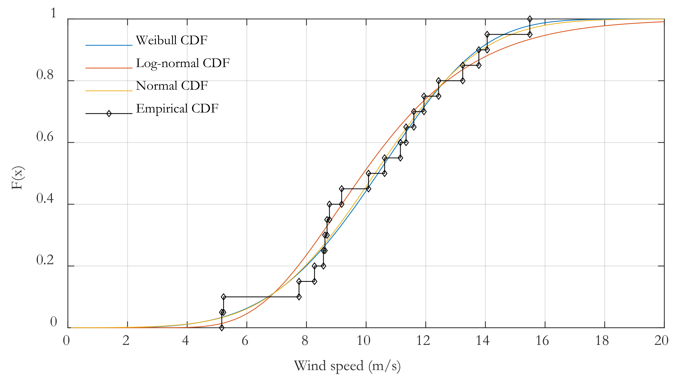
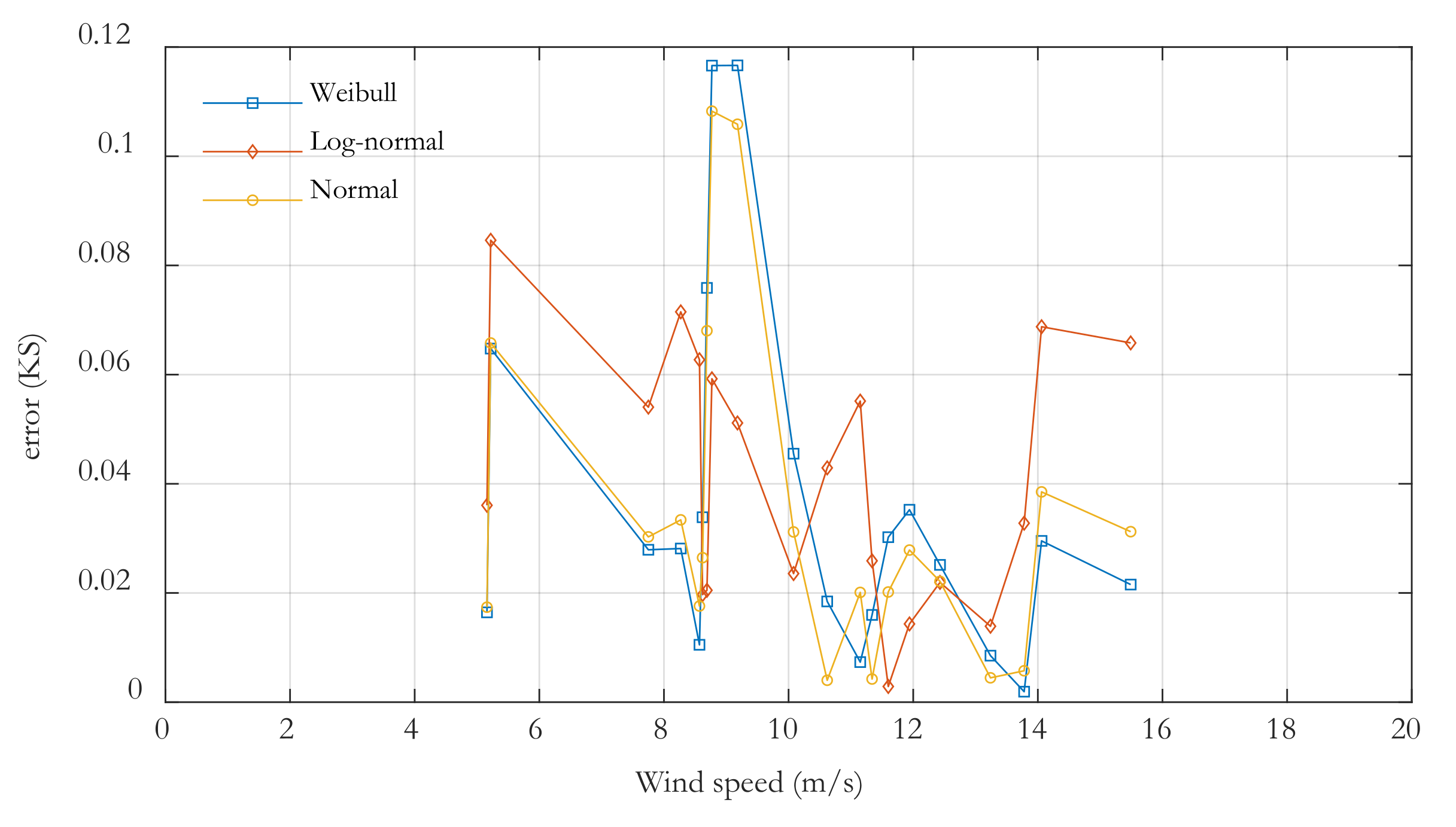
Figure 8 presents CDFs of the three distributions. The difference between the observation and estimation values can be seen clearly. From Figure 8, the error between the empirical CDF and theoretical CDF was obtained and shown in Figure 9. Table 6 includes the K–S test and χ 2 test values of applied distributions. Bold values indicate the best results. The results reported in Table 6 indicated that, based on the results of the K–S test, log-normal distribution was found to be the best one followed by Weibull and Normal distribution. The Weibull distribution showed better performance compared with others based on the statistics value of the χ 2 test. In this study, as a conclusion, the Log-normal distribution was chosen for the wind-speed random variable in the reliability analysis because it provides a better modeling in terms of the K–S criteria.

3.4. System Reliability in View of the NDT

The reliability analysis of the existing ULA system (36 age structural system) subjected to wind action is now performed. The limit-state function, Equation (1), for stress failure of the particular structural component can be written as:
g X 36 = S y , 36 S max ,   36 T , E , V
where S y , 36 and S max ,   36 are the yield stress and the maximum stress at time t = 36 years. T and E are the member thickness and the elastic modulus, respectively. The yield stress S y ,   36 was defined as a random variable of which characteristic values are described in Table 7. Table 8 summarizes stochastic model assumptions of the random variables considered in the reliability analysis related to the assessment of the ultimate stress of the structural components. The notation “various” means that the value depends on the structural component being considered. Both member thickness and elastic modulus are assumed to follow a normal distribution [27,28]. Accordingly, the bias factor for thickness is taken as 1.05 with a coefficient of variation (COV) of 4.4%, whereas the bias and COV for elastic modulus are taken as 0.987 and 7.6%, respectively. The yield stress distribution is assumed as the log-normal distribution where the bias factor and COV are 1.11 and 6.8%, respectively. The distribution of wind speed was discussed in Section 3.3. Under the action of wind and self-weight, the maximum response of each structural component in terms of stress was obtained and analyzed.
The reliability index is a parameter that provides a measure of structural safety. As presented in Section 2, in this study, the RSM (Response Surface Method)-based FORM was used to calculate the reliability indices. The basic methodology in the form of a detailed flowchart can be summarized as shown in Figure 10. Most of the reliability index simulations converged after three iterations.
Table 9 and Table 10 are the reliability indices and failure probability results, respectively, for five major structural components, namely, riser, base plate, anchor bolts, and inner and outer arm supports, corresponding to each model of the ULA. 
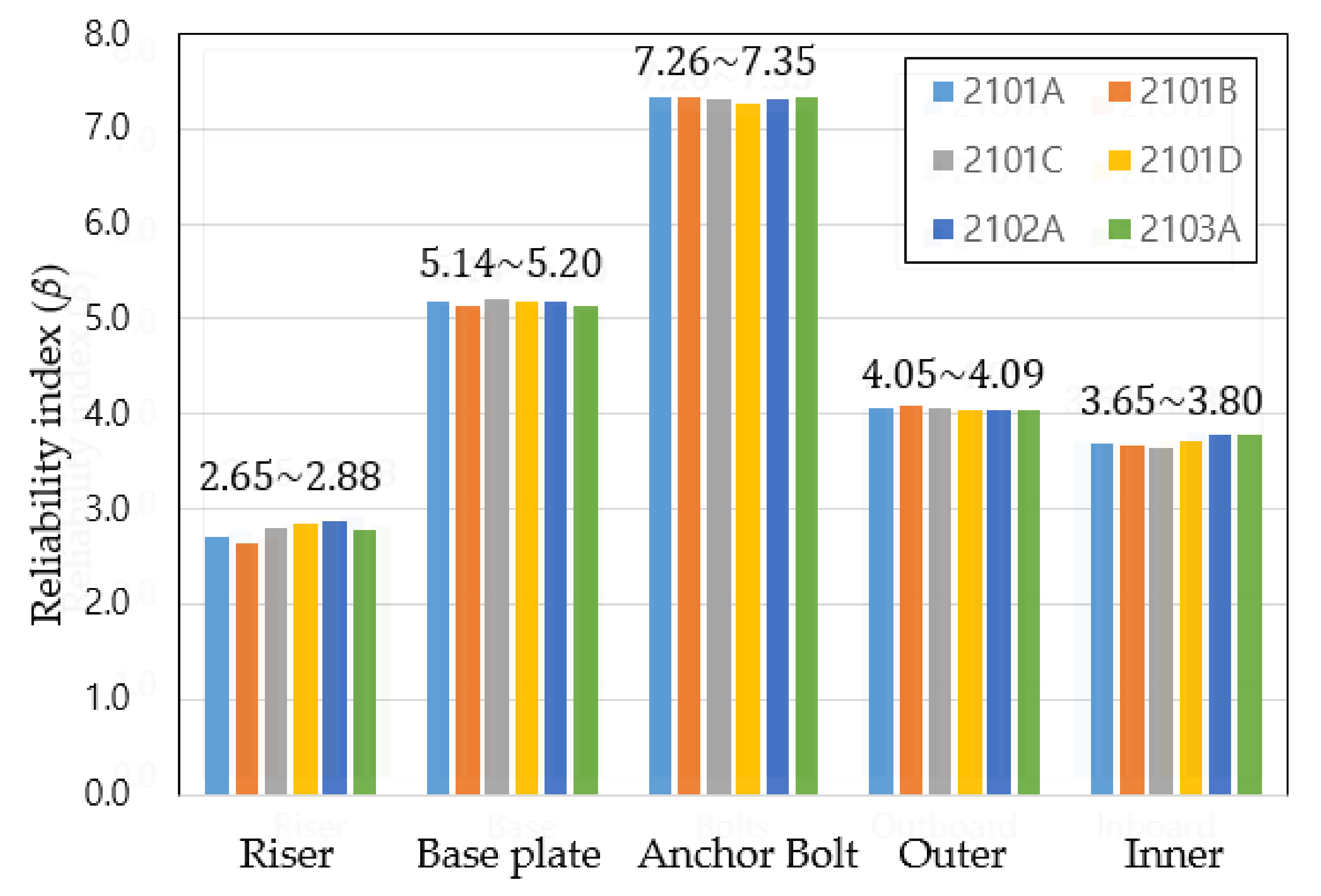
Figure 11 summarizes the reliability indices of ULAs classified by components. From Table 9 and Figure 11, it can be seen that the minimum reliability index corresponds to the riser component, which accounts for the damage caused by wind phenomena. Risers with the function of connecting the upper structure to the ground, bearing the entire weight, were particularly vulnerable. For the six ULA models, reliability ranges were 2.465–2.882 for risers, 5.136–5.203 for baseplates, 7.262–7.346 for anchor bolts, 4.049–4.088 for external arm supports, and 3.654 to 3.796 for internal arm supports, respectively. Obviously, the reliability indices depended on the particular component being considered. However, in general, the reliability indices corresponding to each ULA model increase in the order of riser, inner arm support, outer arm support, base plate, and anchor bolt. Anchor bolts have the highest reliability indices followed by the base plate, which implies that these two components are less vulnerable to wind action. This is because these two components are located on the foundation surface, convenient for maintenance and periodic inspection. In the evaluation, the deterioration state of structural components was considered in consideration of inspection data by an NDT, but the anchor bolt and base plate components were not deteriorated due to good maintenance such as early replacement. Their reliability index can here be seen as the original or design reliability index. Comparing the reliability index target with the results in 
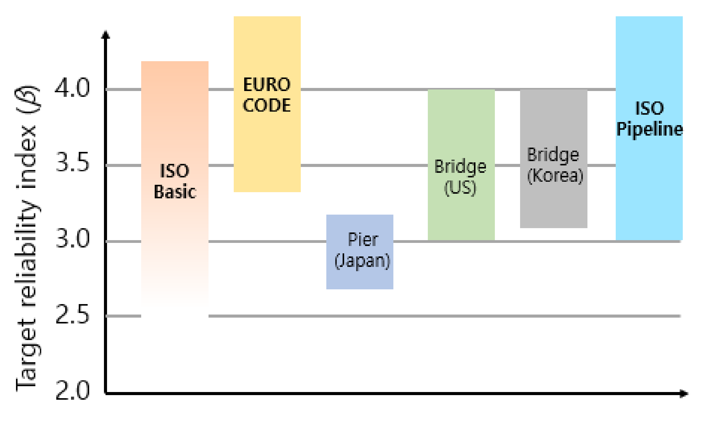
Table 9, it can be concluded that, presently, all structural components are safe since their reliability values are higher than the target reliability index value (2.6). Some evaluations were also similarly given in terms of failure probability. The failure probability of the riser was the highest and the lowest for the anchor bolt component. In general, the failure probabilities of the entire ULA system are low, within the safe range ( < 4.66 × 10 3 ) .
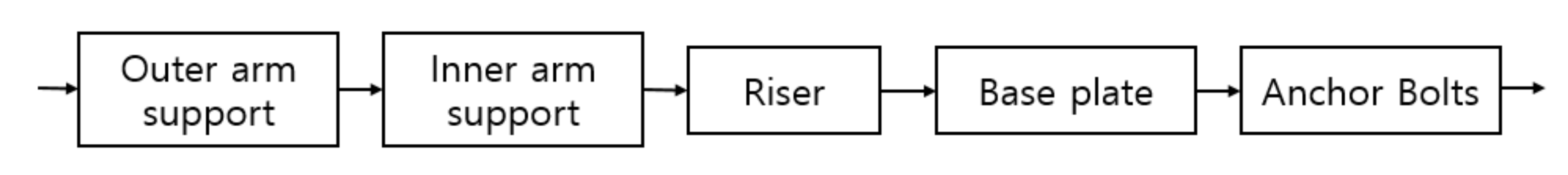
It can be seen that the normal operation of ULAs is possible only when all structural members are not damaged. Thus, each individual ULC can be considered as a distributed system of its components, as illustrated in Figure 12. Hence, the failure probability of each ULA can be determined as in Equation (9), in which P f , i is the failure probability of each component (see Table 10). In this study, only failure probability of five main structural components (including riser, base plate, anchor bolt, and outer and inner arm support) was considered, so the overall failure probability of each ULA model can be considered to be calculated from the failure probability of the five components. The results are shown in 
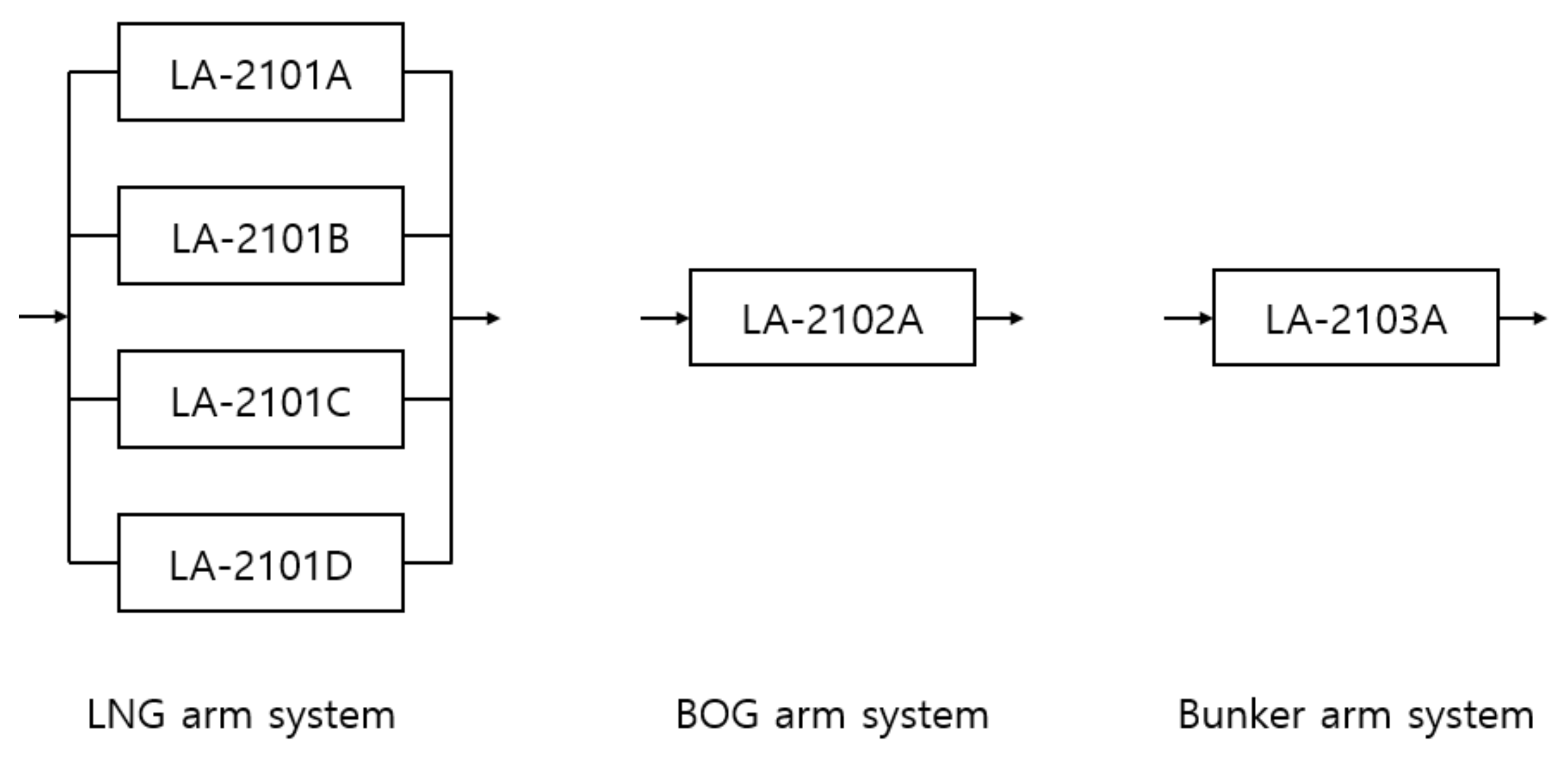
Table 11. As seen, the highest and lowest failure probabilities corresponded to the 2101B model of the LNG arm system and 2102A model of the BOG arm system. On the other hand, it can be seen that the failure probability of the models in the LNG arm system is different even though they are all of the same model type, are installed in the same location, and perform the same functions. This difference is the result of the difference in corrosion loss from location to location even if they experienced the same corrosion environment and time. This leads to the conclusion that assessing the reliability of port infrastructures should be implemented case-by-case. The four LNG arms (LA-2101A to LA-2101D) operate on the same system and perform the same functions. However, if one of them fails, the remaining ULAs in the system still function, so they can be seen as functionally parallel systems.
Since this LNG arm system loses its function if all four ULAs in the system fail at the same time, the failure probability of this LNG arm system can be calculated by Equation (8), where P f , U L A i is the failure probability of ULA models in the same system (see Table 11). The BOG arm (BOG) and Bunker arm (B/C) systems consist of only one unloading arm, as in Figure 13, so the failure probability of the ULA is the same as the failure probability of systems. The results of failure probability and corresponding reliability index of systems are given in Table 12. It can be seen that the failure probability of the LNG arm system is very low. This can be explained in that four ULA models failing at the same time is extremely rare.

3.5. Time-Dependent Reliability of Riser

As an example of the application of reliability in practical engineering, in this section, the most vulnerable structural component of each ULA model is analyzed based on the proposed time-dependent reliability analysis process. The riser has been shown to be the most vulnerable component to environmental deterioration and wind action, and it has the lowest reliability index compared with other components, in the range of 2.645–2.882 (see Table 9). Accordingly, the change in the reliability index of the riser over time was investigated, and analysis was performed until the reliability index reached the target reliability index limit (2.6).
As discussed before, the deterioration of structures will lead to degradation of resistance and an increased load effect. In this study, only the mean value of the member thickness variable is considered as a mean time-dependent resistance. With other factors such as yield stress and elastic modulus, their mean values are assumed to be constant over time. In the coastal marine environment, corrosion caused by oxidation is a major concern affecting the durability of steel structures. This study assumed that general corrosion occurs in the entire outer shell. In practice, corrosion is a stochastic process managed by many variables such as location, maintenance, environmental condition, etc. Therefore, only probabilistic models can describe the thickness loss. For this reason, the remaining thickness member of structural components was assumed to follow a normal distribution with two parameters: bias and COV are 1.05 and 0.044, respectively. The mean value of the remaining thickness member at any time can be derived from the bi-logarithmic model, which is typically used to describe the general corrosion of materials, as follows:
T t = T 0 C t
where C t = A t B is the corrosion loss as a function of time and is presented in Section 2.3. Accordingly, B = 0.69 was assumed and A is the corrosion loss in the first year. With aging structures, and missing or lost recorded data, this coefficient determination is difficult and usually assumed or obtained from laboratory observations. However, this method is still of limited usefulness. This study proposes to use NDT data to determine this parameter. The results are shown in Table 13. Note that, in the Table, T0 is the initial thickness member, and 
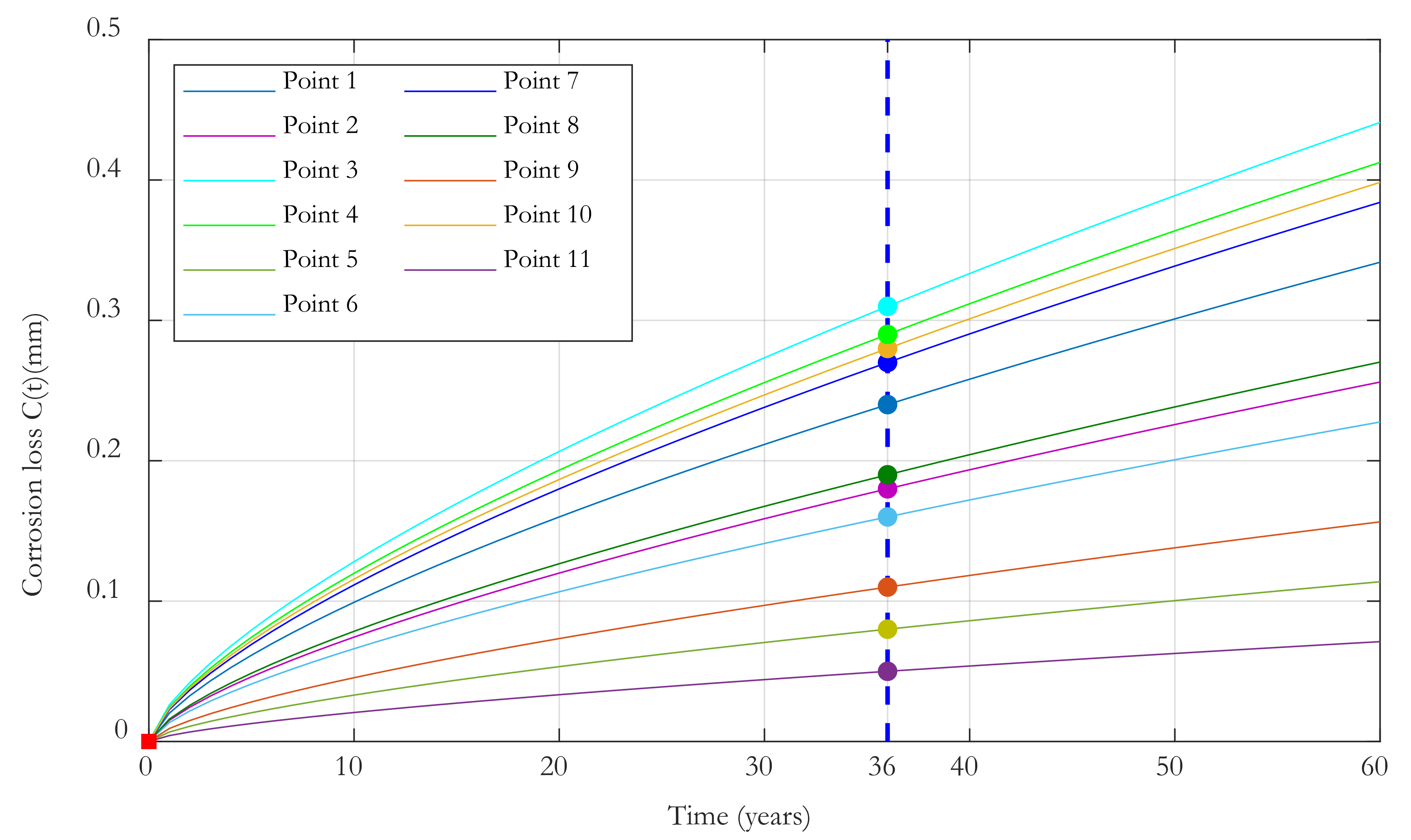
T(36) is the result of an NDT. With the obtained coefficients A and B, the relationship between corrosion loss (mean corrosion depth) and exposure period is illustrated in Figure 14 where the value denoted by the square is the initial corrosion loss (=0) and the values denoted by the circle are the measured corrosion loss at the time of assessment C(36).
It is evident from Figure 14 that the corrosion loss increased with the exposure period, but the loss rate became slower. This could be the effect of protective measures such as anti-corrosion paint, routine maintenance, etc. This means that, if a more effective protection level of a steel pipe is provided, then a lower rate of corrosion may be obtained.
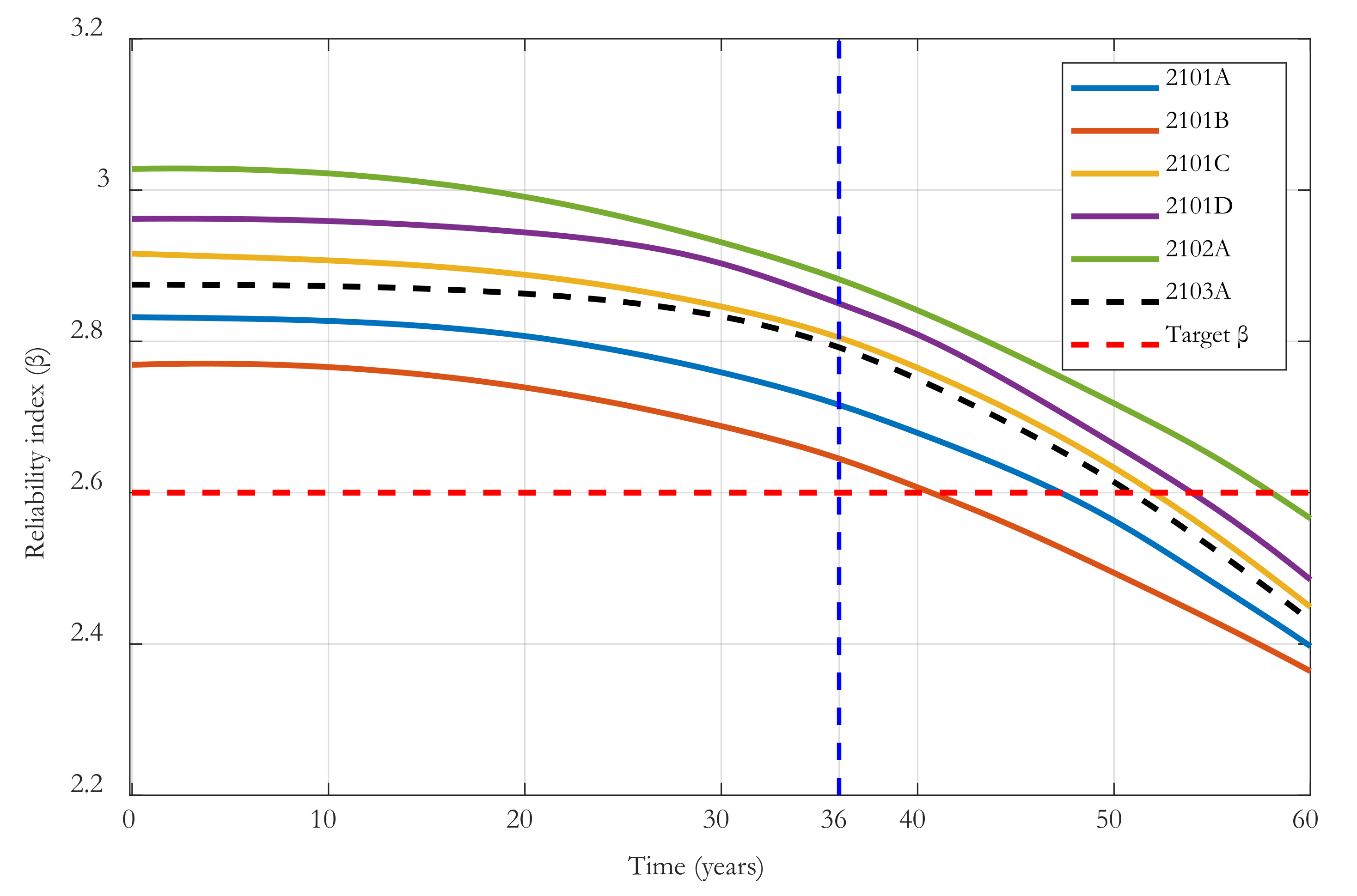
The results are presented in Table 14 and Figure 15. As illustrated in Table 14 and Figure 15, one can see how the reliability index of the initial structure changes over time under the effect of degradation. General corrosion is considered as the major factor leading to the deterioration of the structure. These reliability index curves can be divided into three phases: the current reliability index (36 age), the past reliability index (before 36 age), and the future reliability index (after 36 age). Furthermore, if the current protective measures and routine maintenance are maintained, when the target reliability index was assumed to be 2.6, the riser had around a 40.7-year lifetime for the 2101B model, and 47.3, 52, 54, 58, and 50.9-year lifetimes for 2101A, 2101C, 2101D, 2102A, and 2103A models, respectively. The corresponding remaining service life (RSL) is also summarized in Table 15. This result provides quantitative prediction useful for planning maintenance or replacement to increase structural service life.

4. Conclusions

The paper has described the process and models used for reliability analysis of the aging ULA systems in the harsh marine environment. Both the load effect (stress) and the acceptable limit (yield stress) were modeled based on stochastic processes to consider deterioration. In particular, an appropriate probabilistic model that describes the loss of material due to corrosion was proposed by combining the bi-logarithmic model   C t = A t B , typically used to describe corrosion loss as a function of time, with NDT data. This method is relatively simple but still provides reliable results. The results from the reliability index analysis of the individual components of the existing ULA system indicated that, presently, all structural components are safe since their reliability values are above the target reliability index. On the other hand, a process was also established to evaluate the failure probability of a system based on the correlation between components in the same system. In addition, the results from the time-dependent reliability index analysis provided a quantitative prediction of the maximum remaining service time of the most vulnerable component. This prediction is useful for repair and replacement planning and infrastructure management. By this approach, the remaining service time of other components or other aging infrastructure is conveniently obtained.

Author Contributions

Conceptualization, D.-V.N. and D.-H.K.; methodology, D.-V.N. and D.-H.K.; software, D.-V.N.; validation, D.-H.K.; formal analysis, D.-V.N. and J.-K.L.; data curation, D.-V.N. and J.-K.L.; writing—original draft preparation, D.-V.N.; writing—review and editing, D.-V.N. and D.-H.K.; supervision, D.-H.K. All authors have read and agreed to the published version of the manuscript.

Funding

This research received no external funding.

Data Availability Statement

Not applicable.

Conflicts of Interest

The authors declare no conflict of interest.

References

  1. Melchers, R.E. The effect of corrosion on the structural reliability of steel offshore structures. Corros. Sci. 2005, 47, 2391–2410. [Google Scholar] [CrossRef]
  2. Wang, C.; Zhang, H.; Li, Q. Reliability assessment of aging structures subjected to gradual and shock deteriorations. Reliab. Eng. Syst. Saf. 2017, 161, 78–86. [Google Scholar] [CrossRef]
  3. Ciampoli, M. Time dependent reliability of structural systems subject to deterioration. Comput. Struct. 1998, 67, 29–35. [Google Scholar] [CrossRef]
  4. Vu, T.K.A.; Mark, G.S. Structural reliability of concrete bridges including improved chloride-induced corrosion models. Struct. Saf. 2000, 22, 313–333. [Google Scholar] [CrossRef]
  5. Mark, G.S.; John, A.M. Spatial time-dependent reliability analysis of corrosion damage and the timing of first repair for RC structures. Eng. Struct. 2007, 29, 1457–1464. [Google Scholar] [CrossRef]
  6. Li, Q.; Wang, C. Updating the assessment of resistance and reliability of existing aging bridges with prior service loads. J. Struct. Eng. ASCE 2015, 141, 04015072. [Google Scholar] [CrossRef]
  7. Wang, C.; Michael, B.; Bilal, M.A. Time-dependent reliability of aging structures: Overview of assessment method. J. Risk Uncertain. Eng. Syst. 2021, 7, 3121003. [Google Scholar] [CrossRef]
  8. Frangopo, D.; Dong, Y.; Sabatino, S. Bridge life-cycle performance and cost: Analysis, prediction, optimisation and decision-making. Struct. Infrastruct. Eng. 2017, 13, 1239–1257. [Google Scholar] [CrossRef]
  9. Akiyama, M.; Dan, M.F.; Hiroki, I. Toward life-cycle reliability-, risk- and resilience-based design and assessment of bridges and bridge networks under independent and interacting hazards: Emphasis on earthquake, tsunami and corrosion. Struct. Infrastruct. Eng. 2019, 16, 26–50. [Google Scholar] [CrossRef]
  10. Mori, Y.; Ellingwood, B.R. Reliability-based service-life as assessment of aging concrete structures. J. Struct. Eng. ASCE 1993, 119, 1600–1621. [Google Scholar] [CrossRef]
  11. Michael, P.E.; Dan, M.F. Service-life prediction of deteriorating concrete bridges. J. Struct. Eng. 1998, 124, 309–317. [Google Scholar]
  12. Mussini, R.; Cancela, H.; Clarke, T. Structural reliability assessment of cracked pipes: The role of probability of detection data. Fatigue Fract. Eng. Mater. Struct. 2019, 42, 664–673. [Google Scholar] [CrossRef]
  13. Bhargava, K.; Mori, Y.; Ghosh, A.K. Time-dependent reliability of corrosion-affected RC beams. Part 2: Estimation of time-dependent failure probability. Nucl. Eng. Des. 2011, 241, 1385–1394. [Google Scholar] [CrossRef]
  14. Liu, Y.; Dan, M.F. Time-dependent reliability assessment of ship structures under progressive and shock deteriorations. Reliab. Eng. Syst. Saf. 2018, 173, 116–128. [Google Scholar] [CrossRef]
  15. Sajedi, S.; Huang, Q. Reliability-based life-cycle-cost comparison of different corrosion management strategies. Eng. Struct. 2019, 186, 52–63. [Google Scholar] [CrossRef]
  16. Haldar, A.; Mahadevan, S. Reliability Assessment Using Stochastic Finite Element Analysis; John Wiley & Sons: New York, NY, USA, 2000; pp. 56–60. [Google Scholar]
  17. Murray, R. Remarks on a multivariate transformation. Ann. Math. Stat. 1952, 23, 470–472. [Google Scholar]
  18. Gerhart, I.S.; Christian, G.B.; Ulrich, B.; Winai, O. On efficient computational schemes to calculate structural failure probabilities. Probabilistic Eng. Mech. 1989, 4, 10–18. [Google Scholar] [CrossRef]
  19. Kim, D.-H.; Lee, S.-G. Reliability analysis of offshore wind turbine support structures under extreme ocean environmental loads. Renew. Energy 2015, 79, 161–166. [Google Scholar] [CrossRef]
  20. Feliu, S.; Morcillo, M.; Feliu, S. The prediction of atmospheric corrosion from meteorological and pollution parameters—II. Long-term forecasts. Corros. Sci. 1993, 34, 415–422. [Google Scholar] [CrossRef]
  21. EN 1990; Eurocode Basis of Structural Design. European Committee for Standardization (CEN): Brussels, Belgium, 2002.
  22. ISO 2394; General Principles on Reliability for Structures. International Organization for Standardization: Geneve, Switzerland, 2015.
  23. Sotberg, T.; Moan, T.; Bruschi, R.; Jiao, G.; Mork, K.J. The super B project: Recommended target safety levels for limit state based design of offshore pipelines. In Proceedings of the 16th International Conference on Offshore Mechanics and Arctic Engineering, Yokohama, Japan, 13–18 April 1997. [Google Scholar]
  24. James, F.M.; Jon, G.M.; Anthony, L.R. Wind Energy Explained: Theory, Design and Application; Wiley: New York, NY, USA, 2002. [Google Scholar]
  25. Sunday, O.O.; Muyiwa, S.A.; Samuel, S.P. Analysis of wind speed data and wind energy potential in three selected locations in south-east Nigeria. Int. J. Energy Environ. Eng. 2012, 3, 7. [Google Scholar] [CrossRef] [Green Version]
  26. Eugene, C.M.; Matthew, L.; Richard, M.V.; Laurie, G.B. Probability distributions for offshore wind speeds. Energy Convers. Manag. 2011, 52, 15–26. [Google Scholar] [CrossRef]
  27. Sonja, K.; Jasmina, M.; Goran, S.; Djordje, V.; Branko, T. Uncertainty in the determination of elastic modulus by tensile testing. Eng. Sci. Technol. Int. J. 2022, 25, 100998. [Google Scholar] [CrossRef]
  28. Paul, E.H.; Daniel, B.; Ibrahim, A.A.; Bilal, M.A. Uncertainties in material and geometric strength and load variables. Nav. Eng. J. 2002, 114, 139–166. [Google Scholar] [CrossRef]
Figure 1. Stochastic process of load effect S t and the deteriorating structural resistance R t .
Energies 15 09408 g001
Figure 2. The target reliability indices corresponding to several reference rules.
Energies 15 09408 g002
Figure 3. (a) Six models of the ULA system located at the “A” LNG terminal and (b) image of disassembling ULA components during a major restoration.
Energies 15 09408 g003
Figure 4. Finite-element model with main components of a typical unloading arm of this study.
Energies 15 09408 g004
Figure 5. (a) Sample points of the NDT used to define the deterioration function of structure over time and (b) thickness-inspection positions of each section in the NDT.
Energies 15 09408 g005
Figure 6. Schematic of the loads on the ULA system.
Energies 15 09408 g006
Figure 7. PDF comparison of all distributions.
Energies 15 09408 g007
Figure 8. Comparison of CDFs.
Energies 15 09408 g008
Figure 9. The relative error of CDFs between the applied distributions and actual distribution.
Energies 15 09408 g009
Figure 10. Flowchart for reliability analysis of an unloading arm.
Energies 15 09408 g010
Figure 11. Summary of the reliability index of ULAs classified by components.
Energies 15 09408 g011
Figure 12. The distributed system of ULA Components.
Energies 15 09408 g012
Figure 13. The parallel system of ULAs.
Energies 15 09408 g013
Figure 14. Time-dependent corrosion loss.
Energies 15 09408 g014
Figure 15. Reliability index as a function of time.
Energies 15 09408 g015
Table 1. Failure probability level.
Safety Classes
Limit StatesLowNormalHigh
SLS10−1–10−210−2–10−310−2–10−3
ULS10−2–10−310−3–10−410−4–10−5
FLS10−310−410−5
ALS10−410−510−6
Table 2. Six models of the ULA system.
SystemModelMass (Metric Ton)
LNG arm (L)2101A, 2101B, 2101C, 2101D52.000
BOG arm (BOG)2102A52.000
Bunker arm (B/C)2103A49.000
Table 3. Measured thickness from the NDT at sample points (unit: mm).
ComponentPoint2101A2101B2101C2101D2102A2103A
Riser112.7613.2913.3514.4213.4213.57
212.8212.4213.2213.4113.6513.15
321.6921.321.716.4522.1120.45
414.2113.313.4419.6313.212.82
Outer arm support512.9212.4812.5113.412.8912.64
613.3413.5812.9613.0813.3613.26
79.739.539.249.8410.3110.22
812.3112.8812.4513.2713.3412.76
Inner arm support99.3911.799.509.119.069.24
1014.7214.3814.9914.3715.0214.89
119.959.829.669.939.139.60
Table 4. Wind-speed data at “A” harbor.
YearWind Speed,
10 Min Mean (m/s)
YearWind Speed,
10 Min Mean (m/s)
20015.1620119.18
200210.62201211.94
20035.2220137.75
200410.08201411.15
20058.7720158.57
200611.34201615.49
200711.620178.27
20088.69201812.43
20098.62201913.24
201014.06202013.78
Table 5. Characteristics of distributions.
DistributionWeibullLog-NormalNormal
Parametersk = 11.326 λ X = 2.293 μ X = 10.298
b = 4.296 ζ X = 0.297 σ X = 2.278
Table 6. Comparison of three distributions in terms of goodness-of fit test indicators.
TestWeibullLog-normalNormal
K–S0.1080.0850.117
χ 2 2.033.972.13
Table 7. Design value of yield stress.
ComponentMaterial CodeYield Stress, S y (MPa)
RiserASTM A516 G60220
Base plateASTM A312 TP304L170
Anchor boltsASTM A312 TP304L170
Outer arm supportASTM A516 G60220
Inner arm supportISO 898-1 8.8640
Table 8. Probabilistic models of the random variables used in the reliability analysis.
Random VariableDistribution ParametersType of Distribution
MeanBias FactorCOV
T (Thickness, mm)Various1.050.044Normal
E (Elasticity Modulus, GPa)2000.9870.076Normal
V (Wind speed, m/s) λ X = 2.293, ζ X = 0.297, see Table 5Log-normal
S y (Yield stress, MPa)Various1.110.068Log-normal
Table 9. Reliability index results of structural components.
Component2101A2101B2101C2102A2101D2103A
Riser2.7162.6452.8052.852.8822.792
Base plate5.1945.1365.2035.1895.1935.147
Anchor bolts7.3247.3387.3017.2627.3177.346
Outer arm support4.0554.0884.0574.0494.054.053
Inner arm support3.6943.6743.6543.7053.7963.778
Table 10. Probability failure results of structural components.
Component2101A2101B2101C2102A2101D2103A
Riser3.30 × 10−34.09 × 10−32.52 × 10−32.18 × 10−31.98 × 10−32.62 × 10⁻³
Base plate1.03 × 10−71.41 × 10−79.83 × 10−71.06 × 10−71.04 × 10−71.32 × 10⁻⁷
Anchor bolts1.21 × 10−131.08 × 10−131.43 × 10−131.91 × 10−131.27 × 10−131.03 × 10⁻¹³
Outer arm support2.51 × 10−52.18 × 10−52.49 × 10−52.57 × 10−52.56 × 10−52.52 × 10⁻⁵
Inner arm support1.10 × 10−41.19 × 10−41.29 × 10−41.06 × 10−47.36 × 10−47.91 × 10⁻⁴
Table 11. Failure probability and corresponding reliability index of the ULA models.
SystemModel P f β
LNG arm (L)2101A3.436 × 10−32.703
2101B4.228 × 10−32.633
2101C2.673 × 10−32.785
2101D2.314 × 10−32.832
BOG arm (BOG)2102A2.077 × 10−32.866
Bunker arm (B/C)2103A2.723 × 10−32.779
Table 12. Failure probability and corresponding reliability index of the ULA systems.
System P f β
LNG arm (L)8.984 × 10−116.378
BOG arm (BOG)2.077 × 10−32.866
Bunker arm (B/C)2.723 × 10−32.779
Table 13. Determining the A parameter.
ComponentsPointT0T(36)C(36)BA
Riser11312.760.240.690.0202
21312.820.180.0152
32221.690.310.0262
414.514.210.290.0245
Outer arm support51312.920.080.0067
613.513.340.160.0135
7109.730.270.0228
812.512.310.190.016
Inner arm support99.59.390.110.0093
101514.720.280.0236
11109.950.050.0042
Table 14. Reliability analysis results.
Time (Year)2101A2101B2101C2101D2102A2103A
02.8322.7692.9162.9623.0282.875
102.8272.7662.9072.9593.0222.873
202.8072.7392.8882.9442.9912.863
302.7592.6882.8462.9032.9312.833
362.7162.6452.8052.8502.8822.792
402.6792.6072.7652.8092.8412.750
452.6272.5542.7052.7412.7822.687
502.5632.4942.6332.6642.7182.614
552.4822.4312.5472.5822.6492.527
602.3972.3642.4492.4852.5662.431
Table 15. Predicted remaining service life of Riser based on the assumption of target β of 2.6.
ULA Model2101A2101B2101C2101D2102A2103A
RSL (years)11.34.716.018.022.014.9
Publisher’s Note: MDPI stays neutral with regard to jurisdictional claims in published maps and institutional affiliations.

