Energy Disaggregation Using Multi-Objective Genetic Algorithm Designed Neural Networks

Abstract

Energy-saving schemes are nowadays a major worldwide concern. As the building sector is a major energy consumer, and hence greenhouse gas emitter, research in home energy management systems (HEMS) has increased substantially during the last years. One of the primary purposes of HEMS is monitoring electric consumption and disaggregating this consumption across different electric appliances. Non-intrusive load monitoring (NILM) enables this disaggregation without having to resort in the profusion of specific meters associated with each device. This paper proposes a low-complexity and low-cost NILM framework based on radial basis function neural networks designed by a multi-objective genetic algorithm (MOGA), with design data selected by an approximate convex hull algorithm. Results of the proposed framework on residential house data demonstrate the designed models’ ability to disaggregate the house devices with excellent performance, which was consistently better than using other machine learning algorithms, obtaining F1 values between 68% and 100% and estimation accuracy values ranging from 75% to 99%. The proposed NILM approach enabled us to identify the operation of electric appliances accounting for 66% of the total consumption and to recognize that 60% of the total consumption could be schedulable, allowing additional flexibility for the HEMS operation. Despite reducing the data sampling from one second to one minute, to allow for low-cost meters and the employment of low complexity models and to enable its real-time implementation without having to resort to specific hardware, the proposed technique presented an excellent ability to disaggregate the usage of devices.

1. Introduction

Since the start of the energy crisis, energy-saving problems have risen in popularity among the general public [1]. According to the study reported in [2], the global energy problem is driven by global population increase, rising demand, and continuous reliance on fossil fuels for production. Moreover, global energy consumption influences greenhouse gas emissions and, thus, climate change [3]. As a result of this situation, several governments have acted and set CO² emission reduction objectives. For instance, China, one of the world’s major consumers of fossil fuels and major CO² emitter [2], promised to reach peak CO₂ emissions and carbon neutrality by 2030 and 2060, respectively [4]. Likewise, the European Union (EU) made a significant effort to combat global warming by implementing a variety of strategic policies [5,6].

The building sector is a prominent energy consumer and greenhouse gas emitter. For instance, it accounts for 27.5% of the overall final energy use in EU [5]. Therefore, there is a pressing need to halt the rising trend in building energy consumption. Energy management through adequate saving energy mechanisms has been the focus in recent years as a key strategy for conserving energy [1].

Home energy management systems (HEMS) are an efficient way to minimize energy consumption in a home while preserving occupant comfort [7,8]. The development of an effective HEMS system requires the implementation of a process to identify and monitor the principal loads in the household [9], thus allowing the HEMS to efficiently control the operation of (some) electric devices [10]. It also enables consumers to have a better awareness of their electricity usage patterns, potentially leading to more energy-conscious behavior and decreasing operating and electrical costs for grid operators and end users [11].

One of the techniques for monitoring appliances is to install measuring devices or sensors for each load of interest. This is known as intrusive load monitoring (ILM) in the literature and can properly estimate the operating condition of devices [12,13,14]. However, some disadvantages limit its practical application, such as the difficulties of deploying and configuring many sensors, its high cost, and its intrusive nature, which raises privacy and security concerns [15]. Non-intrusive load monitoring (NILM), on the other hand, aims to estimate the energy consumption of individual devices from a single meter that monitors the aggregated demand across many appliances [10]. It is one of the most effective energy disaggregation approaches since it enables users to disaggregate the power consumption of specific appliances in the household while maintaining user privacy and using smart meters that are already installed at the house entrance [15].

George Hart pioneered the use of NILM in [16,17]. He presented NILM as a monitoring system for appliances in an electrical circuit that turns ON and OFF independently. He showed that devices generate unique power consumption signatures. Therefore, the NILM techniques enable the recognition of these signatures from the total aggregated power consumption.

NILM algorithms are often classified into event-based algorithms [16,17,18,19] that relate signal state changes to device state changes and eventless algorithms that estimate a global system state using statistical and machine learning approaches [20]. Event-based approaches seek to detect and classify ON/OFF events of electrical devices. In Hart’s approach, the ON/OFF events were used to detect the operation of specific appliances using the aggregated active and reactive powers. However, the technique struggled to identify certain types of appliances (multistate appliances, continuously variable consumer appliances, and permanent consumer devices).

Subsequently, several other techniques have been explored to solve the problem of energy disaggregation. Initially, researchers were drawn to the approaches of hidden Markov models (HMM) and their extensions [21,22,23,24,25,26,27]. However, as the number of target appliances increases, the complexity of HMM models and their extensions grow exponentially. Furthermore, difficulties with generalization and scalability were noted for these approaches, as well as a large sensitivity to current inference techniques for state estimation to local optima, thus limiting their applicability in the real world [13].

To tackle this NILM challenge, researchers have lately resorted to machine learning methods. Indeed, both supervised and unsupervised approaches have been explored to address the challenge of NILM. Support vector machines demonstrated good performance in [28,29,30,31]. K-nearest neighbors were explored in [32,33], decision tree in [34,35], k-means clustering in [36], and graph signal processing in [37,38]. More recently, deep learning approaches have prompted an upsurge in NILM research. The studies reported in [39,40] were among the first to use deep learning-based NILM. In [40], three deep learning models (long short-term memory, convolutional neural network, and autoencoders) were compared. The models were trained using a six-second low frequency sampling rate using only the active power as the input feature. They obtained better performance than the factorial HMM and combinatorial optimization state of the art models. In [41], the authors presented a bidirectional long short-term memory model based on a low frequency sampling rate. They combined several electrical features to create a multi-feature input. The model was evaluated on low frequency data from the public datasets UKDALE and ECO. An approach based on deep convolutional networks was proposed in [42]. They classified the states of devices using a feature space enriched by the introduction of a temporal pooling module. The authors tested their model using the UKDALE low frequency dataset and demonstrated good generalization properties. In [43], a hybrid deep learning architecture based on a convex hull data selection approach using low frequency power data for NILM was proposed. They selected the most informative vertices of the real convex hull using a random approximation algorithm, incorporating them in the training data. They showed that the proposed framework is effective and performs well compared to existing approaches.

However, deep learning approaches require a large amount of training data to achieve satisfactory results [44]. This poses a major challenge for NILM algorithms due to the scarcity of high-quality datasets, both in terms of duration and label quality [10,45,46]. Additionally, such methods gain greatly from a large number of trainable parameters, which requires a processing capacity that is neither inexpensive nor cheaply accessible in most circumstances [44]. A comprehensive literature review of NILM approaches, beyond the scope of this paper, can be found in [15].

The application of NILM techniques depends strongly on the sampling rate, which refers to the frequency at which the meter measures the data. The sampling rate defines the type of information that can be obtained from the electrical signals [47]. There are two basic approaches for collecting data [13,14,15]: low frequency sampling rate (1 Hz or less) and high frequency sampling rate (in the range of kHz).

The high sampling frequencies enable the use of fine-grained characteristics such as harmonics [48], voltage-current (V-I) trajectory [49], and wavelet coefficients [50,51] from steady-state and transient. Although these methods may lead to good results in terms of device identification accuracy, high sampling frequency data have the drawbacks of being both difficult to transfer and store and very expensive in terms of software and hardware specificity [14]. Moreover, the current smart meter infrastructure, which typically allows for low sampling rates of the range of a few seconds, is not generally compatible with high frequency data collection and, therefore, specific equipment is required [52,53].

Conversely, low frequency methods are the ideal option in NILM applications since they enable the use of commonly used smart meter resources without requiring extra hardware. In principle, low-frequency data-based approaches perform load disaggregation by identifying the combination of states that substantially reduce the uncertainty margin [53]. However, the complexity and computational time of these methods may significantly increase with the number of appliances. Additionally, NILM algorithms must fulfill a variety of criteria, including good precision in recognizing device usage and accurately estimating their power consumption, using low complex models and low-cost equipment [15,41].

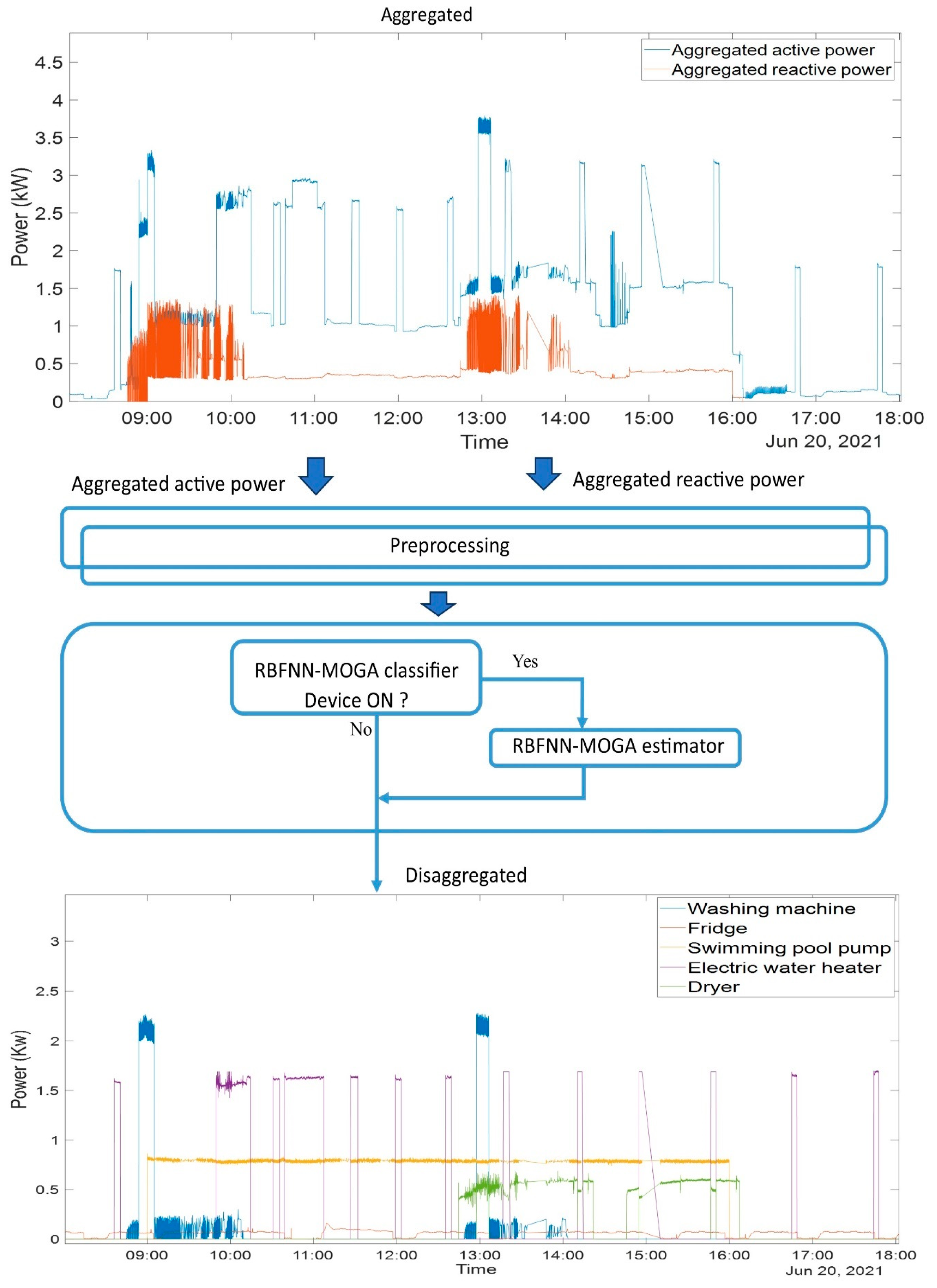
Therefore, there is the need to have an NILM technique available that, besides delivering very good results both in terms of operation detection and energy estimation, does not require specific acquisition systems, the existence of large amount of design data, and expensive processing power to design the classification and estimation models. To address these challenges, this paper proposes an NILM framework based on a low-frequency sampling rate, allowing the use of low-cost meters and employing low-complexity shallow neural network models. The following are the key contributions of this paper:

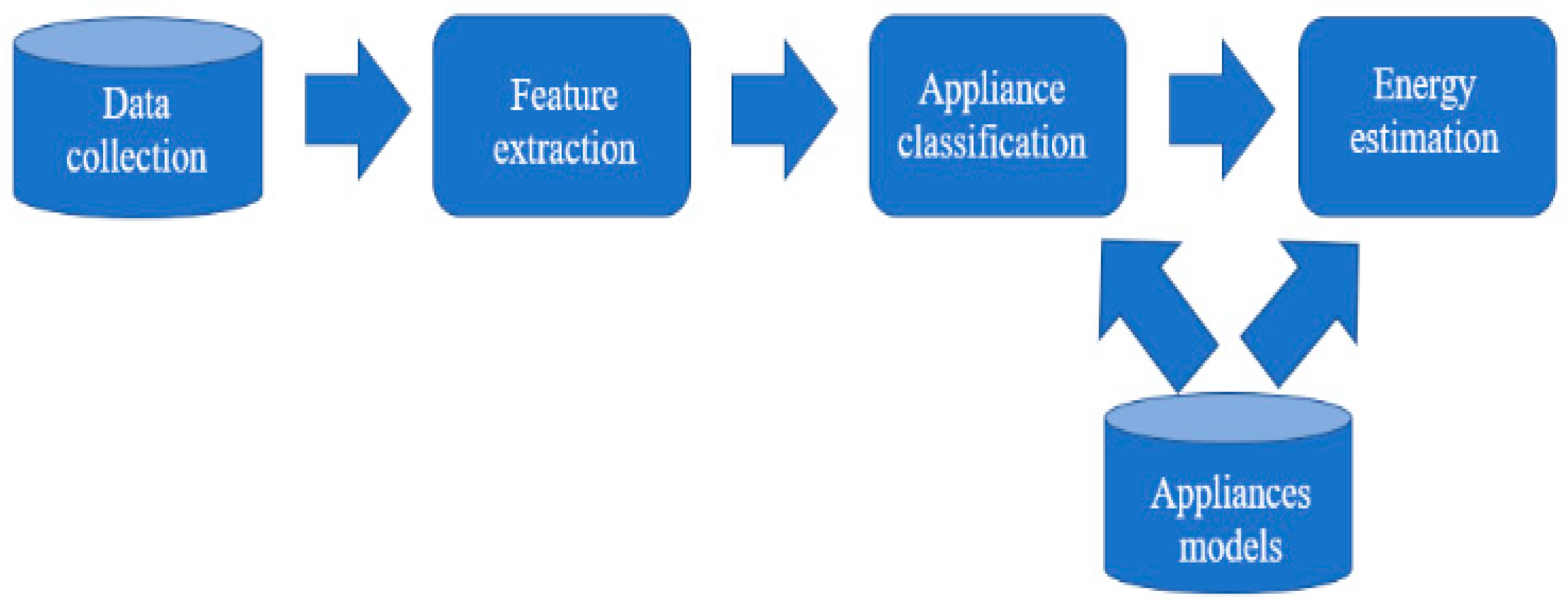
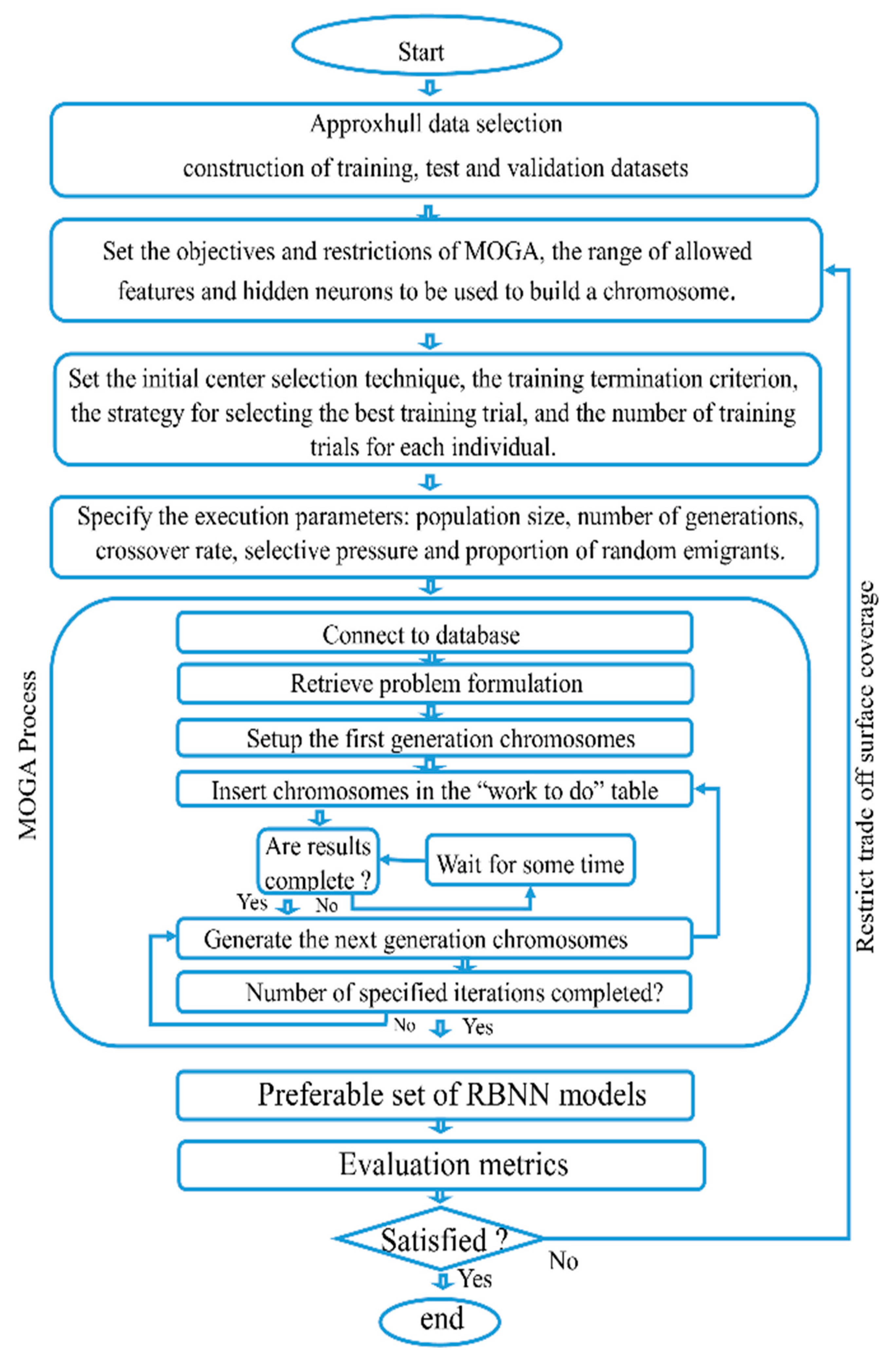
• A low-complexity NILM framework based on a radial basis function neural network designed by a multi-objective genetic algorithm (MOGA) with data selected by an approximate convex hull algorithm was proposed. The framework includes residential house data gathered in a real-life situation, feature extraction, appliance classification, and energy estimation.
• A comparative analysis of several computational intelligence’s classifiers for non-intrusive load monitoring using the same data, including support vector machine, k-nearest neighbors, decision trees, long short-term memory, and convolutional neural network, was performed.
• The feasibility of the approach was also validated using the public AMPds (Almanac of Minutely Power datasets) dataset, and a comparative study with other approaches was conducted.
• The proposed NILM framework was used to disaggregate one month of consumption of a case study house, identifying that 60% of the total consumption is related to schedulable devices, thus enabling a further degree of flexibility to HEMS.

The rest of the paper is structured as follows: Section 2 introduces the problem statement, the methods used, the data acquisition system, and the accuracy metrics employed. The obtained results are presented in Section 3, and their discussion is in Section 4. Section 5 concludes the paper.

2. Methodology

2.1. Problem Statement

The primary goal of NILM is to estimate the energy consumption of each individual device using aggregate data from the household’s total energy usage. Let x = [$x_1$, $x_2$, …, $x_T$] be a sequence of aggregated readings from a smart meter in the house. The aim is to estimate the contribution of each device $y^{\left(n\right)}$ = [$y_1^{\left(n\right)}$, $y_2^{\left(n\right)}$, …, $y_T^{\left(n\right)}$] in the house from x. This can be expressed in the following form:

$$x_t={\displaystyle \sum }_{n=1}^N{y}_t^{\left(n\right)}+{\epsilon }_t$$

(1)

where ${\epsilon }_t$ represents the noise term, N is the known number of appliances, $y_t^{\left(n\right)}$ is the contribution of appliance n at time t, and $x_t$ is the aggregated data at time t.

The NILM process involves data collection, feature extraction, appliance classification, and energy estimation [14,15]. Figure 1 depicts the overview of the NLM framework. The initial step of an energy monitoring system is devoted to collecting aggregate data from the single meter. Following that, certain appliance features, or signatures, must be chosen and computed from the collected data. The classification method is carried out to identify which appliances are active at a given moment, as well as their states. Using this knowledge, the electric consumption of each device is estimated.

In the literature, both supervised and unsupervised learning approaches are explored for appliance classification and energy estimation. However, in terms of accuracy, supervised techniques generally outperform unsupervised approaches [54]. In the proposed approach, appliance models were used in the accomplishment of these tasks.

The proposed NILM approach employed radial basis function neural networks designed by a multi-objective genetic algorithm (RBFNN-MOGA), with design data selected by an approximate convex hull algorithm. First, the Approxhull algorithm proposed in [55] was applied to perform a data selection method based on the determination of the most informative vertices of the real convex hull. Afterwards, an RBFNN-MOGA classifier was designed to detect whether a specific device was ON or OFF. If the device was ON, then its power consumption was estimated using an RBFNN-MOGA estimator, designed in a similar manner to the RBFNN-MOGA classifier. Then, the models were designed, and the on-line operation is summarized in the Figure 2 flow chart.

2.2. Data Collection

This study was based on data collected from a residential house located in Gambelas, Faro, Portugal. It has two floors and 20 separate spaces (including halls, a garden, rooms, and so on). A large variety of electrical devices were employed, and a json file was created using the NILM toolkit format [56]. The electric panel (Schneider) in the house includes 16 monophasic and 1 triphasic circuit breaker. Four smart plugs (SP), an intelligent weather station (IWS) [57], a PV installation with an inverter and a battery box [58], and four self-powered wireless sensors (SPWS) [59] are also available in the house. Using this equipment, a data acquisition system was designed to keep track of several electric variables. A Carlo Gavazzi (EM340) [60] three-phase energy meter was used to collect the data needed for NILM algorithms. It monitored 45 different electric variables, which were all sampled at 1 Hz. Circutor Wibeees (CW) [61] were also employed to measure additional electric variables for every circuit breaker and to generate an approximate ground truth for NILM detection. Each one includes a hotspot for performing the first configuration via a manufacturer-supplied mobile app, and WB’s data were sent to a free manufacturer web service by default. This procedure can be turned off, and the data collected can be accessed via an internal web interface, implementing the Modbus IP protocol. It is worth mentioning that the sampling instants for each breaker differ because the measurement equipment is not synchronized. The triphasic and the monophasic circuit breakers measure 198 variables every second, such as current, voltage, frequency, apparent, active, and reactive powers, the power factor, and capacitive reactive and active inductive energy. The four smart plugs allow for the measurement of six electric variables every second. The on/off control of certain equipment was performed using these smart plugs, and they also enabled us to measure individual sockets in the house. They can be accessed and controlled using a cloud API or directly through the internal web service. The intelligent weather station measures atmospheric variables such as air temperature, relative humidity, and global solar radiation. Data transmission from and to measuring appliances is performed using gateways and a technical network. The Modbus interface was used for data access using an IP-cabled and wireless network. An IoT platform was used both in the residence and in the cloud. It collected data from message queue servers that were configured. For each type of entity configured on the platform, the data were passed through a set of configured plug-ins. The system included a web page that allows the user to configure all the systems. Data can also be visualized using graphs organized by sensor type, and they can be downloaded in different formats (csv, xlsx, mat, and npz). The full description of the data acquisition system can be found in [62].

2.3. Data Preprocessing

The next step after data collection is the pre-processing of the datasets. Aggregated active and reactive powers were extracted from the EM340 meter data. The device’s ground truth active power sequence was determined manually using CW and SP data. To create the ON-OFF labels of devices, an approach similar to the one proposed in [43] was used. Briefly, it was assumed that a device was switched ON when its power consumption exceeded a specified threshold value for at least a certain period of time.

Table 1. Devices statistics.

Devices	Max Power (W)	Power Threshold (W)	Time Threshold (s)	Activations	ON Duration(s)		Energy (kWh)
					Max	Average
Fridge	200	50	60	708	7045	2100	36.1
Washing machine	2500	20	3	17	8696	2250	9.5
Electric water heater	1700	1200	3	663	10,169	561	122.9
Swimming pool pump	1200	500	3600	28	25,202	24,985	159.1

summarizes the characteristics used to create the device labels, as well as basic statistics for each device, including the number of activations, the maximum and average activation durations, and the total active energy consumed, during the relevant data period. One dataset was created for each appliance.

2.4. Data Selection

For data selection, we used ApproxHull. In geometry, the convex hull of a set of data S can be considered the smallest convex set (region) including S. A set S is convex if, for every couple (u, v) ∈ S and any t ∈ [0, 1], the point (1 − t)u + tv is in S. Furthermore, if S is a convex set, for any $u_1,u_2,\cdots ,u_j$ ∈ S, and any nonnegative numbers $\left\{{\beta }_1,{\beta }_2,\cdots ,{\beta }_j\right\}:{\displaystyle \sum }_{i=1}^j{\beta }_i=1$, the vector ${\displaystyle \sum }_{i=1}^j{\beta }_i{u}_i$ is called a convex combination of $u_1,u_2,\cdots ,u_j$. The convex hull can be expressed as the intersection of all convex sets, including a given subset of Euclidean space, or similar to the set of all convex combinations of points in Euclidean space. It can be represented using vertices and facets, with vertices referring to the data set’s border points and facets referring to the connections between the vertices.

ApproxHull is a data selection algorithm that uses a randomized convex hull approximation approach to process high-dimensional data in an optimal time and memory manner. It is an incremental algorithm that starts with an initial convex hull and then iteratively develops the current convex hull by introducing new vertices. In the approach, the vertices of the real convex hull were determined based on the hyperplane distance of the samples to the facets of the actual convex hull. It resulted in obtaining a subset of the most informative vertices of the real convex hull. For further description about the Approxhull algorithm, please refer to [55].

This way, using the design data, ApproxHull first removed duplicated samples and columns, retaining only the informative samples. The convex-hull points of this reduced set were mandatorily incorporated in the training set. According to user’s specification, random points were extracted from the remaining design data to be added to the training set and to the testing and validation sets.

2.5. Proposed Method

2.5.1. Proposed Radial Basis Function Neural Networks Designed by Multi-Objective Genetic Algorithm (RBFNN-MOGA)

The radial basis function network is an artificial neural network made up of three fully connected layers: input layer, hidden layer, and output layer. The input layer consists of a set of inputs. It connects the source nodes to the hidden layer. The latter is made up of several units known as neurons. It performs a nonlinear transformation on the input data. Then, a linear combination of the hidden layer outputs is performed to generate the network’s overall output. Equation (2) describes the output of the model [63,64]:

$$y(X)={{\displaystyle \sum }}_{i=1}^n{W}_i{\phi }_i\left(\Vert X-C_i\Vert \right)+b$$

(2)

where $W_i$ and b denote the weights and bias term, n is the number of neurons in the hidden layer, $\Vert . \Vert$ denotes the Euclidean norm, and $\phi \left\{\Vert X-C_i\Vert \right\}\begin{array}{c}n\\ 1\end{array}$ are nonlinear radial basis activation functions centered at point $C_i$. The non-linear activation function used was the Gaussian function of the following Form (3):

$$\mathsf{\phi }\left(\Vert X-C_i\Vert \right)=e^{-\frac{1}{2{\sigma }_i^2}\Vert X-C_i\Vert {}^2}$$

(3)

where ${\sigma }_i$ denotes a spread parameter.

The design of the radial basis function neural network model was performed using a multi-objective optimization framework called MOGA. The method is a hybrid of a genetic algorithm and a derivative-based method. Its final result is a set of non-dominated models, obtained over a user-specified number of iterations. These individuals constitute the Pareto-optimal solutions and are obtained by minimizing predefined objectives. The genetic part searches the space of inputs and neurons, while the derivative algorithm estimates, for each individual model, its parameters.

Each potential neural network topology is expressed as a chromosome. The number of neurons in the hidden layer is the first element of the chromosome, and the following elements are the indices of an arbitrary number of features selected.

Let D = (X, y) be a set consisting of N input-output couples, which is split into three parts: training set $D_{tr}$, test set $D_{te},$ and validation set $D_{va}$. Let L be a set of all possible input features. MOGA is supplied with dataset D, with the allowable range of hidden neurons n ∈ [$n_m,n_M$] and the range of input features d ∈ [$d_m$, $d_M$] from L as design parameters. It then constructs a non-dominated collection of radial basis function neural network models that minimize [${\mu }_p, {\mu }_s$], where ${\mu }_p$ and ${\mu }_s$ represent a set of objectives associated with the radial basis function neural network’s parameters p and its structure, respectively. The model complexity, which is a function of the number of input features and the number of hidden neurons, is typically the only objective in ${\mu }_s$.

$${\mu }_S=\left[O\left(\mu \right)\right]$$

(4)

Equation (5) describes the model complexity (O(µ)):

$$O\left(\mu \right)={\mu }_{1 }\times ({\mu }_2+1)$$

(5)

where ${\mu }_{1 }$ and ${\mu }_{2 }$ denote the number of neurons in the hidden layer and the number of input features, respectively.

In order to estimate the parameters of each model, a modified version of the Levenberg-Marquardt (LM) method was employed [65]. It exploits the neural network’s linear/nonlinear separability property, typically obtaining a high accuracy and fast convergence rate.

As the models to be designed are nonlinear, the final results depend on the initial values of the parameters (centers and spreads). For this reason, the design framework allows different initialization methods, and instead of just training one model, a number of different models were trained for the same chromosome, and different strategies could be used to determine the best model for the current training trial.

Classification Problems

When used for classification problems, as is the case of the RBFNN-MOGA classifier, which detects if a device is ON or OFF, the relevant ${\mu }_p$ MOGA objectives are:

$${\mu }_p=\left[F{P}_{D_{tr}},F{N}_{D_{tr}},F{P}_{D_{te}},F{N}_{D_{te}}\right]$$

(6)

where $[F{P}_{D_{tr}}$, $F{P}_{D_{te}}]$ denote the false positives and [$F{N}_{D_{tr}}$, $F{N}_{D_{te}}$] the false negatives for training and testing, respectively.

Estimation Problems

In the case of estimation problems, as is the case of the RBFNN-MOGA estimator that predicts the device power consumption, a nonlinear autoregressive with exogenous inputs (NARX) configuration was employed. The specification of ${\mu }_p$ was based on minimizing the error between model outputs and target values. The ${\mu }_p$ objectives were as follows:

$${\mu }_p=\left[\epsilon \left(D_{tr}\right), \epsilon \left(D_{te}\right), \epsilon \left(D_s, PH\right)\right]$$

(7)

where ε ($D_{tr}$) and ε ($D_{te}$) represent the root mean square errors (RMSE) of the model, assuming the training set $D_{tr}$ and the testing set $D_{te}$. ε ($D_s$, PH) denote the forecasting error. It is computed by summing the RMSEs along the prediction horizon (PH):

$$\epsilon \left(D_s, PH\right)={\displaystyle \sum }_{i=1}^{PH}RMSE\left(E\left(D_s,PH\right),i\right)$$

(8)

E is an error matrix defined as:

$$E\left(D_s,PH\right)=\left[\begin{array}{cccc}e\left[1,1\right]& e\left[1,2\right]& \cdots & e\left[1,PH\right]\\ e\left[2,1\right]& e\left[2,2\right]& \ddots & e\left[2,PH\right]\\ ⋮& ⋮& \cdots & ⋮\\ e\left[p-PH,1\right]& e\left[p-PH,2\right]& ⋮& e\left[p-PH,PH\right]\end{array}\right]$$

(9)

where $e\left[i,j\right]$ denotes the model prediction error taken from instant i of $D_s$ at step j within the prediction horizon PH. $D_s$ is a time series with p data points.

Figure 3 depicts a flowchart illustrating the processes involved in the model’s design. This approach was used in the literature to solve several classification and prediction problems [64,66,67]. A full description of the MOGA design radial basis function neural network can be found in [68].

2.5.2. Other Implemented Classification Methods

To assess the performance of the proposed method, different classification alternatives were implemented:

Support Vector Machines (SVM)

Support vector machines are a class of supervised learning algorithms used to solve classification and regression problems. They emerged from Vladimir Vapnik’s theoretical considerations on the development of a statistical theory of learning in the 1990s [69]. In the case of a classification problem, the goal of the SVM is to find the maximum margin hyperplane to separate the positive examples from the negative ones. Given a training set [x_i, y_i]$\begin{array}{c}N\\ i=1\end{array}$, where x_i ∈ ${ℝ}^d$ is the ith vector of the input features and y_i ∈ $ℝ$ is the target, the support vector method aims to create a classifier described as follows [70]:

$$o\left(x_i\right)=\mathrm{sign}\left[{\displaystyle \sum }_{i=1}^n{\alpha }_i\Psi \left(x, x_i\right)+b\right]$$

(10)

$$\Psi \left(x, x_i\right)=e^{-\frac{1}{2{\sigma }_i^2}\Vert x-x_i\Vert {}^2}$$

(11)

$$y_i\lceil w^T\zeta \left(x_i\right)+b\rceil \ge 1$$

(12)

$${\zeta }^T\left(x\right)\zeta \left(x_i\right)=\Psi \left(x,x_i\right)$$

(13)

where n is the number of support vectors, $\zeta \left(.\right)$ is a nonlinear function that maps the input space into a high-dimensional space. $\Psi$ is the RBF kernel function used, b is a real constant, ${\alpha }_i$ are positives real constants, and $\sigma$ is a spread parameter.

K Nearest Neighbors (KNN)

The nearest neighbors’ algorithm is a non-parametric supervised classification algorithm [71]. The approach estimates the output associated with a new input x by considering the k samples whose input is closest, in a Euclidean sense, to the new input x. The choice of k can lead to classification issues because the results are sensitive to noise if k is too small, and the precision is lowered if k is too large. In the classification phase, k is a user-defined constant, and an unlabeled vector is classified by assigning it the label that appears the most often among the k training samples. The distance d is determined by using (14) for any instance $x_i$ in a data set of size N [72].

$$d\left(x_i\right)=\min \left\{d\left(x_i,x_1\right), d \left(x_i,x_2\right), \dots , d\left(x_i,x_n\right)\right\}$$

(14)

Euclidean distance was used in this work. Equation (15) calculates this distance.

$$d_E\left(\left\{x_1,x_2, \cdots ,x_N\right\};\left\{y_1,y_{2,\cdots ,}{y}_N\right\}\right)=\sqrt{{\displaystyle \sum }_1^N{\left(x_i-y_i\right)}^2}$$

(15)

where N is the total number of dimensions.

Decision Trees

A decision tree’s structure can be viewed as a tree-like representation of the decision process [35]. It classifies the data based on the tree structure’s properties, with a leaf node representing a record set subject to a constraint. Quilan [73] introduced the ID3 algorithm for decision tree classification in 1986. Subsequently, the C4.5 method was created as a result of the ID3 algorithm’s inability to deal with discrete attributes and its tendency to over-fit. It was based on the automatic selection of discriminant variables from unstructured and potentially large data. Decision trees can thereby infer logical cause-and-effect principles that did not initially appear in the raw data. The numerous possible decisions are established at the branches’ ends and are closely aligned with the decisions taken at each level. As was described in [35], the definition of the C4.5 algorithm is as follows: A training set is made up of A data points, with the form (V₁, V₂, $\cdots$, V_a, C), where V_i is the sample’s attribute value and C is the sample’s category. Assuming the set of samples T is partitioned into subsets T₁, T₂,$\cdots$, T_k based on the discrete attribute A’s k distinct values, the information Gain is used to determine the splits and is calculated as follows:

$$\mathit{Gain} (A, T)=\mathit{inf}(T)-{{\displaystyle \sum }}_{i=1}^k\frac{\left|T_i\right|}{\left|T\right|} \times \mathit{inf} (T_i)$$

(16)

Long Short-Term Memory (LSTM)

LSTM is a deep recurrent neural network that processes sequential data and deals with vanishing gradient problems using a feed-forward variation. It was developed by Hochreiter [74] in order to learn long short-term dependency information. Its architecture is based on recursive state calculation using prior states and inputs. An LSTM layer is made up of memory blocks, which are recurrently connected blocks. There are one or more recurrently connected memory cells in each block. For the cells, the forget layer, input layer, and output layer are three multiplicative units that enable the continuous analogues of write, read, and reset processes [75]. The forget layer decides which information should be saved and which should be eliminated. Its output is computed utilizing the current input sample’s weight and bias parameters, as well as data from the previous time step. The forget gate, input gate, update gate, and output gate are all part of the gate mechanism. The LSTM model’s mathematical formula is as follows [76]:

$$z^t=\phi (W_Z{x}^t+R_z{y}^{t-1}+b_z)$$

(17)

$$i^t=\mathsf{\sigma }(W_i{x}^t+R_i{y}^{t-1}+p_i\odot c^{t-1}+b_i)$$

(18)

$$f^t=\mathsf{\sigma }(W_f{x}^t+R_f{y}^{t-1} +p_i\odot c^{t-1}+b_t)$$

(19)

$$c^t=z^t\odot i^t +c^{t-1}\odot f^t$$

(20)

$$o^t=\mathsf{\sigma }(W_O{x}^t +R_O{y}^{t-1} +p_o\odot c_t+b_o)$$

(21)

$$y^t=\mathsf{\zeta }(c^t)\odot o^t$$

(22)

where σ, φ, and ζ are point-wise nonlinear activation functions, ⊙ denotes the vector pointwise multiplications, and input, recurrent, peephole, and bias weights are denoted by W, R, p, and b, respectively. Further information about LSTM models can be found in [74].

Convolutional Neural Network (CNN)

CNN is one of the most widely used deep learning networks in large-scale image recognition due to its success in classification tasks [77,78]. CNN architecture stems from the combination of several convolutional layers, pooling layers, and fully connected layers. The convolutional layer enables the extraction of features from the input; the extracted features are then selected and filtered by the pooling layer, and the output is generated by nonlinearly combining the selected features with the fully connected layer [79]. Given a time-dependent signal x(t) and a kernel (k) of size K, the cross-correlation process generates another signal y(t), which may be computed as follows [80]:

$$y(t)={{\displaystyle \sum }}_{k=-\left[\frac{K}{2}\right]}^{\left[\frac{K}{2}\right]}x\left(t+k\right) k\left(k\right)+b$$

(23)

where b denotes the bias term. Following that, the result is passed to the ReLu activation function used.

ReLu(x) = max (0, x)

(24)

The output of the fully connected layer is defined by:

y = ReLu (wx + b)

(25)

where w denotes the layer’s weight matrix, and b denotes the layer’s bias vector.

2.6. Performance Metrics

Several metrics are used in the literature to evaluate NILM algorithms [42,45,81]. To assess the performance of the proposed models, the most relevant ones were selected with the goal of capturing the methodology’s efficiency in both identifying the activation state and estimating the energy usage.

For classification, the recall metric, which assesses the model by scoring particular predictions about the expected data as positive, the precision, which is defined as the proportion of relevant instances found among the retrieved instances, and F1, i.e., the harmonic mean of recall and precision, are the criteria employed. The first two criteria depend on the number of true positives (TP), which denotes the number of properly predicted testing periods when the target appliance was ON, on the number of false positives (FP), which is the number of OFF periods for the target appliance that are erroneously identified as ON, and on false negatives (FN), which is the number of ON periods that were mistakenly categorized as OFF.

Regarding energy estimation, the mean absolute error (MAE) assesses the accuracy of the estimate power consumption of device, the signal aggregate energy (SAE) measures the relative error in estimating the amount of energy consumed during the full assessment period, and the estimation accuracy (EA) reflects how well the NILM algorithm estimates power usage in comparison to real consumption.

$$Recall=\frac{TP}{TP+FN}$$

(26)

$$Precision=\frac{TP}{TP+FP}$$

(27)

$$F1=2\times \frac{Precision\times Recall }{Precision+Recall }$$

(28)

$${\mathrm{MAE}}^{\left(k\right)}=\frac{{{\displaystyle \sum }}_1^N\left|y_t^k-p_t^k\right|}{N}$$

(29)

$${\mathrm{SAE}}^{\left(k\right)}= \frac{\left|{\widehat{E}}^{\left(k\right)}-E^{\left(k\right)}\right|}{E^{\left(k\right)}}$$

(30)

$${\mathrm{EA}}^{\left(k\right)}=1- \frac{{{\displaystyle \sum }}_1^N\left|y_t^k-p_t^k\right|}{2\ast {{\displaystyle \sum }}_1^N{y}_t^k}$$

(31)

where N is the number of values that represent the load data, $y_t^k$ are the ground truth values, $p_t^k$ are the predicted values, ${\widehat{E}}^{\left(k\right)}$ is the total predicted energy, and $E^{\left(k\right)}$ is the total ground truth energy for device k. All these metrics are dimensionless, except MAE, for which the unit of measurement is Wh.

3. Results

This section presents the results of tests performed on the data collected in the house presented in Section 2.4. The data were collected for nearly two years and can be found in (https://csi.ualg.pt/nilmforihem, accessed on 1 November 2022). The experiments were conducted using data collected over a one-month period, from 1 March 2021 to 28 March 2021 for the washing machine and from 2 June 2021 to 28 June 2021 for the other devices, totaling approximately 2.4 million samples for each device. Since the original data were collected with a sampling interval of one second, their size was too large to be processed by the MOGA framework and was therefore resampled at a 1 min rate. The proposed framework was evaluated using four popular devices for evaluating NILM algorithms, namely a fridge, washing machine, electric water heater, and swimming pool pump. Moreover, these devices are within the range of the main energy consuming devices in the studied house.

3.1. MOGA Design Radial Basis Function Neural Network Results

The next step is to perform data selection before applying MOGA to design the neural networks. Indeed, in order to design the suitable final solution, the system must train a significant number of radial basis function neural network models. On the one hand, certain constraints should be implemented on the size of the datasets that are supplied to MOGA to enable the procedure to be completed in an acceptable time period and, on the other hand, to ensure the quality of the data to be used for the training set. To achieve this, the Approxhull algorithm described in Section 2.4 was applied. First, the original dataset containing the target and the features was provided to the algorithm. For the state classification of the devices, the input features were a sliding window consisting of 20 variables (10 aggregated active and 10 reactive delayed power values). For the power estimation, lags of two exogenous variables (aggregated active and reactive powers, 10 for each variable) as well as 10 lags of the modeled variable (appliance active power) were fed to the ApproxHull algorithm.

Using ApproxHull, the convex hull points of all relevant data samples were generated. The MOGA training set was then built using the obtained convex points and random data samples to obtain 60% of the data. MOGA testing sets and validation sets were built using the reminder random data samples with a proportion of 20% for each part. Moreover, it should be noted that before computing the convex-hull (CH) vertices, the original data set went through a cleaning phase.

Table 2. Approxhull results for classification.

Devices	CH Vertices	Training	Testing	Validation
Fridge	441	24,493	8164	8166
Washing machine	810	24,185	8061	8063
Electric water heater	731	8212	2737	2739
Swimming pool pump	673	12,655	4218	4220

and

Table 3. Approxhull results for estimation.

Devices	CH Vertices	Training	Testing	Validation
Fridge	842	24,185	8061	8063
Washing machine	753	24,185	8061	8063
Electric water heater	1497	8212	2737	2739
Swimming pool pump	640	12,655	4218	4220

present the number of CH vertices found and the size of training, testing, and validation sets generated for each appliance, for classification and for estimation, respectively.

For classification and for each appliance, the MOGA algorithm was executed with the objective of minimizing the model complexity, the number of false positives and negatives in the training set, and the number of false positives and negatives in the testing set.

For estimation, MOGA minimized the RMSEs of the training set ε ($D_{tr}$) and testing set ε ($D_{te}$), the model complexity, and the forecasting error ε ($D_s$, PH). The prediction horizon (PH) was set to 1, and D_s represents a specific period extracted from the time-series of the appliance active power (with s consecutive input-output pairs).

According to the author’s experience with using MOGA, the algorithm parametrization was as follows. For both models, the hidden layer’s number of neurons was set in the range of [2,30], whereas the number of input features was set in the range of [1,20] for the classification and in the range of [1,30] for the estimation models. A population size of 100 was used, with a number of generations fixed at 100. The proportion of random immigrants was set to 10%. The crossover rate was set to 0.7, with a selective pressure of 2. The maximum number of iterations was set to 50. Each individual in the population was trained 10 times with different initial conditions, and the best training trial was selected using the nearest to the origin criterion. An early stopping criterion was used as the termination criterion.

After one run of MOGA, non-dominated sets of models were generated.

Table 4. Dimensions of non-dominated sets.

Devices	Classification	Estimation
Fridge	274	45
Washing machine	89	171
Electric water heater	414	329
Swimming pool pump	153	172

presents the dimensions of the non-dominated sets for classification and estimation for each appliance.

Once the models were designed, the classification model was primarily employed to detect if the appliance was active or not in the next sample. If the device was active, then the MOGA-designed estimator model was employed to estimate the power consumption of the device.

Table 5. Classification performance in the non-dominated sets.

Devices		Training		Testing		Validation		Model Complexity
		FP	FN	FP	FN	FP	FN
Fridge	Min	1722	0	534	0	550	0	6
	Mean	2638	295	843	96	836	103	139
Washing machine	Min	0	20	0	10	0	7	8
	Mean	24	220	4	56	6	55	282
Electric water heater	Min	58	1	24	0	25	0	6
	Mean	231	231	79	68	60	71	162
Swimming pool pump	Min	6	0	2	0	2	0	6
	Mean	84	49	23	14	23	12	143

presents the performance statistics in terms of minimum and average false positives (FP) and false negatives (FN) in the three sets, as well as the model complexity obtained in the classification phase for each appliance. As can be seen, the number of errors was small compared to the dimensions of the sets.

Performance statistics in terms of the minimum and mean values of the root mean square errors for the training, testing, and validation sets, evaluated in the non-dominated sets in the estimation phase, are presented in

Table 6. Estimation performance in the non-dominated sets.

Devices		Training	Testing	Validation
Fridge	${ϵ}_{min}$	0.131	0.124	0.133
	$\overline{ϵ}$	0.136	0.129	0.136
Washing machine	${ϵ}_{min}$	0.010	0.018	0.010
	$\overline{ϵ}$	0.031	0.032	0.025
Electric water heater	${ϵ}_{min}$	0.250	0.221	0.239
	$\overline{ϵ}$	0.298	0.260	1.710
Swimming pool pump	${ϵ}_{min}$	0.063	0.048	0.057
	$\overline{ϵ}$	0.069	0.048	1.790

.

After some further tests, for each appliance and each model type, the non-dominated sets’ best model, with high performance and low complexity, was selected.

Table 7. Classification results.

Devices	R	P	F1	Number of Features	Number of Neurons	Model Complexity
Fridge	0.98	0.91	0.95	7	30	240
Washing machine	0.97	0.97	0.97	4	30	150
Electric water heater	0.99	0.97	0.98	12	29	377
Swimming pool pump	1	1	1	8	25	225

R: Recall, P: Precision.

presents the classification results of the validation dataset using the selected model in terms of recall, precision, F1 score, number of features, number of neurons in the hidden layer, and model complexity for each device. As can be seen, models with very low complexity obtained excellent classification results.

The estimation results using the selected models in terms of mean absolute error (MAE), signal aggregate error (SAE), and estimation accuracy (EA) are presented in

Table 8. Estimation results.

Devices	MAE (W)	SAE	EA	Number of Features	Number of Neurons	Model Complexity
Fridge	4.00	0.010	0.96	4	6	30
Washing machine	1.1	0.030	0.93	23	20	480
Electric water heater	66.7	0.043	0.95	27	18	504
Swimming pool pump	1.5	0.004	0.99	7	14	112

.

The results presented in Table 7 and Table 8 illustrate the model’s efficiency in detecting and estimating the energy consumed by each appliance. The detection results of F1 scores were over 95% for fridge, 97% for washing machine, 98% for electric water heater, and 99% for swimming pool pump. In terms of estimation accuracy, the washing machine obtained over 93%, the electric water heater 95%, the fridge 96%, and the swimming pool pump 99%. The EA results were all above 0.93, again using models of very small complexity.

Figure 4, Figure 5, Figure 6 and Figure 7 depict examples of disaggregation outputs in terms of active power. For all figures, the blue line denotes the ground truth values, and the red line denotes the estimated ones.

As can be observed, there was a consistent agreement between the measured and the predicted active power for the devices considered in the study. The predicted power consumption signals were highly reliable. From these results, we concluded that the proposed method achieved a very satisfactory performance, with models of very low complexity operating on one-minute data.

3.2. Results of Other Implemented Classification Methods

Utilizing the same 1 month of data, five experiments were conducted using different classification methods such as support vector machines, k-nearest neighbors, decision trees, LSTM, and CNN. The first step was to standardize the data to accelerate the training process and to make the training procedure more robust. The standardization of aggregated data was conducted in a way similar to the one reported in [40]. First, each sequence’s mean and standard deviation were determined. The normalized sequence was then created by subtracting the mean from the input sequence and dividing it by the standard deviation. The goal was to have a normalized sequence with a standard deviation of one and a mean of zero. Equation (32) describes the procedure:

$$X{ }_{\mathrm{normalized}}=\frac{\left(X-\mu \right)}{\sigma } ~ N \left(0,1\right)$$

(32)

where X is the input sequence, $\mu$ is the mean of the input sequence, and $\sigma$ is the standard deviation of the input sequence.

The dataset was split into a training set (80%) and testing set (20%). As in the proposed framework, a sliding window of 20 variables (10 aggregated active and 10 aggregated reactive power values) was used.

3.2.1. Support Vector Machines Results

The model was trained to classify the state of the device. The purpose was to determine whether or not the appliance was active. One model was trained for each device. The gaussian radial basis function kernel was used. The penalty C and spread parameters σ were adjusted to train the model by minimizing the error function [69] defined in (33):

$$error \left(x_i,y_i\right)=\frac{1}{2}{w}^{\prime }w+C{\displaystyle \sum }_{i=1}^N{\xi }_i$$

(33)

where C denotes the penalty parameter, w represents the weights vector, and ${\xi }_i$ denotes the slack variables. Automatic hyperparameter optimization was used to find hyperparameters that minimized the five-fold cross-validation loss. The results obtained in the test dataset in terms of recall, precision, and F1-score are presented in

Table 9. SVM results.

Devices	Recall	Precision	F1
Fridge	0.91	0.90	0.91
Washing machine	0.91	0.75	0.82
Electric water heater	0.98	0.96	0.97
Swimming pool pump	0.98	0.99	0.98

.

3.2.2. K Nearest Neighbors (KNN) Results

As for SVM, the model was trained to classify the state of the device. One model was trained for each appliance. Since k is a user-defined parameter, a trial-and-error procedure was conducted to choose the optimal k that fit the data. The best value found was k = 5. The results obtained in the test dataset in terms of recall, precision, and F1-score are presented in

Table 10. KNN results.

Devices	Recall	Precision	F1
Fridge	0.90	0.92	0.91
Washing machine	0.91	0.73	0.81
Electric water heater	0.98	0.95	0.97
Swimming pool pump	0.99	0.99	0.99

.

3.2.3. Decision Tree Results

Such as SVM and KNN, the decision tree classifier was trained to classify the state of the devices. One model was trained for each device. A cross-validation method was applied, consisting of randomly dividing the training data into ten subsets. On each of the nine subsets of the data, ten new trees were trained. The predictive performance of each new tree was then evaluated using data that were not used for its training. A good estimate of the predictive accuracy of the resulting tree was thus obtained. The automatic optimization of hyperparameters was used to find the optimal value for the minimum number of observations of leaf nodes (MinLeafSize) that minimized the cross-validation loss.

Table 11. Decision tree results.

Devices	Recall	Precision	F1
Fridge	0.87	0.93	0.90
Washing machine	0.94	0.73	0.82
Electric water heater	0.98	0.93	0.95
Swimming pool pump	0.98	0.99	0.98

presents the results obtained in the test dataset in terms of recall, precision, and F1-score.

3.2.4. Long Short-Term Memory (LSTM) Results

An LSTM classifier was built to classify the state of the devices. An Adam optimizer and binary cross entropy loss function were used for training the model. The best fitting set of parameters was found by minimizing the loss function through a trial-and-error procedure. Hyperparameter optimization was used to find the hyperparameters that minimized the five-fold cross-validation loss.

Table 12. LSTM structure.

Layer	Number of Hidden Units	Activation
Input
LSTM	32	ReLu
Dropout (dropout = 0.3)
LSTM	64	ReLu
Dropout (dropout = 0.3)
LSTM	128	ReLu
Dropout (dropout = 0.3)
Fully connected dense	1024	ReLu
Fully connected dense	1	sigmoid

summarizes the architecture used with the optimal hyperparameter values. One model was trained for each device.

The results obtained in the test dataset in terms of recall, precision, and F1 score are presented in

Table 13. LSTM results.

Devices	Recall	Precision	F1
Fridge	0.89	0.83	0.86
Washing machine	0.82	0.96	0.88
Electric water heater	0.98	0.94	0.96
Swimming pool pump	0.97	0.99	0.98

.

3.2.5. Convolutional Neural Network (CNN) Results

As for LSTM, a CNN classifier was built. The model was trained using an Adam optimizer and binary cross entropy loss function. A trial-and-error procedure was used to find the best-fitting set of parameters by minimizing the loss function. The hyperparameters that minimized the five-fold cross-validation loss were found using hyperparameter optimization. The architecture employed with the optimal hyperparameter settings is summarized in

Table 14. CNN structure.

Layer	Filters	Kernels	Activation
Input
Conv1D	32	3	ReLu
Conv1D	64	3	ReLu
Conv1D	128	3	ReLu
Max pooling1D
dense (1024)			ReLu
dense (1)			sigmoid

. One model was trained for each device.

Table 15. CNN results.

Devices	Recall	Precision	F1
Fridge	0.92	0.91	0.91
Washing machine	0.96	0.90	0.93
Electric water heater	0.95	0.98	0.96
Swimming pool pump	0.99	0.99	0.99

presents the results of the tests performed on the test dataset in terms of recall, precision, and F1 score.

4. Discussion

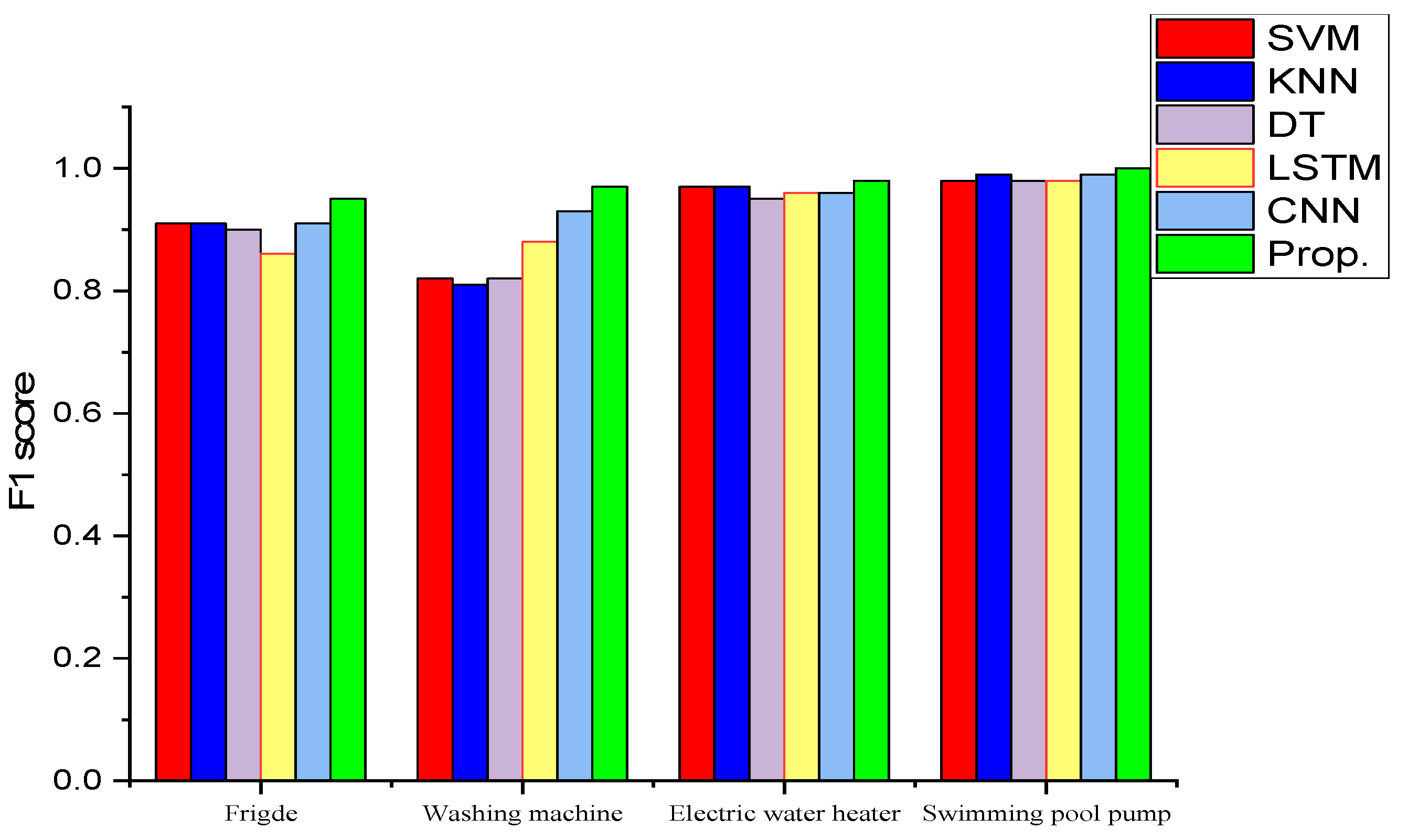
By analyzing the results presented in Table 7, Table 9, Table 10, Table 11, Table 13, and Table 15, we observed that all the models explored can detect the operating states of the different devices with good performance. To illustrate the effectiveness of the proposed method, the F1-score value achieved with the proposed method was compared with the other state-of-the-art classification methods. Figure 8 presents a comparative histogram of the different methods implemented.

For fridge, the best F1 score of 95% was achieved by the proposed technique, while LSTM achieved the worst F1 score of 86%. The other models classified the fridge with a similar F1 score of 91% for SVM, KNN, and CNN and 90% for DT.

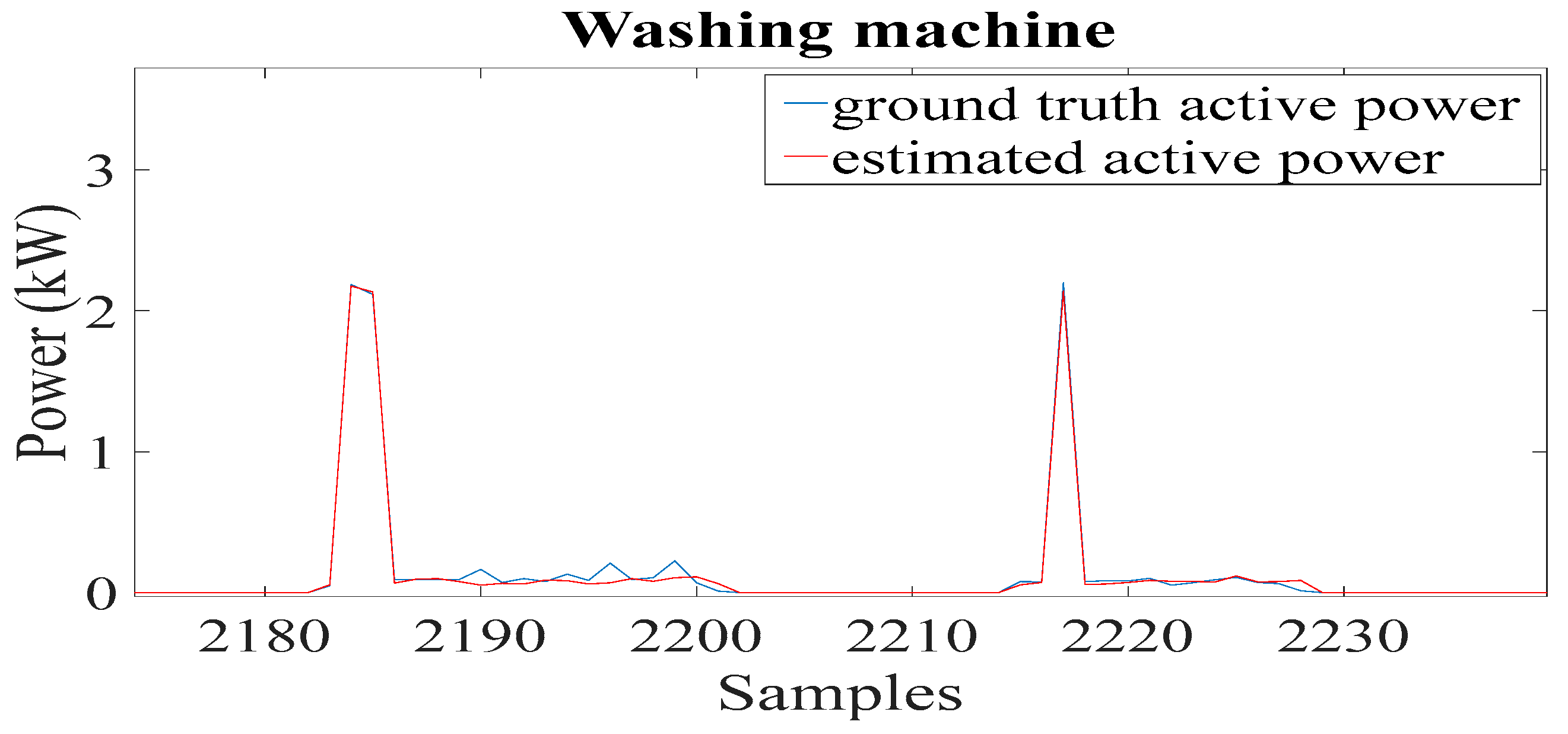
For washing machine, the proposed model obtained the best F1 score of 97%, while the SVM and decision tree models obtained similar F1 scores of 82%. Similarly, the two deep learning models obtained slightly better results than the SVM and decision tree models, with the CNN obtaining an F1 score of 93% and the LSTM an F1 score of 88%. The KNN model achieved the worst F1 score of 81%.

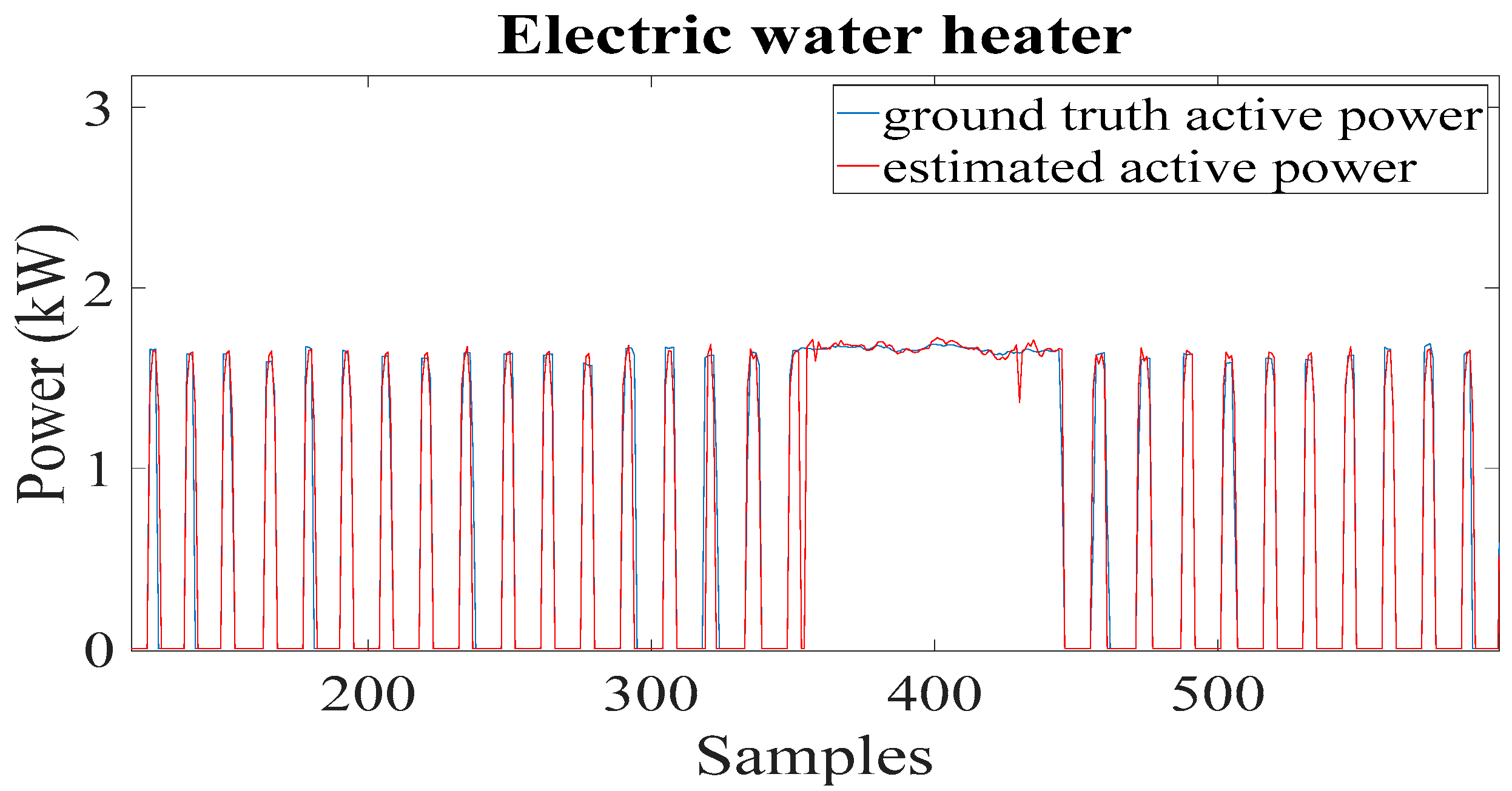
For the electric water heater, the proposed approach obtained an F1 score of 98% slightly higher than the F1 score of 97% obtained by the SVM and KNN models. The LSTM and CNN models had a comparable F1 score of 96%, and the decision tree model had the lowest F1 score of 95%.

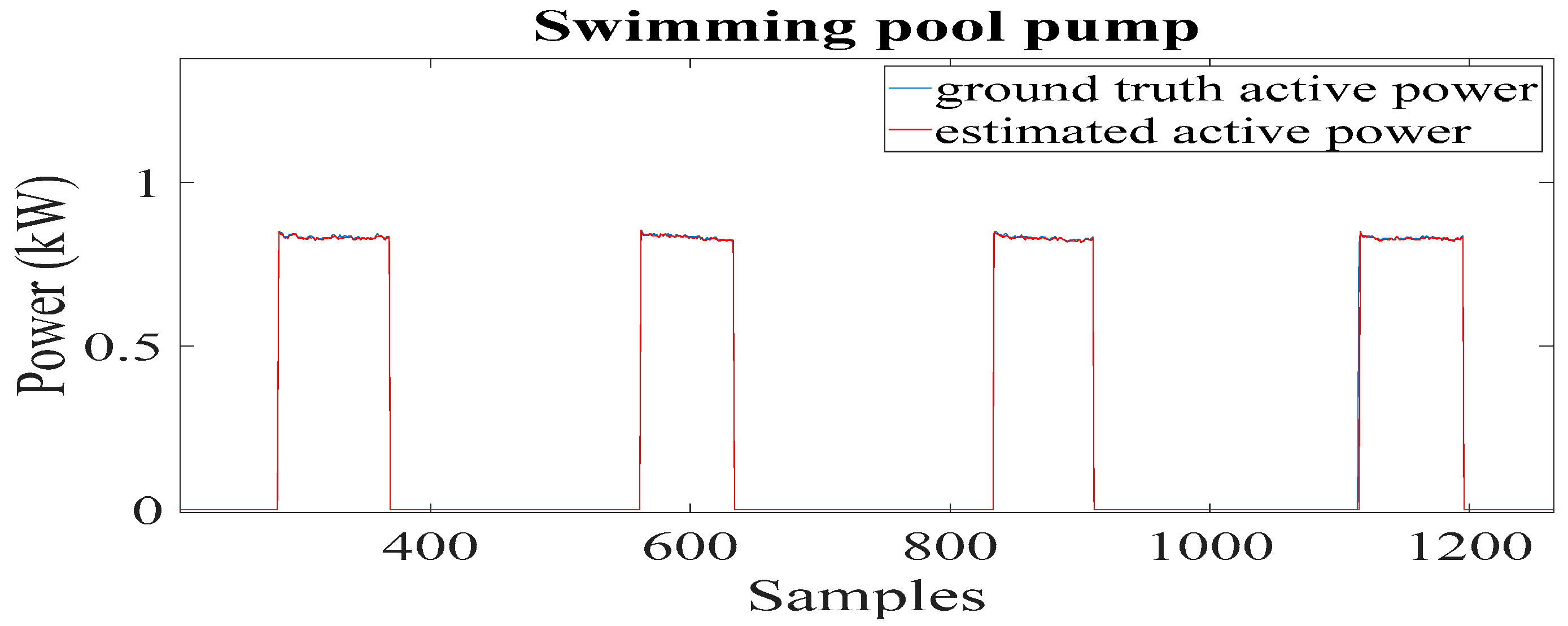
All the models performed well in the classification of the swimming pool pump, with an F1 score of more than 98% for the models SVM, KNN, decision tree, CNN, and LSTM and 100% for the proposed model. As can be seen, the best performances were obtained for high consumption devices, while most of the algorithms seemed to have more difficulties correctly detecting the washing machine and fridge activations. This is due to the complex architecture of these multi-state appliances, for which detection is a little more challenging for some models, resulting in a large number of false positives. Overall, it can be seen that the proposed framework achieved the best performance in terms of F1 score.

The performance of the six methods presented earlier was qualitatively comparable, as the same data were used for each one of the techniques. This is typically not the case when comparing the performance of state-of-the-art approaches found in the literature, as the data used and the context of these works are different. However, for the sake of illustration, a comparison with state-of-the-art approaches was conducted. It is also worth mentioning that the work reported in [43] used the same data as the case study described here but with different sampling periods (1 s in [43] and 1 min here). The washing machine and fridge are two popular multi-state devices for evaluating state-of-the-art NILM approaches, and they were used here.

Table 16. Washing machine performance comparison.

Approach	S (s)	Recall	Precision	F1	MAE (Wh)	SAE	EA
[27]	1	1	0.60	0.70	118.1	-	-
[41]	1	-	-	0.76	14.42	0.51	0.74
[42]	60	0.86	0.87	0.86	8.31	0.01	-
[43]	1	0.96	0.96	0.96	1.64	0.05	0.93
Proposed	60	0.97	0.97	0.97	1.1	0.03	0.93

S: sampling frequency.

compares the proposed NILM framework to some state-of-the-art NILM approaches for the washing machine. The fridge’s performance in comparison with state-of-the-art approaches is presented in

Table 17. Fridge performance comparison.

Approach	S (s)	Recall	Precision	F1	MAE (Wh)	SAE	EA
[27]	1	0.73	0.87	0.79	4.34	-	-
[41]	1	-	-	0.87	19.60	0.46	0.76
[42]	60	0.89	0.85	0.87	17.03	0.05	-
[43]	1	0.97	0.92	0.95	12.72	0.09	0.88
Proposed	60	0.98	0.91	0.95	4.00	0.01	0.96

. In both tables, the column labeled S(s) denotes the sampling time in seconds.

According to the analysis of the comparison results presented in Table 16 and Table 17, the proposed framework designed by MOGA performed better than the NILM method presented in [43] in terms of estimation accuracy for the fridge (96% versus 88% in [43]). The mean absolute error of the washing machine was reduced by 32% using the MOGA framework compared to the work presented in [43]. It should be noted that the proposed models designed by MOGA and the approach presented in [43] outperformed the other state-of-the-art methods referenced in Table 16 and Table 17.

Since the design of a radial basis function neural network by MOGA does not require too much training data (around 8212 samples to 24,493 samples) when using a sampling interval of one minute, while achieving a similar or better performance than approaches using more training data [43] (around 1.3 million samples to 1.4 million samples), it is worth noting that resampling the data sampling rate from 1 s to 1 min did not affect the performance of the MOGA framework and significantly reduced the amount of data to be processed.

It should be noted that MOGA is a time complex process. Although it runs on a computer cluster, the training of models with data sampled at 1 min takes several hours. As the complexity of MOGA is linear with the number of samples, the use of the same time period, sampled at one second, would translate the execution time to several days. In practice, MOGA cannot cope with this large number of samples, which would have the consequence of reducing the design data, diminishing in this way the number of events that could be used in the design process.

4.1. Test on AMPD Public Dataset

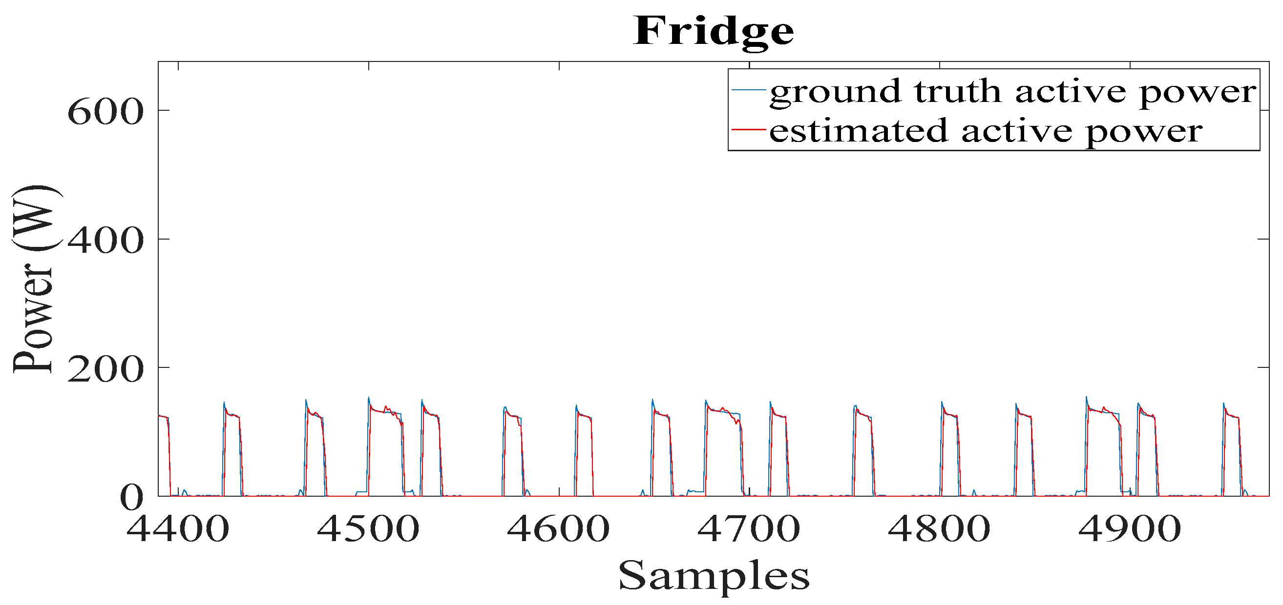
The proposed framework was also evaluated using the public dataset AMPD [82] (Almanac of Minutely Power datasets). It records a Canadian household’s water, natural gas, and electricity consumption data for two years, including electrical features such as voltage, current, active, and reactive power, collected at one-minute intervals. The data from 1 April 2012 to 30 April 2012 were considered. The models were trained using the same configuration as the proposed framework. Two appliances (fridge and clothes dryer) were considered in the experiment. The results of the test performed in the validation dataset in terms of energy estimation and device classification are presented in

Table 18. Results on AMPD public dataset.

Devices	MAE (Wh)	SAE	EA	Recall	Precision	F1
Fridge	9.13	0.10	0.90	0.91	0.93	0.92
Clothes dryer	3.53	0.01	0.94	0.99	1	0.99

.

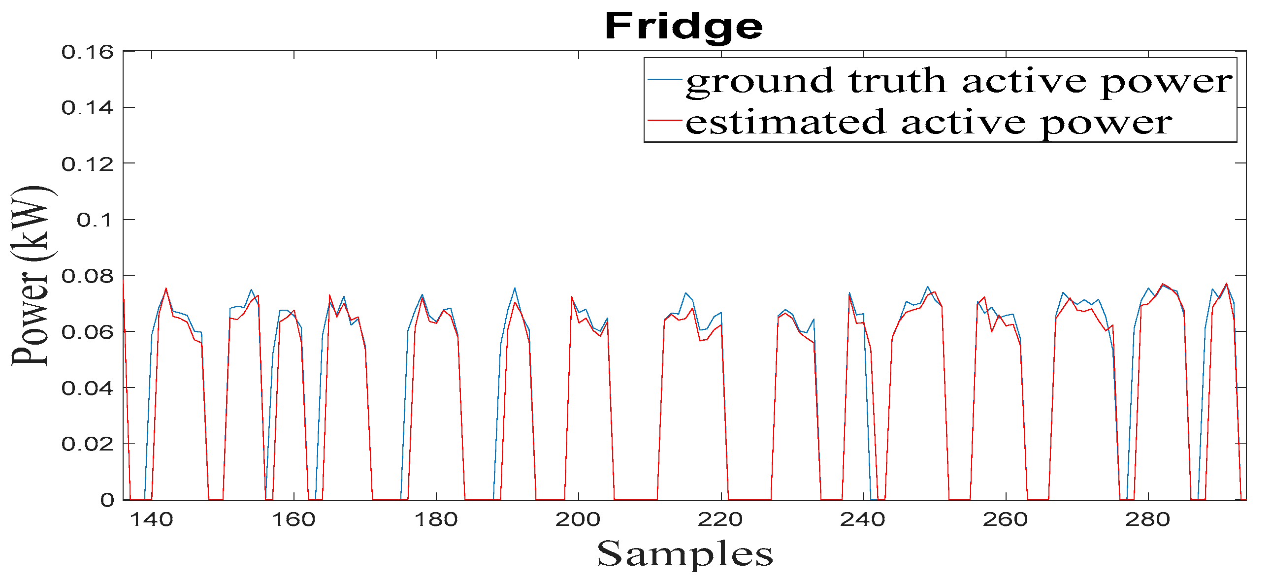
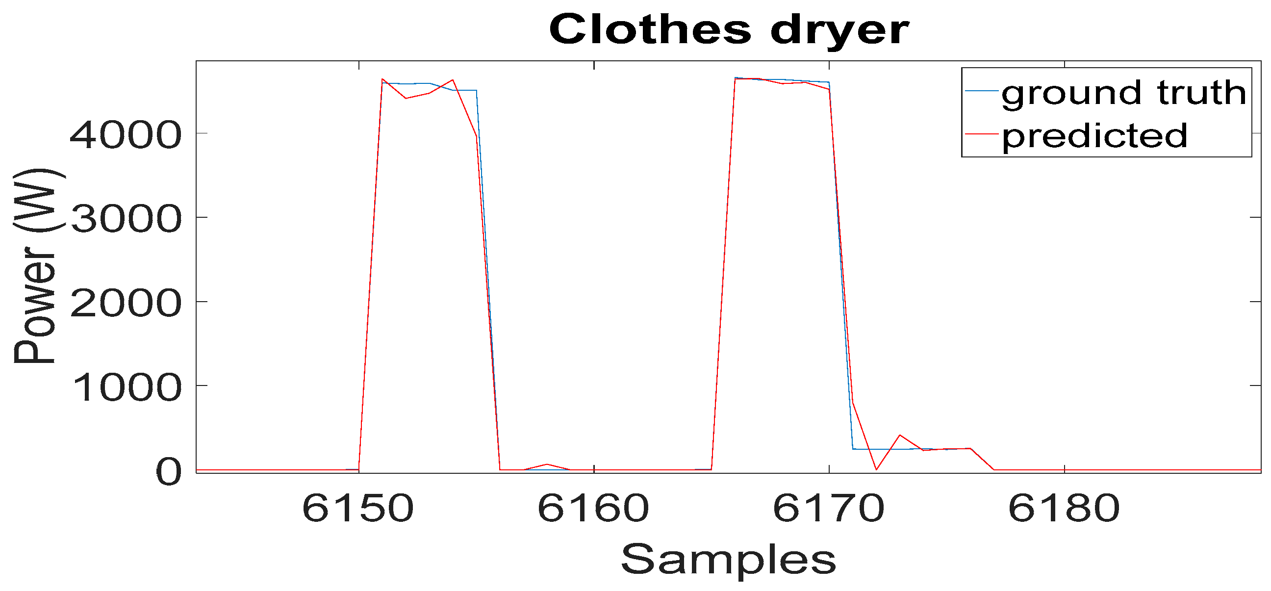
From the results in Table 18, it can be seen that the fridge and the clothes dryer were detected with a high F1 score of 0.92 and 0.99, respectively. Regarding the energy estimation, the fridge was estimated with an accuracy of more than 90%, while the clothes dryer was estimated with an accuracy of 94%.

Examples of disaggregation outputs, in terms of active power for the fridge, are presented in Figure 9. Figure 10 shows the example of disaggregation outputs for the clothes dryer.

There is a reasonably consistent agreement between the measured and estimated active power, as shown in Figure 9 and Figure 10.

The results obtained with this dataset were also compared to the work proposed in [53,83]. In both works, two weeks of data were used. In [83], the authors proposed a modified cross-entropy algorithm (MCE) based on a combinatorial optimization method to classify the load states. The approach consisted of searching for the best combination of states by iteratively updating the device’s operation probability to generate a load decomposition while considering the constraint of the penalty function. In [53], the authors suggested an approach based on the probability of time-segmented states. They used an affinity propagation clustering approach to extract the load power patterns, which were then used to count the probabilities of time-segmented states. After generating a range of appliance state matrices using probabilities, the function selects the most suitable matrix as the result of the appliance state detection.

Table 19. F1 comparison.

Devices	[53]	[83]	Proposed
Fridge	0.92	0.88	0.92
Clothes dryer	0.23	0.29	0.99

compares the results of the two appliances (fridge and clothes dryer) in terms of state identification (F1) with the references [53,83].

As illustrated in Table 19 for the fridge, the F1 score achieved by the proposed framework (92%) is comparable to the F1 score obtained by the Ref. [53], while the MCE [83] approach had the lowest score of 88%. For the clothes dryer, the proposed framework performed the best F1 score of 99%, while the Ref. [53] and MCE methods had the lowest scores of 23% and 29%, respectively. We concluded from these results that the proposed framework allowed us to achieve very satisfactory results.

4.2. Energy Consumption Estimation in the Case Study House

The procedure used to identify the four appliances discussed in Section 4 was extended to other devices in the case study house that consume the most electricity. One month of data was considered in the model design. The results generated by the data selection algorithm and the size of the datasets for each device for classification and estimation are presented in

Table 20. Data selection results for classification models.

Devices	CH Vertices	Training	Testing	Validation
AC_1	913	28,777	8925	8927
AC_2	1170	28,505	9501	9503
AC_3	569	26,777	8925	8927
AC_4	799	26,777	8925	8925
BS_1	714	26,777	8925	8927
BS_2	638	26,777	8925	8927
Oven	1164	26,777	8925	8927
DM	993	24,185	8061	8063
EAH_1	900	26,777	8925	8927
EAH_2	1386	26,777	8925	8927
EAH_3	1384	26,777	8925	8927

AC: Air conditioner, BS: Burner stove, DM: Drying machine, EAH: Electric air heater.

and

Table 21. Data selection results for estimation models.

Devices	CH Vertices	Training	Testing	Validation
AC_1	1993	26,777	8925	8927
AC_2	913	28,505	9501	9503
AC_3	543	26,777	8925	8927
AC_4	565	26,777	8925	8927
BS_1	881	26,777	8925	8927
BS_2	698	26,777	8925	8927
Oven	1249	26,777	8925	8927
DM	835	24,185	8061	8063
EAH_1	1982	26,777	8925	8927
EAH_2	1309	26,777	8925	8927
EAH_3	2180	26,777	8925	8927

, respectively.

After one run of MOGA, the non-dominated sets were generated. The size of the non-dominated sets for the classification models and energy estimation models are shown in

Table 22. Dimensions of non-dominated sets.

Devices	Classification	Estimation
AC_1	444	145
AC_2	281	86
AC_3	663	126
AC_4	131	159
BS_1	827	81
BS_2	256	256
Oven	539	213
DM	561	59
EAH_1	636	80
EAH_2	654	231
EAH_3	768	443

for each device.

Suitable models with good performance and low complexity were analyzed in the non-dominated sets. Two models (a classification and an estimation model) were selected for each device.

Table 23. Device state classification results.

Devices	Recall	Precision	F1	Nb of Features	Nb of Neurons	Model Complexity
AC_1	0.92	0.94	0.93	13	20	280
AC_2	0.97	0.98	0.97	5	30	180
AC _3	0.94	0.90	0.92	11	28	336
AC_4	1.00	1.00	1.00	9	11	110
BS_1	0.59	0.81	0.68	5	23	138
BS_2	0.86	0.97	0.91	12	29	377
Oven	0.80	0.97	0.88	19	29	580
DM	0.96	0.98	0.97	17	29	522
EAH_1	0.98	0.95	0.96	4	30	150
EAH_2	0.91	0.89	0.90	9	30	300
EAH_3	0.74	0.76	0.75	9	18	180

shows the results of the device state classification using the selected models in terms of model complexity, number of neurons in the hidden layer, number of features, recall, precision, and F1 score. The results in terms of device energy estimation using the selected models are shown in

Table 24. Energy estimation results.

Devices	MAE (Wh)	SAE	EA	Nb of Features	Nb of Neurons	Model Complexity
AC_1	191.0	0.011	0.87	14	18	270
AC_2	11.0	0.002	0.97	3	17	68
AC _3	11.0	4 × 10−4	0.98	7	10	80
AC_4	9.0	0.003	0.97	15	18	288
BS_1	90.0	0.004	0.86	3	20	80
BS_2	37.0	0.002	0.90	3	4	16
Oven	43.0	0.005	0.73	22	19	437
DM	0.009	4 × 10−4	0.98	3	9	36
EAH_1	28.0	0.010	0.95	12	13	169
EAH_2	10.0	0.004	0.99	3	12	48
EAH_3	14.0	0.006	0.87	16	6	102

.

Analyzing the classification results presented in Table 23, we observed an excellent F1 score of 100% for the air conditioner (AC-4), whereas the lowest F1 scores were observed in the classification of the burner stove (BS-1: 68%) and the electric air heater (EAH-3: 75%). In the first case, a higher sampling frequency should be used, while in the second case, the device is rarely activated and there is a lack of identifiable data. The other appliances were classified with good F1 scores ranging from 88% to 98%. The results reported in Table 24 show that the electric air heater (EAH-2) was estimated with an excellent estimation accuracy (EA) of 99%. The lowest performance was observed in the disaggregation of the oven (73%). This is due to the fact that the oven has several different operating modes, with different consumptions together with a large range of temperatures. The other devices were estimated with good estimation accuracy ranging from 86% to 98%.

Once the models were designed, the energy consumption of certain appliances in the case study house was estimated using these models. The aggregated data from January 2022 were considered in the experiment.

Table 25. Distribution of energy consumption in the case study house.

Phase	Appliances	E (kWh)
	Air conditioner (AC1)	11.97
	Air conditioner (AC2)	91.98
I	Burner stove (BS1)	14.42
	Electric air heater (EAH1)	24.56
	Electric air heater (EAH3)	28.40
	Electric air heater (EAH2)	95.52
	Drying machine (DM)	13.36
	Electric water heater (EWH)	114.54
II	Fridge	17.80
	Washing machine (WM)	13.73
	Swimming pool pump (SPP)	153.14
	Oven	19.22
	Air conditioner (AC3)	16.32
III	Air conditioner (AC4)	71.74
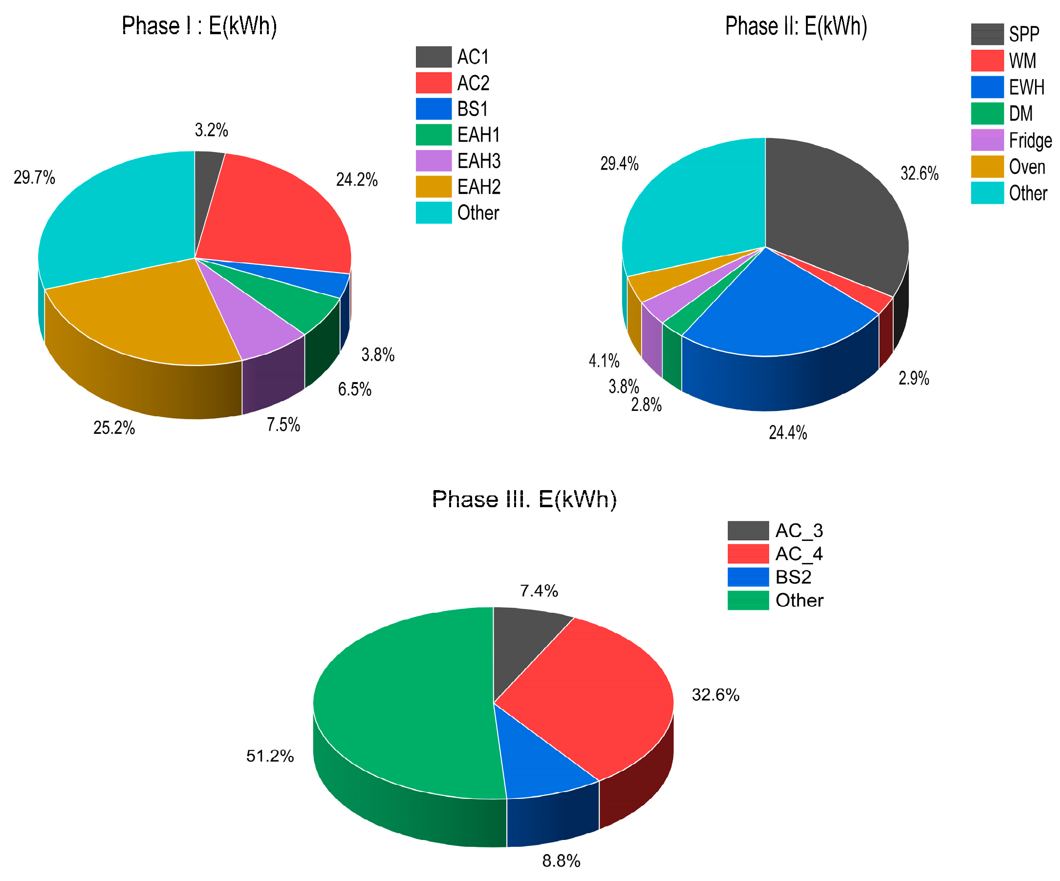
	Burner stove (BS2)	19.27

shows the results of the disaggregation in terms of appliance energy consumption. Since the aggregated data were measured by the EM340 three-phase smart meter, the distribution of appliance consumption by phase is presented.

Analyzing the disaggregation results reported in Table 25, it can be seen that the highest energy consumption in the month of January 2022 was assigned to the swimming pool pump (153.14 kWh) followed by the electric water heater (114.54 kWh). The electric air heater (EHA2) and air conditioners (AC2 and AC4) consumed approximately 11.97 kWh, 91.98 kWh, and 71.74 kWh respectively. The consumption of the other appliances was estimated between 4.22 kWh and 28.40 kWh. Figure 11 presents pie charts summarizing the distribution of electricity consumption in the case study house in the month of January 2022.

The total consumption of the house, during the month of January 2022, was 1070 kWh, divided into 380, 470, and 220 kWh for Phases 1 to 3. The appliances considered in this section account for 66% of the total monthly consumption. Besides being responsible for most of the electric energy consumption in the household, most of these appliances are schedulable, meaning that their operation can be changed without causing much trouble for the occupants. This is the case with HVAC appliances (AC 1-4, EAH 1-3, WM, DM, SPP, and, to a less extent, EWH). These appliances account for 60% of the house’s total consumption, which means that there is considerable flexibility in shaping the house electric profile to meet energy management goals. As the house in question has PV panels and electric storage, the online operation of some of these electric appliances is taken into account in our proposed model-based predictive control of HEMS [84].

5. Conclusions

In this study, a low complexity NILM framework based on radial basis function neural networks designed by a multi-objective genetic algorithm (MOGA) was proposed for energy disaggregation. Despite reducing the data sampling from one second to one minute to allow for the use of low-cost meters, the reduction of design time, and the employment of low complexity models, the proposed technique presented an excellent ability to disaggregate the usage of devices.

A comparative analysis of other computational intelligence classifiers for non-intrusive load monitoring, using the same data, showed that the proposed framework obtained the best experimental results in terms of appliance identification. The comparison with other state-of-the-art methods, both using different data and common data, highlighted the efficiency of the proposed framework in achieving the best estimation of the energy consumed by each device in the house.

The proposed NILM technique was used to disaggregate one month of consumption of the house, and it was able to identify the operation of appliances accounting for 2/3 of the electric consumption. It allowed us also to recognize that around 60% of the consumption was related to schedulable appliances, therefore allowing an additional flexibility for the HEMS available in the residence.

Future work will be devoted to the question of the transferability of the proposed framework to other houses, as well as its integration in the house HEMS. One additional advantage of using very simple models is that their real time execution is in the order of a few milliseconds in standard computer architectures, which allows an edge implementation.

References

1. Liu, H. Introduction. In Non-Intrusive Load Monitoring: Theory, Technologies and Applications; Liu, H., Ed.; Springer: Singapore, 2020; pp. 1–21. [Google Scholar] [CrossRef]
2. Meng, F.; Chen, S.; Cheng, S.; Chen, B.; Li, Z.; Wang, F.; Liu, G. Analysis of subnational CO2 mitigation policy pressure in the residential sector in China. J. Clean. Prod. 2021, 293, 126203. [Google Scholar] [CrossRef]
3. Deng, Q.; Alvarado, R.; Toledo, E.; Caraguay, L. Greenhouse gas emissions, non-renewable energy consumption, and output in South America: The role of the productive structure. Environ. Sci. Pollut. Res. 2020, 27, 14477–14491. [Google Scholar] [CrossRef]
4. Zhai, Q.; Li, T.; Liu, Y. Life cycle assessment of a wave energy converter: Uncertainties and sensitivities. J. Clean. Prod. 2021, 298, 126719. [Google Scholar] [CrossRef]
5. Balezentis, T. Shrinking ageing population and other drivers of energy consumption and CO2 emission in the residential sector: A case from Eastern Europe. Energy Policy 2020, 140, 111433. [Google Scholar] [CrossRef]
6. Santiago, I.; Lopez-Rodriguez, M.A.; Trillo-Montero, D.; Torriti, J.; Moreno-Munoz, A. Activities related with electricity consumption in the Spanish residential sector: Variations between days of the week, Autonomous Communities and size of towns. Energy Build. 2014, 79, 84–97. [Google Scholar] [CrossRef]
7. Zhao, X.; Gao, W.; Qian, F.; Ge, J. Electricity cost comparison of dynamic pricing model based on load forecasting in home energy management system. Energy 2021, 229, 120538. [Google Scholar] [CrossRef]
8. Gomes, I.; Bot, K.; Ruano, M.d.G.; Ruano, A. Recent Techniques Used in Home Energy Management Systems: A Review. Energies 2022, 15, 2866. [Google Scholar] [CrossRef]
9. Franco, P.; Martínez, J.M.; Kim, Y.-C.; Ahmed, M.A. IoT based approach for load monitoring and activity recognition in smart homes. IEEE Access 2021, 9, 45325–45339. [Google Scholar] [CrossRef]
10. Laouali, I.H.; Qassemi, H.; Marzouq, M.; Ruano, A.; Bennani, S.D.; El Fadili, H. A survey on computational intelligence techniques for non intrusive load monitoring. In Proceedings of the 2020 IEEE 2nd International Conference on Electronics, Control, Optimization and Computer Science, ICECOCS 2020, Kenitra, Morocco, 2–3 December 2020. [Google Scholar]
11. Zhou, X.; Li, S.; Liu, C.; Zhu, H.; Dong, N.; Xiao, T. Non-Intrusive Load Monitoring Using a CNN-LSTM-RF Model Considering Label Correlation and Class-Imbalance. IEEE Access 2021, 9, 84306–84315. [Google Scholar] [CrossRef]
12. Esa, N.F.; Abdullah, M.P.; Hassan, M.Y. A review disaggregation method in Non-intrusive Appliance Load Monitoring. Renew. Sustain. Energy Rev. 2016, 66, 163–173. [Google Scholar] [CrossRef]
13. Zoha, A.; Gluhak, A.; Imran, M.A.; Rajasegarar, S. Non-intrusive Load Monitoring approaches for disaggregated energy sensing: A survey. Sensors 2012, 12, 16838–16866. [Google Scholar] [CrossRef] [PubMed] [Green Version]
14. Zeifman, M.; Roth, K. Nonintrusive appliance load monitoring: Review and outlook. IEEE Trans. Consum. Electron. 2011, 57, 76–84. [Google Scholar] [CrossRef]
15. Ruano, A.; Hernandez, A.; Ureña, J.; Ruano, M.; Garcia, J. NILM Techniques for Intelligent Home Energy Management and Ambient Assisted Living: A Review. Energies 2019, 12, 2203. [Google Scholar] [CrossRef] [Green Version]
16. Hart, G.W. Prototype Nonintrusive Appliance Load Monitor: Progress Report 2; MIT Energy Laboratory: Concord, MA, USA, 1985. [Google Scholar]
17. Hart, G.W. Nonintrusive Appliance Load Monitoring. Proc. IEEE 1992, 80, 1870–1891. [Google Scholar] [CrossRef]
18. Athanasiadis, C.; Doukas, D.; Papadopoulos, T.; Chrysopoulos, A. A scalable real-time non-intrusive load monitoring system for the estimation of household appliance power consumption. Energies 2021, 14, 767. [Google Scholar] [CrossRef]
19. Athanasiadis, C.L.; Papadopoulos, T.A.; Doukas, D.I. Real-time non-intrusive load monitoring: A light-weight and scalable approach. Energy Build. 2021, 253, 111523. [Google Scholar] [CrossRef]
20. Völker, B.; Pfeifer, M.; Scholl, P.M.; Becker, B. FIRED: A Fully-Labeled HIgh-FRequency Electricity Disaggregation Dataset. In Proceedings of the 7th ACM International Conference on Systems for Energy-Efficient Buildings, Cities, and Transportation, Virtual Event Japan, 18–20 November 2020; Association for Computing Machinery: New York, NY, USA; pp. 294–297. [Google Scholar]
21. Kim, H.; Marwah, M.; Arlitt, M.; Lyon, G.; Han, J. Unsupervised Disaggregation of Low Frequency Power Measurements. In Proceedings of the 2011 SIAM International Conference on Data Mining, Philadelphia, PA, USA, 28–30 April 2011; pp. 747–758. [Google Scholar]
22. Kolter, J.Z.; Jaakkola, T. Approximate inference in additive factorial HMMs with application to energy disaggregation. In Proceedings of the 15th International Conference on Artificial Intelligence and Statistics (AISTATS) 2012, La Palma, Spain, 21–23 April 2012. [Google Scholar]
23. Zoha, A.; Gluhak, A.; Nati, M.; Imran, M.A. Low-power appliance monitoring using Factorial Hidden Markov Models. In Proceedings of the 2013 IEEE 8th International Conference on Intelligent Sensors, Sensor Networks and Information Processing: Sensing the Future, ISSNIP 2013, Melbourne, Australia, 2–5 April 2013. [Google Scholar]
24. Parson, O.; Ghosh, S.; Weal, M.; Rogers, A. Non-Intrusive Load Monitoring Using Prior Models of General Appliance Types. In Proceedings of the Twenty-Sixth AAAI Conference on Artificial Intelligence, Toronto, ON, Canada, 22–26 July 2012; pp. 356–362. [Google Scholar]
25. Makonin, S.; Popowich, F.; Bajic, I.V.; Gill, B.; Bartram, L. Exploiting HMM Sparsity to Perform Online Real-Time Nonintrusive Load Monitoring. IEEE Trans. Smart Grid 2016, 7, 2575–2585. [Google Scholar] [CrossRef]
26. Bonfigli, R.; Principi, E.; Fagiani, M.; Severini, M.; Squartini, S.; Piazza, F. Non-intrusive load monitoring by using active and reactive power in additive Factorial Hidden Markov Models. Appl. Energy 2017, 208, 1590–1607. [Google Scholar] [CrossRef]
27. Mengistu, M.A.; Girmay, A.A.; Camarda, C.; Acquaviva, A.; Patti, E. A Cloud-based On-line Disaggregation Algorithm for Home Appliance Loads. IEEE Trans. Smart Grid 2018, 10, 3430–3439. [Google Scholar] [CrossRef]
28. Figueiredo, M.B.; De Almeida, A.; Ribeiro, B. An experimental study on electrical signature identification of non-intrusive load monitoring (NILM) systems. Lect. Notes Comput. Sci. Incl. Subser. Lect. Notes Artif. Intell. Lect. Notes Bioinform. 2011, 6594 LNCS, 31–40. [Google Scholar] [CrossRef]
29. Moradzadeh, A.; Zeinal-Kheiri, S.; Mohammadi-Ivatloo, B.; Abapour, M.; Anvari-Moghaddam, A. Support vector machine-assisted improvement residential load disaggregation. In Proceedings of the 2020 28th Iranian Conference on Electrical Engineering (ICEE), Tabriz, Iran, 4–6 August 2020; pp. 1–6. [Google Scholar] [CrossRef]
30. Lin, Y.H.; Tsai, M.S. Applications of hierarchical support vector machines for identifying load operation in nonintrusive load monitoring systems. In Proceedings of the 2011 9th World Congress on Intelligent Control and Automation, Taipei, Taiwan, 21–25 June 2011; pp. 688–693. [Google Scholar] [CrossRef]
31. Srinivasan, D.; Ng, W.S.; Liew, A.C. Neural-network-based signature recognition for harmonic source identification. IEEE Trans. Power Deliv. 2005, 21, 398–405. [Google Scholar] [CrossRef]
32. Lemes, D.A.M.; Cabral, T.W.; Fraidenraich, G.; Meloni, L.G.P.; De Lima, E.R.; Neto, F.B. Load Disaggregation Based on Time Window for HEMS Application. IEEE Access 2021, 9, 70746–70757. [Google Scholar] [CrossRef]
33. Giri, S.; Bergés, M.; Rowe, A. Towards automated appliance recognition using an EMF sensor in NILM platforms. Adv. Eng. Inform. 2013, 27, 477–485. [Google Scholar] [CrossRef]
34. Le, T.-T.-H.; Kim, H. Non-Intrusive Load Monitoring Based on Novel Transient Signal in Household Appliances with Low Sampling Rate. Energies 2018, 11, 3409. [Google Scholar] [CrossRef] [Green Version]
35. Liu, H. Machine Learning Based Appliance Identification. In Non-Intrusive Load Monitoring: Theory, Technologies and Applications; Liu, H., Ed.; Springer: Singapore, 2020; pp. 141–162. [Google Scholar] [CrossRef]
36. Azad, S.A.; Ali, A.B.M.S.; Wolfs, P. Identification of typical load profiles using K-means clustering algorithm. In Proceedings of the Asia-Pacific World Congress on Computer Science and Engineering, APWC on CSE 2014, Nadi, Fiji, 4–5 November 2014. [Google Scholar] [CrossRef]
37. He, K.; Stankovic, L.; Liao, J.; Stankovic, V. Non-Intrusive Load Disaggregation Using Graph Signal Processing. IEEE Trans. Smart Grid 2018, 9, 1739–1747. [Google Scholar] [CrossRef]
38. Zhang, B.; Zhao, S.; Shi, Q.; Zhang, R. Low-rate non-intrusive appliance load monitoring based on graph signal processing. In Proceedings of the 2019 International Conference on Security, Pattern Analysis, and Cybernetics, SPAC 2019, Guangzhou, China, 20–23 December 2019; pp. 11–16. [Google Scholar] [CrossRef]
39. Mauch, L.; Yang, B. A new approach for supervised power disaggregation by using a deep recurrent LSTM network. In Proceedings of the 2015 IEEE Global Conference on Signal and Information Processing (GlobalSIP), Orlando, FL, USA, 14–16 December 2015; pp. 63–67. [Google Scholar]
40. Kelly, J.; Knottenbelt, W. Neural NILM: Deep Neural Networks Applied to Energy Disaggregation. arXiv 2015, arXiv:1507.06594. [Google Scholar]
41. Rafiq, H.; Shi, X.; Zhang, H.; Li, H.; Ochani, M.K. A deep recurrent neural network for non-intrusive load monitoring based on multi-feature input space and post-processing. Energies 2020, 13, 2195. [Google Scholar] [CrossRef]
42. Massidda, L.; Marrocu, M.; Manca, S. Non-intrusive load disaggregation by convolutional neural network and multilabel classification. Appl. Sci. 2020, 10, 1454. [Google Scholar] [CrossRef] [Green Version]
43. Laouali, I.; Ruano, A.; Ruano, M.d.G.; Bennani, S.D.; Fadili, H.E. Non-Intrusive Load Monitoring of Household Devices Using a Hybrid Deep Learning Model through Convex Hull-Based Data Selection. Energies 2022, 15, 1215. [Google Scholar] [CrossRef]
44. Gomes, E.; Pereira, L. PB-NILM: Pinball guided deep non-intrusive load monitoring. IEEE Access 2020, 8, 48386–48398. [Google Scholar] [CrossRef]
45. Pereira, L.; Nunes, N. Performance evaluation in non-intrusive load monitoring: Datasets, metrics, and tools—A review. Wiley Interdiscip. Rev. Data Min. Knowl. Discov. 2018, 8, e1265. [Google Scholar] [CrossRef] [Green Version]
46. Klemenjak, C.; Reinhardt, A.; Pereira, L.; Makonin, S.; Bergés, M.; Elmenreich, W. Electricity consumption data sets: Pitfalls and opportunities. In Proceedings of the 6th ACM International Conference on Systems for Energy-Efficient Buildings, Cities, and Transportation, New York, NY, USA, 3–14 November 2019; pp. 159–162. [Google Scholar]
47. De la Prieta, F.; Vale, Z.; Antunes, L.; Pinto, T.; Campbell, A.T.; Julián, V.; Neves, A.J.R.; Moreno, M.N. Trends in Cyber-Physical Multi-Agent Systems. The PAAMS Collection–15th International Conference, PAAMS 2017.; Springer International Publishing: Cham, Switzerland, 2018; Volume 619, pp. 3–6. [Google Scholar] [CrossRef]
48. Le, T.-T.-H.; Kang, H.; Kim, H. Household Appliance Classification Using Lower Odd-Numbered Harmonics and the Bagging Decision Tree. IEEE Access 2020, 8, 55937–55952. [Google Scholar] [CrossRef]
49. Hassan, T.; Javed, F.; Arshad, N. An Empirical Investigation of V-I Trajectory Based Load Signatures for Non-Intrusive Load Monitoring. IEEE Trans. Smart Grid 2014, 5, 870–878. [Google Scholar] [CrossRef] [Green Version]
50. Himeur, Y.; Alsalemi, A.; Bensaali, F.; Amira, A. Robust event-based non-intrusive appliance recognition using multi-scale wavelet packet tree and ensemble bagging tree. Appl. Energy 2020, 267, 114877. [Google Scholar] [CrossRef]
51. Chang, H.; Lian, K.; Su, Y.; Lee, W. Power-Spectrum-Based Wavelet Transform for Nonintrusive Demand Monitoring and Load Identification. IEEE Trans. Ind. Appl. 2014, 50, 2081–2089. [Google Scholar] [CrossRef]
52. Kong, W.; Dong, Z.Y.; Hill, D.J.; Luo, F.; Xu, Y. Improving nonintrusive load monitoring efficiency via a hybrid programing method. IEEE Trans. Ind. Inform. 2016, 12, 2148–2157. [Google Scholar] [CrossRef]
53. Liu, L.; Li, F.; Cheng, Z.; Zhou, Y.; Shen, J.; Li, R.; Xiong, S. Non-Intrusive Load Monitoring Method Considering the Time-Segmented State Probability. IEEE Access 2022, 10, 39627–39637. [Google Scholar] [CrossRef]
54. Lindahl, P.A.; Green, D.H.; Bredariol, G.; Aboulian, A.; Donnal, J.S.; Leeb, S.B. Shipboard Fault Detection Through Nonintrusive Load Monitoring: A Case Study. IEEE Sens. J. 2018, 189, 8986–8995. [Google Scholar] [CrossRef]
55. Khosravani, H.R.; Ruano, A.E.; Ferreira, P.M. A convex hull-based data selection method for data driven models. Appl. Soft Comput. J. 2016, 47, 515–533. [Google Scholar] [CrossRef]
56. Kelly, J.; Batra, N.; Parson, O.; Dutta, H.; Knottenbelt, W.; Rogers, A.; Singh, A.; Srivastava, M. NILMTK v0.2: A non-intrusive load monitoring toolkit for large scale data sets: Demo abstract. In Proceedings of the 1st ACM Conference on Embedded Systems for Energy-Efficient Buildings, Memphis, Tennessee, 3–6 November 2014; pp. 182–183. [Google Scholar]
57. Mestre, G.; Ruano, A.; Duarte, H.; Silva, S.; Khosravani, H.; Pesteh, S.; Ferreira, P.M.; Horta, R. An intelligent weather station. Sensors 2015, 15, 31005–31022. [Google Scholar] [CrossRef] [Green Version]
58. Eft-Systems: Battery BoxHV. Available online: https://www.eft-systems.de/en/B-BOX%20Premium/product/Battery%20Box%20HVS-HVM/6 (accessed on 1 November 2022).
59. Ruano, A.; Silva, S.; Duarte, H.; Ferreira, P.M. Wireless Sensors and IoT Platform for Intelligent HVAC Control. Appl. Sci. 2018, 8, 370. [Google Scholar] [CrossRef] [Green Version]
60. Company, C.G.A. EM340 Utilises Touchscreen Technology. Available online: https://www.carlogavazzi.co.uk/blog/carlo-gavazzi-energy-solutions/em340-utilises-touchscreen-technology (accessed on 4 July 2022).
61. Circutor Wibee: Consumption Analyzers. Available online: https://circutor.com/en/articles/wibeee-your-consumptions-in-the-palm-of-your-hand/ (accessed on 1 November 2022).
62. Ruano, A.; Bot, K.; Ruano, M.G. Home Energy Management System in an Algarve Residence. First Results. In Proceedings of the CONTROLO 2020, Bragança, Portugal, 1–3 July 2020; Springer: Cham, Switzerland, 2020; pp. 332–341. [Google Scholar]
63. Ferreira, P.M.; Ruano, A.E. Exploiting the separability of linear and nonlinear parameters in radial basis function networks. In Proceedings of the IEEE 2000 Adaptive Systems for Signal Processing, Communications, and Control Symposium, AS-SPCC 2000, Lake Louise, AB, Canada, 4 October 2000; pp. 321–326. [Google Scholar] [CrossRef]
64. Teixeira, C.A.; Ruano, M.G.; Ruano, A.E.; Pereira, W.C.A. A soft-computing methodology for noninvasive time-spatial temperature estimation. IEEE Trans. Biomed. Eng. 2008, 55, 572–580. [Google Scholar] [CrossRef] [PubMed]
65. Levenberg, K.; Arsenal, F. A method for the solution of certain non-linear problems in least squares. Quart. Appl. Math 1944, 2, 164–168. [Google Scholar] [CrossRef]
66. Harkat, H.; Ruano, A.E.; Ruano, M.G.; Bennani, S.D. GPR target detection using a neural network classifier designed by a multi-objective genetic algorithm. Appl. Soft Comput. J. 2019, 79, 310–325. [Google Scholar] [CrossRef]
67. Bot, K.; Ruano, A.; Da, M.; Ruano, G. Short-Term Forecasting Photovoltaic Solar Power for Home Energy Management Systems. Inventions 2021, 6, 12. [Google Scholar] [CrossRef]
68. Ferreira, P.M.; Ruano, A.E. Evolutionary Multiobjective Neural Network Models Identification: Evolving Task-Optimised Models. Stud. Comput. Intell. 2011, 372, 21–53. [Google Scholar] [CrossRef]
69. Cortes, C.; Vapnik, V. Support-vector networks. Mach. Learn. 1995, 20, 273–297. [Google Scholar] [CrossRef]
70. Huang, X.; Maier, A.; Hornegger, J.; Suykens, J.A.K. Indefinite kernels in least squares support vector machines and principal component analysis. Appl. Comput. Harmon. Anal. 2017, 43, 162–172. [Google Scholar] [CrossRef] [Green Version]
71. Guo, G.; Wang, H.; Bell, D.; Bi, Y.; Greer, K. KNN Model-Based Approach in Classification. In Proceedings of the on the Move to Meaningful Internet Systems 2003: CoopIS, DOA, and ODBASE, Sicily, Italy, 3–7 November 2003; pp. 986–996. [Google Scholar]
72. Yang, C.C.; Soh, C.S.; Yap, V.V. A systematic approach in appliance disaggregation using k-nearest neighbours and naive Bayes classifiers for energy efficiency. Energy Effic. 2018, 11, 239–259. [Google Scholar] [CrossRef]
73. Quinlan, J.R. Induction of decision trees. Mach. Learn. 1986, 1, 81–106. [Google Scholar] [CrossRef] [Green Version]
74. Hochreiter, S. Long Short-Term Memory. Neural Comput. 1997, 1780, 1735–1780. [Google Scholar] [CrossRef] [PubMed]
75. Graves, A.; Schmidhuber, J. Framewise phoneme classification with bidirectional LSTM and other neural network architectures. Neural Netw. 2005, 18, 602–610. [Google Scholar] [CrossRef] [PubMed]
76. Stratigakos, A.; Bachoumis, A.; Vita, V.; Zafiropoulos, E. Analysis and LSTM Neural Networks. Energies 2021, 14, 4107. [Google Scholar] [CrossRef]
77. Krizhevsky, A.; Sutskever, I.; Hinton, G.E. ImageNet Classification with Deep Convolutional Neural Networks. Proc. Adv. Neural Inf. Process. Syst. 2012, 25, 1097–1105. [Google Scholar] [CrossRef] [Green Version]
78. Simonyan, K.; Zisserman, A. Very deep convolutional networks for large-scale image recognition. In Proceedings of the 3rd International Conference on Learning Representations, ICLR 2015–Conference Track Proceedings, San Diego, CA, USA, 7–9 May 2015; pp. 1–14. [Google Scholar]
79. Liu, H. Deep Learning Based Appliance Identification. In Non-Intrusive Load Monitoring; Springer: Singapore, 2020; pp. 191–214. [Google Scholar]
80. Kong, W.; Dong, Z.Y.; Wang, B.; Zhao, J.; Huang, J. A practical solution for non-intrusive type II load monitoring based on deep learning and post-processing. IEEE Trans. Smart Grid 2020, 11, 148–160. [Google Scholar] [CrossRef]
81. Makonin, S.; Popowich, F. Nonintrusive load monitoring performance evaluation A unified approach for accuracy reporting. Energy Effic. 2015, 8, 809–814. [Google Scholar] [CrossRef]
82. Makonin, S.; Ellert, B.; Bajić, I.V.; Popowich, F. Electricity, water, and natural gas consumption of a residential house in Canada from 2012 to 2014. Sci. Data 2016, 3, 160037. [Google Scholar] [CrossRef] [Green Version]
83. Machlev, R.; Levron, Y.; Beck, Y. Modified cross-entropy method for classification of events in NILM systems. IEEE Trans. Smart Grid 2018, 10, 4962–4973. [Google Scholar] [CrossRef]
84. Bot, K.; Laouali, I.; Ruano, A.; Ruano, M.d.G. Home Energy Management Systems with Branch-and-Bound Model-Based Predictive Control Techniques. Energies 2021, 14, 5852. [Google Scholar] [CrossRef]
Figure 1. NILM overview.
Energies 15 09073 g001
Figure 2. Overview of the proposed approach.
Energies 15 09073 g002
Figure 3. Overview of the design approach.
Energies 15 09073 g003
Figure 4. Fridge: blue, ground truth active power; red, estimated active power.
Energies 15 09073 g004
Figure 5. Washing machine: blue, ground truth active power; red, estimated active power.
Energies 15 09073 g005
Figure 6. Electric water heater: blue, ground truth active power; red, estimated active power.
Energies 15 09073 g006
Figure 7. Swimming pool pump: blue, ground truth active power; red, estimated active power.
Energies 15 09073 g007
Figure 8. F1 comparison.
Energies 15 09073 g008
Figure 9. Fridge AMPD: blue, ground truth active power; red, estimated active power.
Energies 15 09073 g009
Figure 10. Clothes dryer AMPD: blue, ground truth active power; red, estimated active power.
Energies 15 09073 g010
Figure 11. Distribution of electricity consumption.
Energies 15 09073 g011