Article

Influence of Shading on Solar Cell Parameters and Modelling Accuracy Improvement of PV Modules with Reverse Biased Solar Cells

School of Engineering, Cardiff University, Cardiff CF24 3AA, UK
*
Author to whom correspondence should be addressed.
Energies 2022, 15(23), 9067; https://doi.org/10.3390/en15239067
Submission received: 27 October 2022 / Revised: 23 November 2022 / Accepted: 24 November 2022 / Published: 30 November 2022
(This article belongs to the Section A2: Solar Energy and Photovoltaic Systems)

Abstract

:
This paper presents an experimental investigation on the influence of shading on mono-crystalline (mono-Si) solar cell parameters. The variations of equivalent circuit parameters with shading were determined and then used in modelling a mono-Si solar cell and a mono-Si photovoltaic (PV) module under partial shading. It was found that the simulation by considering the parameter variations with shading in the single cell model did not lead to a noticeable improvement in modelling accuracy. However, for the PV module, a significant improvement in modelling accuracy in the reverse bias region was achieved when considering all parameter variations in the model. A further investigation was performed to identify the key parameters that are responsible for the improvement. The results revealed that in addition to the photo-generated current, the shunt resistance also has a significant effect on the model accuracy. A modelling approach was thus proposed, which includes the variation of the shunt resistance with shading, in addition to the variation of the photo-generated current. This approach was experimentally validated using a mono-Si PV module. The results show that the proposed approach is more accurate, compared to the approach that considers only the variation of the photo-generated current, without the need to include an avalanche breakdown term.

1. Introduction

Photovoltaic (PV) technology converts solar energy into electricity. It is one of the major contributors to the electricity generation worldwide. The main advantage of PV technology is that it can be used everywhere around the globe due to the unlimited availability of sunlight. In addition, PV technology can be used with a variety of power ratings thanks to its modularity feature [1]. The partial shading of PV panels is an inevitable issue that is caused by blocking the light from reaching the solar cells by neighboring objects, such as trees and buildings, etc. [2]. Partial shading has a negative impact on the output power of PV systems, in addition to other issues, such as hot spots, which could lead to a damage of the shaded solar cells due to high temperatures [3]. Furthermore, it makes the maximum power point tracking (MPPT) an intricate task due to the fact that the output characteristics of the partially shaded PV systems exhibit multiple maximum power points (MPPs) [4]. Therefore, modelling the electrical response of the PV systems under partial shading provides useful information in understanding their behavior under real operation, calculating energy yield [4] and evaluating the effectiveness of MPPT techniques [5].
A literature survey revealed that there are numerous partial shading models proposed. They widely differ in terms of the modelling procedure and size of the PV systems [4]. The equivalent circuit model that consists of a single diode with five parameters is commonly used for the modelling of solar cells [6,7,8,9,10,11,12,13,14,15,16,17,18,19,20,21,22,23,24,25,26,27] and herein referred to as the single diode five-parameter model. The model can be further simplified to reduce the computational burdens by omitting the shunt resistance [28]. Moreover, the double diode equivalent circuit model [5,29,30,31,32,33,34,35] employs an additional diode to consider the recombination that occurs in the space charge region of the solar cells [2]. This model improves the modelling accuracy, particularly under low irradiance, at the expense of increasing the number of parameters that need to be determined and the consequently modelling complexity [5].
Figure 1 depicts the equivalent circuit of the single diode five-parameter model. The circuit consists of a current source representing the current generated by light, a diode representing the p-n junction, and two resistances—the series resistance ( R s ) and shunt resistances ( R sh ), representing the losses of the solar cells [2,36].
The output current ( I ) of a solar cell can be expressed as [1,2]:
I = I ph I D   I sh   =   I ph     ( exp (   V + IR s nV th ) 1 )     ( V + IR s R sh )
where, I ph is the photo-generated current, I D is the current flowing through the diode, I sh   is the current flowing through the shunt resistance,   I s is the reverse saturation current, V is the output voltage, n is the ideality factor and V th is the thermal voltage, which is given by [1,2,36]:
V th = kT q
where, T is the cell temperature in Kelvin scale, k is the Boltzmann constant, and q is the electron charge. The five parameters in Equation (1) are R s , R sh , n ,   I s , and I ph , which determine the current-voltage (I-V) characteristics of the equivalent circuit.
In partial shading modelling, most of the published models use a single solar cell as the basic unit to model the PV systems [6,7,8,9,10,12,14,15,16,18,19,20,21,22,24,25,26,29,31,32,33,34]. In addition, most of these models do not account for the variation of the equivalent circuit parameters with shading. They assumed that the photo-generated current of the solar cell is the only parameter that changes with shading. The other four parameters (i.e., R s , R sh , n , and I s ) are assumed constant. Two exceptions in this aspect are the works reported in [20,27]. In the work by Wang et al. [20], the effect of frame shadow cast on a photovoltaic-thermal system was investigated. In addition to I ph , the variation of R s and R sh with shading was also included. However, there was no assessment on which parameter, R s or R sh , had more influence on the model accuracy. In the work by Bharadwaj et al. [27], they proposed a model of a PV module under partial shading at a sub-cell level. Each solar cell is divided into several sub-cells connected in parallel and the variation of R s , R sh ,   I s , and I ph was taken into account using the estimated values from the calculation. In addition, no assessment was made to identify the parameters, whose variation has significant impact on model accuracy.
An alternative approach is to include the avalanche breakdown effect originally proposed by Bishop [6] to model the shading influence. This avalanche breakdown is added as a multiplication term connected in series with the shunt resistance of the equivalent circuit shown in Figure 1. This approach has proved to be sufficiently accurate to model the shaded solar cells if this term is added to the single diode five-parameter model [6,25] or to the double diode model [31]. A similar concept that adds the avalanche breakdown term in parallel with the shunt resistance was reported in [29] and implemented in the works using a single diode five-parameter model [7,19,22] and a double diode model [32]. The drawback of this approach is that the breakdown voltage needs to be determined. Since this voltage varies significantly among the solar cells, even if they are from the same batch [37] or within the same module [38], it is not available in the datasheet of the PV manufacturers. Moreover, the determination of this voltage needs the dark reverse bias measurements of the solar cells [38] and thus it is not readily available.
Clearly, it is more practical to explore the possibility of improving the model accuracy of shading, based on the single diode five-parameter model that does not require the avalanche breakdown term. In addition, it is beneficial to identify which equivalent circuit parameter plays a dominant role in affecting the model accuracy of the shading behavior. This paper presents an experimental study to determine the variation of the equivalent circuit parameters with shading, followed by a detailed examination of the model improvement by taking into account the shading effect on the equivalent circuit parameters. The effect of the parameter variation with shading for each parameter was investigated separately, in order to identify these that have a major impact on the model accuracy of the shading behavior.

2. Experimental

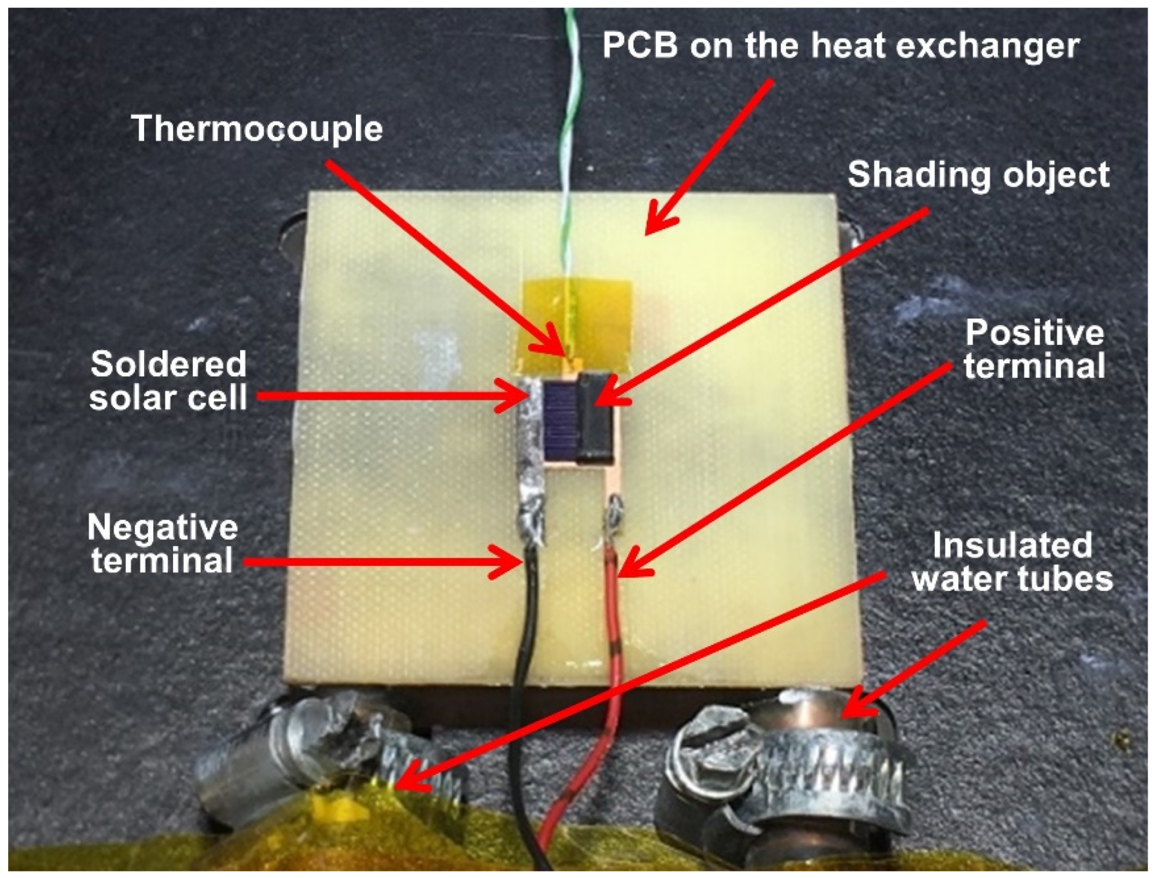
2.1. Solar Cells Preparation

The mono-Si solar cells used in this work were supplied as a cut-wafer with a single front busbar. Since solar cells are very brittle, it is necessary to support them mechanically to avoid cell breakage. A printed circuit board (PCB) was used to hold the cell and facilitate contact soldering following the work of [39] who used a direct copper bonded (DCB) board. The PCB was designed using SolidWorks software and fabricated by the Electrical Workshop at Cardiff University. The back contact of the cell was soldered to the PCB using a hot-plate by heating the PCB and the cell with the solder in between. The front wire ribbon and terminal wires were soldered to the copper pad on the PCB using a soldering iron. A K-type thermocouple was attached to the copper pad and then the cell assembly was mounted on a water-cooled copper heat exchanger with thermal paste (2.9 W/(m·K)) in between. Figure 2 shows a completed cell testing assembly, which was placed under the light source for the partial shading experiment. The shading block shown in Figure 2 was fabricated using 3D printing.

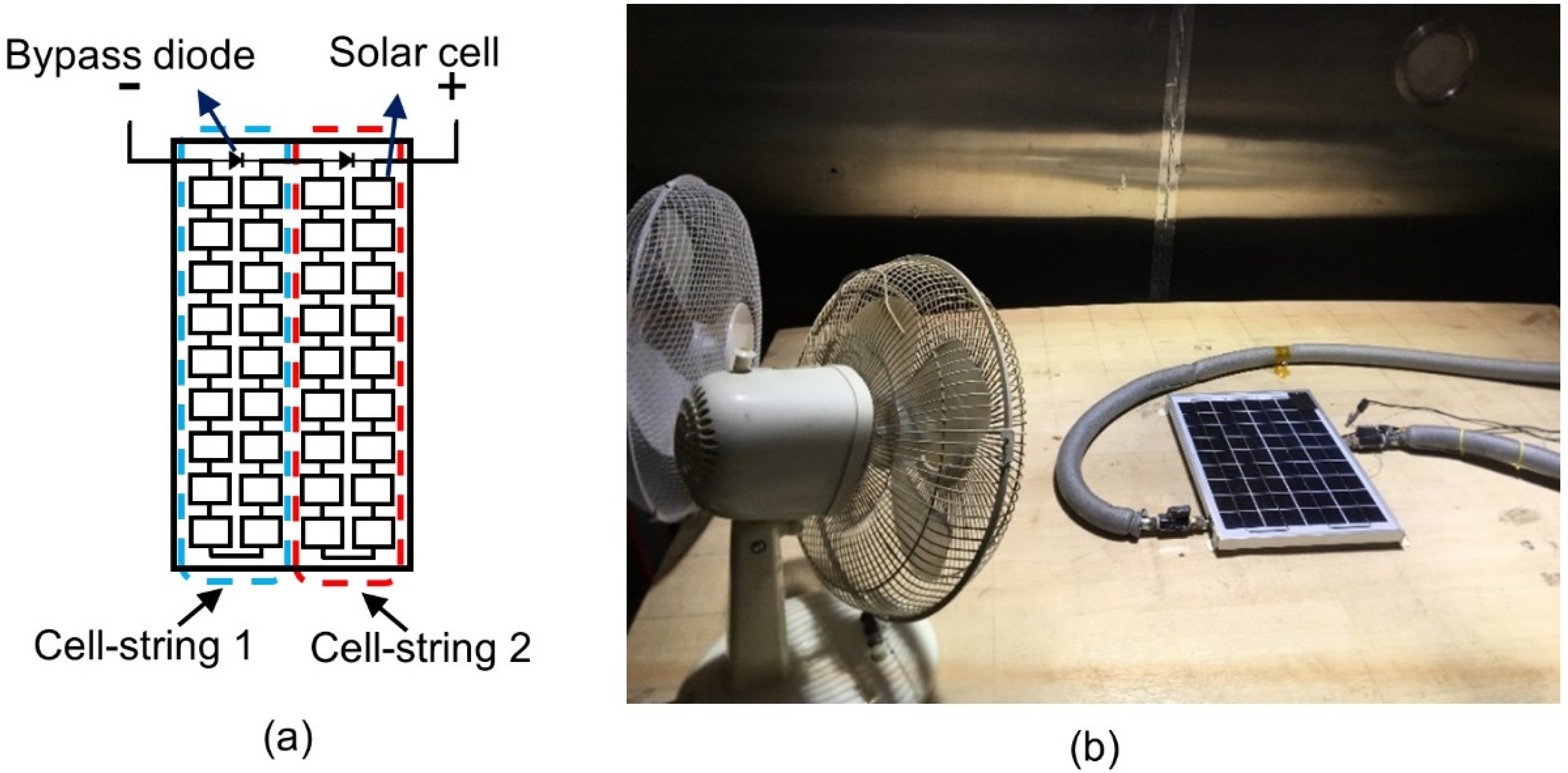
2.2. PV Module Preparation

The PV module used in this work for the partial shading investigation was a 10 W commercial module from Betop-camp that has a total dimension of 34 cm × 24 cm and 36 mono-Si solar cells connected in series. The module was divided into two cell-strings of 18 cells each and a bypass diode (IN5819) was soldered to each cell-string. A K-type thermocouple was attached to the back of the module for monitoring the testing temperature. A water-cooled aluminium heat exchanger was attached to the back of the module with the thermal paste between the gaps. The water was supplied to the heat exchanger using insulated tubes. To perform the partial shading experiments, the PV module testing assembly was placed under the light source. The module is placed at the centre of a calibrated area (see Appendix A) The partial shading was accomplished by applying an adhesive black foam tape onto the part of the solar cell surface where it is to be shaded. Figure 3a shows the configuration of the cells and bypass diodes, and Figure 3b shows a photograph of the module under the shading experiment. The two fans were added to improve the cooling effectiveness so that the module temperature can be maintained at 25 °C for a sufficient amount of time to complete the measurements.

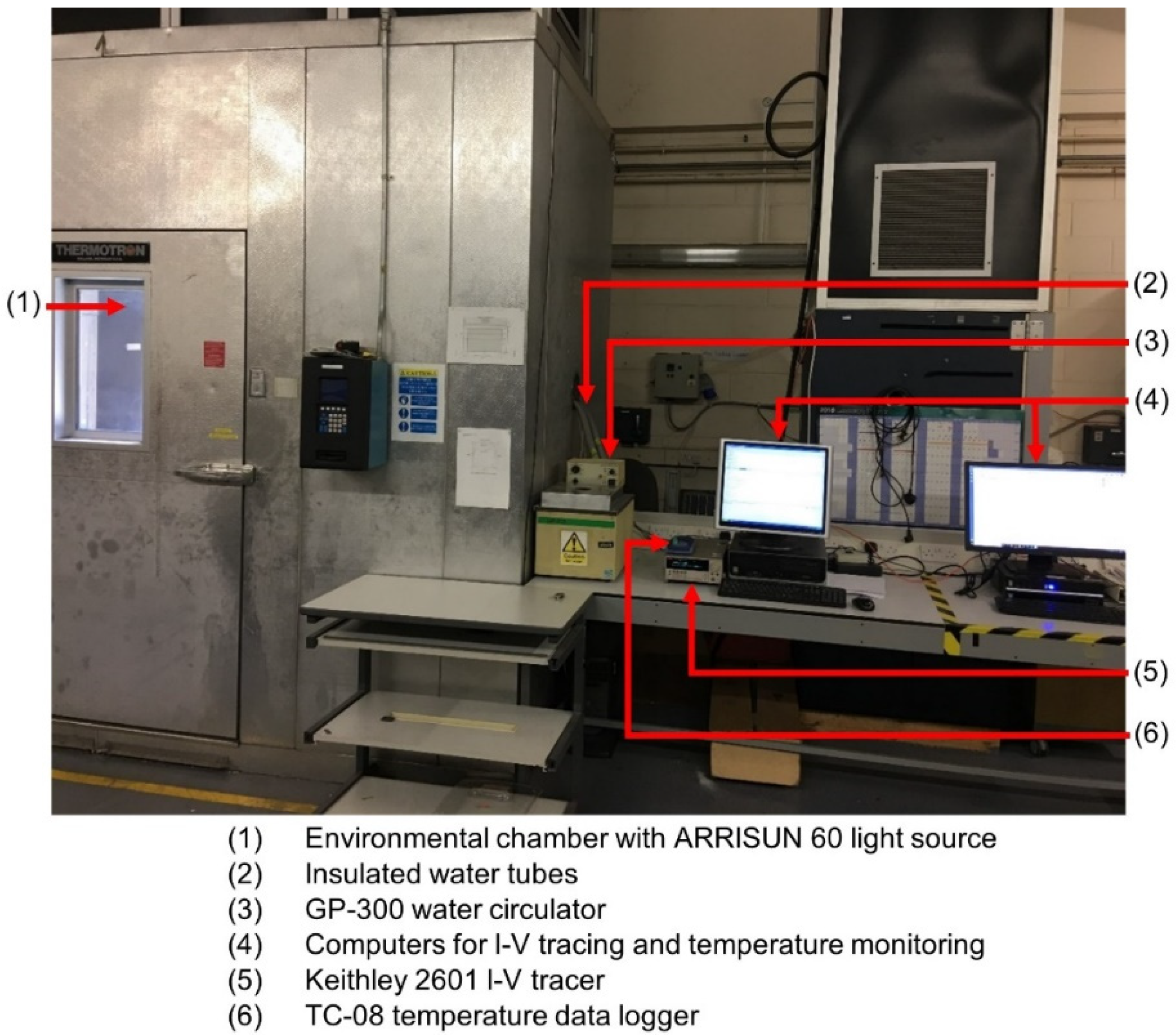
2.3. Experimental Set-Up

The experimental set-up for characterising the solar cells and modules is depicted in Figure 4. The light source (ARRISUN 60, ARRI, Munich, Germany) used in this work is a rare-earth hot-restrike lamp (6000 HR UNP), which is located at the top of an environmental chamber. The light source was calibrated, in terms of the spectral match, spatial non-uniformity and temporal instability, based on the E927-10 standards. It was found to be of Class BCA for the area that is suitable for the characterisation of all solar cells used in this research. For the 10 W PV module characterisation, the spatial non-uniformity was estimated as 18.9% (see Appendix A for details). Although this value is above the Class C limit (10%) of the E927-10 standards, the non-uniformity at this level did not cause any noticeable distortion to the shape of the I-V curves of the PV module when measured without shading. In addition, the characteristic shape (such as the slope) of the I-V curves of the PV module remains nearly the same when the partial shading was applied to different solar cells, which are under a slightly different irradiance, due to non-uniformity. This behavior indicates that the non-uniformity at this level has no impact on the data reliability of this study (see Appendix B for details).
For the solar cell testing, the light source irradiance was first measured at the centre of a table inside the chamber using a reference cell (Solar Survey 200R, Seaward Electronic Limited, Co. Durham, UK) and set to 1000 W/m2 by adjusting an electronic ballast that regulates the lamp power. Then, the cell testing assembly described in Section 2.1 was placed in the centre of the table under the calibrated light intensity. The insulated water tubes were connected to a water circulator (GP-300) located outside the chamber. The insulation of the tubes is necessary to avoid the heating of the water by the light. The cell temperature was monitored using a thermocouple connected to a data logger (TC-08) and a computer. The I-V curves were measured using a Keithley source meter (2601) controlled by the computer using a special software. The PV module testing employs the same procedures as that of the solar cell testing described above, with the light irradiance of 1000 W/m2 measured at the centre of the module using the reference cell.

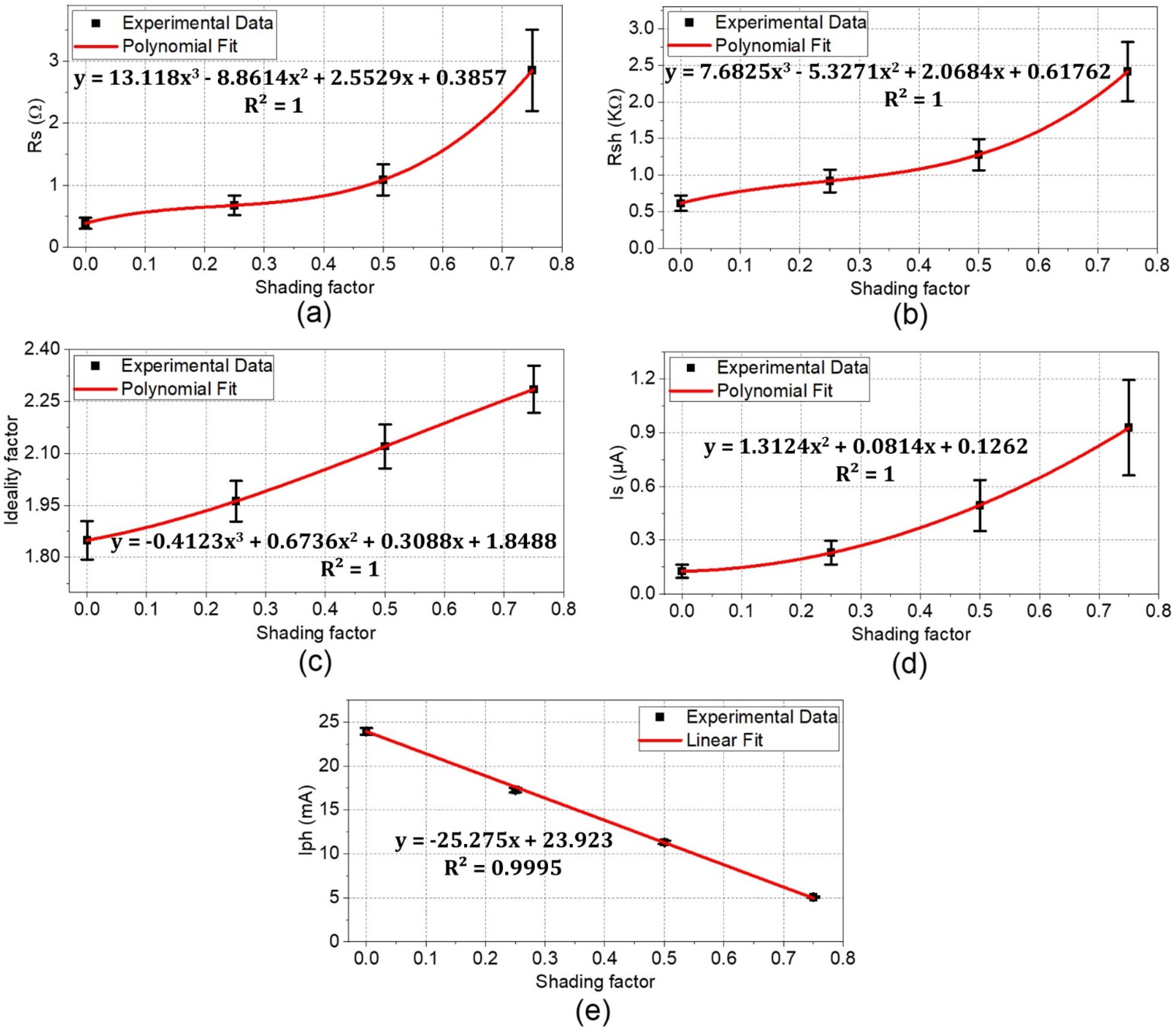
3. Effect of Shading on the Solar Cell Parameters

The solar cell used in this study has an active area of 0.78 cm2 (0.78 cm × 1 cm) as shown in Figure 2. The shading effect on five parameters in the single diode model (i.e., R s , R sh , n ,   I s , and I ph ) were investigated. The parameters were extracted from experimental I-V curves using the analytical method reported in [40], which is an improved version of [41]. In addition, the maximum power ( P max ), short circuit current ( I sc ), open circuit voltage ( V oc ), fill factor ( FF ), efficiency, and characteristic resistance ( R ch ), were also extracted from the experimental I-V curves.
The I-V curve was first measured without shading at standard test conditions (STCs), which is defined as the irradiance of 1000 W/m2, air mass (AM) of 1.5, and solar cell temperature of 25 °C [42]. The purpose of this experiment is to determine the errors of the facility for the I-V measurements. Twelve measurements were carried out with four measurements obtained per day in three days, during which the facility was shut down after testing each day. The relative standard deviation (RSD) for each parameter was calculated from the 12 measurements.
The partial shading experiment was performed by measuring the I-V curves with the active area of the solar cell blocked by 0%, 25%, 50% and 75%, respectively. The shading block was made using 3D printing (Ultimaker 2 Extended Plus, Ultimaker, Utrecht, Holland), which has a resolution of 12.5   μ m . The shading block was positioned on the solar cell with the assistance of a high-quality ruler and magnifying glass, which has an error of 0.2–0.3 mm. In addition, the correct percentage of the shading can be “verified” by checking the corresponding percentage of the short circuit current with respect to the non-shading case because the short circuit current changes linearly with the light intensity. Three I-V curves were measured for each shading case. The parameters were extracted from the average I-V curve of the three measurements. All I-V measurements were conducted in STCs and the whole procedure was repeated on another day to ensure the reliability of the test. The average value for each parameter was calculated and presented as a function of the shading factor, α = A sh   / A T   , where A sh   is the shaded area of the cell and A T   is the total cell area [26].
Figure 5a,e depict the equivalent circuit parameters as a function of the shading factor. The error bars in the figures were determined from 12 measurements, as described earlier. Since the error bars do not overlap in most cases, it is clear that the changes in the parameters are due to the shading effect. The fitting equation of each parameter, together with the corresponding coefficient of determination ( R 2 ), are also shown in the figures. It can be seen in Figure 5a,b that both R s and R sh increase with the increasing shading area. The variation of R s is broadly in agreement with the data reported in [26], but the rate of the increase is higher in the present work. This may be attributed to different solar cells used for the investigations. A similar variation in R s was also observed in [43], where a mono-Si cell was investigated under a reduced irradiance. It is to be noted that the partial shading and reducing the irradiance have the same effect on the parameters if the total light power is the same for both cases [44]. However, the variation of R sh exhibits a different behavior in [43]. Moreover, the variation of R sh reported in [45,46] shows a good agreement with our results, although it was derived from the PV module testing under varying irradiance. It can be seen in Figure 5c that the ideality factor, n , increases approximately linearly with shading. It remains within the typical value (between 1 and 2) of crystalline silicon solar cells [2] for shading up to 25%. However, it exceeds this bound for shading of >30%. Figure 5d,e show that the reverse saturation current,   I s , increases with shading, whereas the photo-generated current, I ph , decreases linearly with shading, as expected.
Figure 6a,f show the variation of the performance parameters with shading alongside the fitting equations and R 2 . It can be seen that P max   and I sc   decrease linearly with shading. As a result, the efficiency also decreases linearly with shading. However, V oc   and FF exhibit a nonlinear decrease with shading. The decrease of V oc   is consistent with the findings of another work [20]. R ch   increases with shading in a similar way to these observed in R s and R sh .

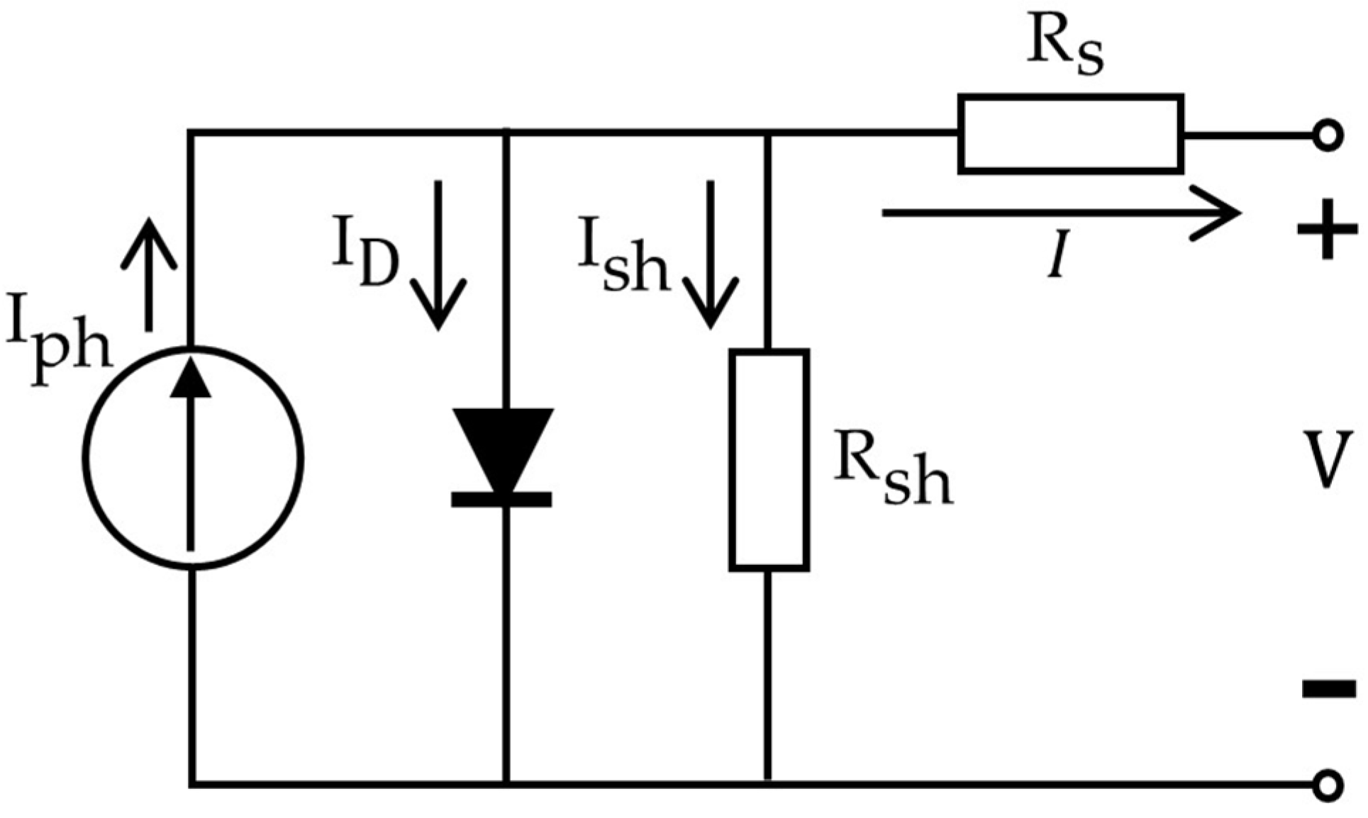
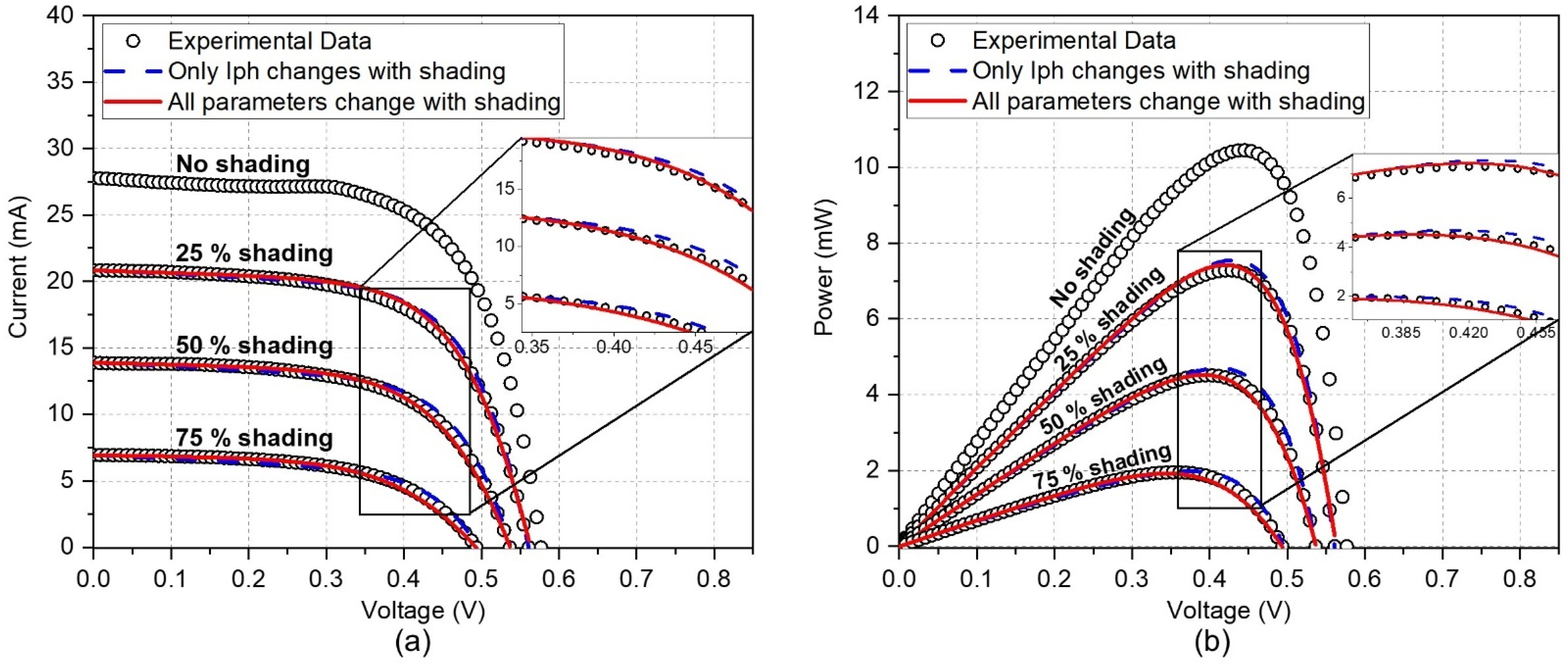
4. Single Cell Model by Considering the Parameter Variation with Shading

When a solar cell is partially shaded, the overall irradiance on the cell is reduced. As previously mentioned, it has been shown that the effect of partial shading on the solar cell performance is the same as an equivalent irradiance reduction without shading [44]. Thus, when modelling a solar cell under partial shading, we can add the shading factor ( α ) to the solar cell equation (Equation (1)) to represent the irradiance reduction, due to shading in a similar way to [26]. However, the work of [26] considered the effect of shading on the photo-generated current only. In this work, we considered the effect of shading on all five parameters in the solar cell equation. Using the experimental data presented in Figure 5a,e, the empirical relations between the equivalent circuit parameters and the shading factor were obtained as follows:
R s   = ( 34.0109   R so   α 3 ) ( 22.9749   R so   α 2 ) + ( 6.6189   R so   α ) + R so
R sh   = ( 12.4389   R sho   α 3 ) ( 8.6252   R sho   α 2 ) + ( 3.349   R sho   α ) + R sho
n = ( 0.223   n o   α 3 ) + ( 0.3643   n o   α 2 ) + ( 0.167   n o   α ) + n o
I s   =   ( 10.3994   I so   α 2 ) + ( 0.645   I so   α ) + I so
I ph   =   I pho   ( 1     α )
where   R so   ,   R sho   ,   n o   , I so   , and I pho   are the equivalent circuit parameters determined under the no shading condition. To evaluate the improvement of the model by taking into account the variation of all five parameters with shading, a mono-Si solar cell from a different batch to the one used to obtain the results of Figure 5a,e was selected to perform a comparative study between the model simulation and experiment. The cell has an active area of 0.8 cm2 (0.8 cm × 1 cm) and the testing assembly was prepared using the same procedure described in Section 2.1. Table 1 lists the five parameters of the cell determined from the experimental I-V curve in STCs without shading.
The theoretical I-V curves under 25%, 50%, and 75% shading were calculated using Equation (1) with the five parameters defined by Equations (3)–(7) and the non-shading values from Table 1. Equation (1) was solved in MATLAB using a publicly available program [47], based on the Newton Raphson method. The calculated I-V and power-voltage (P-V) curves are compared with the corresponding experimental results in Figure 7a,b. For comparison, the I-V and P-V curves were also calculated by using the fixed equivalent circuit parameters listed in Table 1, except for changing I ph   with shading. It can be seen that both calculated curves show a good agreement with the experimental results. The model that takes into account the variation of all parameters with shading does not provide a better fit than the model that takes into account the variation of I ph   only. This indicates that considering the effect of shading on I ph   alone can provide sufficient accuracy for modelling the shading effect at the solar cell level. However, it is interesting to note that this is not the case at module level, as discussed in Section 5.2.

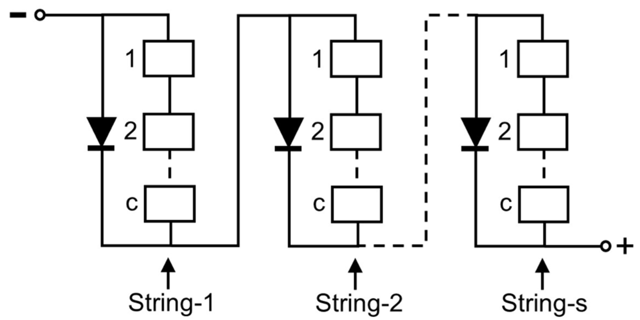
5. PV Module Model by Considering the Parameter Variation with Shading

A PV module consists of multiple solar cells that are usually connected in series. It is anticipated that the partial shading of a solar cell will affect the cell differently from a PV module because the change caused by the partial shading in a cell will interact with the rest of the unshaded cells. Clearly, it is important to investigate the effect of the partial shading on a PV module where the variation of all equivalent circuit parameters is taken into consideration. The parameter variation with shading described by Equations (3)–(6) was used for this study.

5.1. PV Module Modelling Procedure

The model for the PV module used in this study was developed using MATLAB, based on a well-established approach [19,20,21,25,26,27], which calculates the voltage of each cell according to its shading state and then adds the voltage of all cells to obtain the total module voltage. The calculation procedure can be illustrated using a PV module configuration shown in Figure 8 [21], which consists of s number of cell-strings and each cell-string consists of c number of solar cells connected in series and protected by a bypass diode. The calculation steps are described as follows.
Once the five parameters of the PV module under the non-shading condition are determined from its experimental I-V curve, the corresponding parameters for single cells are derived from dividing the obtained values of R s and R sh by the number of total cells in the module [48]. Subsequently, the parameters of the shaded cell or cells are adapted to the actual shading condition, using Equations (3)–(7). The voltage of each cell ( V cell ) is then calculated, based on its photo-generated current ( I ph , cell ), which depends on the shading percentage, from a piecewise approach presented in [21,26] and can be described using the single diode five-parameter model by:
  V cell   = {   Solve   for   V cell   :   [ 0 = I ph , cell   I s ( exp (   IR s + V cell   nV th ) 1 ) (   IR s + V cell   R sh )   I   ]   if   0     I     I ph , cell       [ ( R sh ( I I ph , cell   ) )   ]   IR s   if   I   >   I ph , cell  
Equation (8) implies that the cell is in a normal operation if 0     I     I ph , cell   , whereas it is in the reverse bias operation, due to shading, if I   >   I ph , cell   .
The next step is to determine the photo-generated current of each cell-string ( I ph , st ), which is equal to the minimum I ph , cell   among all cells in the cell-string, thus [27]:
I ph , st   = min   ( I ph , cell )  
The voltage of each cell-string ( V st ) is then calculated, according to its I ph , st   from a piecewise method presented in [21]:
V st   = { i = 1 c   V cell , i     if   0     I     I ph , st     i = 1   c   V cell , i     if   (   I   >   I ph , st   )   and   ( i = 1 c   V cell , i       V D   ) V D     if   (   I   >   I ph , st   )   and   ( i = 1 c   V cell , i   <   V D   )  
where,   V D   is the voltage of the bypass diodes, which is 0.7 V for the silicon diodes [21]. Equation (10) implies that if 0     I       I ph , cell   , the cell-string is in normal operation and the voltage of the string is equal to the sum of the voltages of the individual cells. If I   >   I ph , st   , the shaded cells in a cell-string are reverse biased and the voltage of the cell-string will be determined by one of the following cases: that is, if it is V D   , the cell-string voltage will be equal to the sum of the voltages of all cells in the string; if it is < V D   , the cell-string voltage will be equal to V D   , which is the voltage of the bypass diode in the conducting state.
Finally, the PV module voltage ( V mo ) is calculated by the summation of the voltages of all cell-strings in the module [21,26]:
V mo   = j = 1 s   V st , j  

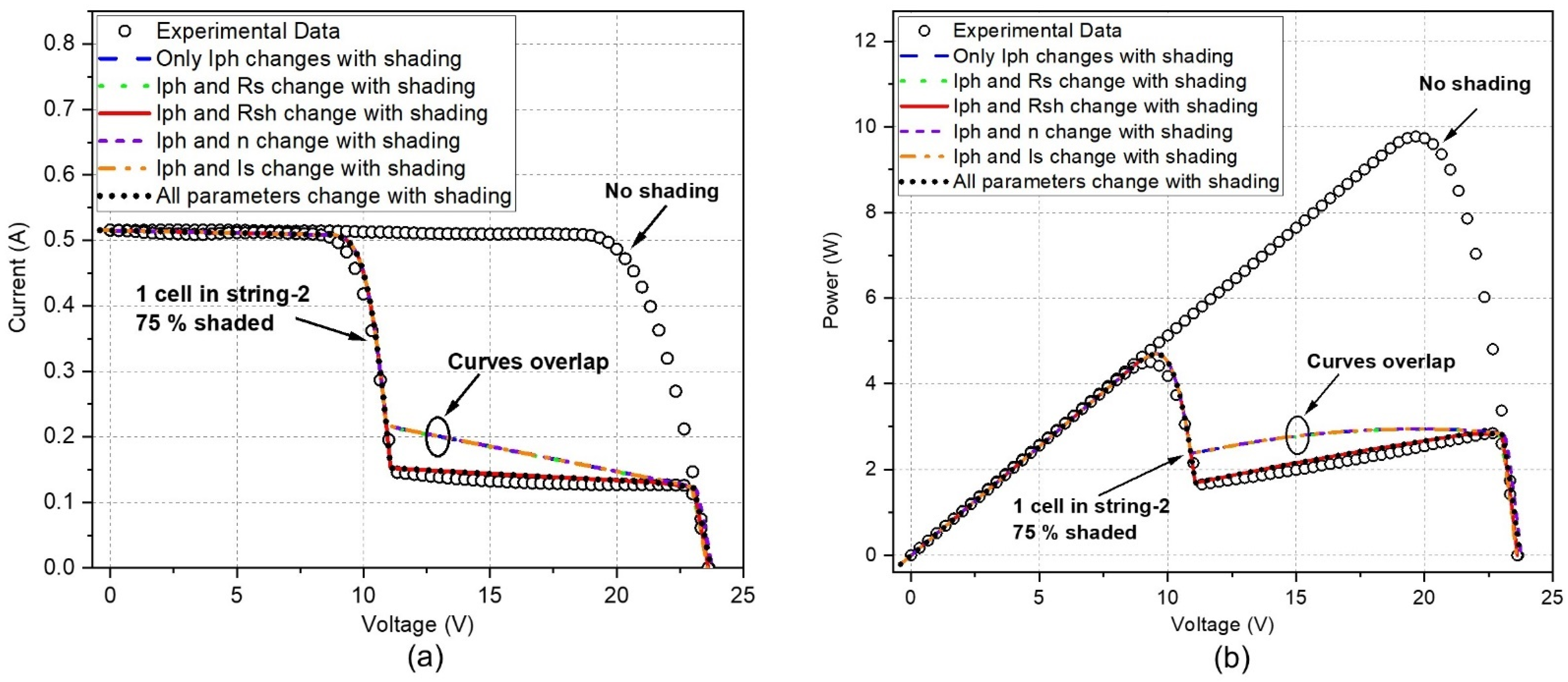
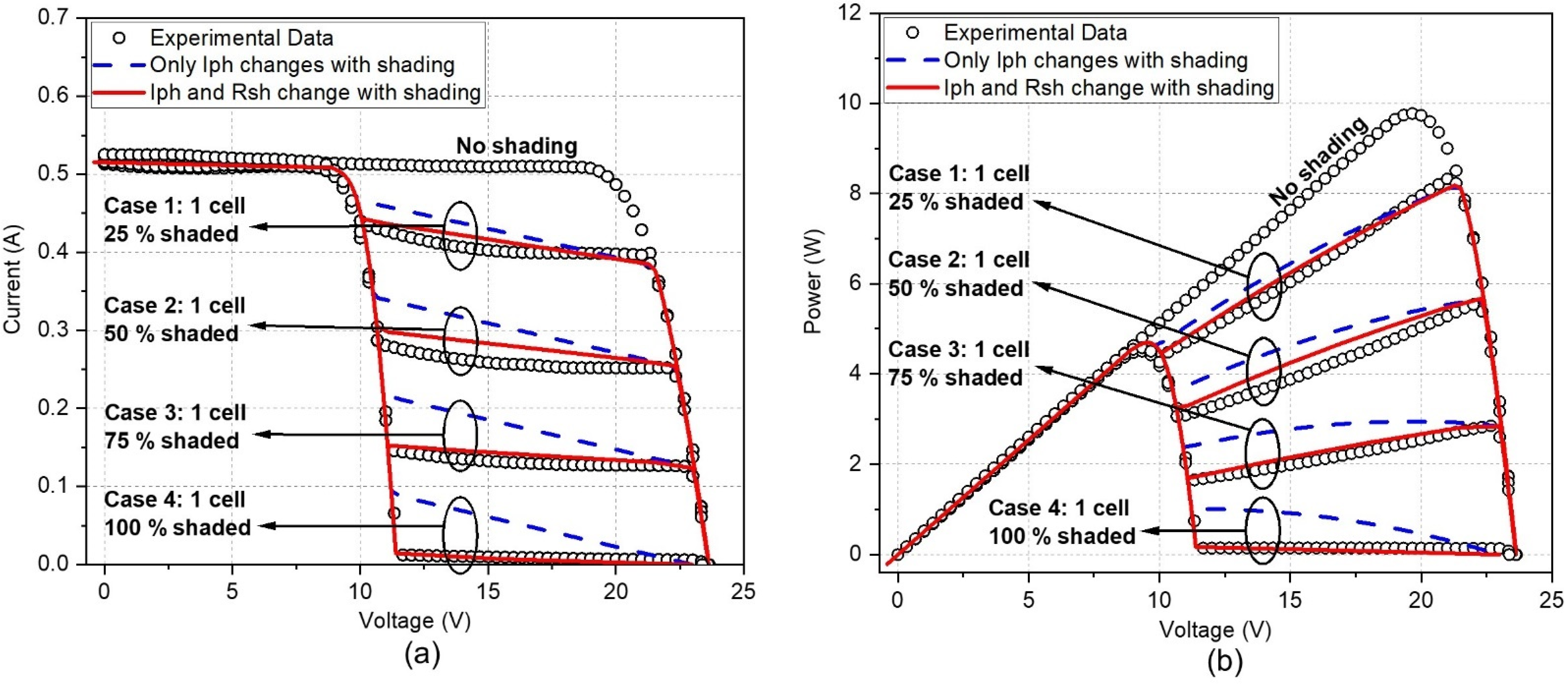
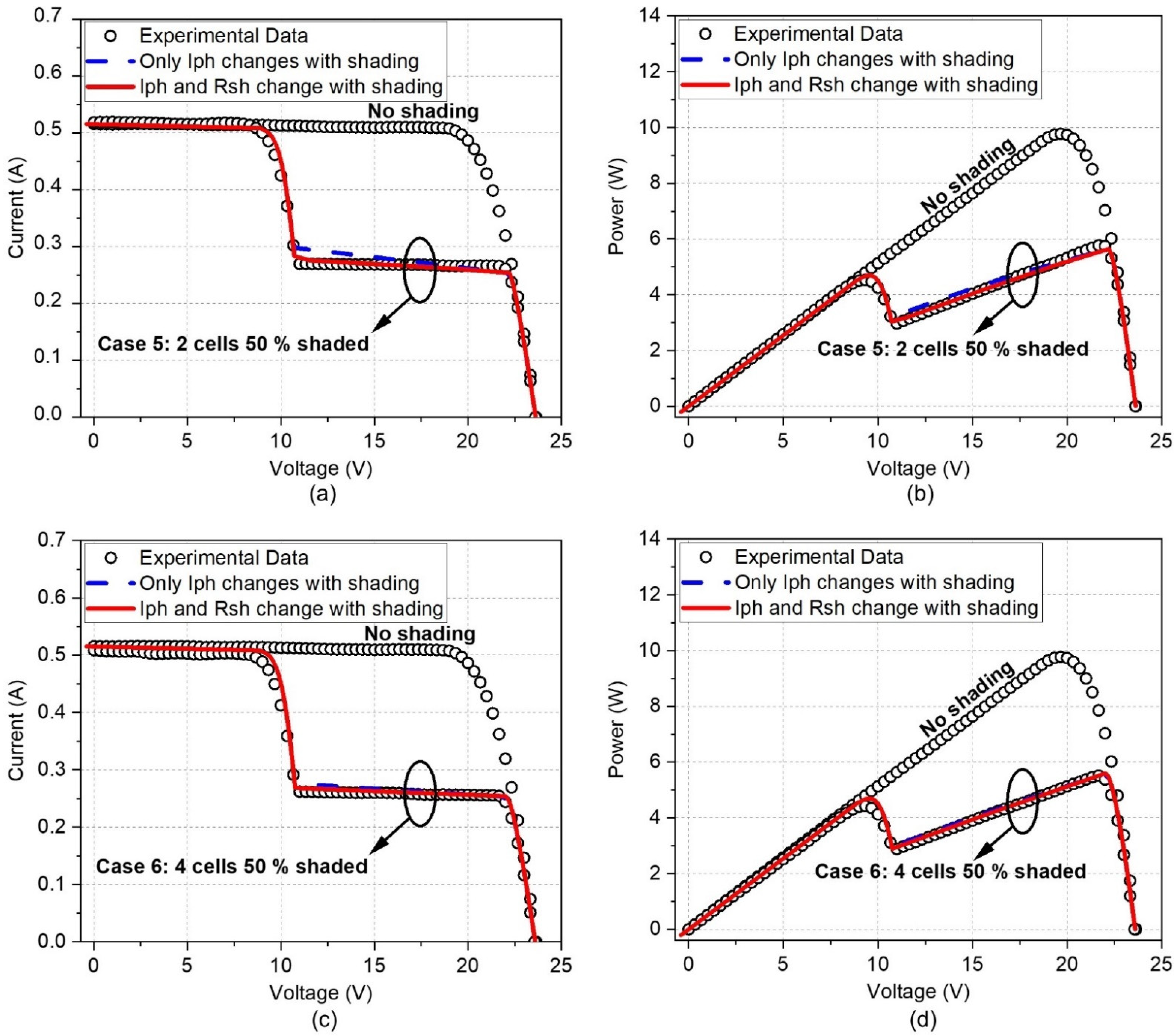
5.2. Model Considering Parameter Variation with Shading

The effect of the parameter variation with shading on the model accuracy of the PV module was investigated, by comparison with the experimental results. The model described in Section 5.1 was specifically adapted to simulate a real 10 W PV module shown in Figure 3b. Initially, the module was measured without shading to determine its P max   , I sc   and V oc   under an irradiance of 1000 W/m2, measured at the centre of the module and at a module temperature of 25 °C, which gives 9.77 W, 0.516 A and 23.643 V, respectively. The corresponding values given in the datasheet are 10 W, 0.61 A, and 21.88 V, respectively. It is to be noted that the measured short circuit ( I sc ) is almost the same as the derived photo-generated current ( I pho ), indicating the non-significance of I D and I sh   .
The equivalent circuit parameters for the PV module were determined from the measured I-V curve and the values for the individual cells were derived from the obtained module data, as listed in Table 2. The derived equivalent circuit parameters for the individual cells were then entered in the model as the initial input. Note that although   V D   of the bypass diodes (IN5819) changes with the current and temperature, it remains to be approximately 0.4 V during the experiments of this work.
For a clear comparison, the shading effect was investigated under a 75% blockage on a single cell in cell-string 2 (see Figure 3a). The precise shading was achieved by carefully positioning a black adhesive tape (see Figure 3b) on the solar cell. To identify the parameters that have a significant influence on the model accuracy, the variation of the equivalent circuit parameters described by Equations (3)–(7) was introduced into the model in the following combinations, shown in Table 3. Note that the variation of I ph was included in all cases because it is the main parameter to represent the shading influence on the performance of the solar cell. Its influence is obvious and will not be repeated in the following discussions.
The I-V and P-V curves of the PV module were calculated, based on the cases described above and the results were plotted in Figure 9a,b, respectively, together with the experimental results obtained under the same conditions. The I-V and P-V curves at the non-shading condition were also included. It can be seen that only two cases show a good fit with the experimental data. One case (black dotted line) was obtained by including the variations of all parameters and another case (red solid line) was obtained by considering the variation of   R sh   only. The other cases show a clear deviation from the experimental data in the region between 11 V and 23 V, where the shaded cell is reversely biased.
It is interesting to note that taking into account the variation of equivalent circuit parameters with shading can improve the model accuracy of the PV modules even though it has no effect on the model accuracy of a single cell (see Section 4). This finding reveals an important implication that the parameter variation, which exhibits insignificant influence at the device level, could have significant influence at the system level due to the interaction among devices. Another interesting finding from this study is that the model accuracy is mainly affected by the variation of R sh . The other parameters do not exhibit a significant effect on the model accuracy and hence their variation with shading can be neglected.

5.3. Model Considering Variation of Shunt Resistance with Shading

The model accuracy that considers the variation of R sh with shading for a different shading percentage was evaluated experimentally. The PV module used in the previous section was subjected to different shading cases, as described in Table 4. Cases 1 to 4 represent different percentages of shading imposed on a single cell, whereas case 5 and 6 represent the 50% shading imposed on two and four cells, respectively. The I-V curve for each case was obtained from the average of three measurements. All experiments were conducted under an irradiance of 1000 W/m2 measured at the centre of the module and at a module temperature of 25 °C.
The I-V curves corresponding to the above shading cases were also calculated using the model under two different assumptions. The first one was calculated by assuming that only I ph varies with shading, whereas the second one was calculated by assuming that both I ph and R sh vary with shading.
The experimental and calculated I-V and P-V curves for cases 1 to 4 are depicted in Figure 10a,b, respectively. The results show a good agreement between the calculated and experimental data over the reverse biased region for the model that considers the variation of R sh with shading. The model that considers only I ph variation (i.e., without taking into account R sh variation) exhibits significant deviation from the experimental data over the reverse biased region. Furthermore, the deviation becomes more pronounced with the increasing percentage of shading. Nevertheless, no appreciable deviation can be seen over the other regions of the I-V and P-V curves, implying that considering the variation of R sh with shading only has an impact on the reverse biased region. This observation confirms the strong correlation between R sh and the reverse bias characteristics of the solar cells reported in [8,49].
Figure 11a,b show the I-V and P-V curves for case 5 where the shading is imposed on two solar cells. Figure 11c,d show the I-V and P-V curves for case 6 where four solar cells in the same string were shaded. It can be seen that the deviation between the calculated and experimental results decreases when the number of the shaded cells is increased. The difference among the three sets of data becomes negligible when the number of the shaded cells is increased to four. This indicates that the deviation caused by neglecting the variation of R sh is only significant for the cases where the shading occurs on one cell. When the shading occurs on more than one cell, such deviation becomes negligible. This can be attributed to the fact that the breakdown voltage shifts to higher negative values when more cells are reverse biased, resulting in a flatter I–V curve in this region [7].

6. Conclusions

A systematic investigation on the partial shading of mono-Si solar cells and its impact on modelling was performed. The variation of equivalent circuit parameters with shading was determined experimentally. The results were incorporated in the models of a single solar cell and a PV module to evaluate the improvement in model accuracy. For the single solar cells, the accuracy of the model that considers the variation of all parameters with shading was compared with the model where only I ph   variation is considered. The results show that the improvement in accuracy when considering all parameters was not significant. Hence, the model that considers the variation of only I ph   is sufficient for the accurate simulation of single solar cells. For the PV modules, a significant improvement in model the accuracy was noticed when taking into account the variation of all parameters and validated experimentally using a 10 W PV module. Further study revealed that considering the variation of R sh , in addition to I ph   , played a key role for the observed improvement, compared to the case that considered the variation of I ph   only. Clearly, the results of this work suggest that in order to achieve a more accurate modelling of the PV modules, it is necessary to include the variation of both I ph   and R sh in the model for the partial shading effect.
It is interesting to note that the improvement in model accuracy of the PV modules is only significant for the case when only one cell is shaded. When the number of the cells are increased, the model that considers only the variation of I ph   can provide a similar accuracy to that considering both variations of I ph   and R sh . This result indicates that the shading of one cell in a PV module presents a unique characteristic that needs to be treated carefully, to ensure accuracy.

Author Contributions

Conceptualisation, A.A., F.A. and M.G.; methodology, A.A., F.A. and M.G.; software, A.A.; validation, A.A., F.A. and M.G.; formal analysis, A.A.; investigation, A.A. and M.G.; resources, A.A. and M.G.; data curation, A.A.; writing—original draft preparation, A.A.; writing—review and editing, A.A., F.A. and M.G.; visualisation, A.A.; supervision, F.A. and M.G.; project administration, F.A. and M.G.; funding acquisition, A.A. and M.G. All authors have read and agreed to the published version of the manuscript.

Funding

Ministry of Education in Libya for sponsoring PhD project of A.A.; EPSRC for facilities under the projects EP/K029142/1 and EPK022156/1.

Institutional Review Board Statement

Not applicable.

Informed Consent Statement

Not applicable.

Data Availability Statement

Information on the data underpinning the results presented here, including how to access them, can be found in the Cardiff University data catalogue at [10.17035/d.2022.0233852082].

Acknowledgments

A.A. acknowledges the Ministry of Education in Libya for the PhD scholarship. EPSRC is acknowledged for use of characterisation facilities of solar cells developed under the projects EP/K029142/1 and EPK022156/1. The authors would like to acknowledge the Electrical and Mechanical Workshops at Cardiff University for fabricating the PCB, heat exchanger, and solar cell test rig plate. Ali Bahr is thanked for his help in performing the calibration testing of the light source. For the purpose of open access, the author has applied CC BY public copyright licence (where permitted by UKRI, ‘Open Government Licence’ or ‘CC BY-ND public copyright licence’ may be stated instead) to Any Author Accepted Manuscript version arising.

Conflicts of Interest

The authors declare no conflict of interest.

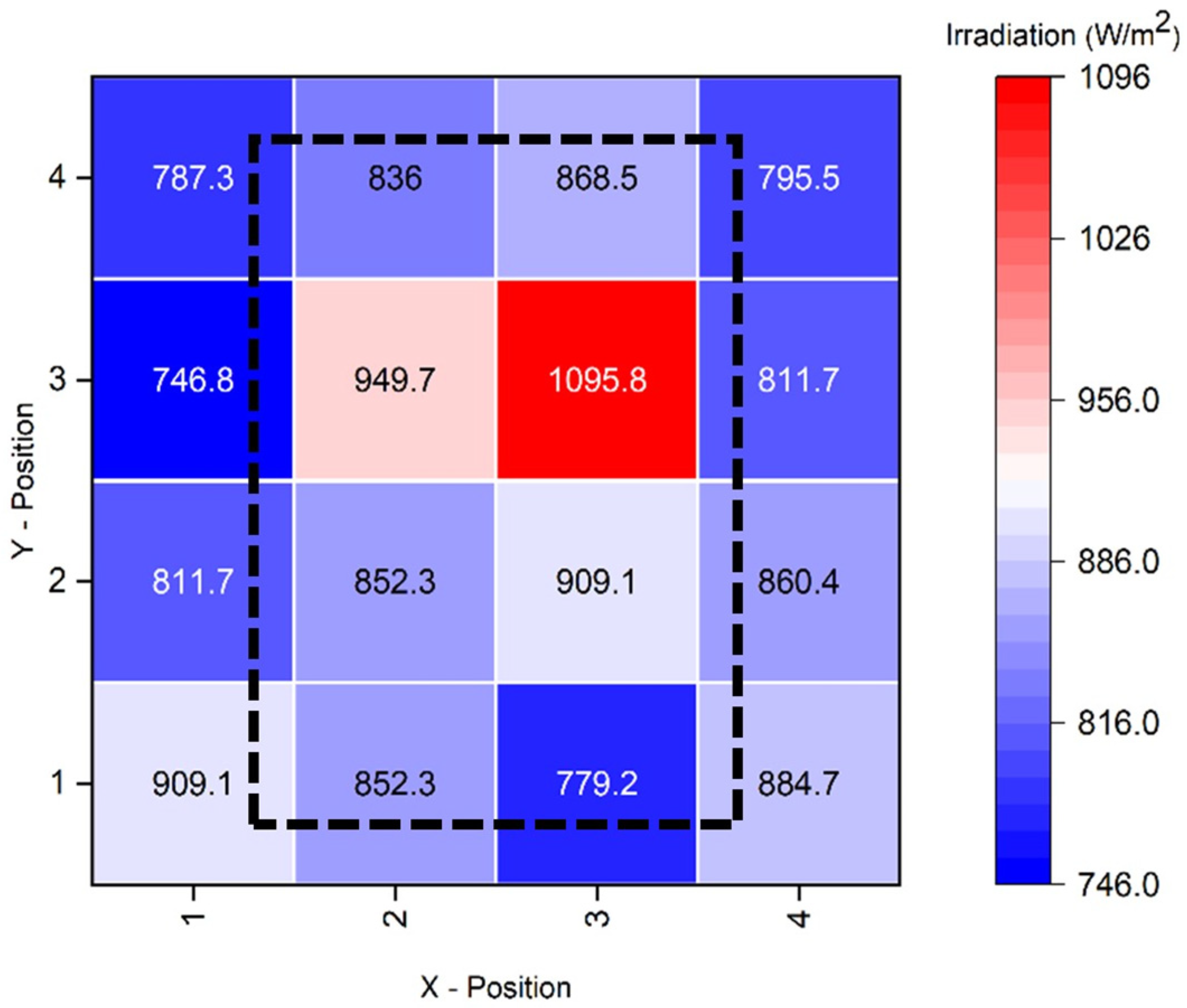
Appendix A. Determination of Spatial Non-Uniformity

Figure A1 shows the measured light intensity distribution over an area of 40 cm × 40 cm, which is divided into 16 squares of 10 cm × 10 cm. Using the data presented in Figure A1, the spatial non-uniformity was calculated using the following equation, according to the E927-10 standards:
S N = 100   %   ( G max G min ) ( G max + G min )
where S N is the spatial non-uniformity, G max and G min are the maximum and minimum irradiance levels, respectively.
Figure A1. The measured light intensity distribution over an area of 40 cm × 40 cm. The light intensity was measured using a square of 10 cm × 10 cm as a unit. The dash line box indicates that the position of the 10 W PV module during the test. The average light irradiance over the 10 W PV module is 890 W/m2 when the irradiance intensity at the centre is set at 1000 W/m2.
Energies 15 09067 g0a1

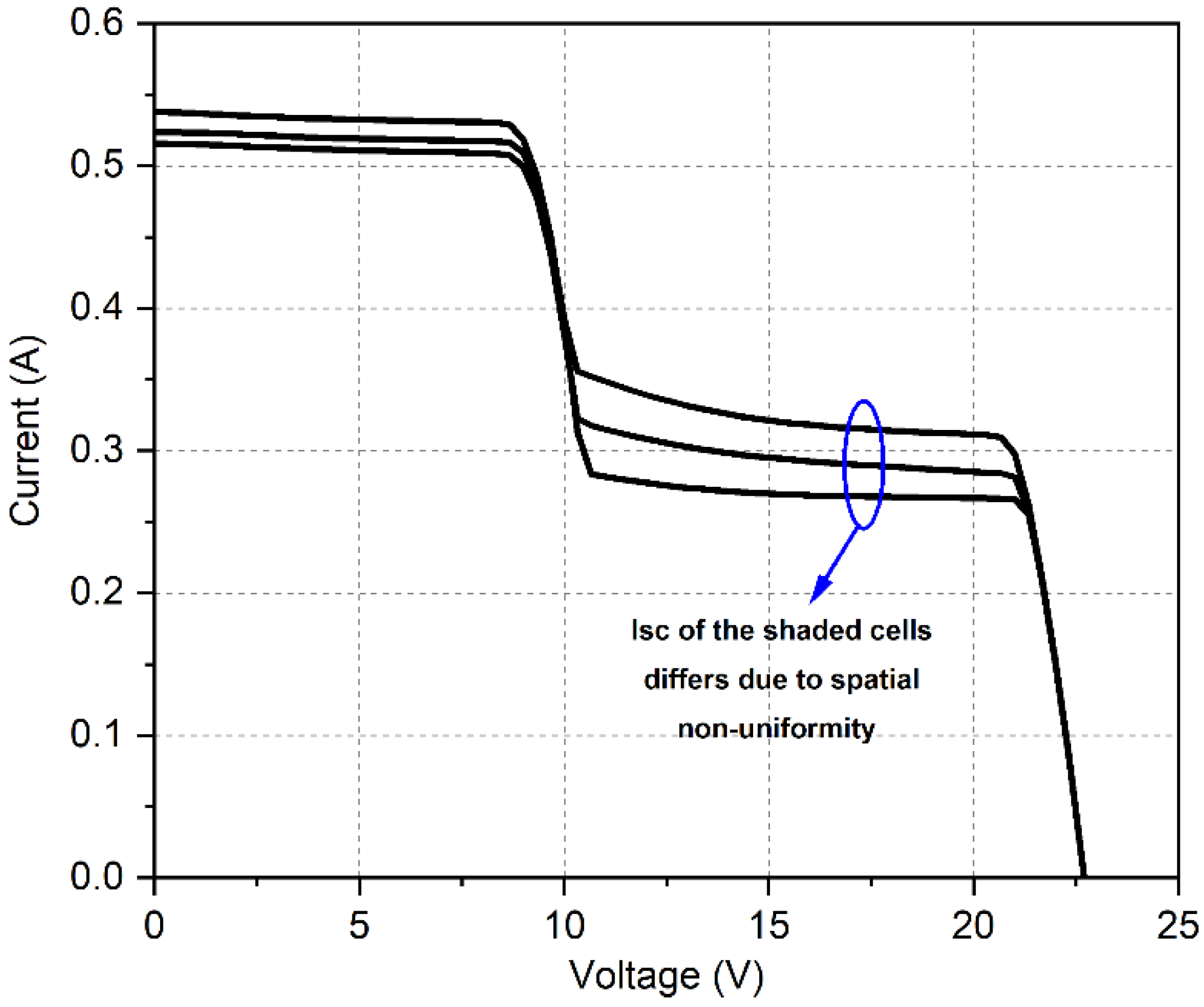
Appendix B. The Effect of the Spatial Non-Uniformity on the Shape of the I–V Curves

Figure A2 shows the I-V curves obtained from a shading experiment using the 10 W PV module placed at the centre of the 40 cm × 40 cm area (Figure A1) with an irradiance of 1000 W/m2 measured at the centre of the module, where the 50% of a solar cell was blocked. The experiment was repeated by blocking each of the three different solar cells, respectively. It can be seen that the three curves are not overlapped with each other. Instead, they appear to show a shift along the vertical axis. This is due to the fact that the light intensity received by these three cells are different, due to the non-uniformity of the light source (see Figure A1). It is to be noted that the shape of the three curves remains approximately the same, except for the vertical shift. This result indicates that the non-uniformity of the light source causes a shift on the I-V curves but it has no significant effect on the slopes of the I-V curves. As the key focus of this study is related to the investigation and understanding of the slope change of the I-V curves (as shown in Figure 9), the results of Figure A2 demonstrate that the non-uniformity of the light source has no effect on the validity of this study.
Figure A2. I-V curves of the 10 W PV module under 50% shading of three different cells. The figure shows that the spatial non-uniformity affects only the current of the shaded cell represented in the height of the horizontal part between about 11 and 21 V. It does not significantly affect the shape of the I-V curve. Each I-V curve is the average of three measurements under a light irradiance of 1000 W/m2 measured at the centre of the module at a module temperature of 40 °C.
Energies 15 09067 g0a2

References

  1. Quaschning, V. Understanding Renewable Energy Systems, Technology and Practice, 1st ed.; Earthscan: London, UK, 2005. [Google Scholar]
  2. Mertens, K. Photovoltaics Fundamentals, Technology and Practice; Wiley: Chichester, UK, 2014. [Google Scholar]
  3. Dhimish, M.; Holmes, V.; Mather, P.; Sibley, M. Novel Hot Spot Mitigation Technique to Enhance Photovoltaic Solar Panels Output Power Performance. Sol. Energy Mater. Sol. Cells 2018, 179, 72–79. [Google Scholar] [CrossRef] [Green Version]
  4. Batzelis, E.I.; Georgilakis, P.S.; Papathanassiou, S.A. Energy Models for Photovoltaic Systems under Partial Shading Conditions: A Comprehensive Review. IET Renew. Power Gener. 2015, 9, 340–349. [Google Scholar] [CrossRef]
  5. Ishaque, K.; Salam, Z.; Syafaruddin. A Comprehensive MATLAB Simulink PV System Simulator with Partial Shading Capability Based on Two-Diode Model. Sol. Energy 2011, 85, 2217–2227. [Google Scholar] [CrossRef]
  6. Bishop, J.W. Computer Simulation of the Effects of Electrical Mismatches in Photovoltaic Cell Interconnection Circuits. Sol. Cells 1988, 25, 73–89. [Google Scholar] [CrossRef]
  7. Kawamura, H.; Naka, K.; Yonekura, N.; Yamanaka, S.; Kawamura, H.; Ohno, H.; Naito, K. Simulation of I-V Characteristics of a PV Module with Shaded PV Cells. Sol. Energy Mater. Sol. Cells 2003, 75, 613–621. [Google Scholar] [CrossRef]
  8. Alonso-García, M.C.; Ruiz, J.M.; Herrmann, W. Computer Simulation of Shading Effects in Photovoltaic Arrays. Renew. Energy 2006, 31, 1986–1993. [Google Scholar] [CrossRef]
  9. Karatepe, E.; Boztepe, M.; Çolak, M. Development of a Suitable Model for Characterizing Photovoltaic Arrays with Shaded Solar Cells. Sol. Energy 2007, 81, 977–992. [Google Scholar] [CrossRef]
  10. Silvestre, S.; Chouder, A. Effects of Shadowing on Photovoltaic Module Performance. Prog. Photovolt. Res. Appl. 2008, 16, 141–149. [Google Scholar] [CrossRef]
  11. Patel, H.; Agarwal, V. MATLAB-Based Modeling to Study the Effects of Partial Shading on PV Array Characteristics. IEEE Trans. Energy Convers. 2008, 23, 302–310. [Google Scholar] [CrossRef]
  12. Wang, Y.J.; Hsu, P.C. Analytical Modelling of Partial Shading and Different Orientation of Photovoltaic Modules. IET Renew. Power Gener. 2010, 4, 272–282. [Google Scholar] [CrossRef]
  13. Picault, D.; Raison, B.; Bacha, S.; de la Casa, J.; Aguilera, J. Forecasting Photovoltaic Array Power Production Subject to Mismatch Losses. Sol. Energy 2010, 84, 1301–1309. [Google Scholar] [CrossRef]
  14. Moballegh, S.; Jiang, J. Partial Shading Modeling of Photovoltaic System with Experimental Validations. In Proceedings of the 2011 IEEE Power and Energy Society General Meeting, Detroit, MI, USA, 24–28 July 2011; IEEE: Piscataway, NJ, USA, 2011; pp. 1–9. [Google Scholar] [CrossRef]
  15. Seyedmahmoudian, M.; Mekhilef, S.; Rahmani, R.; Yusof, R.; Renani, E.T. Analytical Modeling of Partially Shaded Photovoltaic Systems. Energies 2013, 6, 128–144. [Google Scholar] [CrossRef] [Green Version]
  16. Jung, T.H.; Ko, J.W.; Kang, G.H.; Ahn, H.K. Output Characteristics of PV Module Considering Partially Reverse Biased Conditions. Sol. Energy 2013, 92, 214–220. [Google Scholar] [CrossRef]
  17. Orozco-Gutierrez, M.L.; Ramirez-Scarpetta, J.M.; Spagnuolo, G.; Ramos-Paja, C.A. A Technique for Mismatched PV Array Simulation. Renew. Energy 2013, 55, 417–427. [Google Scholar] [CrossRef]
  18. Olalla, C.; Clement, D.; Maksimovic, D.; Deline, C. A Cell-Level Photovoltaic Model for High-Granularity Simulations. In Proceedings of the 2013 15th European Conference on Power Electronics and Applications (EPE), Lille, France, 2–6 September 2013; IEEE: Piscataway, NJ, USA, 2013; pp. 1–10. [Google Scholar] [CrossRef]
  19. Batzelis, E.I.; Routsolias, I.A.; Papathanassiou, S.A. An Explicit PV String Model Based on the Lambert W Function and Simplified MPP Expressions for Operation under Partial Shading. IEEE Trans Sustain. Energy 2014, 5, 301–312. [Google Scholar] [CrossRef]
  20. Wang, Y.; Pei, G.; Zhang, L. Effects of Frame Shadow on the PV Character of a Photovoltaic/Thermal System. Appl. Energy 2014, 130, 326–332. [Google Scholar] [CrossRef]
  21. Bai, J.; Cao, Y.; Hao, Y.; Zhang, Z.; Liu, S.; Cao, F. Characteristic Output of PV Systems under Partial Shading or Mismatch Conditions. Sol. Energy 2015, 112, 41–54. [Google Scholar] [CrossRef]
  22. Psarros, G.N.; Batzelis, E.I.; Papathanassiou, S.A. Partial Shading Analysis of Multistring PV Arrays and Derivation of Simplified MPP Expressions. IEEE Trans Sustain. Energy 2015, 6, 499–508. [Google Scholar] [CrossRef]
  23. Qing, X.; Sun, H.; Feng, X.; Chung, C.Y. Submodule-Based Modeling and Simulation of a Series-Parallel Photovoltaic Array under Mismatch Conditions. IEEE J. Photovolt. 2017, 7, 1731–1739. [Google Scholar] [CrossRef]
  24. Torres, J.P.N.; Nashih, S.K.; Fernandes, C.A.F.; Leite, J.C. The Effect of Shading on Photovoltaic Solar Panels. Energy Syst. 2018, 9, 195–208. [Google Scholar] [CrossRef]
  25. Galeano, A.G.; Bressan, M.; Vargas, F.J.; Alonso, C. Shading Ratio Impact on Photovoltaic Modules and Correlation with Shading Patterns. Energies 2018, 11, 852. [Google Scholar] [CrossRef] [Green Version]
  26. Zhu, L.; Li, Q.; Chen, M.; Cao, K.; Sun, Y. A Simplified Mathematical Model for Power Output Predicting of Building Integrated Photovoltaic under Partial Shading Conditions. Energy Convers. Manag. 2019, 180, 831–843. [Google Scholar] [CrossRef]
  27. Bharadwaj, P.; John, V. Subcell Modeling of Partially Shaded Photovoltaic Modules. IEEE Trans. Ind. Appl. 2019, 55, 3046–3054. [Google Scholar] [CrossRef]
  28. Ding, K.; Bian, X.; Liu, H.; Peng, T. A MATLAB-Simulink-Based PV Module Model and Its Application under Conditions of Nonuniform Irradiance. IEEE Trans. Energy Convers. 2012, 27, 864–872. [Google Scholar] [CrossRef]
  29. Quaschning, V.; Hanitsch, R. Numerical Simulation of Current-Voltage Characteristics of Photovoltaic Systems with Shaded Solar Cells. Sol. Energy 1996, 56, 513–520. [Google Scholar] [CrossRef]
  30. Ishaque, K.; Salam, Z.; Taheri, H.; Syafaruddin. Modeling and Simulation of Photovoltaic (PV) System during Partial Shading Based on a Two-Diode Model. Simul. Model. Pract. Theory 2011, 19, 1613–1626. [Google Scholar] [CrossRef]
  31. Silvestre, S.; Boronat, A.; Chouder, A. Study of Bypass Diodes Configuration on PV Modules. Appl. Energy 2009, 86, 1632–1640. [Google Scholar] [CrossRef]
  32. Paraskevadaki, E.V.; Papathanassiou, S.A. Evaluation of MPP Voltage and Power of Mc-Si PV Modules in Partial Shading Conditions. IEEE Trans. Energy Convers. 2011, 26, 923–932. [Google Scholar] [CrossRef]
  33. Zegaoui, A.; Petit, P.; Aillerie, M.; Sawicki, J.P.; Belarbi, A.W.; Krachai, M.D.; Charles, J.P. Photovoltaic Cell/Panel/Array Characterizations and Modeling Considering Both Reverse and Direct Modes. Energy Procedia 2011, 6, 695–703. [Google Scholar] [CrossRef]
  34. Di Vincenzo, M.C.; Infield, D. Detailed PV Array Model for Non-Uniform Irradiance and Its Validation against Experimental Data. Sol. Energy 2013, 97, 314–331. [Google Scholar] [CrossRef]
  35. Kermadi, M.; Chin, V.J.; Mekhilef, S.; Salam, Z. A Fast and Accurate Generalized Analytical Approach for PV Arrays Modeling under Partial Shading Conditions. Sol. Energy 2020, 208, 753–765. [Google Scholar] [CrossRef]
  36. Villalva, M.G.; Gazoli, J.R.; Filho, E.R. Comprehensive Approach to Modeling and Simulation of Photovoltaic Arrays. IEEE Trans. Power Electron. 2009, 24, 1198–1208. [Google Scholar] [CrossRef]
  37. Herrmann, W.; Wiesner, W.; Vaassen, W. Hot Spot Investigations on PV Modules—New Concepts for a Test Standard and Consequences for Module Design with Respect to Bypass Diodes. In Proceedings of the Conference Record of the Twenty Sixth IEEE Photovoltaic Specialists Conference, Anaheim, CA, USA, 29 September–3 October 1997; IEEE: Piscataway, NJ, USA, 1997; pp. 1129–1132. [Google Scholar] [CrossRef]
  38. Alonso-García, M.C.; Ruíz, J.M. Analysis and Modelling the Reverse Characteristic of Photovoltaic Cells. Sol. Energy Mater. Sol. Cells 2006, 90, 1105–1120. [Google Scholar] [CrossRef]
  39. Al-Shidhani, M.; Al-Najideen, M.; Rocha, V.G.; Min, G. Design and Testing of 3D Printed Cross Compound Parabolic Concentrators for LCPV System. In AIP Conference Proceedings; American Institute of Physics Inc.: College Park, MD, USA, 2018; Volume 2012, pp. 020001-1–020001-8. [Google Scholar] [CrossRef]
  40. Atia, A.; Anayi, F.; Min, G. Improving Accuracy of Solar Cells Parameters Extraction by Minimum Root Mean Square Error. In Proceedings of the 2020 55th International Universities Power Engineering Conference (UPEC), Turin, Italy, 1–4 September 2020; IEEE: Piscataway, NJ, USA, 2020; pp. 1–6. [Google Scholar] [CrossRef]
  41. Phang, J.C.H.; Chan, D.S.H.; Phillips, J.R. Accurate Analytical Method for the Extraction of Solar Cell Model Parameters. Electron. Lett. 1984, 20, 406–408. [Google Scholar] [CrossRef]
  42. Duffie, J.A.; Beckman, W.A. Solar Engineering of Thermal Processes, 4th ed.; Wiley: Hoboken, NJ, USA, 2013. [Google Scholar]
  43. Khan, F.; Singh, S.N.; Husain, M. Effect of Illumination Intensity on Cell Parameters of a Silicon Solar Cell. Sol. Energy Mater. Sol. Cells 2010, 94, 1473–1476. [Google Scholar] [CrossRef]
  44. Atia, A.; Anayi, F.; Min, G. Comparing Shading with Irradiance Reduction Effects on Solar Cells Electrical Parameters. In Proceedings of the 2021 56th International Universities Power Engineering Conference (UPEC), Middlesbrough, UK, 31 August–3 September 2021; IEEE: Piscataway, NJ, USA, 2021; pp. 1–5. [Google Scholar] [CrossRef]
  45. De Soto, W.; Klein, S.A.; Beckman, W.A. Improvement and Validation of a Model for Photovoltaic Array Performance. Sol. Energy 2006, 80, 78–88. [Google Scholar] [CrossRef]
  46. Ruschel, C.S.; Gasparin, F.P.; Costa, E.R.; Krenzinger, A. Assessment of PV Modules Shunt Resistance Dependence on Solar Irradiance. Sol. Energy 2016, 133, 35–43. [Google Scholar] [CrossRef]
  47. Villalva, M.G. Modeling and Simulation of Photovoltaic Arrays. Sites. Available online: https://sites.google.com/site/mvillalva/pvmodel (accessed on 16 February 2022).
  48. Tian, H.; Mancilla-David, F.; Ellis, K.; Muljadi, E.; Jenkins, P. A Cell-to-Module-to-Array Detailed Model for Photovoltaic Panels. Sol. Energy 2012, 86, 2695–2706. [Google Scholar] [CrossRef]
  49. Meyer, E.L.; van Dyk, E.E. The Effect of Reduced Shunt Resistance and Shading on Photovoltaic Module Performance. In Proceedings of the Conference Record of the Thirty-first IEEE Photovoltaic Specialists Conference, Lake Buena Vista, FL, USA, 3–7 January 2005; IEEE: Piscataway, NJ, USA, USA, 2005; pp. 1331–1334. [Google Scholar] [CrossRef]
Figure 1. Single diode five-parameter model of a solar cell. (Adapted from [1,2]).
Energies 15 09067 g001
Figure 2. The solar cell testing assembly with the water-cooling system, showing the cell under light irradiation and partial shading.
Energies 15 09067 g002
Figure 3. The 10 W PV module: (a) The configuration of the cells and bypass diodes. The blue box represents cell-string 1 and the red box represent cell-string 2. (b) The module testing assembly connected to the water cooling and under shading experiments.
Energies 15 09067 g003
Figure 4. The facility for the characterisation of the solar cells and PV modules.
Energies 15 09067 g004
Figure 5. The variation of the equivalent circuit parameters with shading: (a) Series resistance; (b) Shunt resistance; (c) Ideality factor; (d) Reverse saturation current; (e) Photo-generated current. Each data point in the figures represents the average value of the data extracted from two I-V curves with each I-V curve formed using the average of three measurements. The error bars were determined from 12 measurements taken without shading in STCs.
Energies 15 09067 g005
Figure 6. The variation of the performance parameters with shading: (a) Maximum power; (b) Short circuit current; (c) Open circuit voltage; (d) Fill factor; (e) Efficiency; (f) Characteristics resistance. Each data point in the figures represents the average value of the data extracted from two I-V curves with each I-V curve formed using the average of three measurements. The error bars were determined from 12 measurements taken without shading in STCs.
Energies 15 09067 g006
Figure 7. Experimental and calculated I-V and P-V curves of the solar cell under different shading. The black circles are experimental results. The red solid lines represent the calculated results that consider the variation of all parameters with shading. The blue dashed lines represent the calculated results that consider the variation of I ph   only: (a) I-V curves; (b) P-V curves. Each experimental curve is the average of three measurements under a light irradiance of 1000 W/m2 at a cell temperature of 25 °C.
Energies 15 09067 g007
Figure 8. A configuration of a PV module shown as an example to illustrate the voltage calculations. The module consists of a total of s strings with each string consist of c solar cells.
Energies 15 09067 g008
Figure 9. Experimental and calculated I-V and P-V curves of the 10 W PV module at the non-shading and under 75% of shading on a single cell. The simulation was carried out by considering the parameter variation with shading for six cases listed in Table 3: (a) I-V curves; (b) P-V curves. Each experimental curve is the average of three measurements under a light irradiance of 1000 W/m2 measured at the centre of the module at a module temperature of 25 °C.
Energies 15 09067 g009
Figure 10. Experimental and calculated I-V and P-V curves of the 10 W PV module for cases 1 to 4. The black circles are the experimental results. The red solid lines represent the calculated results that consider the variation of both I ph   and R sh   . The blue dashed lines represent the calculated results that consider the variation of Iph only: (a) I-V curves; (b) P-V curves. Each experimental curve is the average of three measurements under a light irradiance of 1000 W/m2 measured at the centre of the module at a module temperature of 25 °C.
Energies 15 09067 g010
Figure 11. Experimental and calculated I-V and P-V curves of the 10 W PV module for cases 5 and 6. The black circles are experimental results. The red solid lines represent the calculated results that consider the variations of both I ph   and R sh   . The blue dashed lines represent the calculated results that consider the variation of I ph   only: (a) I-V curve of case 5; (b) P-V curve of case 5; (c) I-V curve of case 6; (d) P-V curve of case 6. Each experimental curve is the average of three measurements under a light irradiance of 1000 W/m2 measured at the centre of the module at a module temperature of 25 °C.
Energies 15 09067 g011
Table 1. The equivalent circuit parameters of the solar cell (0.8 cm2 active area) in STCs. They were used as the non-shading reference in the model for the calculation of the shading influence. The data was extracted from an I-V curve obtained from the average of three measurements.
ParameterNon-Shading Value in STCs
R so (Ω)0.80
R sho (kΩ)0.36
n o 2.05
  I so (µA)0.47
I pho (mA)27.85
Table 2. The equivalent circuit parameters of the 10 W PV module under an irradiance of 1000 W/m2 measured at the centre of the module and at a module temperature of 25 °C. The series and shunt resistances for the individual cells were obtained by dividing R so and R sho by the number of cells. The parameters of the individual cells were used as the non-shading reference in the model for calculation of the shading influence. The data was extracted from the experimental I-V curve, based on the average of three measurements.
ParameterNon-Shading Value in STCs for PV ModuleNon-Shading Value in STCs for Individual Cells
R so (Ω)3.05 0.085
R sho (kΩ)4.5 0.125
n o 0.74 0.74
  I so (nA)6 × 10⁻⁷ 6 × 10⁻⁷
I pho (A)0.516 0.516
Table 3. Cases for considering the parameter variation with shading in the modelling of the 10 W PV module.
CaseParameters Considered
1Only I ph
2 I ph and R s
3 I ph and R sh
4 I ph and n
5 I ph and I s
6All five parameters
Table 4. The shading cases imposed on a 10 W PV module, consisting of two strings with 18 solar cells in each string.
Shading CaseCell-String 1Cell-String 2
1No shading1 cell 25% shading
2No shading1 cell 50% shading
3No shading1 cell 75% shading
4No shading1 cell 100% shading
5No shading2 cells 50% shading
6No shading4 cells 50% shading
Publisher’s Note: MDPI stays neutral with regard to jurisdictional claims in published maps and institutional affiliations.

