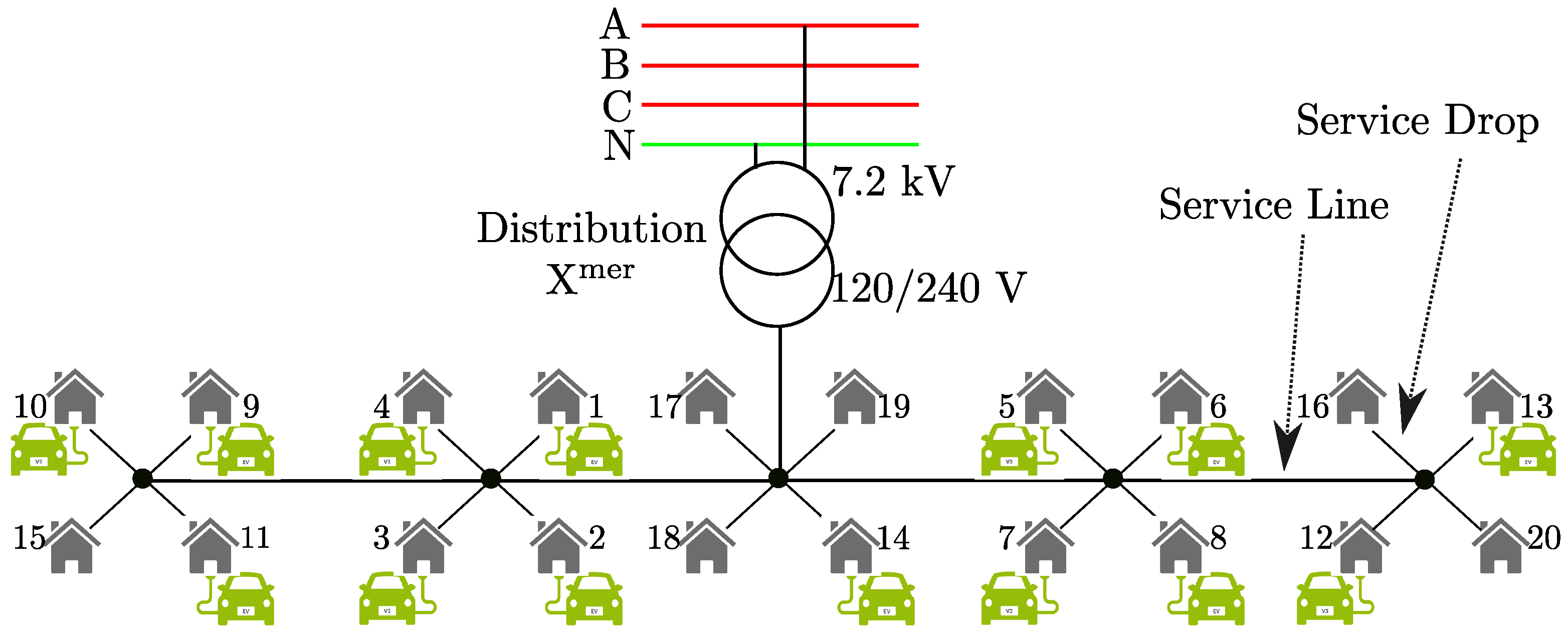
Figure 1.
Schematic of secondary distribution system used for this study.
Figure 1.
Schematic of secondary distribution system used for this study.
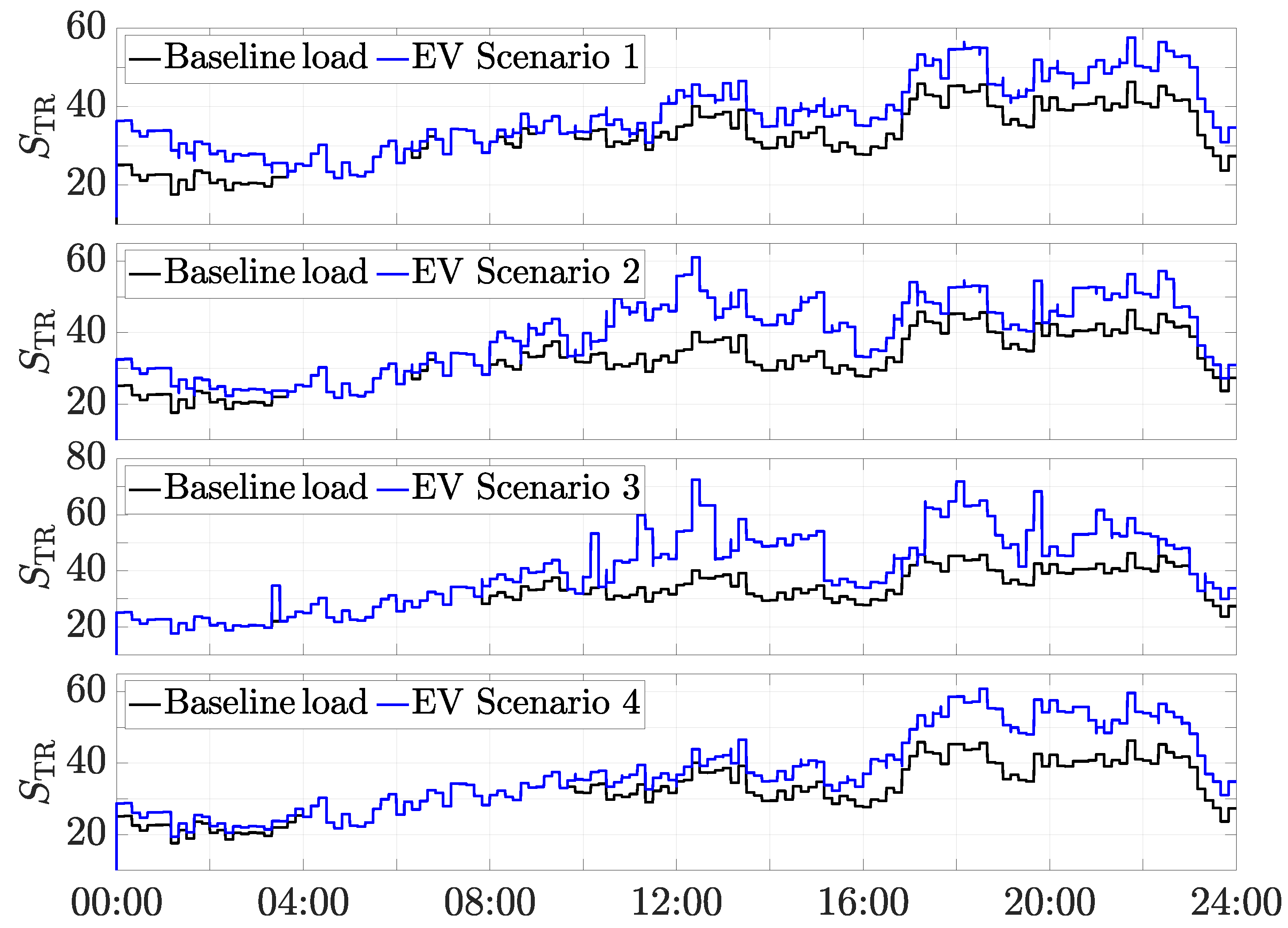
Figure 2.
Transformer loading under different EV charging scenarios ( in kVA).
Figure 2.
Transformer loading under different EV charging scenarios ( in kVA).
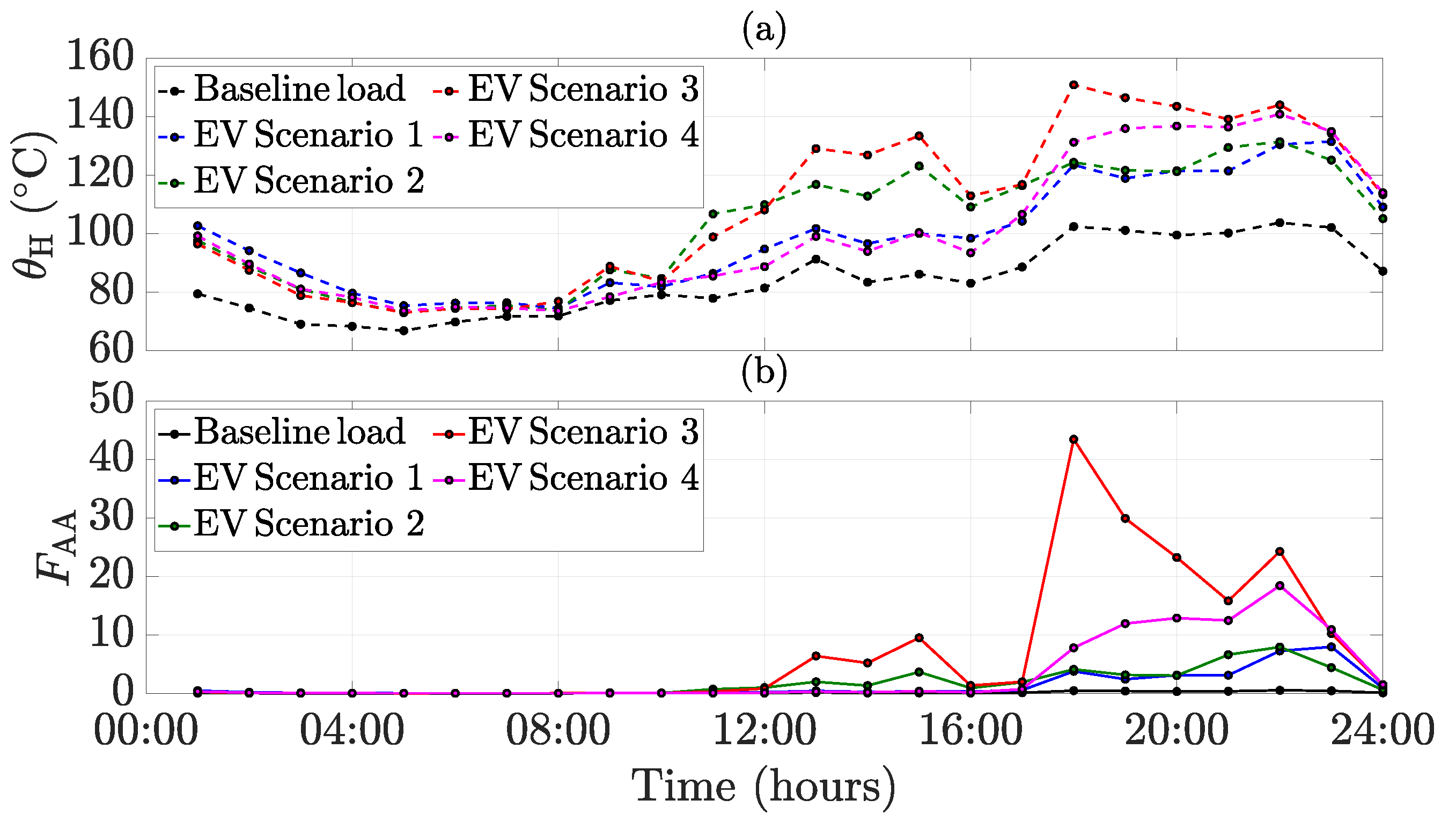
Figure 3.
Transformer life indices without EV and with EV charging, (a) hottest-spot temperature, ; (b) accelerated aging factor, .
Figure 3.
Transformer life indices without EV and with EV charging, (a) hottest-spot temperature, ; (b) accelerated aging factor, .
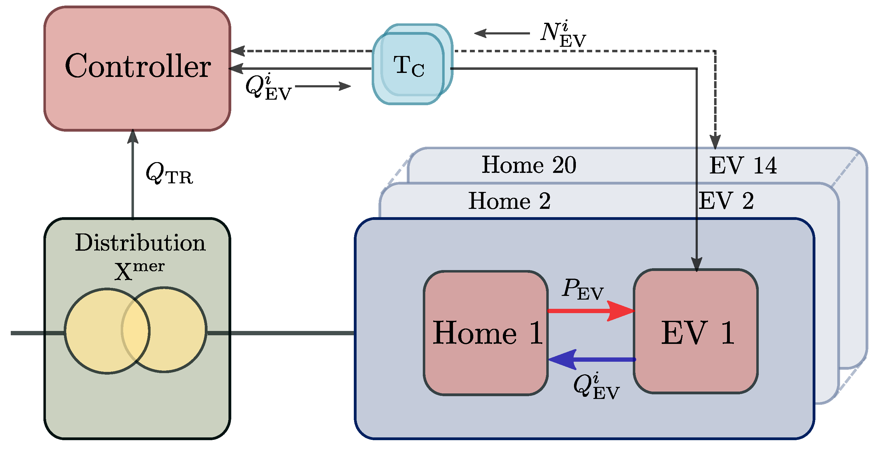
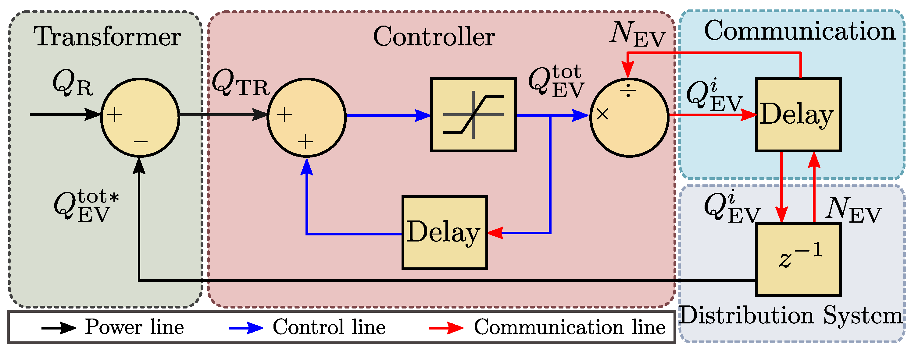
Figure 4.
Entire system’s block diagram.
Figure 4.
Entire system’s block diagram.
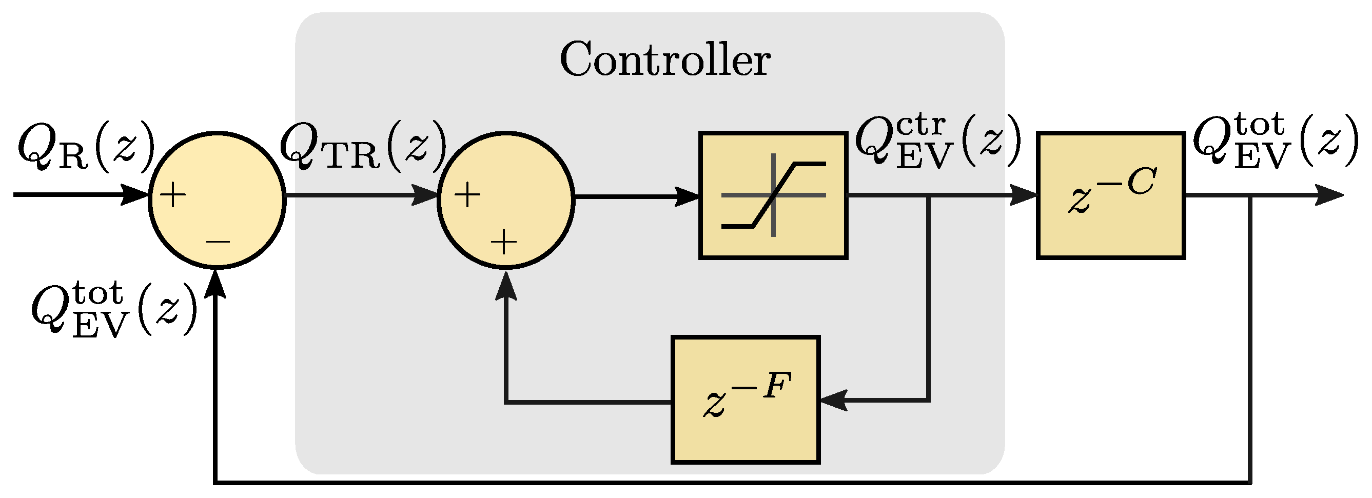
Figure 5.
Simplified system and controller model.
Figure 5.
Simplified system and controller model.
Figure 6.
Simplified system and controller model for stability analysis.
Figure 6.
Simplified system and controller model for stability analysis.
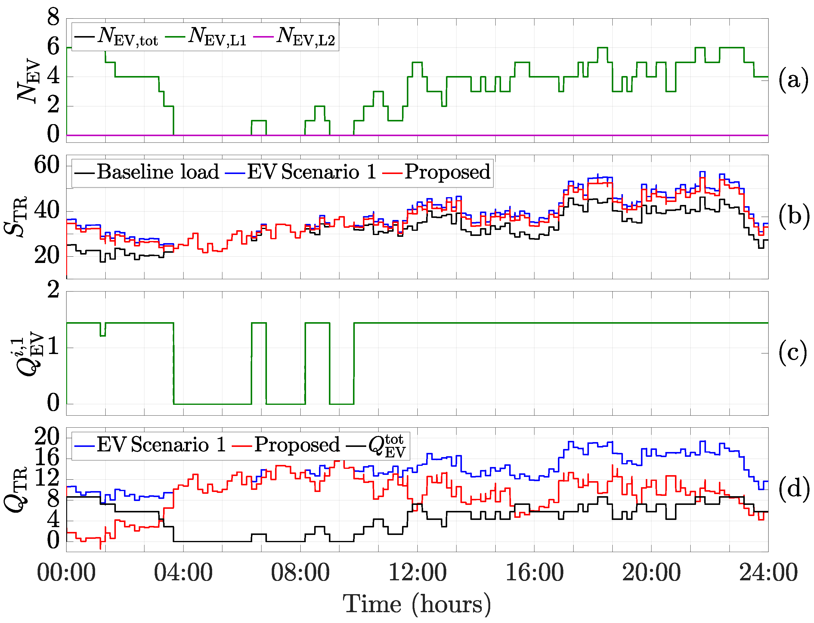
Figure 7.
Scenario 1: EV charging at Level 1, (a) number of EVs present; (b) transformer apparent power in kVA; (c) Q supplied by an online EV at Level 1 in kVAr; (d) transformer reactive power in kVAr.
Figure 7.
Scenario 1: EV charging at Level 1, (a) number of EVs present; (b) transformer apparent power in kVA; (c) Q supplied by an online EV at Level 1 in kVAr; (d) transformer reactive power in kVAr.
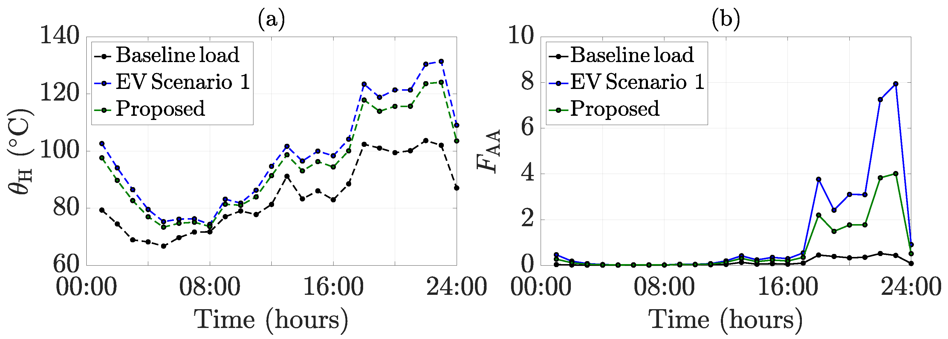
Figure 8.
Transformer life indices in scenario 1, (a) hottest-spot temperature, ; (b) accelerated aging factor, .
Figure 8.
Transformer life indices in scenario 1, (a) hottest-spot temperature, ; (b) accelerated aging factor, .
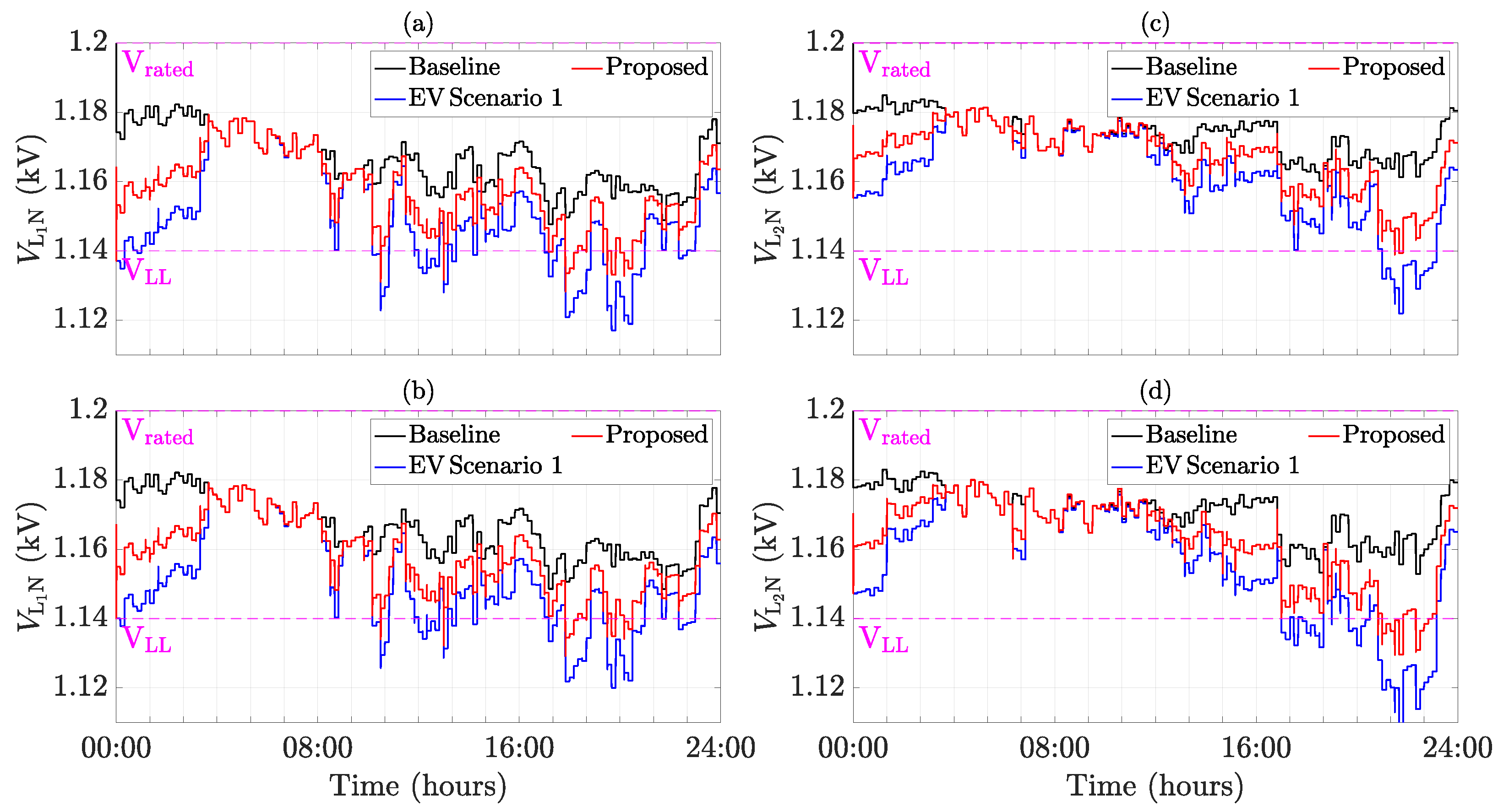
Figure 9.
Phase voltages in scenario 1, (a) at bus 10 with EV charging between phase ; (b) at bus 15 with no EV present at it; (c) at bus 8 with EV charging between phase ; (d) at bus 13 with EV charging between phase .
Figure 9.
Phase voltages in scenario 1, (a) at bus 10 with EV charging between phase ; (b) at bus 15 with no EV present at it; (c) at bus 8 with EV charging between phase ; (d) at bus 13 with EV charging between phase .
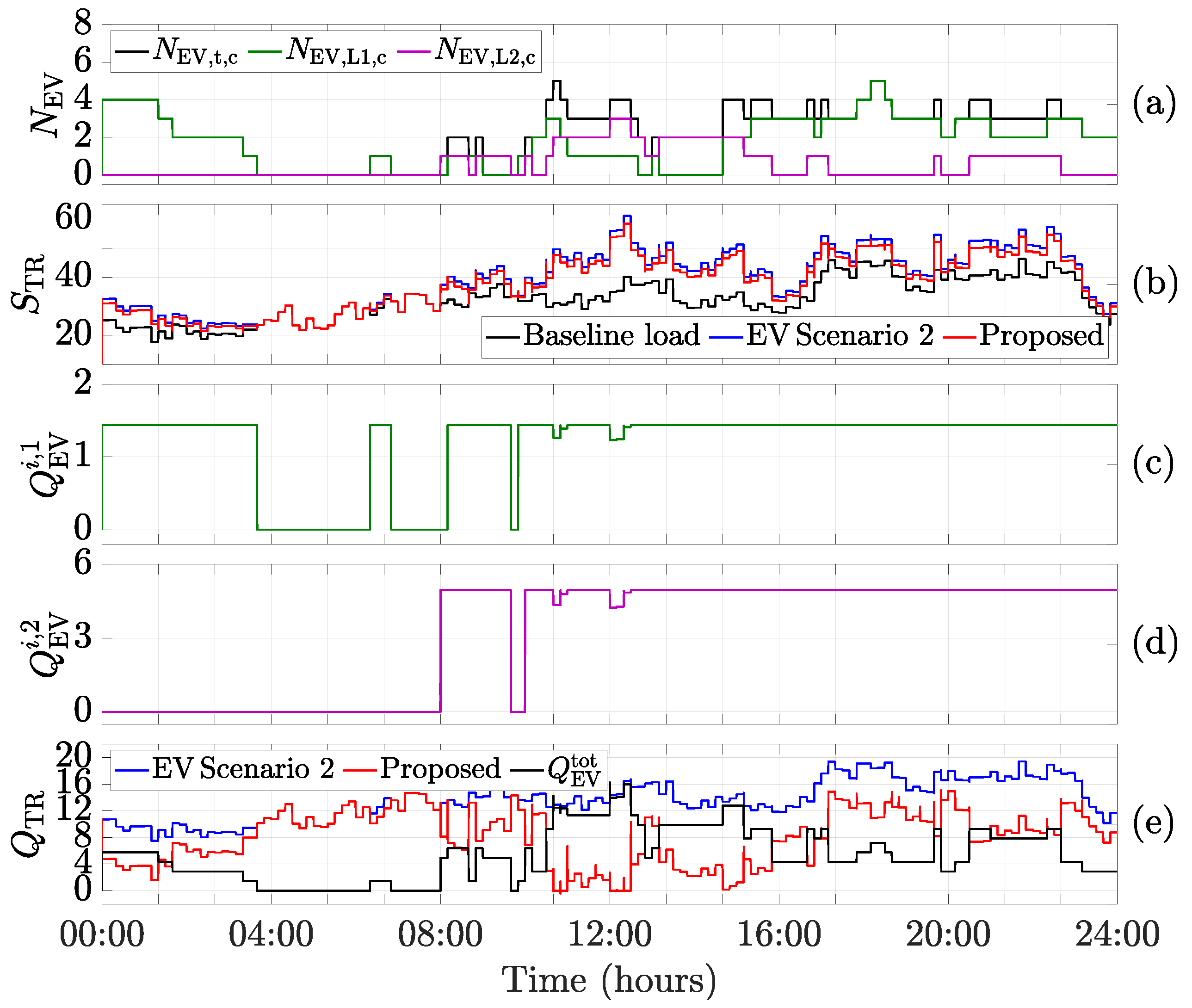
Figure 10.
Scenario 2: combined Level 1 and Level 2, (a) number of EVs present; (b) transformer apparent power in kVA; (c) Q supplied by an online EV at Level 1 in kVAr; (d) Q supplied by an online EV at Level 2 in kVAr; (e) transformer reactive power in kVAr.
Figure 10.
Scenario 2: combined Level 1 and Level 2, (a) number of EVs present; (b) transformer apparent power in kVA; (c) Q supplied by an online EV at Level 1 in kVAr; (d) Q supplied by an online EV at Level 2 in kVAr; (e) transformer reactive power in kVAr.
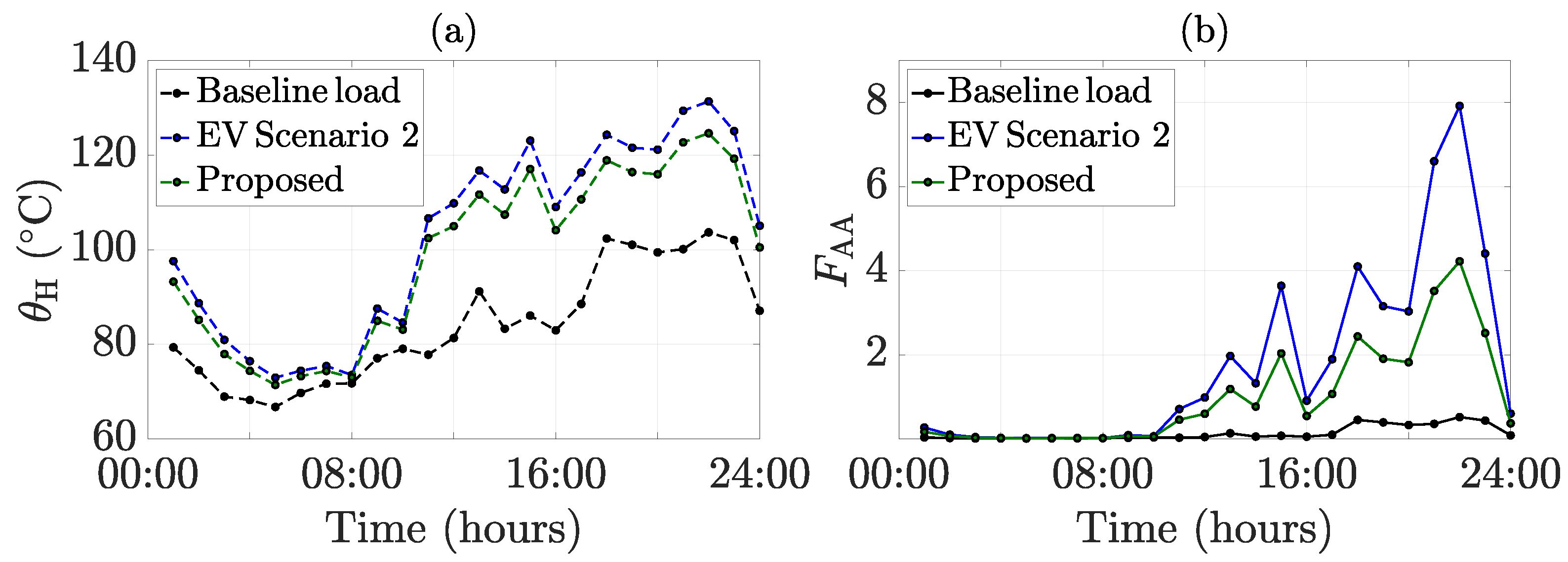
Figure 11.
Transformer life indices in scenario 2, (a) hottest-spot temperature, ; (b) accelerated aging factor, .
Figure 11.
Transformer life indices in scenario 2, (a) hottest-spot temperature, ; (b) accelerated aging factor, .
Figure 12.
Scenario 3: EV charging at Level 2, (a) number of EVs present; (b) transformer apparent power in kVA; (c) Q supplied by an online EV at Level 2 in kVAr; (d) transformer reactive power in kVAr.
Figure 12.
Scenario 3: EV charging at Level 2, (a) number of EVs present; (b) transformer apparent power in kVA; (c) Q supplied by an online EV at Level 2 in kVAr; (d) transformer reactive power in kVAr.
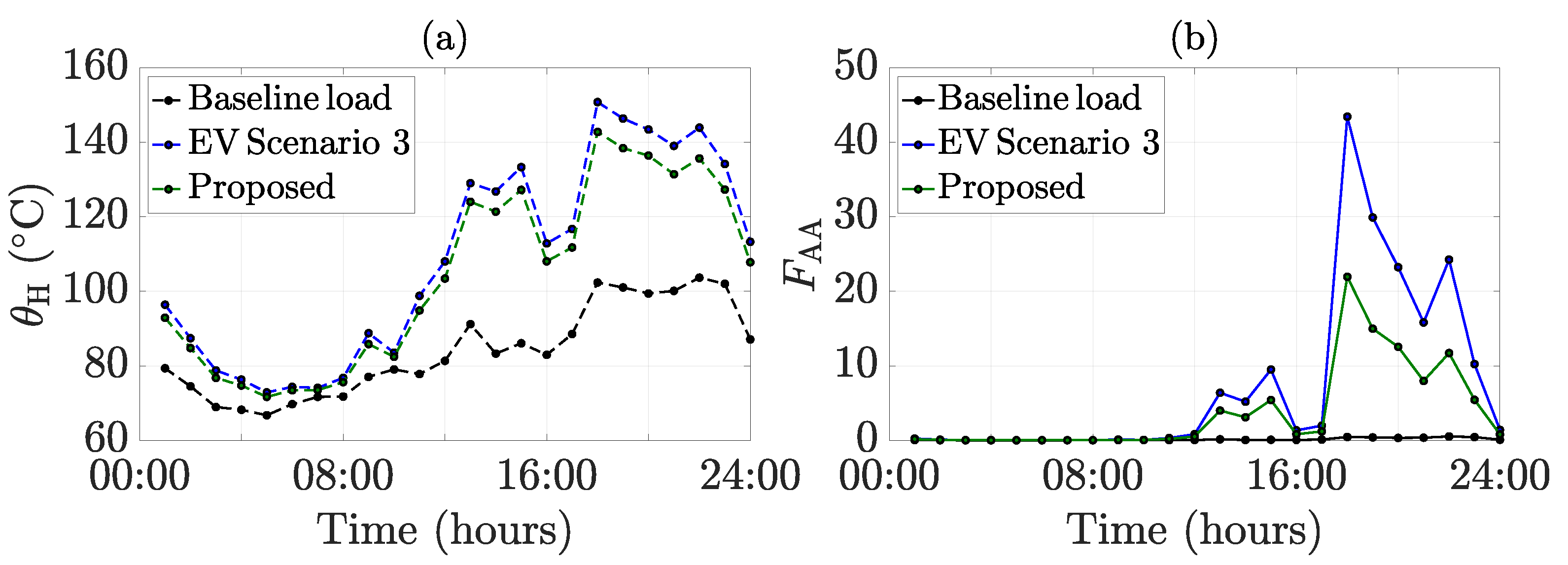
Figure 13.
Transformer life indices in scenario 3, (a) hottest-spot temperature, ; (b) accelerated aging factor, .
Figure 13.
Transformer life indices in scenario 3, (a) hottest-spot temperature, ; (b) accelerated aging factor, .
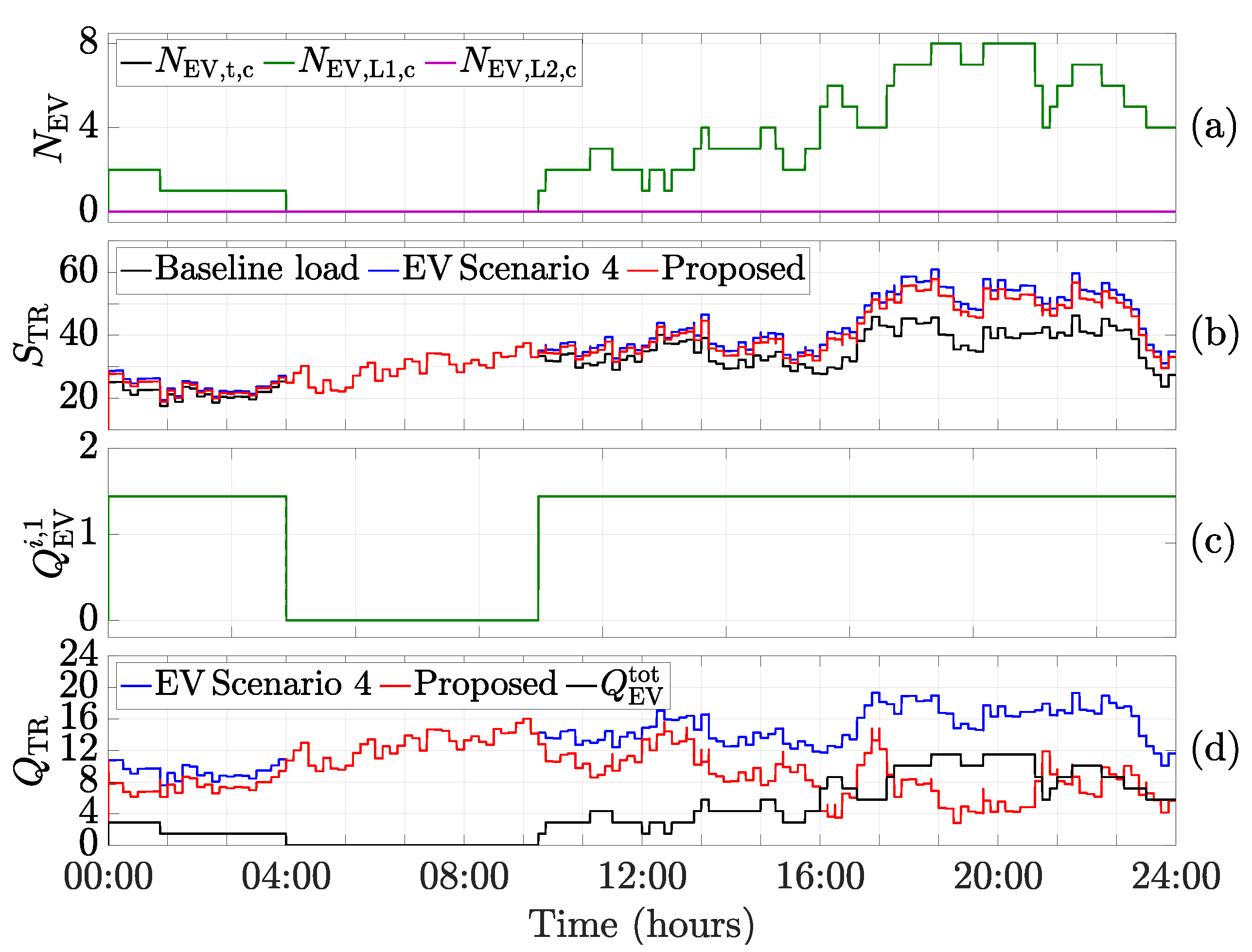
Figure 14.
Scenario 4: EV charging overlaps with peak load, (a) number of EVs present; (b) transformer apparent power in kVA; (c) Q supplied by an online EV at Level 1 in kVAr; (d) transformer reactive power in kVAr.
Figure 14.
Scenario 4: EV charging overlaps with peak load, (a) number of EVs present; (b) transformer apparent power in kVA; (c) Q supplied by an online EV at Level 1 in kVAr; (d) transformer reactive power in kVAr.
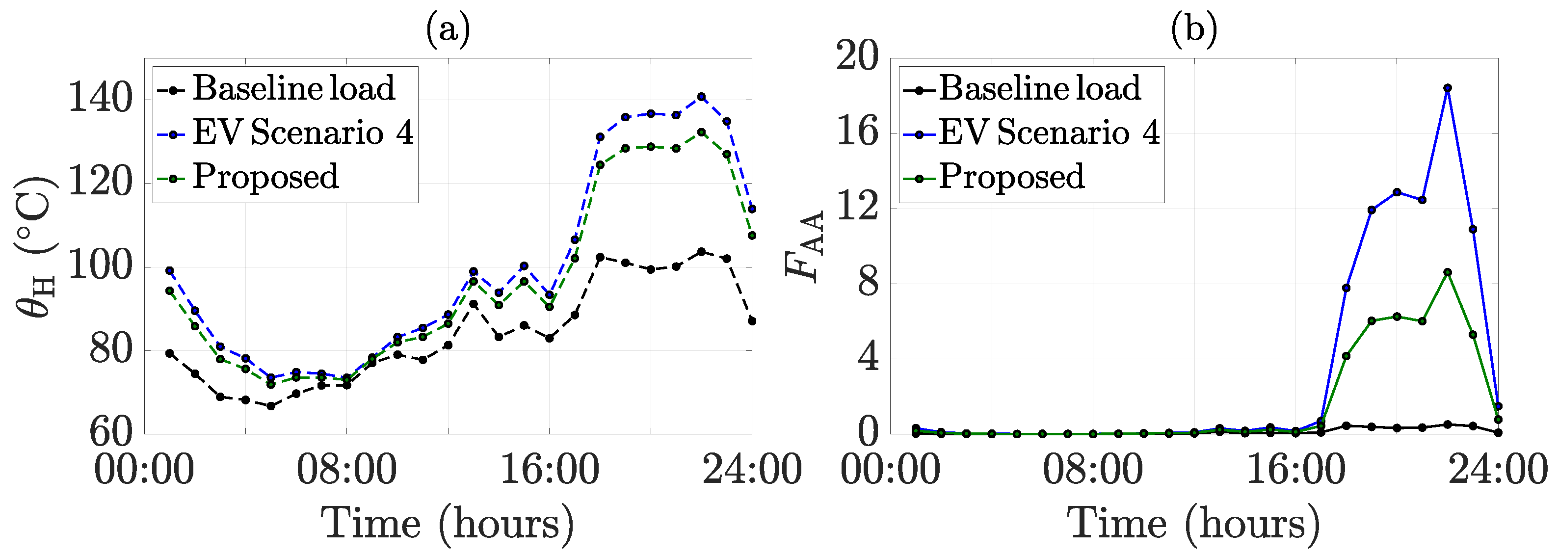
Figure 15.
Transformer life indices in scenario 4, (a) hottest-spot temperature, ; (b) accelerated aging factor, .
Figure 15.
Transformer life indices in scenario 4, (a) hottest-spot temperature, ; (b) accelerated aging factor, .
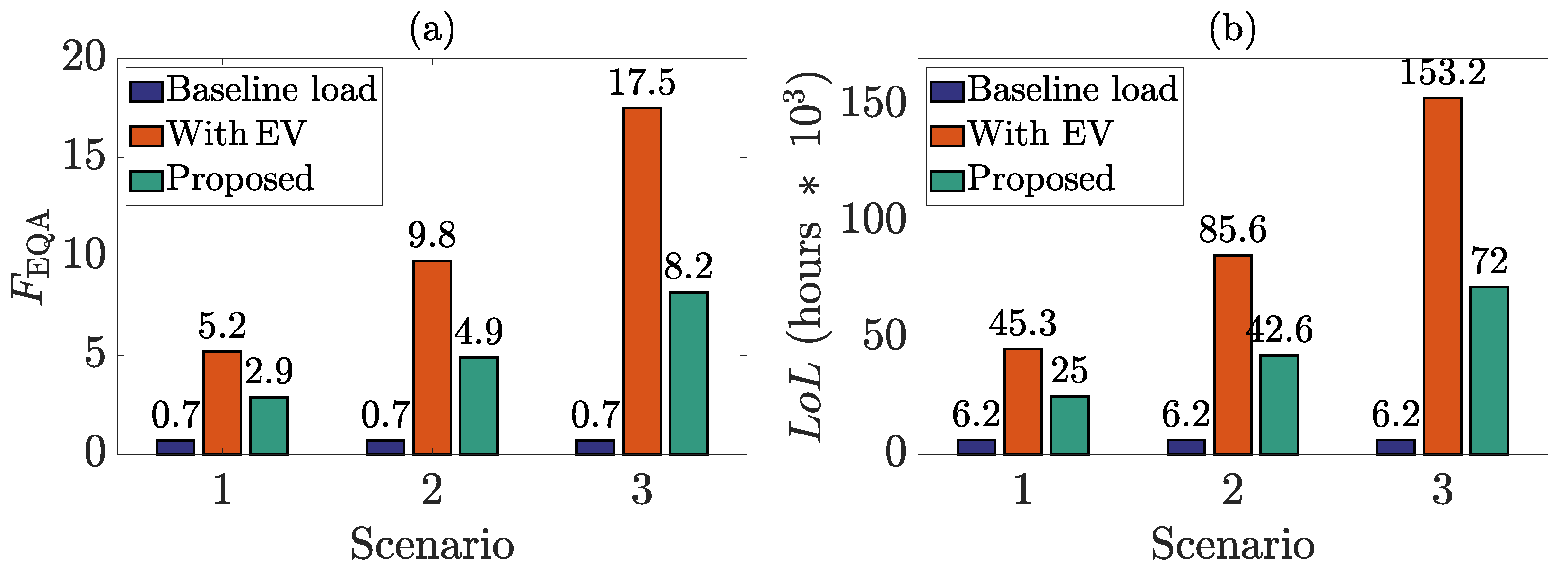
Figure 16.
Transformer’s annual (a) equivalent aging factor, ; and (b) loss of life, .
Figure 16.
Transformer’s annual (a) equivalent aging factor, ; and (b) loss of life, .
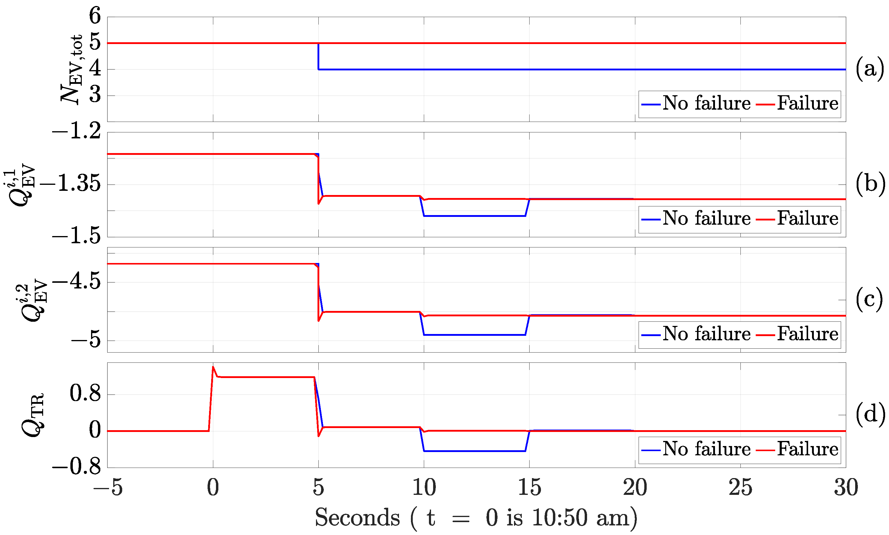
Figure 17.
System response without and with communication failure case 1, (a) number of EVs present; (b) Q supplied by an online EV at Level 1 in kVAr; (c) Q supplied by an online EV at Level 2 in kVAr; (d) transformer reactive power in kVAr.
Figure 17.
System response without and with communication failure case 1, (a) number of EVs present; (b) Q supplied by an online EV at Level 1 in kVAr; (c) Q supplied by an online EV at Level 2 in kVAr; (d) transformer reactive power in kVAr.
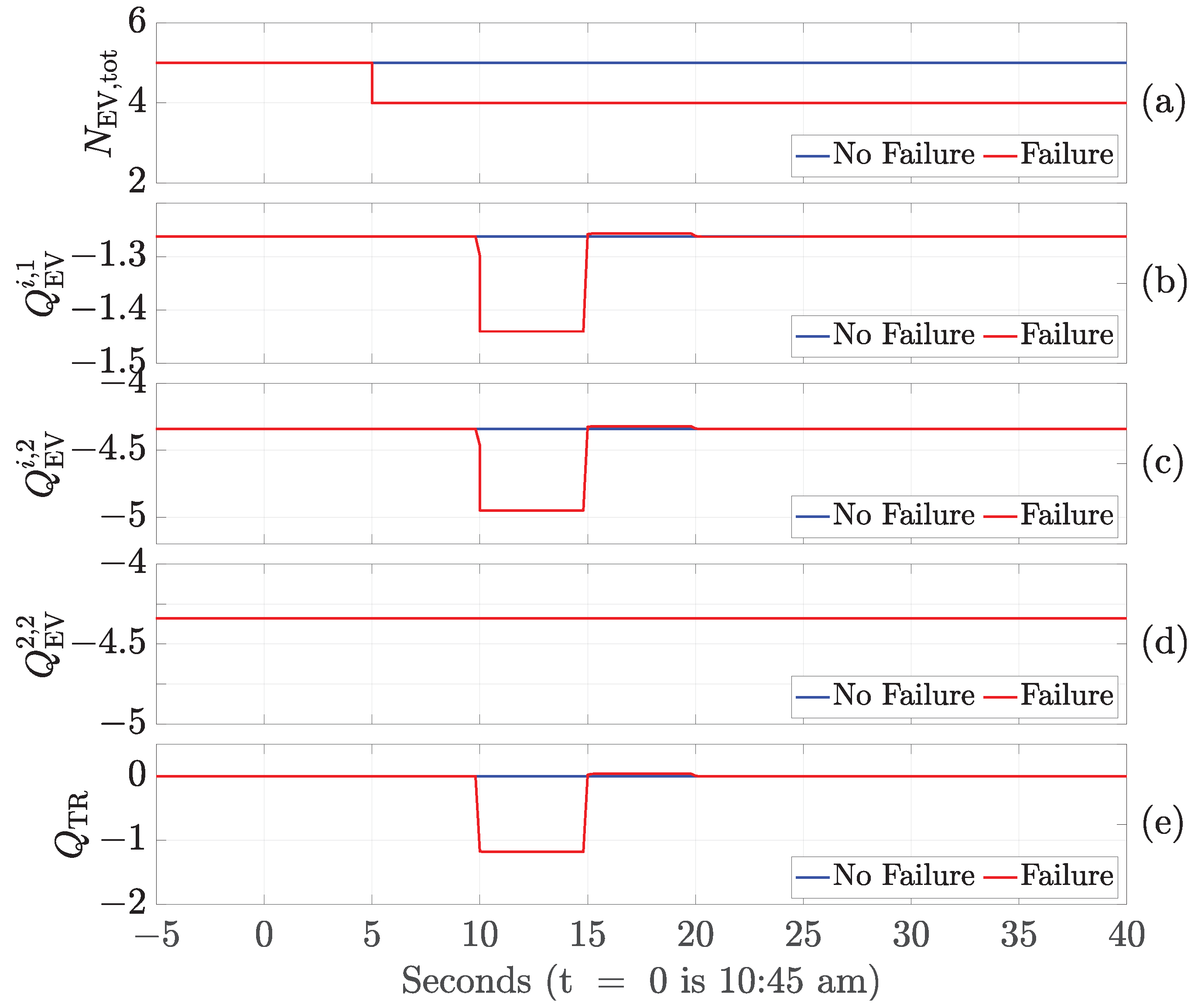
Figure 18.
System response without and with communication failure case 2, (a) number of EVs present; (b) Q supplied by an online EV at Level 1 in kVAr; (c) Q supplied by an online EV at Level 2 in kVAr; (d) Q supplied by EV-2 at Level 2 in kVAr; (e) transformer reactive power in kVAr.
Figure 18.
System response without and with communication failure case 2, (a) number of EVs present; (b) Q supplied by an online EV at Level 1 in kVAr; (c) Q supplied by an online EV at Level 2 in kVAr; (d) Q supplied by EV-2 at Level 2 in kVAr; (e) transformer reactive power in kVAr.
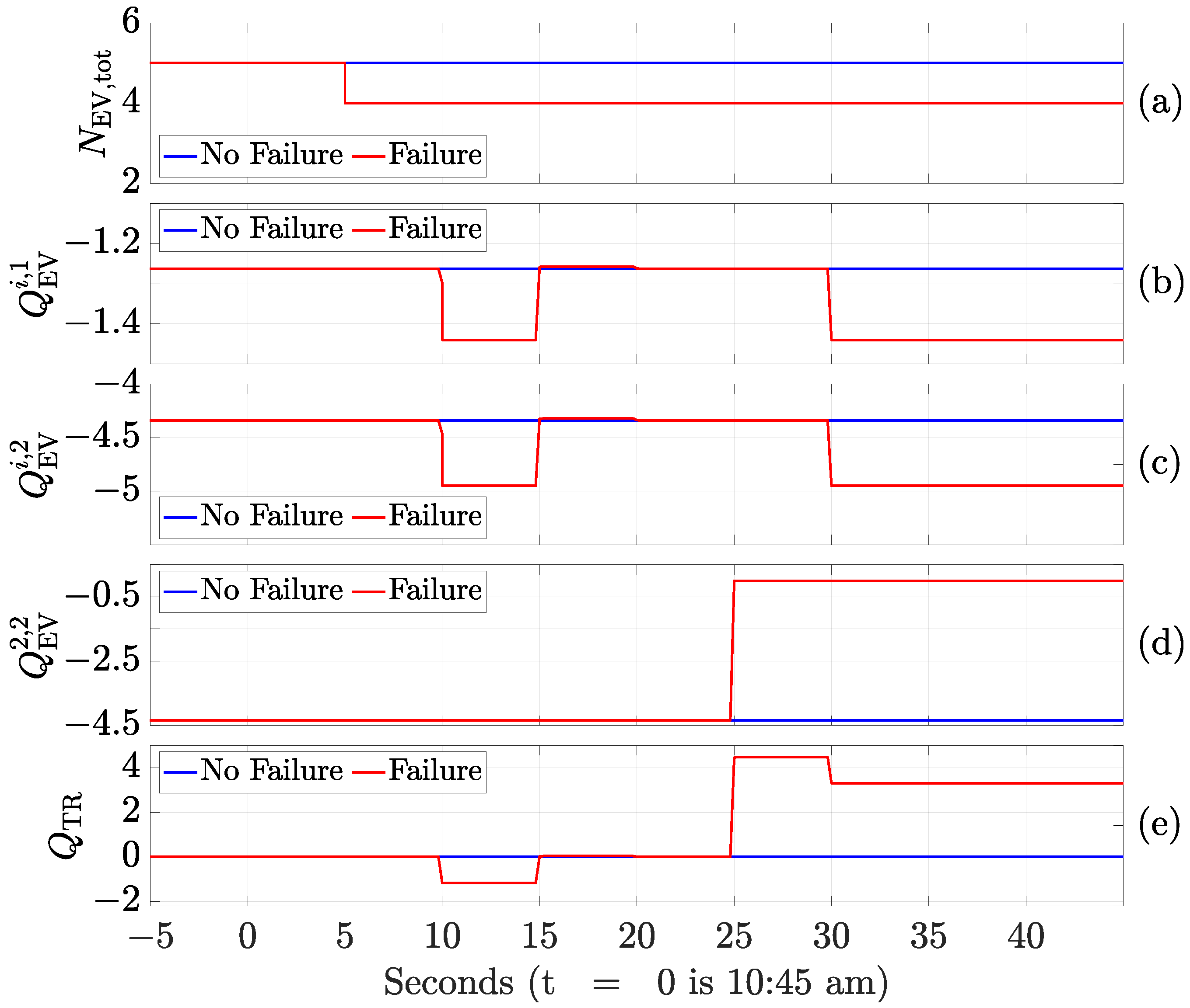
Figure 19.
System response without and with communication failure case 3, (a) number of EVs present; (b) Q supplied by an online EV at Level 1 in kVAr; (c) Q supplied by an online EV at Level 2 in kVAr; (d) Q supplied by EV-2 at Level 2 in kVAr; (e) transformer reactive power in kVAr.
Figure 19.
System response without and with communication failure case 3, (a) number of EVs present; (b) Q supplied by an online EV at Level 1 in kVAr; (c) Q supplied by an online EV at Level 2 in kVAr; (d) Q supplied by EV-2 at Level 2 in kVAr; (e) transformer reactive power in kVAr.
Table 1.
Transformer’s and without EV and with EV charging.
Table 1.
Transformer’s and without EV and with EV charging.
| Parameter | Baseline | Scenario 1 | Scenario 2 | Scenario 3 | Scenario 4 |
|---|
| 0.137 | 1.35 | 1.91 | 9.12 | 2.99 |
| 3.29 | 32.45 | 45.78 | 218.84 | 71.69 |
Table 2.
and in scenario 1.
Table 2.
and in scenario 1.
| System | | |
|---|
| Baseline load | 0.137 | 3.29 |
| EV Scenario 1 | 1.35 | 32.45 |
| Proposed method | 0.757 | 18.18 |
Table 3.
Root mean square deviation in voltages in scenario 1 with and without the proposed method.
Table 3.
Root mean square deviation in voltages in scenario 1 with and without the proposed method.
| Phase/Line | | | | | | |
|---|
| Bus No. | w/o Controller | with Controller | w/o Controller | with Controller | w/o Controller | with Controller |
|---|
| Bus 1 | 2.15 | 1.16 | 0.44 | 0.29 | 1.75 | 0.9 |
| Bus 2 | 1.98 | 1.06 | 0.38 | 0.27 | 1.65 | 0.8 |
| Bus 3 | 2.18 | 1.19 | 0.44 | 0.29 | 1.77 | 0.92 |
| Bus 4 | 2.05 | 1.1 | 0.41 | 0.28 | 1.69 | 0.84 |
| Bus 5 | 0.44 | 0.29 | 2.12 | 1.14 | 1.72 | 0.88 |
| Bus 6 | 0.45 | 0.29 | 2.15 | 1.16 | 1.74 | 0.9 |
| Bus 7 | 0.44 | 0.29 | 2.13 | 1.14 | 1.73 | 0.88 |
| Bus 8 | 0.48 | 0.3 | 2.24 | 1.22 | 1.8 | 0.94 |
| Bus 9 | 2.86 | 1.64 | 0.72 | 0.38 | 2.19 | 1.31 |
| Bus 10 | 2.87 | 1.64 | 0.72 | 0.38 | 2.19 | 1.31 |
| Bus 11 | 2.82 | 1.61 | 0.7 | 0.37 | 2.16 | 1.28 |
| Bus 12 | 0.58 | 0.34 | 2.53 | 1.41 | 1.99 | 1.11 |
| Bus 13 | 0.64 | 0.36 | 2.7 | 1.52 | 2.1 | 1.21 |
| Bus 14 | 0.28 | 0.09 | 0.34 | 0.09 | 0.6 | 0.16 |
| Bus 15 | 2.72 | 1.54 | 0.66 | 0.36 | 2.1 | 1.23 |
| Bus 16 | 0.57 | 0.33 | 2.49 | 1.38 | 1.96 | 1.09 |
| Bus 17 | 0.29 | 0.09 | 0.3 | 0.08 | 0.58 | 0.16 |
| Bus 18 | 0.29 | 0.09 | 0.3 | 0.08 | 0.58 | 0.16 |
| Bus 19 | 0.29 | 0.09 | 0.3 | 0.08 | 0.58 | 0.16 |
| Bus 20 | 0.57 | 0.33 | 2.49 | 1.38 | 1.96 | 1.09 |
Table 4.
and in scenario 2.
Table 4.
and in scenario 2.
| System | | |
|---|
| Baseline load | 0.137 | 3.29 |
| EV Scenario 2 | 1.91 | 45.79 |
| Proposed method | 1.08 | 25.92 |
Table 5.
Root mean square deviation in voltages in scenario 2 with and without the proposed method.
Table 5.
Root mean square deviation in voltages in scenario 2 with and without the proposed method.
| Phase/Line | | | | | | |
|---|
| Bus No. | w/o Controller | with Controller | w/o Controller | with Controller | w/o Controller | with Controller |
|---|
| Bus 1 | 1.6 | 0.88 | 0.74 | 0.35 | 1.84 | 0.94 |
| Bus 2 | 1.5 | 0.83 | 0.86 | 0.46 | 1.97 | 1.06 |
| Bus 3 | 1.41 | 0.75 | 0.8 | 0.38 | 1.76 | 0.86 |
| Bus 4 | 1.57 | 0.86 | 0.76 | 0.36 | 1.81 | 0.92 |
| Bus 5 | 1.5 | 0.83 | 1.04 | 0.58 | 2.4 | 1.33 |
| Bus 6 | 1.35 | 0.76 | 1.19 | 0.69 | 2.46 | 1.39 |
| Bus 7 | 1.42 | 0.83 | 1.25 | 0.74 | 2.59 | 1.53 |
| Bus 8 | 1.28 | 0.7 | 1.12 | 0.62 | 2.31 | 1.26 |
| Bus 9 | 1.74 | 0.99 | 1.01 | 0.56 | 2.07 | 1.17 |
| Bus 10 | 1.91 | 1.1 | 0.97 | 0.52 | 2.11 | 1.21 |
| Bus 11 | 1.77 | 1.01 | 0.97 | 0.54 | 2.1 | 1.21 |
| Bus 12 | 1.16 | 0.65 | 1.71 | 1.01 | 2.59 | 1.52 |
| Bus 13 | 1.19 | 0.66 | 1.49 | 0.86 | 2.48 | 1.41 |
| Bus 14 | 0.47 | 0.11 | 0.44 | 0.13 | 0.91 | 0.23 |
| Bus 15 | 1.75 | 0.99 | 0.94 | 0.51 | 2.04 | 1.14 |
| Bus 16 | 1.19 | 0.66 | 1.49 | 0.86 | 2.48 | 1.41 |
| Bus 17 | 0.39 | 0.09 | 0.34 | 0.11 | 0.73 | 0.2 |
| Bus 18 | 0.39 | 0.09 | 0.34 | 0.11 | 0.73 | 0.2 |
| Bus 19 | 0.39 | 0.09 | 0.34 | 0.11 | 0.73 | 0.2 |
| Bus 20 | 1.19 | 0.66 | 1.49 | 0.86 | 2.48 | 1.41 |
Table 6.
and in scenario 3.
Table 6.
and in scenario 3.
| System | | |
|---|
| Baseline load | 0.137 | 3.29 |
| EV Scenario 3 | 9.12 | 218.84 |
| Proposed method | 4.74 | 113.71 |
Table 7.
Root mean square deviation in voltages in scenario 3 with and without the proposed method.
Table 7.
Root mean square deviation in voltages in scenario 3 with and without the proposed method.
| Phase/Line | | | | | | |
|---|
| Bus No. | w/o Controller | with Controller | w/o Controller | with Controller | w/o Controller | with Controller |
|---|
| Bus 1 | 1.28 | 0.7 | 1.28 | 0.7 | 2.55 | 1.4 |
| Bus 2 | 1.32 | 0.75 | 1.32 | 0.75 | 2.65 | 1.5 |
| Bus 3 | 1.19 | 0.63 | 1.19 | 0.63 | 2.38 | 1.25 |
| Bus 4 | 1.21 | 0.65 | 1.21 | 0.65 | 2.42 | 1.29 |
| Bus 5 | 1.54 | 0.91 | 1.54 | 0.91 | 3.08 | 1.83 |
| Bus 6 | 1.52 | 0.89 | 1.52 | 0.89 | 3.04 | 1.77 |
| Bus 7 | 1.55 | 0.93 | 1.55 | 0.93 | 3.1 | 1.86 |
| Bus 8 | 1.44 | 0.83 | 1.44 | 0.83 | 2.89 | 1.66 |
| Bus 9 | 1.56 | 0.98 | 1.56 | 0.98 | 3.12 | 1.96 |
| Bus 10 | 1.62 | 1.03 | 1.62 | 1.03 | 3.24 | 2.07 |
| Bus 11 | 1.51 | 0.93 | 1.51 | 0.93 | 3.02 | 1.86 |
| Bus 12 | 1.93 | 1.29 | 1.93 | 1.29 | 3.86 | 2.57 |
| Bus 13 | 1.9 | 1.27 | 1.9 | 1.27 | 3.81 | 2.53 |
| Bus 14 | 0.62 | 0.17 | 0.62 | 0.17 | 1.23 | 0.33 |
| Bus 15 | 1.51 | 0.93 | 1.51 | 0.93 | 3.02 | 1.85 |
| Bus 16 | 1.81 | 1.18 | 1.81 | 1.18 | 3.63 | 2.36 |
| Bus 17 | 0.48 | 0.11 | 0.48 | 0.11 | 0.97 | 0.22 |
| Bus 18 | 0.48 | 0.11 | 0.48 | 0.11 | 0.97 | 0.22 |
| Bus 19 | 0.48 | 0.11 | 0.48 | 0.11 | 0.97 | 0.22 |
| Bus 20 | 1.81 | 1.18 | 1.81 | 1.18 | 3.63 | 2.36 |
Table 8.
and in scenario 4.
Table 8.
and in scenario 4.
| System | | |
|---|
| Baseline load | 0.137 | 3.29 |
| EV Scenario 4 | 2.99 | 71.69 |
| Proposed method | 1.49 | 35.83 |
Table 9.
Root mean square deviation in voltages in scenario 4 with and without the proposed method.
Table 9.
Root mean square deviation in voltages in scenario 4 with and without the proposed method.
| Phase/Line | | | | | | |
|---|
| Bus No. | w/o Controller | with Controller | w/o Controller | with Controller | w/o Controller | with Controller |
| Bus 1 | 2.2 | 1.14 | 0.42 | 0.3 | 1.81 | 0.87 |
| Bus 2 | 2.36 | 1.25 | 0.47 | 0.32 | 1.92 | 0.96 |
| Bus 3 | 2.19 | 1.14 | 0.41 | 0.3 | 1.81 | 0.87 |
| Bus4 | 2.19 | 1.14 | 0.41 | 0.3 | 1.81 | 0.87 |
| Bus 5 | 0.25 | 0.23 | 1.59 | 0.78 | 1.42 | 0.57 |
| Bus 6 | 0.25 | 0.23 | 1.59 | 0.78 | 1.42 | 0.57 |
| Bus 7 | 0.26 | 0.23 | 1.6 | 0.78 | 1.43 | 0.57 |
| Bus 8 | 0.3 | 0.24 | 1.75 | 0.88 | 1.52 | 0.66 |
| Bus 9 | 4.02 | 2.31 | 1.08 | 0.52 | 2.97 | 1.89 |
| Bus 10 | 3.93 | 2.24 | 1.04 | 0.51 | 2.91 | 1.83 |
| Bus 11 | 3.96 | 2.27 | 1.06 | 0.51 | 2.93 | 1.85 |
| Bus 12 | 0.67 | 0.36 | 2.82 | 1.58 | 2.2 | 1.27 |
| Bus 13 | 0.66 | 0.36 | 2.8 | 1.56 | 2.18 | 1.25 |
| Bus 14 | 0.24 | 0.11 | 0.57 | 0.12 | 0.79 | 0.09 |
| Bus 15 | 3.72 | 2.12 | 0.97 | 0.48 | 2.78 | 1.72 |
| Bus 16 | 0.58 | 0.34 | 2.57 | 1.41 | 2.04 | 1.12 |
| Bus 17 | 0.32 | 0.09 | 0.31 | 0.09 | 0.63 | 0.17 |
| Bus 18 | 0.32 | 0.09 | 0.31 | 0.09 | 0.63 | 0.17 |
| Bus 19 | 0.32 | 0.09 | 0.31 | 0.09 | 0.63 | 0.17 |
| Bus 20 | 0.58 | 0.34 | 2.57 | 1.41 | 2.04 | 1.12 |
Table 10.
Annual and in scenario 5 (40 % EV penetration).
Table 10.
Annual and in scenario 5 (40 % EV penetration).
| System | | (×1000 h) |
|---|
| Baseline load | 0.71 | 6.18 |
| EV Scenario 5 | 2.33 | 20.45 |
| Proposed method | 1.6 | 14 |


