Abstract
The increase in heterogeneous data in the building energy domain creates a difficult challenge for data integration. Schema matching, which maps the raw data from the building energy domain to a generic data model, is the necessary step in data integration and provides a unique representation. Only a small amount of labeled data for schema matching exists and it is time-consuming and labor-intensive to manually label data. This paper applies semantic-similarity methods to the automatic schema-mapping process by combining knowledge from natural language processing, which reduces the manual effort in heterogeneous data integration. The active-learning method is applied to solve the lack-of-labeled-data problem in schema matching. The results of the schema matching with building-energy-domain data show the pre-trained language model provides a massive improvement in the accuracy of schema matching and the active-learning method greatly reduces the amount of labeled data required.
1. Introduction
There are millions of buildings (residential, institutional, industrial buildings, etc.) around the world and they form a major part of the human energy footprint. Improving the energy efficiency of buildings helps reduce operational costs and curb carbon emissions [1]. To achieve this goal, coordination and cooperation between all companies in the building life cycle, from conceptualisation to refurbishment, is essential. Many building energy-efficiency solutions have been developed, tested and deployed [2]. With the rapid development and widespread application of advanced technologies such as computer technology, Internet of Things (IoT) technology, cloud-computing technology and sensing technology, the building energy sector is set to see comprehensive innovation and restructuring [3].
Smart buildings have emerged from this development. Smart buildings rely on new technologies such as IoT, big data, cloud computing and artificial intelligence in all the life stages of the building. In the last decade, the integration of intelligence (e.g., microcontrollers and microcomputers), sensors and networks (i.e., IoT connectivity) has become increasingly common in all types of buildings [4]. With the dramatic growth in building-energy-domain data over the past few years, individual devices and functional units generate thousands of terabytes of data per year, as these systems record operating parameters at second or minute intervals [5]. Building-related systems must handle millions of terabytes of data, and the next generation of building management systems will handle vast amounts of data. The data generated by these systems is complex and heterogeneous. This data, therefore, requires complex data processing before it can be used in a meaningful way, and the mapping of this metadata onto a semantic-information model requires domain expertise and is time-consuming.
Despite a number of architectures and underlying technological implementations of big-data solutions for buildings’ energy management [6], there is a lack of standardisation of the data model representing the meaning of the data [7]. This is referred to as a lack of semantic interoperability. Semantic interoperability is defined as the ability to use the information already exchanged between two or more systems or components. A lack of semantic interoperability is currently a significant problem [8] that hinders the streamlined integration of interdependent software applications and the development of applications that can be reused across buildings. To be of full value, digitised information and systems must be interoperable [9].
The main goal of this paper is to map raw data from the building energy domain into a generic data model, which is called schema matching. Schema matching [10] is a technique for identifying semantically related objects, i.e., finding the semantic correspondence between elements of two schemas, which is the structure behind the data organization [11]. Schema matching has usually been performed manually, which has significant limitations. Therefore, defining such mappings is a complex and time-consuming task. Additionally, only a small amount of labeled data for schema matching exists, especially in the building energy domain. Moreover, it may not be feasible during the coordination and cooperation between companies in the whole building life cycle. Therefore, to reduce manual effort and automate the schema-matching process, considerable research efforts have been made and techniques have been proposed: structure-based techniques, instance-based techniques and linguistic-based techniques [12].
As shown in Figure 1, the generic data model consists of multiple entities (also known as a class). Furthermore, each entity consists of multiple attributes, which are mainly in the form of a word or phrase. The raw dataset consists of three parts, the name of the dataset, attributes and instances. Each attribute in raw datasets is also in the form of a word or phrase which represents the descriptive information of the instances. The dataset’s name and attributes in the raw datasets and the entity’s name and attributes in the generic data model contain rich linguistic information to calculate semantic similarity. Therefore, the linguistic-based technique is very suitable to be applied to the schema matching in this paper. To automate schema matching, currently, the linguistic-based techniques are mainly implemented based on WordNet [13] or word-embedding techniques, such as Word2Vec [14]. However, with the development of the field of natural language processing (NLP), such as the BERT pre-training model in 2018 [15], which has successfully achieved state-of-the-art accuracy on 11 common NLP tasks, and other models based on BERT such as the Sentence-BERT model [16], etc., the field of schema matching has not been updated with these new techniques. Especially in the field of building energy, the level of digitalisation is relatively low. The technologies related to schema matching are even more outdated in this field. For example, Building Information Modelling (BIM) uses manual mapping or basic linguistic-based techniques to generate mapping candidates such as cosine similarity and Jaccard coefficients [17,18,19].
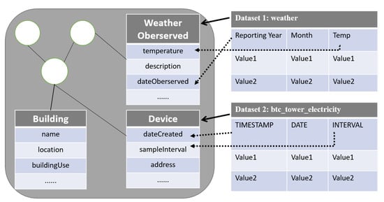
Figure 1.
Data model and raw data structure.
The schema-matching process uses two-step processes consisting of a dataset-level matching-process step followed by an attribute-level matching-process step. The dataset-level process is used to find the matching between datasets and entities in the generic data model, while the second process is used to obtain the final matching relationships between attributes in the raw datasets and attributes in the entities. In both processes, we use various semantic-similarity methods at different levels to perform experimental comparisons. These methods are divided into three main parts, string-based, knowledge-based and corpus-based, which include some classical similarity methods and new developments in the field of NLP. In addition, another approach based on active learning has been proposed and allows the selective aggregation of a number of similarity methods. This approach is also analysed in comparison with the previous methods. More specifically, the paper provides the following contributions:
- Proposes an overview of existing semantic-similarity approaches and applies a pre-trained language model for the schema-matching task;
- Introduces the active-learning method to solve the lack of labeled data in the building energy domain;
- Provides the evaluation of the existing semantic-similarity approach and pre-trained language model with datasets from the building energy domain in terms of accuracy.
The rest of this paper is structured as follows. Section 2 focuses on a literature review of schema matching, semantic-similarity calculation methods and active learning. Section 3 describes the implementation of the whole methodology in detail. Section 4 focuses on the performance of the developed method in the schema-matching process. Finally, Section 5 provides a summary of the work and an outlook for the future.
2. Literature Review
In this section, the existing approaches for schema mapping and the available methods to calculate semantic similarity are presented.
2.1. Schema Matching
Schema matching is a technique for finding semantic correspondence between elements of two schemas. In order to reduce the manual effort involved in schema matching, a number of solutions have been developed to automatically determine schema correspondences. Many linguistic-based similarity calculation methods have also been applied to schema matching, which is performed by calculating the semantic-similarity values of elements between the original data and the generic data model.
Erhard Rahm and Philip A. Bernstein [12] present a taxonomy covering a number of existing approaches, which they describe in some detail. They distinguish between schema-level and instance-level, element-level and structure-level, and language-based and constraint-based matchers. Based on their classification, they review some previous matchmaking implementations and, thus, indicate which part of the solution space they cover. Their taxonomy, alongside a review of past work, are helpful when selecting approaches to schema matching and developing new matching algorithms.
Giunchiglia and Yatskevich [20] propose an element-level semantic-matching approach by WordNet. The matchers use WordNet as a source of background knowledge and obtain semantic conceptual relationships from the database. The experimental results derived by the element-level matchers reflect as good a matching quality as that achieved by the matching systems of the Ontology Alignment Evaluation Initiative (OAEI 2006). The main limitation is this method based on WordNet, which contains only a limited amount of vocabulary for the building energy domain.
To solve the limitation of WordNet, Raul Castro Fernandez et al. [14] propose SEMPROP, which finds links based on syntactic and semantic similarities. SEMPROP is commanded by a semantic matcher which uses word embeddings to find semantically related objects. They also introduce coherent groups, a technique for combining word embeddings which works better than other state-of-the-art combination methods. However, this method ignores the different-granularities problem in schema matching.
Ayman Alseraf et al. [21] perform schema matching by collecting different types of content metadata and schema metadata about the dataset. They first propose a pre-filtering approach based on different granularities, in which they use data-analysis techniques to collect metadata. Their approach collects metadata at two different levels: the dataset and the attribute level. The proximity between the datasets is then calculated based on their metadata, their relationships are found based on the overall proximity and then similar pairs of datasets are obtained. Next, they introduce a supervised mining method to improve the effectiveness of this task to detect similar datasets that were used for pattern matching. They then conduct a number of experiments to demonstrate the success of their approach in effectively detecting similar datasets used for pattern matching. This work focuses more on general dataset matching. The performance of this method in the building energy domain data was not tested. Additionally, the pre-trained language model is not used to capture the semantic similarity between the datasets.
Benjamin Hättasch et al. [22] present a novel end-to-end schema-matching method based on a pre-trained language model. The main idea is to use a two-step approach consisting of a table-matching step and an attribute-matching step. With these two steps, they use embeddings at different levels, representing either whole tables or individual attributes. Their results show that this method is able to determine correspondences in a stable way. However, the lack-of-labeled-data problem was not considered in this work.
2.2. Semantic Similarity
Semantic similarity is used to identify concepts that share a common ’feature’ [23]. Semantic-similarity matching is essentially a measure of similarity between text data. The purpose is to capture the strength of semantic interactions between semantic elements (e.g., words, concepts) according to their meaning. It has many application scenarios, such as QA, automated customer service, search engines, semantic understanding, and automated marking, etc. To address this problem, various semantic-similarity methods have been proposed over the years. From traditional NLP techniques, such as string-based approaches, to the latest research work in the field of artificial intelligence, they are categorised into string-based methods [24], knowledge-based methods and corpus-based methods according to their underlying principles [25], which are summarised in Table 1.
2.2.1. String-Based-Method
In mathematics and computer science, a string metric (also known as a string similarity metric or string distance function) is a metric which measures the distance between two text strings for approximate string matching or comparison and in fuzzy string searching. A requirement for a string metric (e.g., in contrast to string matching) is the fulfillment of the triangle inequality. For example, the strings “Sam” and “Samuel” can be considered to be close [26]. A string metric provides a number indicating an algorithm-specific indication of distance.

Table 1.
Semantic-similarity methods.
Table 1.
Semantic-similarity methods.
| Types | Methods | Reference | Features |
|---|---|---|---|
| String-based | Edit distance | [27] | Based on features of glyphs, without semantics. |
| Jaccard | [28] | Similarities and differences between finite sample sets, without semantics. | |
| Knowledge-based | Wordnet | [29] | Structured words ontology, but too few words. |
| Wikipedia | [30] | A rich and updated corpus, but require networking and time-consuming. | |
| Corpus-based | Word2vec | [31] | Fast and generalized considering the context, but cannot solve polysemy. |
| Glove | [32] | Fast and generalized considering the context and global corpus, but cannot solve polysemy. | |
| Fasttext | [33] | Fast and represents rare words and out-of-lexicon words by n-gramm. | |
| BERT | [15] | Effectively extracts contextual information, but unsuitable for semantic-similarity search. | |
| Sentence-bert | [16] | Fast and over 100 languages. |
Edit distance: This method [27] is a quantitative measure of the degree of difference between two strings. Suppose a string a and a string b. The measure is to calculate how many operations are needed to change string a into string b. The operations include addition, deletion and replacement. Edit distance has applications in natural language processing, where automatic spelling correction can determine a candidate correction for a misspelled word by selecting words from the dictionary which have a low distance from the word.
Jaccard [28] index is a classical measure of set similarity with many practical applications in information retrieval, data mining, and machine learning, etc. [34]. The Jaccard distance, which measures the dissimilarity between sample sets, complements the Jaccard coefficient and is obtained by subtracting the Jaccard coefficient from 1 or, alternatively, by dividing the size of the union by the difference between the sizes of the union and the intersection of the two sets [35].
2.2.2. Knowledge-Based Method
In many applications dealing with textual data, such as natural language processing, knowledge acquisition and information retrieval, the estimation of semantic similarity between words is of great importance. Semantic-similarity measures make use of knowledge sources as a basis for estimation. The knowledge-based semantic-similarity approach calculates the semantic similarity between two terms based on information obtained from one or more underlying knowledge sources (e.g., ontology/lexical databases, thesauri, and dictionaries, etc.). The underlying knowledge base provides a structured representation of terms or concepts connected by semantic relations for these methods, further providing a semantic measure that is free of ambiguity, as the actual meaning of the terms is taken into account.
Wordnet [29] is characterized by a wide coverage of the English lexical–semantic network by organizing lexical information according to word meaning rather than word form. Nouns, verbs, adjectives and adverbs are each organized into a network of synonyms, each synonym set represents a basic semantic concept and these sets are also connected by various relations; a polysemantic word will appear in each of its meaning synonym sets. A synonymy set can be seen as a semantic relationship between word forms with a central role. Given a synonymy set, the Wordnet network can be traversed to find synonymy sets of related meanings. Each synonym set has one or more superordinate word paths connected to a root superordinate word. Two synonym sets connected to the same root may have some superordinates in common. If two synonym sets share a particular superlative, i.e., are at the lower level of the superlative hierarchy, they must be closely related. Therefore, we can perform the semantic-similarity calculation between words based on Wordnet, an ontology library.
In general, WordNet is a well-structured knowledge base, which includes not only general dictionary functions but, additionally, word-classification information. Therefore, based on Wordnet, similarity calculation methods are provided [36], such as the calculation of the shortest path between two words. The shortest distance between two words is obtained by calculating the relative position of each word in Wordnet and its closest common ancestor, and this distance is used to calculate the magnitude of similarity between them. However, its disadvantages cannot be ignored. It has only a limited number of words, so domain-specific words cannot be recognized, and, secondly, it cannot reflect the meaning of words in context.
Wikipedia is a large-scale knowledge resource built by Internet users who contribute freely and collaborate together in a way that creates a very practical ontology repository. In addition, it is completely open; the basic unit of information in Wikipedia is an article. Each article describes a single concept, and each concept has a separate article. Since each article focuses on a single issue and discusses that issue in detail, each Wikipedia article describes a complete entity.
Since articles contain, for example, titles, tables of contents, categories, text summaries, sections, citations, and hyperlinks, these can be considered as features of the concept. Therefore, it is natural to think of using Wikipedia’s conceptual features to measure the similarity between words. Since the titles of Wikipedia articles are concise phrases, similar to the terms in traditional thesauri, we can also think of the title as the name of the concept. To calculate the similarity value between two concepts, we can select some features to represent the concept. For example, the four parts of the Wikipedia concept—synonyms, glosses, anchors, and categories—can be considered as features representing the Wikipedia concept.
Jiang et al. [30] propose a feature-based approach which relies entirely on Wikipedia, which provides a very large domain-independent encyclopedic repository and semantic network for computing the semantic similarity of concepts with broader coverage than the usual ontology. To implement feature-based similarity assessment using Wikipedia, first, they present a formal representation of Wikipedia concepts. Then, a framework for feature similarity based on the formal representation of Wikipedia concepts is given. Finally, they investigate several feature-based semantic-similarity measures that emerge from instances of this framework and evaluate them. In general, several of their proposed methods have good human relevance and constitute some effective methods for determining similarities between Wikipedia concepts.
Knowledge-based systems are highly dependent on the underlying resources, resulting in the need for frequent updates, which require time and significant computational resources. While powerful ontologies such as WordNet exist in English, similar resources are not available in other languages, which necessitates the creation of robust, structured knowledge bases to enable knowledge-based approaches in different languages as well as in different domains.
2.2.3. Corpus-Based Method
Natural language is a complex system for expressing the thoughts of the human brain. In this system, words are the basic units of meaning. The technique of mapping words to real vectors is known as word embedding. Word embeddings use the distributional hypothesis to construct vectors and rely on information retrieved from large corpora; thus, word embeddings are part of a corpus-based approach to semantic similarity. The distribution hypothesis presents a view in which words with the same meaning are grouped together in a text. This view examines the meanings of words and their distribution throughout the text and then compares them with the distribution of words with similar or related meanings, the basic principle of which is simply summarised as ’similar words occur together frequently’. In recent years, word embeddings have gradually become essential knowledge for natural language processing. Word embeddings take a vector representation of words and provide a vector of meaning for them, preserving the underlying linguistic relationships between words. Methods for word embedding include artificial neural nets [31], dimensionality reduction in word co-occurrence matrices, and explicit representation of the context in which words occur.
Word2vec takes a text corpus as input, first constructs a vocabulary from the training text data, and then learns a vector representation of the words. It maps each word to a vector of fixed length, which better expresses the similarity and contrast between words. Tomas Mikolov et al. [31] propose two new model structures, the CBOW and Skip-gram models, for computing continuous vector representations of words from very large datasets. The quality of these representations was measured in word and syntactic-similarity tasks, and the results were compared with previous best-presentation techniques based on different types of neural networks which can be trained to produce high-quality word vectors using very simple model architectures. They show that it is possible to compute very accurate high-dimensional word vectors from much larger datasets at much lower computational costs.
In summary, Word2vec can be trained to obtain its weight matrix through two different structures, and this weight matrix is the word-vector dictionary we want to obtain in the end. In this, each word has its corresponding word vector to represent. Therefore, when calculating the similarity between different words, the similarity can be calculated using their word vectors. In the Google Word2vec model used in this matcher, the word-vector table is mainly composed of some phrases and words, in which the words are basically lowercase words and the upper case words are not recognized; therefore, the words to be calculated need to be preprocessed when using this model. Moreover, this method can be regarded as a word-vector dictionary based on corpus training; thus, for some special abbreviations or words that are not in the word-vector dictionary, the word vector it represents cannot be queried, and it cannot be used for the calculation of lexical similarity. In addition, since the word-vector relationship is one-to-one, the problem cannot be solved for words with multiple meanings, such as “bank”.
Glove: Jeffrey Pennington et al. [32] constructed a new global log-linear regression model, which they call GloVe, for unsupervised lexical-representation learning which outperforms other models on lexical-analogy, lexical-similarity and named-entity-recognition tasks because the statistics of the global corpus are captured directly by the model. The model combines the strengths of two major families of models: the global matrix- decomposition method and the local context-window method. The model makes effective use of statistical information by training only the non-zero elements of the word–word co-occurrence matrix, rather than the entire sparse matrix or a single context window in a large corpus. The model produces a vector space with meaningful substructures. In addition, it outperforms the correlation model on similarity tasks and named-entity recognition.
Fasttext: In linguistics, morphology studies word formation and lexical relationships. However, Word2vec and GloVe do not explore the internal structure of words. The fastText [33] model proposes a subword insertion method, which assumes that a word consists of n characters, which is an n-gram. There are some advantages of using n-grams, which can generate better word vectors for rare words. For character-level n-grams, that is, the word appears very few times, but the characters that make up the word share parts with other words, so this can optimize the generated word vectors, and, in the case of lexical words, it is still possible to construct word vectors for words from character-level n-grams even if the words do not appear in the training corpus. In addition to this, the n-gram allows the model to learn partial information about the local word order.
Neither word2vec nor GloVe can provide word vectors for words that do not exist in the dictionary. Compared to them, fastText has the following advantages: first of all, it works better for word vectors generated from low-frequency words. This is because their n-grams can be shared with other words. Secondly, for words outside the training lexicon, their word vectors can still be constructed. We can superimpose their character-level n-gram vectors. Thus, when using it for lexical similarity computation, an important feature of fastText is its ability to generate word vectors for any word, even for words that do not occur, assembled words and some specialized domain abbreviations. This is mainly because fastText builds word vectors from substrings of characters contained in words, so this way of training the model allows fastText to generate word vectors for misspelled or concatenated words. In addition, fasttext is also faster than other methods, which makes it more suitable for computing on small data sets.
BERT [15] is the Bidirectional Encoder Representation from Transformers pre-trained model. The BERT model has achieved excellent results in various NLP tests; the network architecture of BERT uses the encoder-side structure of the multilayer transformer proposed in this work. Attention is all you need, and the overall framework of BERT consists of two phases: pre-train and fine tune. In contrast to Word2vec or GloVe, for example, “bank”, the same word has different meanings in different contexts. However, embedding such as Word2Vec will only provide the same word embedding for “bank” in these different contexts. Compared with Word2vec, it can also obtain word meanings according to the sentence context, thus avoiding ambiguity.
Sentence-BERT: Due to the excellent performance of the BERT model, many scholars later conducted much research based on BERT. Sentence-BERT is also based on the BERT model by extending its application.
Nils Reimers and Iryna Gurevych [16] proposed Sentence-BERT (SBERT), a modification of the BERT network using siamese and triplet networks, which is able to derive semantic sentence embeddings. This allows BERT to be used for certain new tasks. This framework can be used to compute sentence/text embeddings in over 100 languages. These embeddings can then be compared, for example, using cosine similarity to find sentences with similar meanings. This is useful for semantic text similarity, semantic searching or paraphrase mining. This model is trained on all available training data (over 1 billion training pairs) and is designed to be a general-purpose model. It is not only fast but maintains high quality.
3. Methodology
In Figure 2, the schema-matching approach and implementation process are described in detail. The large-scale pilot (LSP) raw datasets and the data model were the input for the schema-matching process. To calculate the semantic similarity between raw datasets and data model, the pairs set is generated through data processing. The pairs set is the attribute pairs between raw data and the data model. The calculated similarity is used to process dataset-level matching and generate the matching between dataset and the entity in the data model. The attribute-level matching takes the dataset-level matching as input and generates the final mapping table.
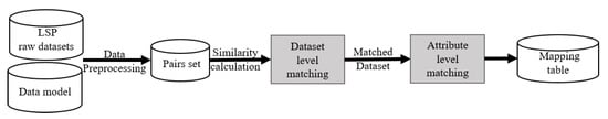
Figure 2.
Schema mapping process overview.
3.1. Data Preprocessing
The data preprocessing step, which can be used in a selective combination to automate the pre-processing of raw data, is necessary. As the data are mainly from the field of building energy domain, they have their own specificity in that the attribute contains special symbols (e.g., _, -, ( , ), &) and directly connects words together, such as ‘alternateName’, ‘floorHeight’ and ‘energySource’. In addition, similarity calculation methods have different applicability requirements for their input data, which is described in Section 2.2. Therefore, it is important to pre-process these metadata before the semantic-similarity matching calculation. The data preprocessing is summarised in three categories: symbol handling, phrase handling and word landing.
Symbol handling: Although most data attributes consist of only letters, words, and phrases, there may be special symbols interspersed. Therefore, before performing the semantic-similarity calculation, it is necessary to remove them according to the requirements of similarity-matching calculation methods, which were described in the previous section. For example, ‘Energy_Source’ is converted to ‘Energy Source’.
Phrase handling: Some words or phrases in the metadata may be misspelled, so it is necessary to correct the misspelling of the words. In addition, some metadata in the field of building energy have special features, for example, some words in the phrase are directly connected together, such as ‘alternateName’, ‘floorHeight’ and ‘energySource’ and so on. These linked phrases cannot be directly utilized in some lexical-similarity calculation methods because their semantics cannot be identified. Therefore, the lexical segmentation of such phrases is performed to automatically separate their words. For example, ‘energySource’, is corrected to ‘energy Source’.
Word handling: The word handling consists of three parts: word cases, tokenization and stemming. Word-case handling ensures uniformity of the words to be matched by coverting all the words to lower case; word tokenization splits a correctly spelled phrase into individual words, e.g., ‘energy Source’ is split into two words in the form of ‘energy’ and ‘source’. The stemming is performed on the split words, which will have different word forms, such as different tenses of verbs, singular or plural nouns, etc. Therefore, the root of words is found and used for further semantic-similarity calculation. These operations can be used in selective combinations to meet the requirements of different semantic-similarity calculation methods. For example, the Wiki-cons-based matcher is sensitive to word cases and the tenses of verbs.
3.2. Dataset Level
The dataset-level matching process produces the matching of pairs between datasets and entities. The goal is to find the matching entity for each dataset and to reduce the computation effort of semantic-similarity calculation.
Generation of pairs: A matrix of dataset-pairs matching similarity scores each other is generated as in Table 2, where the = {dataset 1, dataset 2, dataset 3, …}, = {entity 1, entity 2, entity 3, …}. The similarity score of each dataset pair is .
Table 2.
Datasets to entities pairs.
Algorithm: The matrix of the overall similarity scores of all dataset pairs can be calculated through the most efficient matcher. Each dataset is matched with possible related entities in the dataset-level matching process, which is a one-to-many matching process. Some datasets may not match any entity. In this regard, a threshold value is set to 0.1, and when the overall similarity between a pair of datasets is less than the threshold value, the similarity score of this pair will be set to zero. The dataset-level schema matching is summarised in Algorithm 1.
| Algorithm 1: Dataset level schema matching |
| Input: The set of datasets and the set of entities Output: matching result of and and similarity scores
|
3.3. Attribute Level
Generation of pairs: The matching process at the attribute level only focuses on an individual dataset. Each dataset is composed of multiple attributes, = {attr_1, attr_2, attr_3, …}. Each entity in the data model is also composed of multiple attributes, = {attr_1, attr_2, attr_3, …}. The attribute-pairs matrix is obtained as in Table 3, according to this data structure. The similarity value between each attribute pair is .
Table 3.
Attributes- pairs matrix.
Algorithm: the attribute-pairs matrix generated by one dataset and entity pair is computed based on different matchers, as shown in Table 4, to obtain a matrix of similarity values between attribute pairs.
Table 4.
Example 1: Attributes-pairs matrix with similarity scores calculated by one matcher.
Next, the attribute pairs are filtered based on the similarity scores in the matrix. The matching principle is that each matches at most one , but each can match multiple attributes in the same dataset at the same time. However, each can match multiple attributes of the same dataset at the same time. According to this matching principle, all attribute pairs are ranked according to their similarity scores, and filtered according to the highest similarity score. For that have already been selected, the attribute pairs containing will not be considered in the next matching step. When all pair combinations are selected, a matching table of attributes is obtained, as shown in Table 5.
Table 5.
Example 1: Attributes-pairs matching result.
In addition, in the process of calculating the similarity of the matched matrices, a threshold value can be set, which means that if the similarity score of an attribute pair is less than the threshold value of 0.3, the score will be 0, and it is directly determined as no match. Finally, the overall similarity between the respective dataset and entity is calculated using Equation (1) from the similarity scores of these attribute pairs, which is averaged here. n is the number of attributes in the dataset. The attribute-level schema matching is described in Algorithm 2.
| Algorithm 2: Attribute-level similarity calculation |
| Input: Attributes set of a dataset and the attributes set of an entity Output: Mapping result of attributes between and in form of , which contains scores and matching relationships of Attributes
|
3.4. Matching Process at the Combined Dataset and Attribute Level
The matching work at the attribute-level and dataset-level granularity are described above. The matching between attribute pairs is performed at the attribute level, and the matching between dataset pairs is performed at the dataset level. Therefore, the two are combined to build the whole dataset-matching computational model.
Algorithm 3 is divided into two parts: dataset-level and attribute-level matching processing. The dataset-level matching processing focuses on the similarity relationship between datasets and uses unsupervised matching. First, the similarity scores of dataset pairs formed by the datasets and entities are calculated by the most efficient matcher, which is presented and tested in Section 4. Then, the dataset pairs are initially selected by combining the top-k strategy to select potentially similar dataset pairs. The top-k strategy selects the k entities with the highest similarity score for one dataset. This is a relatively simple and rapid way of calculating semantic similarity at the dataset level. In the attribute-level matching processing, only these k entities are matched separately for detailed calculation. With this model, the overall computation can be effectively reduced, the computational efficiency can be improved, and the matching process can be accelerated.
| Algorithm 3: Matching process combined dataset and attribute level |
| Input: The set of datasets, the set of entities and different matchers Output: After two levels of matching, the final matching result in form of DataFrame based on different matchers
|
3.5. Active Learning
As shown in Table 1, each method has its advantages and disadvantages. In order to make better use of the features of different methods and to bring out the advantages of different matchers, we aggregated these methods.
The relevant aggregation methods are maximum, minimum and standard average. Maximum (minimum) means that the similarity scores between the terms are calculated using different matchers, and the maximum (minimum) is taken as the overall similarity value between the two terms. Standard average means that the similarity scores calculated by different matchers are averaged as the overall similarity score between the terms. However, in cases in which some methods have features that go well with the specifics of the problems and others do not, the averaging appears detrimental. Therefore, if different matchers can be assigned different weights, the characteristics of different matchers can be fully exploited. To achieve the assignment of the weights, the active-learning method is applied. Another reason for using active learning is that it reduces the amount of labeled data significantly. Especially for the building energy domain, only very limited labeled data is available for schema mapping.
Active learning is a method of machine learning which takes data from samples that are “hard” to classify. These data are then manually labeled and then trained with machine-learning models to gradually improve the effectiveness of the model. In general, we do not know how much labeled data is needed to obtain the expected results, so we want to obtain as many labeled samples as possible. However, in fact, the performance of the model does not increase wirelessly with the amount of labeled data, and there is a corresponding bottleneck in the performance of the model; therefore, we focus precisely on how to use as little labeled data as possible to reach this bottleneck.
Therefore, using active learning, we can actively select the most valuable samples for labeling and achieve the best performance of the model using as few high-quality samples as possible. According to the literature [37], active-learning models require only a small amount of labeled data to achieve higher performance compared to other models that require all training data for training. It is important to state that active learning is not guaranteed to improve the accuracy of classification models and is still mainly used to minimize the cost of labeling while ensuring that the model achieves the expected accuracy.
With active learning, the training and validation data required for the same machine-learning model are significantly reduced and achieve the same performance, as the candidate set extraction of the data to be labeled relies on the query function in active learning. The overall process of active learning is described in Figure 3. The first three steps are the same as in the schema-matching process, which obtains the input and calculates the attribute similarity. The attribute similarity is formed as a feature vector and used as input for the training process for active learning. The active learner is a machine-learning model, which is a classifier for schema matching. The active-learning model starts learning with a small number of initially labeled samples, selects one or a batch of the most useful samples by a certain query function, asks the oracle for labels, and then uses the new knowledge gained to train the classifier and perform the next round of queries. Active learning is a cyclical process performed until a certain stopping criterion is reached.
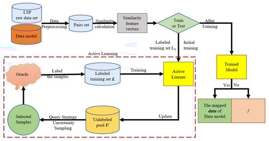
Figure 3.
Active-learning workflow.
3.5.1. Similarity Feature Vector
Attributes from the original datasets and attributes from the data model are combined to form a dataset consisting of vocabulary pairs through the pre-processing step described in Section 3.1. The similarity scores of these pre-processed pairs are calculated by matchers. Therefore, assume that the lexical similarity score between the vocabulary and the vocabulary is . In order to aggregate the matchers, we first compute the similarity of using different matchers. By treating the similarity score of each matcher as a feature, a pair of attributes can, thus, produce an n-dimensional similarity feature vector with Equation (2), where n is the number of matchers. By computing the entire dataset of vocabulary pairs, a dataset consisting of n-dimensional similarity feature vectors can be obtained, where the number of feature vectors is equal to the number of attribute pairs, and each feature vector represents the similarity relationship between two attributes.
3.5.2. Query Strategy
In general, labeling data is actually a tricky problem. The oracle needs to have relevant domain expertise, and, secondly, it is very costly and has a long lead time. Therefore, it is a meaningful task to train the model with a small amount of labeled data. In the field of active learning, the key is how to select the appropriate annotation candidates for manual annotation, and the method of selection is the so-called query strategy. Suppose the matching between the dataset attribute and entity attribute takes the value of 0 or 1, where 0 means two words do not match and 1 means they match each other. Therefore, this type of problem can be transformed into a problem of binary classification. Therefore, for any n-dimensional similarity feature vector, 0 or 1 is its corresponding manual annotation. The active-learning model used is “Pool-based Active Learning”. Initially, only the unlabeled data are available, and the query strategy needs to select data from the pool of unlabeled data and send it to an oracle for labeling. In the field of active learning, the key is how to select the appropriate annotation candidates for manual annotation, and the method of selection is the so-called query strategy.
The most commonly used query strategy is “uncertainty sampling”. The uncertainty-sampling query method extracts the indistinguishable sample data from the model; the algorithm only needs to query the most uncertain samples to oracle labeling. Usually, the model can quickly improve its performance by learning the labels of samples with high uncertainty. The key of the uncertainty-sampling method is how to describe the uncertainty of the sample or data. There are usually the following ways: least confident, margin sampling, and entropy methods. Compared to least confident and margin sample, the entropy approach considers all categories of the binary classification task. Therefore, the entropy method is selected as the query strategy.
3.5.3. Classifier
The classifier is a machine-learning model which consists of two parts: training and prediction. The similarity-feature-vector dataset computed by matchers is used as input. The data selected from the pool of unlabeled data by query strategy is labeled by oracle. The labeled data is then used to train the classifier. The two processes of querying the unlabeled data for manual labeling and training the model work alternately, and the performance of the benchmark classifier will gradually improve after several cycles. The process terminates when the preset conditions are satisfied. The preset conditions are generally information such as the amount of query data, i.e., the amount of manually labeled data, or the expected model accuracy. The classifier selected in this paper is a random forest model.
The random forest model is a supervised machine-learning algorithm. It is a classifier which contains multiple decision trees and its output is determined by the majority voting of the classes output by the individual trees. Training can be highly parallelized and can run efficiently on large data sets. Due to its accuracy, simplicity and flexibility, it has become one of the most commonly used algorithms. The fact that it can be used for classification and regression tasks, combined with its nonlinear nature, makes it highly adaptable to a variety of data and situations. In theory, a large number of unrelated decision trees will produce more accurate predictions than a single decision tree. This is because a large number of decision trees working in concert can protect each other from individual errors and over-fitting. In addition, because of the sampling of the decision-tree candidates to divide the attributes, the model can still be trained efficiently when the sample features are of high dimensionality. The final trained model has a high generalization capability.
After the training of the active-learning model, the model is used as a matcher in our schema-matching task. This is evaluated in the next section.
4. Results
In this chapter, based on the various matchers introduced in the previous chapter and combined with experimental data, experiments were set up to evaluate their performance in the schema-matching task. The device configuration used to conduct these experiments is the processor with an Intel(R) Core(TM) i5-8500 CPU @ 3.00 GHz, 8 GB of RAM and a 64-bit operating system. The details of these experiments are described in the following.
4.1. Setup
Dataset: the experimental datasets come from 11 different city administrations, network operators, suppliers, building management companies, and the building construction and renovation sectors. The data model was created based on the existing data model (e.g., FIWARE [38] and EPC4EU [39]). In the previous section, a brief description of the structure of the data model was given. A total of 28 entities are in the data model, they come from 12 different categories, and the number of attributes in all the entities is 755. The raw data to be matched are 25 datasets, of which there are 140 attributes.
Ground truth: to evaluate the computational results of the model, it is necessary to know the correct matching objects for the data to be matched. After manual annotation and classification, these 25 original datasets were assigned to the appropriate entity, and 140 of these attributes were assigned to the corresponding attribute in the corresponding entity. This was to find suitable matches for the dataset and attributes in the data model.
MRR, known as mean reciprocal rank, evaluates the top-k results. MRR is used to confirm that there is only one match and its correlation level is only relevant and irrelevant. It is very suitable for the determination of dataset-level matching processing in the model because each dataset has only one entity that is its correct match. Therefore, the ranking of the correct matching object among the k objects can be calculated for each dataset and its top-k entities. Equation (3) is shown in the following, where denotes the ranking position of the first relevant result, denotes the number of queries, and MRR denotes the average inverse ranking of the search system under the query set Q.
F1-score is a statistical measure of the accuracy of a binary classification model, which takes into account both the precision and recall of the classification model. Equation (4) of f1 scores can be considered as a harmonic average of the accuracy and recall of the model, with its maximum value being 1 and minimum value being 0.
In the evaluation process, there are four common cases: true positive (TP), false negative (FN), false positive (FP) and true negative (TN). The first true and false modify the later positive/negative, and the later positive and negative are the judgments of our methods. means that our method predicts positive, which is right, i.e., factually positive and predicted by our method as positive; means that our method predicts negative, which is wrong, i.e., factually positive but predicted by our method as negative. means that our method is predicted to be true, which is a wrong judgment, i.e., a situation which is not in fact true but is misjudged to be true by our method; means that our method predicted to be negative, which is a right judgment, i.e., a situation which is, in fact, negative and is predicted to be negative by our method.
Equation (5) is precision, which is the ratio of the number of facts that are positive and predicted to be positive as well as the number of results predicted to be positive, including those that are not correctly identified. Precision is also referred to as the positive predictive value.
Equation (6) is recall, which is the ratio of the number of samples in which the fact is positive and the judgment is also positive to the number of samples in which all facts are positive. The recall is also referred to as sensitivity in diagnostic binary classification.
4.2. ALmatcher
In addition to using different matchers for schema matching, we also propose active learning based on the aggregation of different machers, and then using the trained model to perform schema matching. “Active learning" (sometimes called “query learning” or “optimal experimental design” in the statistics literature) is a subfield of machine learning and, more generally, artificial intelligence [40]. In order to train the active-learning model, i.e., ALmatcher, the process is as follows.
4.2.1. Preparation of Training Data
Based on the actual dataset for this project, a total of 49,815 pairs could be generated, of which a total of 103 pairs were correctly matched, while there were 49,712 pairs that did not match. This is a typical problem for unbalanced categories, as the data is from a real-world sample. An unbalanced dataset is one in which the difference in number between the two categories of the dataset, the major and minor categories, reaches 100:1, 1000:1 or even 10,000:1 in a classification problem. Such a dataset will largely limit the accuracy of our classification models. When a standard learning algorithm encounters unbalanced data, the rules generalised to describe the smaller category are usually fewer and weaker than those describing the larger category. With this class of dataset, our goal becomes making the classification accuracy of the minor class as good as possible without seriously compromising the accuracy of the major class [41]. Therefore, we consider the use of a random-sampling-based approach, which is divided into random oversampling and random undersampling. The idea of random oversampling is to replicate a number of random-sample points from a minor class and add them to the original set to equalise the dataset. Random undersampling, on the other hand, removes a number of sample points at random from a major class to equalise the distribution of the dataset. Random undersampling may result in the loss of important information, while random oversampling risks overfitting. In order not to lose important information, random oversampling is used here to equalise the sample set.
After a relatively balanced sample set is then obtained, different matchers are used to generating similarity feature vectors as described in Section 3. Since nine matchers are used in this method, the whole data sample set consists of a nine-dimensional similarity feature vector. In order to train the active-learning model, the obtained sample set was divided into training and validation sets according to the ratio of 70% and 30%, where the training set was 69,598 and the validation set was 29,826. The following, Figure 4, shows the distributions of the similarity feature vectors of training samples and validation samples. They are represented by principal component analysis (PCA) with a dimensionality reduction process, where purple points represent mismatches with a label of ’0’ and yellow points represent matches with a label of ’1’. The training set is used to train the active-learning model, while the validation set is used to check its accuracy. The level of accuracy represents the evaluation parameter of the model’s ability to distinguish between the two categories.
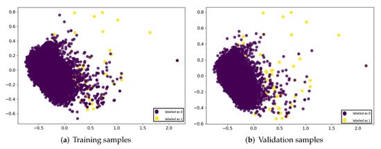
Figure 4.
Similarity feature vectors distribution.
4.2.2. Training and Validation
The initial basic model is obtained by first initialising the learner to be trained. Its machine-learning model is a random forest model. The validation set was used to test its accuracy. As shown in Figure 5a, below, it can be seen that the prediction accuracy of the untrained model on the validation set is 71.80%, where the green dot means that the predicted category of the classification is the same as the actual category of the label, i.e., the prediction is correct. The red dots indicate that the predicted results do not match the actual ones, i.e., the prediction is wrong.
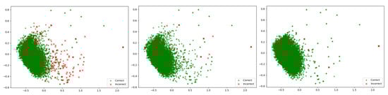
Figure 5.
Class prediction. (a) Untrained model: class predictions of validation samples (accuracy: 71.80%), (b) trained model: class predictions of validation samples (accuracy: 90.47%), (c) trained model: class predictions of rest (accuracy: 90.08%).
The query strategy is entropy sampling, whereby the data with the highest uncertainty are selected from the pool of data in the training set and manually annotated. The process is repeated until the model fulfills the stop criteria. The stop criteria is usually the number of queries, time or target performance. Here, is used as the stopping condition, and represents the accuracy of the training model in the validation set. From the experimental results, as shown in Figure 5b, it can be seen that using active learning only requires 2485 annotated data, i.e., 2485 queries to achieve of 90.47%, which constitutes a significant reduction in sample annotation cost and improvement in the performance of the classifier. Even if the trained model is used to predict the remaining unqueried data, as shown in Figure 5c, the accuracy can still reach 90.08%.
The results are analysed and the active-learning approach efficiently selects unclassified samples with high classification contribution for the annotation and training of the model. In practical application scenarios, active learning can significantly reduce the cost of labeling by selecting the most difficult samples for the relevant domain experts through some selection strategies. The trained model, i.e., ALmatcher, can be used in the schema-matching process to perform matching calculations and compare with other matchers.
4.3. Schema Matching
As shown in Algorithm 3, schema matching is divided into two processes: dataset-level matching processing and attribute-level matching process. The dataset-level matching process performs the initial filtering of pairs of datasets, using a top-k strategy, where for each dataset to be matched, k similar entities are first filtered out. The attribute-level matching process is a more detailed calculation. For the k candidate entities, the matching calculation is performed by comparing a number of different matchers.
4.3.1. Dataset-Level Matching Process
In this process, there are 700 pairs of dataset pairs to be computed formed by 25 datasets and 28 entities, of which there are approximately 100,000 attribute pairs. As this is an initial screening, the computational time of the method and its performance needs to be considered in this process. In addition, the choice of k-worthiness is debatable. Therefore, a number of experiments were set up here for evaluation.
Experiment 1: in preliminary screening, time consumption is a relatively important parameter. Therefore, in this process of preliminary screening, experiments based on different similarity calculation methods can be performed to obtain the time consumption of different similarity methods, as shown in Table 6.
Table 6.
The time consumption of different similarity calculation matchers in dataset-level matching process.
The shortest of these is Sentence-BERT, which takes only 1.41 min. The construction of BERT makes it unsuitable for unsupervised tasks such as semantic-similarity search and clustering. The longest is the Wikipedia-based approach, which takes over 2300 min. The reason is that it is based on the features of Wikipedia entries for similarity computation, so the network is heavily influenced by the query, and, in addition to this, the amount of information contained in the feature points of the entries can lead to long computation times. The knowledge-based approach is also wordnetpathsim, which takes about 16 min in the schema-matching process, and is calculated using synonym set features from the existing knowledge graph Wordnet, and, therefore, takes a little longer. In addition to sBERT and BERT, Word2vec, GloVe and fastText are also used for word vector-based computation, as they are based on the generated word vector model and, therefore, take less time. The remaining string-based methods, edit distance and Jaccard, also take less time to compute matches as they only take into account the morphological features of the words.
Experiment 2: the dataset-level matching processing focuses on the matching process between pairs of datasets, where a top-k strategy is chosen to select the k potential matching entities of the target dataset, and, therefore, in addition to the computation time, the performance of the matching results of the different matchers is the focus of reference. In this case, we aim to reduce the computational effort of the next attribute-level matching process and retain more information through the top-k initial filtering. Therefore, the choice of k is also crucial, as too large a number of items can retain more information, but it does not reduce the computational effort of the initial screening, while too small a number of key items will be lost. Therefore, here we choose k = 3 and k = 1 for comparison. As shown in Table 7, the MRR evaluation function and the F1-score evaluation function are used to evaluate the matching results of the dataset pairs, respectively. For the MRR evaluation function, where represents the sum of the reciprocal of the ranking of the correct match among the k entities that have a potential relationship with the target dataset that lie among these k entities. MRR is the quotient of the sum of its rank inverse and its total number of query objects, i.e., datasets. For the f1 score, it is an equilibrium function of PRECISION and RECALL. If the k entities matched by each dataset are considered as a whole, a match is considered successful in the dataset-level matching process if there is a correct match for its corresponding dataset in the k entities. Thus, where precision represents the ratio of the number of successful matches in the prediction to the number of all predictions that are true, recall represents the number of successful matches in the prediction to the number of correct matches in reality.
Table 7.
Evaluation of dataset-level matching process.
It can be seen that when k = 3, the performance is significantly improved compared to k = 1. In addition, in general, the former involved 75 pairs of dataset pairs in the next step and the latter 25 pairs. Compared to the original 700 pairs, although both are reduced by an order of magnitude in computation and serve as an initial filter, the former also retains relatively more critical information. Therefore, in the subsequent attribute-level matching process, experiments were conducted based on a k value of 3.
Based on the experimental results of the top-k strategy and the computation time consumption, the matcher based on sentence BERT is a better choice in the dataset-level matching-process, not only is the computation time consumption short, but also its performance is excellent. Therefore, in the next attribute-level matching process, we can compare the results of schema matching based on different matchers in detail, based on the top-three results of sentence BERT.
4.3.2. Attribute-Level Matching Process
In order to obtain an intuitive picture of the matching performance of the attribute-level matching process, the benchmark for the evaluation process is, therefore, based on the results of the dataset level, i.e., the evaluation of a total of 123 attributes for the 22 datasets that were initially matched correctly at the dataset level. The evaluation function is used to judge the performance of the different matchers in schema matching.
Experiment 3 The f1-score evaluation function is used to evaluate the results for the attribute-level matching process. As shown in Table 8, below, represents the number of correct attributes matched by different matchers in the matching process; represents the number of attributes that are in fact correct in the standard answer, where the number of correct answers is not the same as the number of attributes involved in the matching process; 108 for correct and 123 for involved. represents the number of attributes predicted to be positive by different matchers in the matching process.
Table 8.
Evaluation of attribute-level matching process.
These values are used to calculate the f1 score for different matchers. The data in the building energy domain in this project has its own peculiarities, not only in terms of special abbreviations and non-English words but also in terms of special matches, such as ‘power’ which may be matched with ‘value’. This experiment analyzes the evaluation results of different matchers in the application of schema matching. In particular, this schema matching process uses an unsupervised matching approach, based only on the similarity values between their words for schema matching.
The edit distance and Jaccard are calculated only from the lexical glyph features. Therefore, the results are better only for cases where the lexical features in the dataset are similar, e.g., using edit distance ‘DATE’ may be more similar to ‘NAME’ than to ‘DateCreated’. Jaccard is calculated based only on the number of letters in common between the two words. When two words are synonymous or have fewer letters in common, Jaccard will not match correctly. The wordnet calculation is based on the set of synonyms in the dictionary. It is difficult to apply this method when the whole word is queried directly as a whole in the process. Therefore, here, individual words from their phrases are used for the query, and, finally, their mean value is used to represent the similarity between the two phrases. The Wiki-cons are calculated mainly based on the features of Wikipedia entries on the web. Experiment 1 shows that this approach is very time-consuming, so the calculation is performed directly using the phrase to query the entries, rather than querying individual words in the phrase; otherwise, the time spent would increase exponentially. However, due to the specific nature of the data, many words are not actually available on Wikipedia and, therefore, as can be seen from the evaluation results, do not perform well, even worse than the wordnet-based approach for the word-embedding-based approach to similarity matching calculations. Among the two approaches Word2vec and GloVe, GloVe gives slightly better results than Word2vec because it takes into account the global nature, but the overall results are not very different. FastText, because it uses the n-gramm approach, will have some better results for specific words in the dataset, and this is reflected in the evaluation results. Applying the basic BERT to schema matching, the results are found to be not good, and the analysis of the literature [22] and matching results shows that since this method adopts unsupervised matching based on similarity values, the BERT approach is very high for all similarity values between different words and lacks significant differentiation. The sentence-BERT approach, when calculating the similarity between different words, shows that the distinction between similar words and dissimilar words is very obvious, and it is also very good for the calculation of word groups. However, it can only be used for matching between the same language, not across languages, and, secondly, it is not able to match correctly for specific matching relationships. ALmatcher is based on this experimental dataset using active learning, which has the highest f1 score. It combines the previous matchers and trains a model with a query strategy using only 2485 annotations with uncertainty. The trained model was applied to the actual schema matching and good results were achieved. Although the model is only annotated with a very small amount of data, it shows that this is a good direction, which does reduce the cost of manual annotation and has a good performance.
4.3.3. Matching Process at the Combined Dataset and Attribute Level
Experiment 4: the overall matching results are analysed through the above two processes. Data integration is where each dataset in the original dataset is matched to an entity in the generic data model, where their attributes are also matched to each other. As seen above, there are 25 raw data datasets and 140 attributes. The results are shown in Table 9, below. Comparing the results of all the matchers, we can see that the best performance is achieved by ALmatcher and sentence-BERT, which have 19 and 16 correct matches, respectively, and 76 and 59 correct matches for attributes during data harmonization. The rest of the matches were relatively poor, but it can be seen that some matchers had a lower number of correct matches for the datasets, but the number of correct matches for the attributes they contained was higher than those with a higher number of matches for the other datasets. In addition, the overall performance of the word-embedding-based matchers is relatively good.
Table 9.
Result of the overall schema matching.
This section focuses on the specific performance of different matchers, including method aggregation, in schema matching through various experimental comparisons. From these experimental comparisons, the strengths and weaknesses of the different matchers for building energy-domain applications are evaluated.
5. Conclusions
This paper successfully implemented the existing semantic-similarity calculation method for the schema-matching task in the building energy domain by combining knowledge from the natural language processing domain. Based on the semantic similarity between their attributes, schema matching was performed to integrate the raw data from the building energy domain into a common standard data model. Three types of lexical-similarity calculation methods, string-based methods (edit distance and Jaccard), knowledge-based methods (wordnet and Wikipedia-based methods) and corpus-based methods (word2vec, GloVe, fastText, BERT and sentence BERT) were implemented. After comparing the experimental results, the pre-trained language-model-based matcher performed better than the other matchers in terms of accuracy. The sentence-BERT performed especially well in schema matching, both in terms of computational time and accuracy. Through active learning, different similarity approaches were aggregated based on the lexical similarity vectors, which were obtained by the different approaches. Based on the experiment result, the active-learning method provides better performance than other matches with a small amount of labeled data in the building energy domain. Therefore, it is recommended to use sentence-BERT, if there is no labeled data available. If it is possible to have a domain expert label a small amount of data, the active-learning matcher is better than all other unsupervised matchers.
In the future, the problem of unbalanced data sets remains; random sampling was chosen to solve this problem in this paper, but other approaches and text can be chosen. The current work focus on the attribute level and dataset level. The value of a dataset, which belongs to the instance level, was not utilized. The integration of instance-level schema mapping utilizes all the information from the dataset and has the potential to improve the overall performance. Furthermore, the similarity feature vector utilised by the active-learning training model is computed from each of the previously mentioned matchers. However, in future specific applications, for example, certain features in the similarity feature vector can be used or replaced selectively depending on time-consumption requirements. It is not limited to the matchers used in this paper but can be replaced using other similarity calculation methods depending on actual needs.
Author Contributions
Conceptualization, Z.P.; methodology, Z.P.; software, G.P.; validation, G.P. and Z.P.; formal analysis, Z.P.; investigation, Z.P.; resources, Z.P. and A.M.; data curation; writing—original draft preparation, Z.P. and G.P.; writing—review and editing, Z.P. and G.P.; visualization, G.P. and Z.P.; supervision, A.M.; project administration, A.M.; funding acquisition, A.M. All authors have read and agreed to the published version of the manuscript.
Funding
This research was funded by MATRYCS, which is a European project funded by the European Union’s Horizon 2020 research and innovation program under Grant Agreement No. 1010000158.
Institutional Review Board Statement
Not applicable.
Informed Consent Statement
Not applicable.
Data Availability Statement
Not applicable.
Acknowledgments
The authors would like to thank all the MATRYCS consortium partners.
Conflicts of Interest
The authors declare no conflict of interest.
References
- Lucon, O.; Urge-Vorsatz, D.; Ahmed, A.Z.; Akbari, H.; Bertoldi, P.; Cabeza, L.; Liphoto, E. Gadgil Chapter 9—Buildings. Clim. Chang. 2014. [Google Scholar]
- Balaji, B.; Bhattacharya, A.; Fierro, G.; Gao, J.; Gluck, J.; Hong, D.; Johansen, A.; Koh, J.; Ploennigs, J.; Agarwal, Y.; et al. Brick: Metadata schema for portable smart building applications. Appl. Energy 2018, 226, 1273–1292. [Google Scholar] [CrossRef]
- Makridakis, S. The forthcoming information revolution: Its impact on society and firms. Futures 1995, 27, 799–821. [Google Scholar] [CrossRef]
- Pritoni, M.; Weyandt, C.; Carter, D.; Elliott, J. Towards a Scalable Model for Smart Buildings. Lawrence Berkeley National Laboratory. 2021. Available online: https://escholarship.org/uc/item/5b7966hh (accessed on 19 November 2022).
- Benndorf, G.A.; Wystrcil, D.; Réhault, N. Energy performance optimization in buildings: A review on semantic interoperability, fault detection, and predictive control. Appl. Phys. Rev. 2018, 5, 041501. [Google Scholar] [CrossRef]
- Pau, M.; Kapsalis, P.; Pan, Z.; Korbakis, G.; Pellegrino, D.; Monti, A. MATRYCS—A Big Data Architecture for Advanced Services in the Building Domain. Energies 2022, 15, 2568. [Google Scholar] [CrossRef]
- Bergmann, H.; Mosiman, C.; Saha, A.; Haile, S.; Livingood, W.; Bushby, S.; Fierro, G.; Bender, J.; Poplawski, M.; Granderson, J.; et al. Semantic Interoperability to Enable Smart, Grid-Interactive Efficient Buildings; Lawrence Berkeley National Lab. (LBNL): Berkeley, CA, USA, 2020. [Google Scholar] [CrossRef]
- Pritoni, M.; Paine, D.; Fierro, G.; Mosiman, C.; Poplawski, M.; Saha, A.; Bender, J.; Granderson, J. Metadata schemas and ontologies for building energy applications: A critical review and use case analysis. Energies 2021, 14, 2024. [Google Scholar] [CrossRef]
- Greer, C.; Wollman, D.; Prochaska, D.; Boynton, P.; Mazer, J.; Nguyen, C.; FitzPatrick, G.; Nelson, T.; Koepke, G.; Hefner, A.; et al. NIST Framework and Roadmap for Smart Grid Interoperability Standards, Release 3.0, 2014. Available online: https://tsapps.nist.gov/publication/get_pdf.cfm?pub_id=916755 (accessed on 19 November 2022).
- Do, H.H.; Rahm, E. Chapter 53-COMA—A system for flexible combination of schema matching approaches. In Proceedings of the VLDB ’02: Proceedings of the 28th International Conference on Very Large Databases, Hong Kong, China, 20–23 August 2002; Bernstein, P.A., Ioannidis, Y.E., Ramakrishnan, R., Papadias, D., Eds.; Morgan Kaufmann: San Francisco, CA, USA, 2002; pp. 610–621. [Google Scholar] [CrossRef]
- Peukert, E.; Maßmann, S.; König, K. Comparing Similarity Combination Methods for Schema Matching. In Proceedings of the GI Jahrestagung, Leipzig, Germany, 27 September–1 October 2010. [Google Scholar]
- Rahm, E.; Bernstein, P. A Survey of Approaches to Automatic Schema Matching. VLDB J. 2001, 10, 334–350. [Google Scholar] [CrossRef]
- Chen, N.; He, J.; Yang, C.; Wang, C. A node semantic similarity schema-matching method for multi-version Web Coverage Service retrieval. Int. J. Geogr. Inf. Sci. 2012, 26, 1051–1072. [Google Scholar] [CrossRef]
- Fernandez, R.C.; Mansour, E.; Qahtan, A.A.; Elmagarmid, A.K.; Ilyas, I.F.; Madden, S.; Ouzzani, M.; Stonebraker, M.; Tang, N. Seeping Semantics: Linking Datasets Using Word Embeddings for Data Discovery. In Proceedings of the 34th IEEE International Conference on Data Engineering, ICDE 2018, Paris, France, 16–19 April 2018; Computer Society: Washington, DC, USA, 2018; pp. 989–1000. [Google Scholar] [CrossRef]
- Devlin, J.; Chang, M.W.; Lee, K.; Toutanova, K. BERT: Pre-training of Deep Bidirectional Transformers for Language Understanding. arXiv 2018, arXiv:1810.04805. [Google Scholar]
- Reimers, N.; Gurevych, I. Sentence-BERT: Sentence Embeddings using Siamese BERT-Networks. arXiv 2019, arXiv:1908.10084. [Google Scholar]
- Cheng, J.; Deng, Y.; Anumba, C. Mapping BIM schema and 3D GIS schema semi-automatically utilizing linguistic and text mining techniques. ITcon 2015, 20, 193–212. [Google Scholar]
- Mannino, A.; Dejaco, M.C.; Re Cecconi, F. Building Information Modelling and Internet of Things Integration for Facility Management—Literature Review and Future Needs. Appl. Sci. 2021, 11, 3062. [Google Scholar] [CrossRef]
- Charef, R.; Emmitt, S.; Alaka, H.; Foucha, F. Building Information Modelling adoption in the European Union: An overview. J. Build. Eng. 2019, 25, 100777. [Google Scholar] [CrossRef]
- Giunchiglia, F.; Yatskevich, M.; Shvaiko, P. Semantic Matching: Algorithms and Implementation. J. Data Semant. IX 2007, 9, 1–38. [Google Scholar] [CrossRef]
- Alserafi, A.; Abelló, A.; Romero, O.; Calders, T. Keeping the Data Lake in Form: Proximity Mining for Pre-Filtering Schema Matching. ACM Trans. Inf. Syst. 2020, 38, 1–30. [Google Scholar] [CrossRef]
- Hättasch, B.; Truong-Ngoc, M.; Schmidt, A.; Binnig, C. It’s AI Match: A Two-Step Approach for Schema Matching Using Embeddings. arXiv 2022, arXiv:2203.04366. [Google Scholar]
- Slimani, T. Description and evaluation of semantic similarity measures approaches. arXiv 2013, arXiv:1310.8059. [Google Scholar] [CrossRef]
- Caldarola, E.G.; Rinaldi, A.M. An approach to ontology integration for ontology reuse. In Proceedings of the 2016 IEEE 17th International Conference on Information Reuse and Integration (IRI), Pittsburgh, PA, USA, 28–30 July 2016; pp. 384–393. [Google Scholar]
- Chandrasekaran, D.; Mago, V. Evolution of semantic similarity—A survey. ACM Comput. Surv. (CSUR) 2021, 54, 1–37. [Google Scholar] [CrossRef]
- Lu, J.; Lin, C.; Wang, W.; Li, C.; Wang, H. String Similarity Measures and Joins with Synonyms. In Proceedings of the 2013 ACM SIGMOD International Conference on Management of Data, New York, NY, USA, 22–27 June 2013; Association for Computing Machinery: New York, NY, USA, 2013. SIGMOD ’13. pp. 373–384. [Google Scholar] [CrossRef]
- Levenshtein, V.I. Binary Codes Capable of Correcting Deletions, Insertions and Reversals. Sov. Phys. Dokl. 1966, 10, 707. [Google Scholar]
- Jaccard, P. The distribution of the flora in the alpine zone 1. New Phytol. 1912, 11, 37–50. [Google Scholar] [CrossRef]
- Miller, G.A. WordNet: A Lexical Database for English. Commun. ACM 1995, 38, 39–41. [Google Scholar] [CrossRef]
- Jiang, Y.; Zhang, X.; Tang, Y.; Nie, R. Feature-based approaches to semantic similarity assessment of concepts using Wikipedia. Inf. Process. Manag. 2015, 51, 215–234. [Google Scholar] [CrossRef]
- Mikolov, T.; Chen, K.; Corrado, G.; Dean, J. Efficient Estimation of Word Representations in Vector Space. arXiv 2013, arXiv:1301.3781. [Google Scholar]
- Pennington, J.; Socher, R.; Manning, C. GloVe: Global Vectors for Word Representation. In Proceedings of the 2014 Conference on Empirical Methods in Natural Language Processing (EMNLP), Doha, Qatar, 25–29 October 2014; Association for Computational Linguistics: Doha, Qatar, 2014; pp. 1532–1543. [Google Scholar] [CrossRef]
- Bojanowski, P.; Grave, E.; Joulin, A.; Mikolov, T. Enriching word vectors with subword information. Trans. Assoc. Comput. Linguist. 2017, 5, 135–146. [Google Scholar] [CrossRef]
- Kosub, S. A note on the triangle inequality for the Jaccard distance. arXiv 2016, arXiv:1612.02696. [Google Scholar] [CrossRef]
- Rajaraman, A.; Ullman, J.D. Mining of Massive Datasets; Cambridge University Press: Cambridge, UK, 2011. [Google Scholar]
- Rada, R.; Mili, H.; Bicknell, E.; Blettner, M. Development and application of a metric on semantic nets. IEEE Trans. Syst. Man Cybern. 1989, 19, 17–30. [Google Scholar] [CrossRef]
- Zhou, Z.; Shin, J.; Zhang, L.; Gurudu, S.; Gotway, M.; Liang, J. Fine-tuning convolutional neural networks for biomedical image analysis: Actively and incrementally. In Proceedings of the IEEE Conference on Computer Vision and Pattern Recognition, Honolulu, HI, USA, 21–26 July 2017; pp. 7340–7351. [Google Scholar]
- Fiware Smart-Data-Models. Available online: https://www.fiware.org/smart-data-models/ (accessed on 19 November 2022).
- Serna-González, V.; Hernández Moral, G.; Miguel-Herrero, F.; Valmaseda, C.; Martirano, G.; Pignatelli, F.; Vinci, F. ELISE Energy & Location Applications: Use Case “Harmonisation of Energy Performance Certificates of Buildings Datasets across EU”—Final Report; Publications Office of the European Union: Luxembourg, 2021; ISBN 978-92-76-40827-7. JRC124887. [Google Scholar] [CrossRef]
- Settles, B. Active Learning Literature Survey. University of Wisconsin-Madison Department of Computer Sciences 2009. Available online: https://minds.wisconsin.edu/bitstream/handle/1793/60660/TR1648.pdf?sequence=1 (accessed on 19 November 2022).
- He, H.; Garcia, E.A. Learning from Imbalanced Data. IEEE Trans. Knowl. Data Eng. 2009, 21, 1263–1284. [Google Scholar] [CrossRef]
Publisher’s Note: MDPI stays neutral with regard to jurisdictional claims in published maps and institutional affiliations. |
© 2022 by the authors. Licensee MDPI, Basel, Switzerland. This article is an open access article distributed under the terms and conditions of the Creative Commons Attribution (CC BY) license (https://creativecommons.org/licenses/by/4.0/).