
Condition Assessment of Power Transformers through DGA Measurements Evaluation Using Adaptive Algorithms and Deep Learning


Abstract
1. Introduction
- ⮚
- Partial Discharge
- ⮚
- Spark Discharge
- ⮚
- Arc Discharge
- ⮚
- High—Temperature Overheating
- ⮚
- Middle—Temperature Overheating
- ⮚
- Low—Temperature Overheating
- ⮚
- Low/Middle Temperature Overheating
2. Artificial Intelligence
- ⮚
- Connecting links: Connect the inputs of the neuron to the adder (next element of the structure) through a weight.
- ⮚
- Adder: Sums all the values come from the connecting links
- ⮚
- Activation function: Applies a function of one variable, with this variable’s value being the result of the adder unit.
- ⮚
- Single–Layer Feedforward Networks
- ⮚
- Multilayer Feedforward Networks
- ⮚
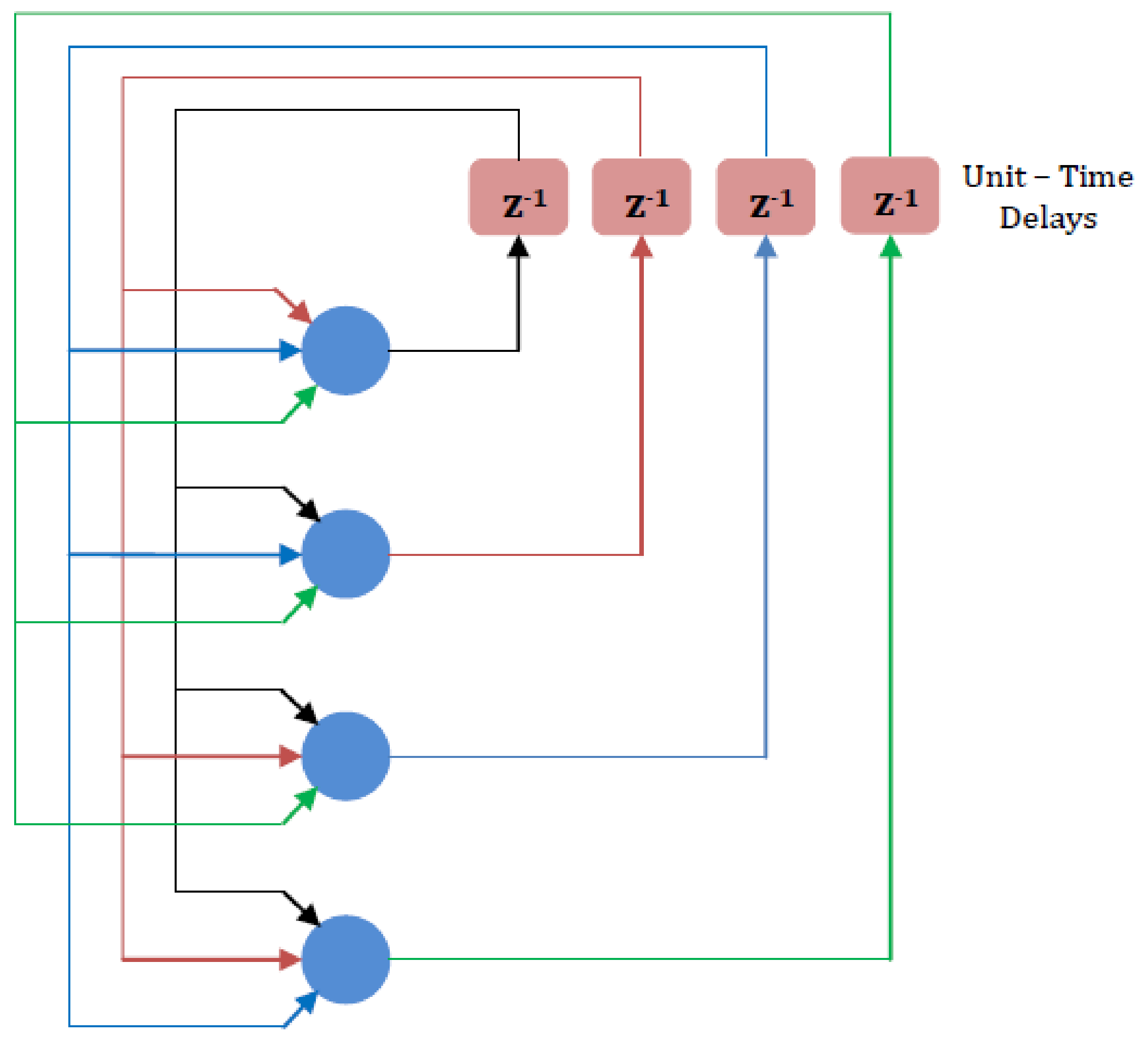
- Recurrent Networks
- ⮚
- Initialize weights randomly (for example ~N(0, σ2))
- ⮚
- Loop until convergence
- ⮚
- Compute the gradient
- ⮚
- Update the weights according to the equation:
- ⮚
- Return weights
3. Algorithm Description
- ⮚
- Symmetric sigmoid
- ⮚
- Logarithmic sigmoid
- ⮚
- Elliot sigmoid
- ⮚
- Soft max
- ⮚
- Linear
- ⮚
- Levenberg-Marquardt
- ⮚
- Bayesian Regularization
- ⮚
- BFGS Quasi-Newton
- ⮚
- Resilient Backpropagation
- ⮚
- Scaled Conjugate Gradient
- ⮚
- Conjugate Gradient with Powell/Beale Restarts
- ⮚
- Fletcher-Powell Conjugate Gradient
- ⮚
- Polak-Ribiére Conjugate Gradient
- ⮚
- One Step Secant
- ⮚
- Variable Learning Rate Gradient Descent
- ⮚
- Gradient Descent with Momentum
- ⮚
- Gradient Descent
4. Results
5. Conclusions
Author Contributions
Funding
Data Availability Statement
Conflicts of Interest
References
- Aziz, S.; Peng, J.; Wang, H.; Jiang, H. Admm-based distributed optimization of hybrid mtdc-ac grid for determining smooth operation point. IEEE Access 2019, 7, 74238–74247. [Google Scholar] [CrossRef]
- US. Department of the Interior Bureau of Reclamation. Transformers: Basics, Maintenance, and Diagnostics; U.S. Department of the Interior Bureau of Reclamation: Denver, CO, USA, 2005.
- Cigre Working Group. Guide for Transformer Maintenance—Cigre Working Group A2.34; Cigre: Paris, France, 2001; ISBN 978-2-85873-134-3. [Google Scholar]
- Kanno, M.; Oota, N.; Suzuki, T.; Ishii, T. Changes in ECT and dielectric dissipation factor of insulating oils due to aging in oxygen. IEEE Trans. Dielectr. Electr. Insul. 2001, 8, 1048–1053. [Google Scholar] [CrossRef]
- Aslam, M.; Arbab, M.N.; Basit, A.; Ahmad, T.; Aamir, M. A review on fault detection and condition monitoring of power transformer. Int. J. Adv. Appl. Sci. 2019, 6, 100–110. [Google Scholar]
- Patel, D.M.K.; Patel, D.A.M. Simulation and analysis of dga analysis for power transformer using advanced control methods. Asian J. Converg. Technol. 2021, 7, 102–109. [Google Scholar] [CrossRef]
- Siva Sarma, D.V.S.S.; Kalyani, G.N.S. ANN approach for condition monitoring of power transformers using DGA. In Proceedings of the IEEE Region 10 Conference TENCON, Chiang Mai, Thailand, 24 November 2004. [Google Scholar] [CrossRef]
- Hashemnia, N.; Islam, S. Condition assessment of power transformer bushing using SFRA and DGA as auxiliary tools. In Proceedings of the IEEE International Conference on Power System Technology (POWERCON), Wollongong, NSW, Australia, 28 September–1 October 2016. [Google Scholar] [CrossRef]
- Nemeth, B.; Laboncz, S.; Kiss, I. Condition monitoring of power transformers using DGA and Fuzzy logic. In Proceedings of the IEEE Electrical Insulation Conference, Montreal, QC, Canada, 31 May–3 June 2009. [Google Scholar] [CrossRef]
- Aciu, A.-M.; Nicola, C.-I.; Nicola, M.; Nițu, M.-C. Complementary Analysis for DGA Based on Duval Methods and Furan Compounds Using Artificial Neural Networks. Energies 2021, 14, 588. [Google Scholar] [CrossRef]
- Chatterjee, A.; Roy, N. Health Monitoring of Power Transformers by Dissolved Gas Analysis using Regression Method and Study the Effect of Filtration on Oil. Int. J. Electr. Comput. Eng. 2009, 3, 1903–1908. [Google Scholar]
- Dhini, A.; Faqih, A.; Kusumoputro, B.; Surjandari, I.; Kusiak, A. Data-driven Fault Diagnosis of Power Transformers using Dissolved Gas Analysis (DGA). Int. J. Technol. 2020, 11, 388–399. [Google Scholar] [CrossRef]
- Papadopoulos, A.E.; Psomopoulos, C.S. The contribution of dissolved gas analysis as a diagnostic tool for the evaluation of the corrosive sulphur activity in oil insulated traction transformers. In Proceedings of the 6TH IET Conference on Railway Condition Monitoring (RCM), University of Birmingham, Birmingham, UK, 17–18 September 2014. [Google Scholar]
- Papadopoulos, A.E.; Psomopoulos, C.S.; Kaminaris, S.D. Evaluation of the insulation condition of the two ONAN transformers of PUAS. In Proceedings of the International Scientific Conference eRA-10, Piraeus, Greece, 23–25 September 2015; pp. 1–7. [Google Scholar]
- Papadopoulos, A.; Psomopoulos, C.S. Dissolved Gas Analysis for the Evaluation of the Corrosive Sulphur activity in Oil Insulated Power Transformers. In Proceedings of the 9th Mediterranean Conference and Exhibition on Power Generation, Transmission and Distribution, IET (MedPower 2014), Athens, Greece, 2–5 November 2014. [Google Scholar]
- Huang, Y.-C.; Yang, H.-T.; Huang, C.-L. Developing a new transformer fault diagnosis system through evolutionary fuzzy logic. IEEE Trans. Power Deliv. 1997, 12, 761–767. [Google Scholar] [CrossRef]
- Aziz, S.; Wang, H.; Liu, Y.; Peng, J.; Jiang, H. Variable Universe Fuzzy Logic-Based Hybrid LFC Control With Real-Time Implementation. IEEE Access 2019, 7, 25535–25546. [Google Scholar] [CrossRef]
- Zhang, R.; Li, G.; Bu, S.; Aziz, S.; Qureshi, R. Data-driven cooperative trading framework for a risk-constrained wind integrated power system considering market uncertainties. Int. J. Electr. Power Energy Syst. 2023, 144, 108566. [Google Scholar] [CrossRef]
- IEEE DataPort. Available online: https://ieee-dataport.org/documents/dissolved-gas-data-transformer-oil-fault-diagnosis-power-transformers-membership-degree#files (accessed on 6 June 2022).
- Russell, S.J.; Norvig, P. Artificial Intelligence: A Modern Approach; Prentice Hall: Prentice, NJ, USA, 1995. [Google Scholar]
- Paluszek, M.; Thomas, S. MATLAB Machine Learning; Apress: Newark, NJ, USA, 2017. [Google Scholar]
- Mathworks. Available online: https://www.mathworks.com/content/dam/mathworks/mathworks-dot-com/campaigns/portals/files/machine-learning-resource/machine-learning-with-matlab.pdf (accessed on 10 July 2022).
- Sarajcev, P.; Kunac, A.; Petrovic, G.; Despalatovic, M. Artificial Intelligence Techniques for Power System Transient Stability Assessment. Energies 2022, 15, 507. [Google Scholar] [CrossRef]
- Ambare, V.; Uphad, Y.; Tikar, S.; Rabade, N.; Ingle, N. Literature Review on Artificial Intelligence. Int. J. Future Revolut. Comput. Sci. Commun. Eng. 2019, 5, 1–4. [Google Scholar]
- Haykin, S. Neural Networks and Learning Machines, 3rd ed.; Pearson Prentice Hall: Prentice, NJ, USA, 2008. [Google Scholar]
- Nanni, L.; Brahnam, S.; Paci, M.; Ghidoni, S. Comparison of Different Convolutional Neural Network Activation Functions and Methods for Building Ensembles for Small to Midsize Medical Data Sets. Sensors 2022, 22, 6129. [Google Scholar] [CrossRef] [PubMed]
- Ding, B.; Qian, H.; Zhou, J. Activation functions and their characteristics in deep neural networks. In Proceedings of the Chinese Control And Decision Conference (CCDC), Shenyang, China, 9–11 June 2018. [Google Scholar] [CrossRef]


| Function Name | Function |
|---|---|
| Threshold function | |
| Sigmoid function | |
| Tanh | |
| (Rectified Linear Unit) ReLU | |
| Leaky ReLU | where a small real number (e.g., 0.01) |
| Parametric Relu | where a real number |
| Exponential Linear Unit (ELU) | where a is a real number |
| Piecewise Linear Deformable Exponential Linear Unit (PDELU) | where a, t are real numbers. Parameter a controls the negative slope of function, and parameter t controls the degree of deformation |
| Swish | where parameter “β” is a learnable parameter |
| Mish | where parameter “a” is a learnable parameter |
| TanELU | where parameter “a” is a learnable parameter |
| S-shaped ReLU (SReLU) | where a is a real number and tl, tr, al and ar are four learnable parameters |
| Adaptive Piecewise Linear Unit (APLU) | where ac and bc are real numbers |
| Mexican ReLU (MeLU) | where k is the number of learnable parameters for each channel, cj are the learnable parameters, and c0 is the vector of parameters in PReLU |
| Gaussian ReLU (GaLU) | where k is the number of learnable parameters for each channel, cj are the learnable parameters, and c0 is he vector of parameters in PReLU |
| Soft Root Sign (SRS) | where α, β are nonnegative learnable parameters |
| Soft Learnable | where α and β are nonnegative trainable parameters |
| Splash | where αi, βi are learnable parameters |
| SoftMax | where n is the number of classes (possible outcomes) |
| Function Name | Expression |
|---|---|
| Quantifying Loss | |
| Empirical Loss | |
| Binary Cross Entropy Loss | |
| Mean Squared Error Loss |
| Training Algorithms | Transfer Functions | ||||
|---|---|---|---|---|---|
| Symmetric Sigmoid | Logarithmic Sigmoid | Elliot Sigmoid | Soft Max | Linear | |
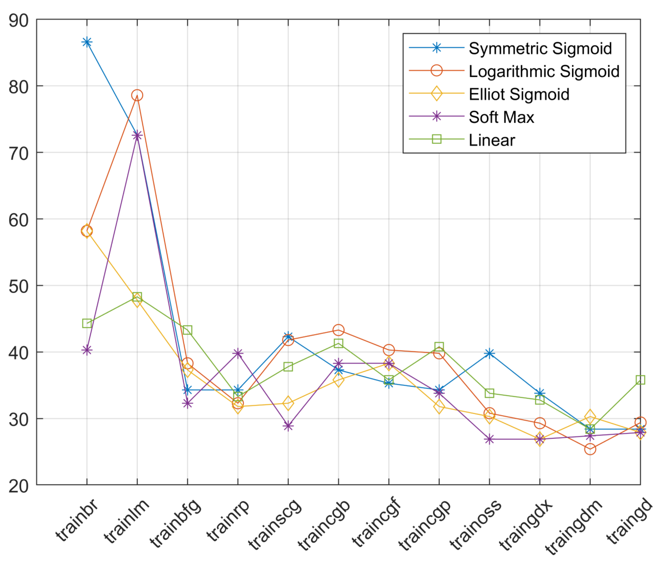
| trainbr | 86.6% | 58.2% | 58.2% | 40.3 | 44.3 |
| trainlm | 72.6% | 78.6% | 47.8% | 72.6 | 48.3 |
| trainbfg | 34.3% | 38.3% | 37.3% | 32.3 | 43.3 |
| trainrp | 34.3% | 32.3% | 31.8% | 39.8 | 33.3 |
| trainscg | 42.3% | 41.8% | 32.3% | 28.9 | 37.8 |
| traincgb | 37.3% | 43.3% | 35.8% | 38.3 | 41.3 |
| traincgf | 35.3% | 40.3% | 38.3% | 38.3 | 35.8 |
| traincgp | 34.3% | 39.8% | 31.8% | 33.8 | 40.8 |
| trainoss | 39.8% | 30.8% | 30.3% | 26.9 | 33.8 |
| traingdx | 33.8% | 29.3% | 26.9% | 26.9 | 32.8 |
| traingdm | 28.4% | 25.4% | 30.3% | 27.4 | 28.4 |
| traingd | 28.4% | 29.4% | 27.9% | 27.9 | 35.8 |
| Training Algorithm Acronym | Training Algorithm |
|---|---|
| trainbr | Bayesian Regularization |
| trainlm | Levenberg-Marquardt |
| trainbfg | BFGS Quasi-Newton |
| trainrp | Resilient Backpropagation |
| trainscg | Scaled Conjugate Gradient |
| traincgb | Conjugate Gradient with Powell/Beale Restarts |
| traincgf | Fletcher–Powell Conjugate Gradient |
| traincgp | Polak–Ribiére Conjugate Gradient |
| trainoss | One Step Secant |
| traingdx | Variable Learning Rate Gradient Descent |
| traingdm | Gradient Descent with Momentum |
| traingd | Gradient Descent |
| Training Algorithms | Transfer Functions | ||||
|---|---|---|---|---|---|
| Symmetric Sigmoid | Logarithmic Sigmoid | Elliot Sigmoid | Soft Max | Linear | |
| trainbr | 2/(5,5) | 1/(5) | 1/(5) | 1/(5) | 2/(5,5) |
| trainlm | 1/(5) | 1/(5) | 1/(5) | 2/(5,5) | 1/(5) |
| trainbfg | 1/(5) | 1/(5) | 1/(5) | 1/(5) | 1/(5) |
| trainrp | 1/(5) | 1/(5) | 1/(5) | 2/(5,5) | 1/(5) |
| trainscg | 1/(5) | 1/(5) | 1/(5) | 1/(5) | 1/(5) |
| traincgb | 1/(5) | 1/(5) | 1/(5) | 1/(5) | 2/(5,5) |
| traincgf | 2/(5,5) | 1/(5) | 2/(5,5) | 1/(5) | 1/(5) |
| traincgp | 1/(5) | 1/(5) | 1/(5) | 1/(5) | 1/(5) |
| trainoss | 1/(5) | 1/(5) | 1/(5) | 1/(5) | 1/(5) |
| traingdx | 1/(5) | 1/(5) | 1/(5) | 1/(5) | 1/(5) |
| traingdm | 1/(5) | 1/(5) | 1/(5) | 1/(5) | 1/(5) |
| traingd | 1/(5) | 1/(5) | 1/(5) | 1/(5) | 2/(5,5) |
| Training Algorithms | Transfer Functions | |||||
|---|---|---|---|---|---|---|
| Symmetric Sigmoid | Logarithmic Sigmoid | Soft Max | ||||
| Efficiency | NN Architecture | Efficiency | NN Architecture | Efficiency | NN Architecture | |
| trainbr | 86.6% | 2/(5,5) | 58.2% | 1/(5) | 40.3% | 1/(5) |
| trainlm | 72.6% | 1/(5) | 78.6% | 1/(5) | 72.6% | 2/(5,5) |
Disclaimer/Publisher’s Note: The statements, opinions and data contained in all publications are solely those of the individual author(s) and contributor(s) and not of MDPI and/or the editor(s). MDPI and/or the editor(s) disclaim responsibility for any injury to people or property resulting from any ideas, methods, instructions or products referred to in the content. |
© 2022 by the authors. Licensee MDPI, Basel, Switzerland. This article is an open access article distributed under the terms and conditions of the Creative Commons Attribution (CC BY) license (https://creativecommons.org/licenses/by/4.0/).
Share and Cite
Barkas, D.A.; Kaminaris, S.D.; Kalkanis, K.K.; Ioannidis, G.C.; Psomopoulos, C.S. Condition Assessment of Power Transformers through DGA Measurements Evaluation Using Adaptive Algorithms and Deep Learning. Energies 2023, 16, 54. https://doi.org/10.3390/en16010054
Barkas DA, Kaminaris SD, Kalkanis KK, Ioannidis GC, Psomopoulos CS. Condition Assessment of Power Transformers through DGA Measurements Evaluation Using Adaptive Algorithms and Deep Learning. Energies. 2023; 16(1):54. https://doi.org/10.3390/en16010054
Chicago/Turabian StyleBarkas, Dimitris A., Stavros D. Kaminaris, Konstantinos K. Kalkanis, George Ch. Ioannidis, and Constantinos S. Psomopoulos. 2023. "Condition Assessment of Power Transformers through DGA Measurements Evaluation Using Adaptive Algorithms and Deep Learning" Energies 16, no. 1: 54. https://doi.org/10.3390/en16010054
APA StyleBarkas, D. A., Kaminaris, S. D., Kalkanis, K. K., Ioannidis, G. C., & Psomopoulos, C. S. (2023). Condition Assessment of Power Transformers through DGA Measurements Evaluation Using Adaptive Algorithms and Deep Learning. Energies, 16(1), 54. https://doi.org/10.3390/en16010054