Using Machine Learning to Predict Multiphase Flow through Complex Fractures

Abstract

Multiphase flow properties of fractures are important in engineering applications such as hydraulic fracturing, evaluating the sealing capacity of caprocks, and the productivity of hydrocarbon-bearing tight rocks. Due to the computational requirements of high fidelity simulations, investigations of flow and transport through fractures typically rely on simplified assumptions applied to large fracture networks. These simplifications ignore the effect of pore-scale capillary phenomena and 3D realistic fracture morphology (for instance, tortuosity, contact points, and crevasses) that lead to macro-scale effective transport properties. The effect of these properties can be studied through lattice Boltzmann simulations, but they require high performance computing clusters and are generally limited in their domain size. In this work, we develop a technique to represent 3D fracture geometries and fluid distributions in 2D without losing any information. Using this innovative approach, we present a specialized machine learning model which only requires a few simulations for training but still accurately predicts fluid flow through 3D fractures. We demonstrate our technique using simulations of a water filled fracture being displaced by supercritical CO${}_2$. By generating highly efficient simulations of micro-scale multiphase flow in fractures, we hope to investigate a wide range of fracture types and generalize our method to be incorporated into larger discrete fracture network simulations.

1. Introduction

Fractures are ubiquitous in the subsurface and serve as preferential channels for flow and transport. This is because fractures may have permeability which is several orders of magnitude higher than the porous matrix of their host rock. Nevertheless, characterizing how multiple fluids travel through fractures is not well understood. This is mainly due to the fact that characterizing fluids during controlled experiments in the laboratory is very difficult and high fidelity simulations are computationally expensive. Often, reservoir engineers use simplifying assumptions of multiphase flow in a fractured system, such as no residual fluid saturation after drainage, very simple capillary pressure curves, and relative permeability that varies monotonically with fluid saturation. These assumptions result in significant inaccuracies of the system’s behavior.

The flow of two immiscible fluids through a fracture is controlled by many factors including the fracture geometry, fluid properties, pressure gradient, and the fluid-solid interfacial tension (also known as wettability) [1,2,3,4]. To study these systems, pore-scale simulations of multiphase flow can be carried out. The lattice-Boltzmann method (LBM) is a popular technique which is able to implement fluid-solid interactions and can simulate complex geometries. The LBM is also able to accurately capture the interfacial tension between fluids and different fluids viscosity ratios with ease. However, LBM simulations generally require high-performance computing resources (supercomputers) and long compute times which leads to small domains (on the order of 10 cms). Still, if enough simulations are performed, constitutive relationships for the system of interest can be derived.

The LBM has precedence in the literature for being used to investigate fractures [5,6,7,8,9,10,11]. The LBM has been shown to accurately honor the matrix-fluid transfer in a glass fracture by Landry et al. [9] who tested the method in a water-wet, oil-wet, and mixed-wet fracture observed with X-ray computed tomography. However, they hypothesized the need for a much finer computational grid since they could not recreate the irreducible water saturation. Additionally, Dou et al. (2013) [5] examined various contact angle scenarios and used incremental pressure to simulate displacement in a homogeneously wet, self-affine fracture. Although the flow field was similar across fractures due to homogeneous wetting conditions, they showed that the effective interfacial area was significantly affected over time by different magnitudes of wetting. Santos et al. (2018) [10] established that an effective size of heterogeneities (roughness and wetting patches) exists which modifies flow behavior by inducing fingering or preferential channeling. Guiltinan et al. (2020) [12] demonstrated the control of heterogeneous wetting distributions on residual saturation, breakthrough time, and relative permeability of rough fractures during drainage. Based on previous work, LBM investigations of multiphase flow in various fractures are potentially important, but the computational resources required by these simulations make a broader application of the work elusive. Preliminary work by Guiltinan et al. [13] investigated the possibility of employing neural networks to predict the 2D saturation of an invading fluid inside a fracture. Nevertheless, this model was limited to predicting the saturation at breakthrough as a 2D map at a given time-step, which oversimplifies the complexity of a moving plume in 3D.

A proxy model that could output accurate fluid distributions in complex fractures would be of great value for investigating correlations that relate fracture geometry with irreducible water saturation and relative permeability. Machine learning models, such as convolutional neural networks, have shown promise as a tool to train models that are more accurate than established techniques, and are much faster than full-physics simulations. In the context of flow at the micron-scale, machine learning models have been utilized to learn highly non-linear relationships in complex tasks. In particular, it has been shown that a neural network can learn the mapping function between 3D pore structure and fluid velocity [14,15,16,17], effective diffusivity [18], particle transport [19], and concentration fields [20] under steady-sate conditions. These machine learning proxy models can be utilized in-lieu of analytical solutions that only take in account effective properties and overlook the complex topological distribution of the domains. Even when trained machine learning models could output the effective property of interest with very good accuracy, high pixel-wise errors could appear, as an artifact of the sample being far from the training data or not knowing the physics. Nevertheless, it has been shown that these errors can be fixed by a simulator which can converge many orders of magnitude faster [21] compared to a full-physics simulation starting from scratch. Furthermore, Chang et al. [22] showed that a neural network prediction will always provide a better start point for a simulation which in turn will drop the compute time by a wide margin.

Nevertheless, multiphase flow applications have not been proposed at this scale due to the inherent dynamic time-complexities and GPU memory requirements that training requires. Another hurdle for applying machine learning models in physical contexts is that off-the-shelf models might not work well since they are not conceived to honor physical properties that are desirable in the context of interest. Due to these reasons, we propose a model that provides accurate predictions thanks to its internal structure and a loss function that takes into account the phase distributions. To the best of our knowledge, this paper presents the first methodology to train machine learning models on time-dependent unsteady multiphase flow simulations in porous media. In this paper, we introduce a data processing algorithm to compress multiphase fracture simulations and a specialized convolutional neural network architecture to learn from drainage simulations. We train a model to learn the mapping between a 3D fracture geometry and the corresponding response through time of a drainage front.

2. Data

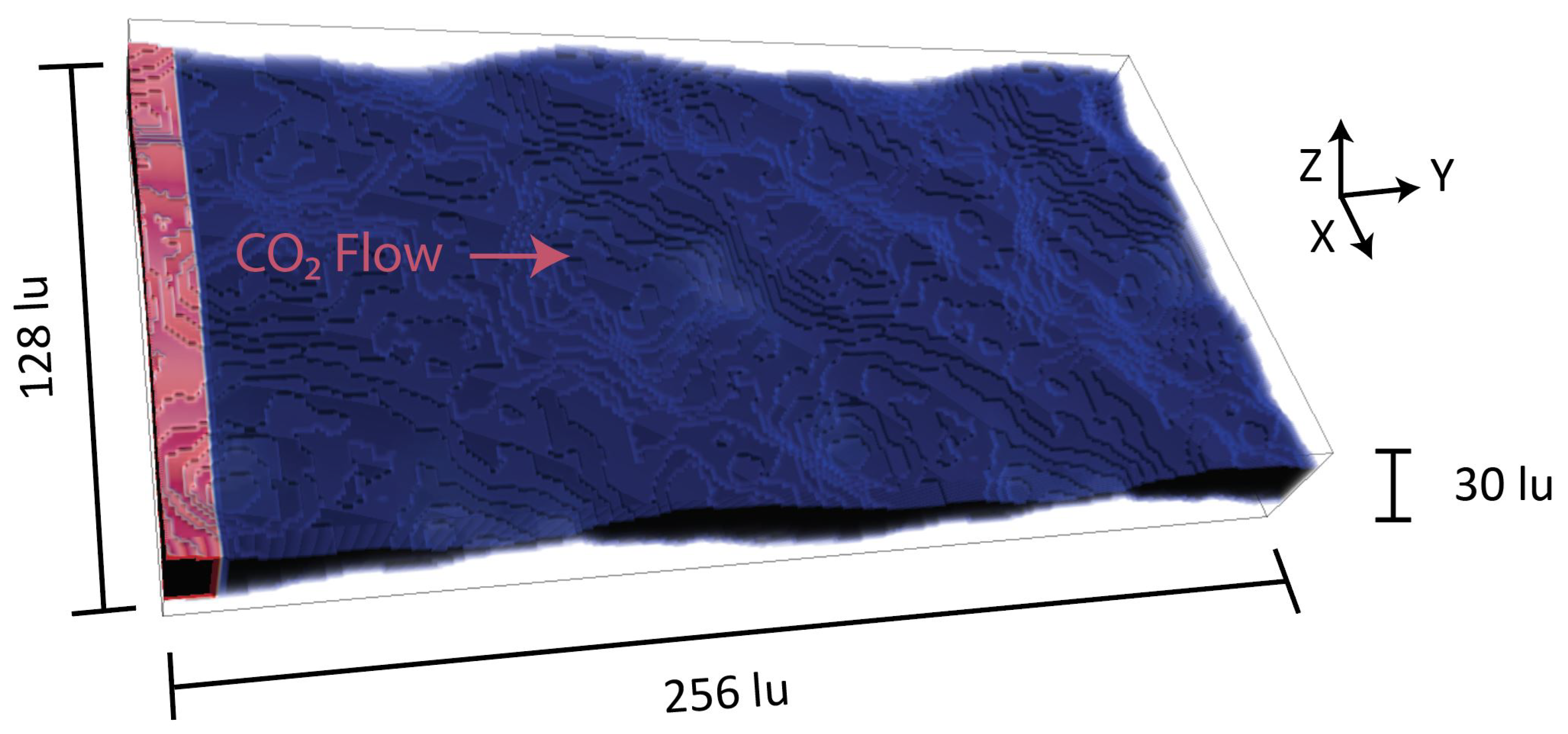
2.1. Physics Based Simulations

Our simulation was conducted with Taxila [23] which implements the multicomponent interparticle-potential Shan-Chen (SC) model [24,25] with some improvements as shown in Porter et al. [26] and Yu et al. [27]. These improvements target several weaknesses of the first SC model, including equilibrium densities that are viscosity dependent, numerical instabilities for certain kinematic viscosity ratios, and the presence of large, spurious currents near interfaces. We use the D3Q19-MRT model in this work, or the multiple relaxation time version of the three-dimensional model, with eight orders of isotropy enforced. This model is a three-dimensional mesh in which there are 18 different velocities leaving from each node, in addition to one stationary “velocity” representing no movement. Each fracture was generated using the synthetic fracture generation software SynFrac [28] and the Glover method [29,30]. For more details on the the fracture creation and simulations see Guiltinan et al. [11].

The model domain is 128 × 256 × 30 lattice units (lu) (Figure 1). Relaxation times are chosen for the red and blue fluid to create the viscosity ratio of supercritical CO${}_2$ (s-CO${}_2$) and water. The red fluid represents s-CO${}_2$, which is initialized to fill the first 10 lattice units in the y-direction. Our boundary conditions consist of a water saturated s-CO${}_2$ constant pressure at the inlet (y = 0) which drives drives the s-CO${}_2$ across the model domain to a constant pressure at the outlet. At the outlet (y = 256) there is a thin layer of water held at a constant pressure which the s-CO${}_2$ is attempting to displace. This avoids capillary pressure effects and maintains a constant 500 Pa differential pressure across the domain. In the x-direction the model is periodic, meaning when fluid flows across x = 128 it reappears at x = 0. At the fracture surface a bounce back condition is implemented with an adhesive force applied to the water and a repulsive force applied to the s-CO${}_2$. These forces amount to a contact angle of approximately 30° and represent a water wetting fracture. For more information on these forces and the simulation setup see Guiltinan et al. [11]. Each simulation took approximately 3600 CPU-hours and was completed utilizing the high performance computing resources at Los Alamos National Lab. Every 1000 time steps the density fields for the s-CO${}_2$ and water were saved as 3D fields, which yield approximately 100 checkpoints per simulation. The LBM simulation setup is illustrated in Figure 1.

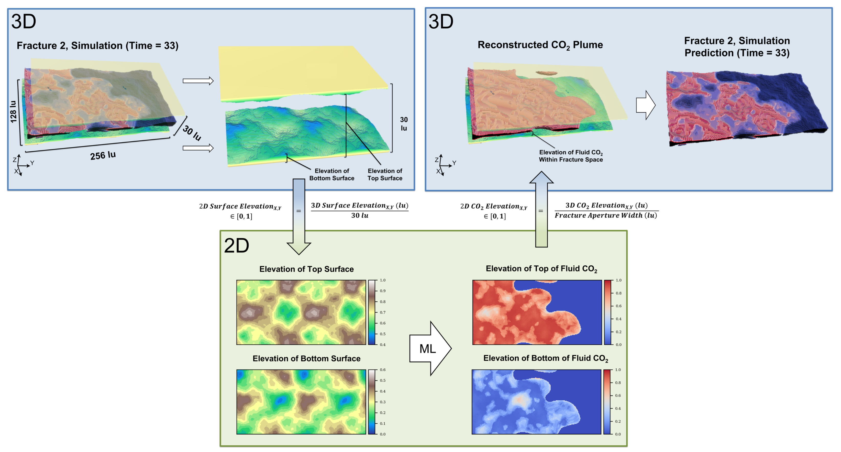
2.2. Data Processing

A novel approach allows for the representation of a 3D fracture in 2D without any information loss, making machine learning models on unsteady state multiphase flow simulations tractable. We propose a workflow to project the 3D time-dependent data into 2D arrays. First, the 3D fracture domain is projected into two 2D arrays that each represent the elevations of the top and bottom surfaces of the fracture, which are then normalized from zero to one with respect to the domain size. Contact points (where the top and bottom surfaces are in contact) are represented by the same value in both arrays. The top and bottom surfaces of the fracture geometry act as inputs to our proposed machine learning model.

Next, each time step of the simulations is projected into two 2D arrays representing the elevations of the top and the bottom of the CO${}_2$ plume at that time step. These are normalized with respect to the size of the fracture aperture. These elevation maps of the CO${}_2$ serve as the targets for our model predictions. This process serves two purposes: (1) compressing the spatial complexity by a factor of the domain length in the z-axis, and (2) constraining the predictions of the machine learning model. Since the prediction targets range from zero to one, the predictions of the model will always stay within the fracture surfaces, so no fluid will be predicted outside the fracture. This is also a hard constraint in our model.

The full workflow projecting the 3D simulation data into 2D arrays and then reconstructing the simulations from the model predictions is shown below in Figure 2 and Algorithm 1.

By expressing the 3D simulation data in terms of the positions of the fracture surfaces and the CO${}_2$ plume, the dataset is compressed by a significant factor, and the 3D simulation can still be reconstructed without information loss (with an accuracy of 99.99%). It is worth noting that training a three-dimensional deep neural network for this task would be intractable given the domain size and number of time-steps.

Algorithm 1 3D to 2D fracture conversion.

Input: A 3D array $F_t$ of shape (X, Y, Z) representing a simulation in a fracture F at time t, where $F_t\left[i\right]\left[j\right]\left[k\right]$ represents the value of the voxel at index $(i,j,k)$ in the array such that $0\le i<X$, $0\le j<Y$, and $0\le k<Z$. Each voxel’s value is an integer that represents either $C{O}_2$ (2), brine (1), or the solid rock surrounding the fracture (0). Output: A 3D array $P_t$ of shape (X, Y, Z) representing the predicted simulation P in fracture F at time t.

▹ Convert 3D simulation to top and bottom fracture surfaces in 2D. $T_{Fracture}$, 2D elevation of top surface of the solid fracture $B_{Fracture}$, 2D elevation of bottom surface of the solid fracture fori in 0 … X, j in 0 … Y do:     for k in 0 … Z - 1 do:         if $F_t$[i][j][k] == 0 and $F_t$[i][j][k + 1] > 0 then            $B_{Fracture}\left[i\right]\left[j\right]\leftarrow k$        ▹ found top edge of bottom fracture surface         end if         if $F_t$[i][j][k] > 0 and $F_t$[i][j][k + 1] == 0 then            $T_{Fracture}\left[i\right]\left[j\right]\leftarrow k+1$    ▹ found bottom edge of top fracture surface         end if     end for end for

▹ Obtain predicted position of the top and bottom surfaces of fluid $C{O}_2$. $T_{C{O}_2},B_{C{O}_2}\leftarrow ML\left(\frac{T_{Fracture}}{Z},\frac{B_{Fracture}}{Z}\right)$

▹ Interpret predicted $C{O}_2$ surfaces as fractions of the aperture. T’${}_{C{O}_2}\leftarrow B$’${}_{Fracture}+T_{C{O}_2}\ast (T_{Fracture}-B_{Fracture})$ B’${}_{C{O}_2}\leftarrow B$’${}_{Fracture}+B_{C{O}_2}\ast (T_{Fracture}-B_{Fracture})$

▹ Convert 2D predictions to 3D simulation. $P_t$, 3D predicted simulation fori in 0 … X, j in 0 … Y do:     for k in 0 … Z do:         if $B_{C{O}_2}^{\prime }\le k\le T_{C{O}_2}^{\prime }$ then            $P_t\left[i\right]\left[j\right]\left[k\right]\leftarrow 2$         else            if $B_{Fracture}\le k\le T_{Fracture}$ then                $P_t\left[i\right]\left[j\right]\left[k\right]\leftarrow 1$            else                $P_t\left[i\right]\left[j\right]\left[k\right]\leftarrow 0$            end if         end if     end for end for

To train our machine learning model, we selected simulations of twelve unique fractures which encompass the main flow features that we want our model to learn–for instance different mean apertures and roughness (four of these are illustrated in Figure 3). The roughness’ fractal dimension varies from 2.1 to 2.5 and the mean aperture from 10 to 20 lattice-units. These conditions span enough of the physical space that we would like our ML model to understand. We use a training set consisting of ten fractures that are used to fit the model’s parameters, and we withhold the remaining two fractures from the dataset as a testing set to evaluate the accuracy of the model’s predictions on unseen fractures after training.

3. Machine Learning Model

For the purpose of our work, we developed a convolutional neural network to learn a mapping between the morphology of a 3D fracture and the position of the injected supercritical CO${}_2$ at different time steps throughout the lattice-Boltzmann simulation. A convolutional network is chosen over other machine learning models due to its proven effectiveness in image processing tasks such as ours, as well as its versatility and ease of implementation compared to models such as transformers, which require large amounts of data and millions of learnable parameters. Convolutional neural networks are well-suited for this task since fractures are spatially correlated at different length-scales so the convolutional kernels can learn how different aperture features impact flow throughout these channels. The following subsections will describe the intuition behind our neural network architecture, loss function, and training procedure.

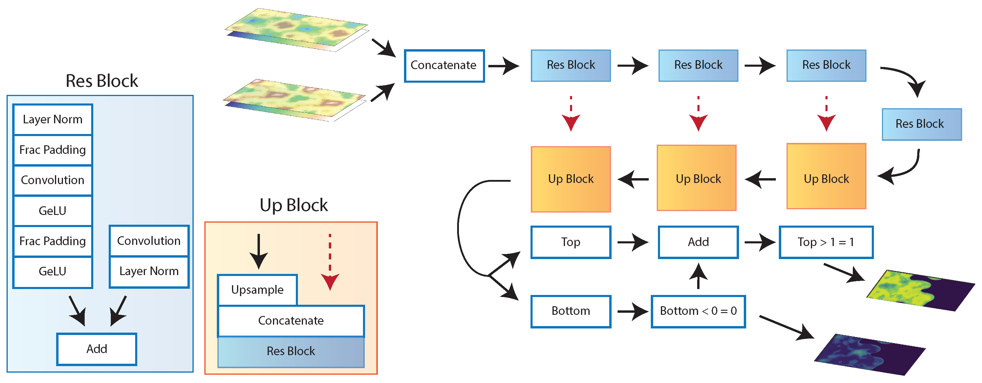
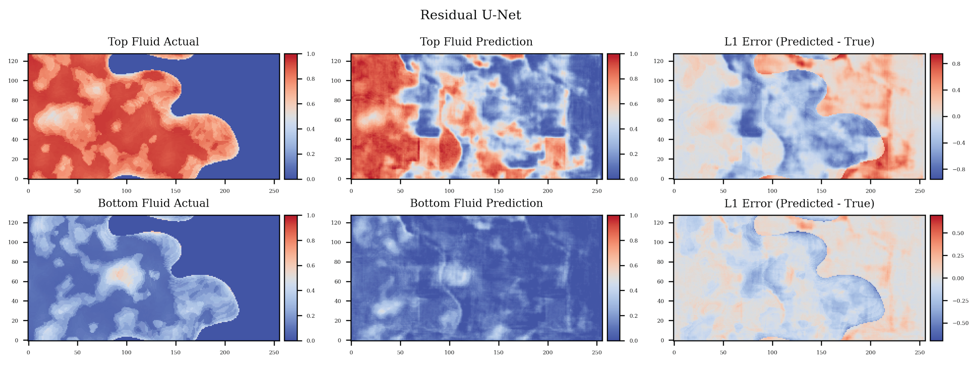
3.1. Network Architecture Development

Convolutional neural networks (ConvNets) have shown an exceptional ability to learn intricate mappings in image to image problems. Rather than use a normal matrix multiplication (i.e., multilayer perceptrons), they utilize convolution operations to learn spatial patterns locally across the image. ConvNets make use of kernels that capture interactions of neighboring pixels, and by sliding these kernels across the image, they efficiently gather important information with regards to the domain, aiming to reconstruct the output of interest. By stacking a series of convolutional layers, a ConvNet is able to learn features at numerous levels of abstraction, progressively widening its field of vision. Moreover, a notable feature is that with respect to translation, convolution layers are equivariant. This means that translating, or shifting, an input feature will result in the output of the convolutional layer also being shifted by that amount. This allows for inputs–in our case, fractures–to be of varying size, which is useful in tasks relating to pattern recognition. Using these structures, networks can be trained to recognize patterns between image inputs and outputs that are non-linear and complex.

In the context of network architecture development, it has been shown that the performance of a network can benefit from increasing its depth (or in other words, to stack more layers) [31]. This is partly due to the fact that deeper networks have a wider field of vision, so they can learn semantically more meaningful features across the domain.

Aside from being more computationally expensive, deep networks can be harder to train because of issues such as exploding or vanishing gradients. He et al. [32] presented the residual network (ResNet) to improve gradient flow. By concatenating the the input of a convolutional layer stack to its output in a “residual connection”, the ResNet creates better pathwasy for gradient flow, easing the training of deeper networks. Another issue with deep networks is that portions of the input could be valuable information for the target prediction, but are lost when traveling across many layers. To overcome this hurdle, Ronneberger et al. [33] presented the U-Net, which refines reconstruction of the target output by concatenating the feature maps at certain points from the encoder to the decoder. In this way, the network’s structure preserves information about both low-level features, such as edges or lines, and high-level features, such as recognizable objects. This is relevant in the context of fractures, because features like contact points do not get flow pass them. Carrying on from the improvements made by these two architectures, Zhang [34] proposed a Deep Residual U-Net (ResUNet). This network, which used both residual units and skip connections between them, achieved accurate results with a small training set and an efficient amount of parameters, and was also easily trained when compared to the previous U-Net, which required either a pre-trained model or substantial augmentation in the training data.

In this work, we present a specialized model that is a modification of the ResUNet. We choose to modify a Residual U-net for two reasons: (1) the skip connections between the encoding and decoding branches benefit the model by preserving information from the original morphology of the fracture, which affects the final shape of the CO${}_2$ plume; and (2) residual units have been shown to enhance training and address issues with deeper networks such as vanishing and exploding gradients. Our model is a novel combination of physically accurate input features, modern neural network design choices, physical constraints, and a specially designed loss function that considers fluid dynamics. Thus, it is tailored specifically for predicting multiphase fluid distribution in fractures.

The input to the encoder branch consists of 2D arrays representing the top and bottom surfaces of the fracture geometry. To honor the boundary conditions of the problem during convolutional neural network processing, we add additional padding values that expand the size of the arrays in each direction. In the x-direction, padding values are periodic and repeat in a cycle. In the y-direction, padding values mirror the values at each edge of the array. These arrays are then combined with a linear distance feature that provides additional spatial information. This additional input is a 2D array of uniformly increasing values from left to right, normalized to be between 0 and 1, which represent the distance of each point from the inlet of the fracture. The top and bottom surfaces of the fracture are each combined with the distance feature, creating four total channels in the input data as illustrated in Figure 4. This structure for the input data ensures that both the top and bottom surfaces are combined with the same distance feature when we perform separate grouped convolutions on the two surfaces, which will be further explained in the following section.

The encoder performs convolutions on the input in a series of residual blocks. Each block consists of two convolutional layers with a stride of two and a residual connection as an additional pathway for the information flow (as shown in Figure 5). Each blocks compresses the image into an array of half the size of the input. We use grouped convolutions with two groups to separate the convolutions for the top and bottom surfaces of the input fracture, including the linear distance feature for each group. By passing information about the top and bottom surfaces of the solid fracture through distinct convolutional groups, we increase the computational efficiency of the network by neglecting connections with all the input features [35]. The input data is downsampled at each residual unit throughout the encoder, using a strided convolution [36]. The number of feature channels is doubled at each downsampling stage to add more latent information. In the fourth residual unit connecting the encoder to the decoder, no grouped convolutions are used, which allows mixing information across the feature channels so semantically meaningful features are allowed to travel from the top and bottom. This is also the unit with most feature maps, hence processing and abstracting capacity. Similarly, we have a decoding branch following the same group ordering as the decoder branch. The decoder performs convolutions with residual blocks, upsampling the data and using skip connections from the encoder to recover the position of the fluid CO${}_2$ in the same dimensions as the input.

We also implement new architectural design choices made in [37], which were shown to boost the performance of a standard ResNet by borrowing from modern Transformer architectures. One design change we adapt from Liu et al. [37] is using the GELU (Gaussian Error Linear Unit) [38] activation function following each convolutional layer. This not only increases performance, but stabilizes training. Another change we implemented is substituting BatchNormalization for LayerNormalization, reducing the normalization’s dependency on other fracture geometries in the batch. Following their recommendations, we also reduced the total number of activation and normalization layers per residual block. The full model architecture is illustrated in Figure 5.

To honor the physical properties of the problem, we add the predicted 2D map for the bottom CO${}_2$ fluid plume to the prediction of the top of the plume. This ensured that the top surface of the CO${}_2$ always lies above its bottom surface (as it occurs in the simulation). A ReLU activation function is applied to the bottom surface map to exclude illogical negative values, and the values of the top are clipped at 1, so there cannot be fluid predicted outside the fracture. These operations guarantee physical predictions and can be seen in Figure 5.

3.2. Loss Function

An important consideration in our model architecture is the structure of the loss function, or the function that quantifies the degree of error between the model’s prediction and the expected output. We use a pixel-wise mean squared error (MSE) between the prediction and the target, which both consist of 2D maps of the top and bottom surfaces of the fluid CO${}_2$, as one component in the loss function.

Although minimizing the MSE is effective during training and causes the model to converge, when training with solely MSE, we discovered that the pixels near the boundary between CO${}_2$ and brine (the front), were not precisely identified in our predictions. Instead, parts of the predicted CO${}_2$ bled into the brine, and the pixel values of the CO${}_2$ surrounding the front were inaccurate and inconsistent. In order to encourage the model towards predicting a sharper, more accurate boundary between the two fluid phases, we apply an additional weighting to the pixel-wise MSE: the calculated error for pixels contained within a certain range of the CO${}_2$-brine boundary, denoted by $M_i$, is multiplied by a weight $\lambda$, attributing more significance to those pixels in the prediction. The weight $\lambda$ is a constant that we set to 0.001.

Furthermore, using a pixel-wise MSE implies the assumption that the underlying data has been generated from a normal distribution–in Bayesian terms, this means we assume a Gaussian prior. However, our dataset can be classified into two categories, one for each fluid phase. This means that the categories are generated from a Bernoulli distribution, which is not currently considered in our loss function. Thus, we also use a binary cross-entropy loss in our model’s loss function for the two distinct phases in our simulation. This penalizes the network more heavily for incorrectly classifying the fluid phase, and helps to reduce noise in the output (for instance, we know that there should not be isolated spots CO${}_2$ within the brine in the fracture). During training, we observe that the cross-entropy term dominates the loss in the beginning, but as the network correctly identifies the two distinct phases, the training loss suddenly decreases and the MSE loss becomes more significant.

The full loss function for our network is shown in Equation (1) below:

$$\begin{array}{c}\hfill \mathcal{L}=\frac{1}{N_{pix}}\sum _{i=1}^{N_{pix}}(\\ \hfill \frac{{(y_{i,b}-{\widehat{y}}_{i,b})}^2}{{\overline{y}}_{train,b}}(1+\lambda M_i)& -(y_{i,b}>{ϵ}_b)log({\widehat{y}}_{i,b}>{ϵ}_b)+\hfill \\ \hfill \frac{{(y_{i,b}-({\widehat{y}}_{i,b}+max\left({\widehat{y}}_{i,t}\right),0))}^2}{{\overline{y}}_{train,t}}(1+\lambda M_i)& -(y_{i,t}>{ϵ}_t)log(({\widehat{y}}_{i,b}+max\left({\widehat{y}}_{i,t}\right),0)>{ϵ}_t)\hfill \\ \hfill & ),\hfill \end{array}$$

(1)

where $N_{pix}$ denotes the number of pixels of the fracture projection, y is the true value, $\widehat{y}$ the prediction of our model, and ${\overline{y}}_{train}$ the mean value of the training set. t and b denote the top and bottom menisci of the CO${}_2$. We calculate the pixel-wise MSE which is normalized by the mean value of the training set. This ensures that the error for the top and bottom surfaces of the CO${}_2$, despite having different magnitudes, are still weighted equally in the loss. For the additional weighting of pixels near the front, we choose two model hyperparameters that are fixed prior to training: $\lambda$, the weighting, and $M_i$, the range of pixels surrounding the front that the weighting is applied to. The values for these hyperparameters were tuned by testing different combinations of models and parameters while observing key performance indicators, such as the CO${}_2$ saturation accuracy and any visual improvements in the shape of the CO${}_2$ plume in 2D. The term in the binary cross-entropy loss, $ϵ$, denotes a minimum threshold for pixel values in the prediction. Since the prediction can contain many small pixel values close to zero, we choose a minimum threshold value for which all pixels below that value are considered to be zero, which in this context means that those pixels belong to the brine phase. As result, the binary cross-entropy is more tolerant of predicted values below $ϵ$ when comparing the predicted and actual fluid phase. Through experimental testing of our loss function, we choose $ϵ$ to be the minimum value in the target projection that is greater than zero.

3.3. Training

At training time, we additionally augment our dataset by reflecting the input and target arrays across the x and y axes, reversing the previously mentioned distance input for reflections across the y-axis. This process quadruples the size of our training set and enhances the predictive performance of the model by a wide margin. We set-up our model using the Tensorflow 2.10 deep learning library [39] and python 3.10. We train our model for 20,000 epochs with a mini-batch size of two samples and a learning rate of 1 × 10${}^{-4}$. Training the model requires 4 Gigabytes of memory and takes four hours to complete on a commercial GPU card using 32-bit precision training.

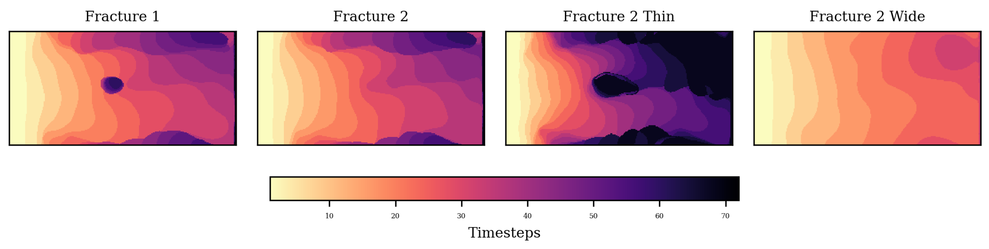
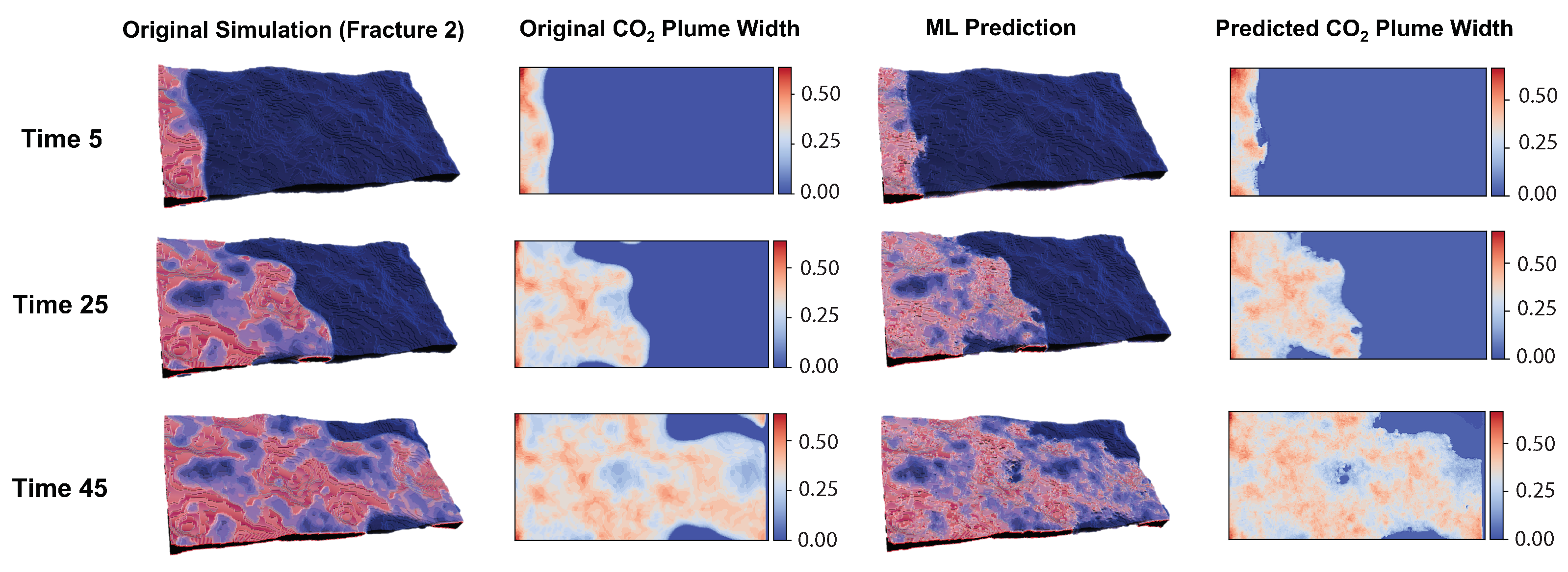
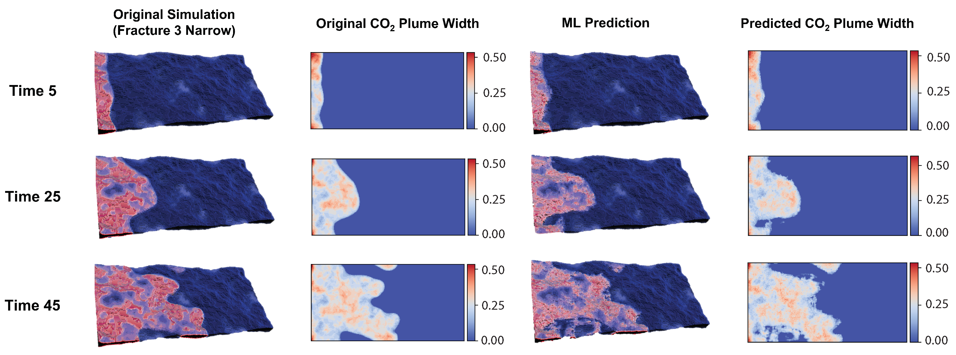
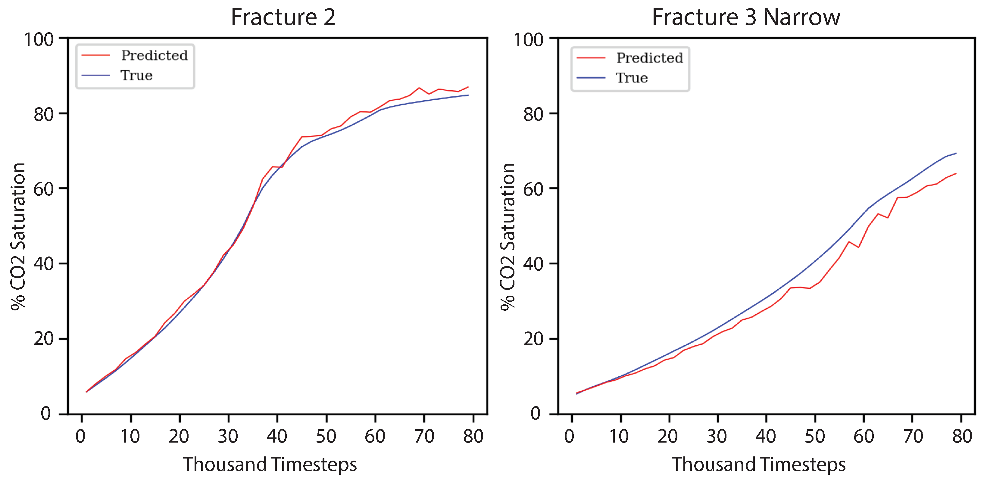
4. Results and Discussion

We tested our model using 40 timesteps from two fractures which had never been seen by the machine learning algorithm. Five of the simulation timesteps and the predictions of our model are shown in Figure 6 and Figure 7. In general the plume shape and phase distributions are accurately reproduced by the ML prediction. It is worth noting that the model is able to accurately capture the breakthrough time in widely different fractures, while some noise in the front is noted, the overall accuracy is very high and areas within the simulation with residually trapped brine are captured. In general, the algorithm predicts sharper interfaces than the simulation, but if these model outputs were used as an input into an LBM simulation, capillary forces would immediately smooth this result. In this way, a coupled LBM and machine learning scheme could be devised where the machine learning algorithm advances the front by approximately 20k timesteps, the LBM quickly resolves the interface over a few hundred timesteps, and then the process is repeated. This is similar to the work conducted by [21].

In addition to the phase distributions, the saturation with time is also faithfully reproduced in Figure 8. These predictions are critical to accurately developing relative permeability relationships for multiphase flow in fractures, an important parameter which is often ignored in larger scale simulations due to computational constraints and experimental difficulties [12]. In this example, the LBM simulations took approximately 3600 CPU-hours where the ML prediction takes less than a second for each new geometry. While it takes time to train on previous simulation data and develop algorithms, the end result makes 3D multiphase flow predictions in fractures with our applied boundary conditions nearly effortless.

The design of our neural network architecture was developed in stages, with new features being added to the model during each stage. These developments are shown in Figure 9, Figure 10 and Figure 11. Each model is trained for 16K epochs, and the predictions are shown for Fracture 2 at time step 33 in the testing set. Figure 9 presents the result of a baseline Res U-Net prediction trained on our dataset. Figure 10 shows the results of applying a linear feature which represents the distance from the source boundary condition on the left to the outlet boundary condition on the right. The application of this feature allows kernels of the neural network to understand their relative position with respect to the boundary conditions. Finally, Figure 11 presents the final result of our algorithm development using the loss section described in Section 3.2. The application of the mask makes the front sharper and removes disconnected features beyond the CO${}_2$ front. The binary cross entropy (BCE) loss reduces the noise in the brine phase.

5. Conclusions

Multiphase flow through fractures is important in a variety of engineering applications such as, production from hydraulic fractures, nuclear waste disposal performance assessment, CO${}_2$ sequestration caprock security, and geothermal energy projection. Often in these scenarios, fracture flow is the dominant feature controlling the response of interest for example, the decline curve during unconventional production, plume migration, or CO${}_2$ leakage across a caprock seal. However, commonly used numerical models ignore the complexity of real world fractures. Here we present a step towards investigating more realistic fractures through the pore-scale simulations of complex single fractures accelerated with machine learning. We demonstrate how a novel data processing algorithm and a specialized neural network architecture can provide fast and accurate predictions of the position of a moving front during CO${}_2$ injection for a given set of boundary conditions. Although local average errors are present in the output of the network, researchers have shown that this can be corrected with a few iterations of the full-physics simulation (as shown in [21,22]). Knowing the exact 3D fracture geometry present in a particular reservoir of interest is not a prerequisite for using our workflow. Often effective properties of fractures associated with certain reservoirs are well-known [30] and these can be used to create realizations of fracture surfaces that can be used to get fluid distributions using our proposed model.

For our future work, we are planning to create a large open access dataset of multiphase simulations with different fracture properties and simulation conditions, similar to what was achieved in [14]. This larger dataset will allow for the interrogation of the controlling parameters on multiphase flow through fractures. We hope that through the further development of our machine learning algorithms we will be able to bridge from the pore-scale to applicable scales for different engineering applications.

References

1. Guiltinan, E.J.; Cardenas, M.B.; Bennett, P.C.; Zhang, T.; Espinoza, D.N. The effect of organic matter and thermal maturity on the wettability of supercritical CO2 on organic shales. Int. J. Greenh. Gas Control 2017, 65, 15–22. [Google Scholar] [CrossRef]
2. Renshaw, C.E. On the relationship between mechanical and hydraulic apertures in rough-walled fractures. J. Geophys. Res. Solid Earth 1995, 100, 24629–24636. [Google Scholar] [CrossRef]
3. Vogler, D.; Settgast, R.R.; Annavarapu, C.; Madonna, C.; Bayer, P.; Amann, F. Experiments and Simulations of Fully Hydro-Mechanically Coupled Response of Rough Fractures Exposed to High-Pressure Fluid Injection. J. Geophys. Res. Solid Earth 2018, 123, 1186–1200. [Google Scholar] [CrossRef]
4. Wang, L.; Cardenas, M.B.; Slottke, D.T.; Ketcham, R.A.; Sharp, J.M. Modification of the Local Cubic Law of fracture flow for weak inertia, tortuosity, and roughness. Water Resour. Res. 2015, 51, 2064–2080. [Google Scholar] [CrossRef]
5. Dou, Z.; Zhou, Z.; Sleep, B.E. Influence of wettability on interfacial area during immiscible liquid invasion into a 3D self-affine rough fracture: Lattice Boltzmann simulations. Adv. Water Resour. 2013, 61, 1–11. [Google Scholar] [CrossRef]
6. Eker, E.; Akin, S. Lattice Boltzmann simulation of fluid flow in synthetic fractures. Transp. Porous Media 2006, 65, 363–384. [Google Scholar] [CrossRef] [Green Version]
7. Ju, Y.; Zhang, Q.; Zheng, J.; Chang, C.; Xie, H. Fractal model and Lattice Boltzmann Method for Characterization of Non-Darcy Flow in Rough Fractures. Sci. Rep. 2017, 7, 41380. [Google Scholar] [CrossRef] [PubMed] [Green Version]
8. Kim, I.; Lindquist, W.B.; Durham, W.B. Fracture flow simulation using a finite-difference lattice Boltzmann method. Phys. Rev. E Stat. Phys. Plasmas Fluids Relat. Interdiscip. Top. 2003, 67, 9. [Google Scholar] [CrossRef]
9. Landry, C.J.; Karpyn, Z.T.; Ayala, O. Relative permeability of homogenous-wet andmixed-wet porousmedia as determined by pore-scale lattice Boltzmann modeling. Water 2014, 50, 3672–3689. [Google Scholar] [CrossRef]
10. Santos, J.E. Lattice-Boltzmann Modeling of Multiphase Flow through Rough Heterogeneously Wet Fractures. Ph.D. Thesis, The University of Texas at Austin, Austin, TX, USA, 2018. [Google Scholar] [CrossRef]
11. Guiltinan, E.; Estrada Santos, J.; Kang, Q.; Cardenas, B.; Espinoza, D.N. Fractures with Variable Roughness and Wettability. 2020. Available online: https://www.digitalrocksportal.org/projects/314 (accessed on 10 October 2022).
12. Guiltinan, E.J.; Santos, J.E.; Cardenas, M.B.; Espinoza, D.N.; Kang, Q. Two-phase fluid flow properties of rough fractures with heterogeneous wettability: Analysis with lattice Boltzmann simulations. Water Resour. Res. 2020, 57, e2020WR027943. [Google Scholar] [CrossRef]
13. Guiltinan, E.; Santos, J.E.; Kang, Q. Residual Saturation During Multiphase Displacement in Heterogeneous Fractures with Novel Deep Learning Prediction. In Proceedings of the Unconventional Resources Technology Conference (URTeC), Online, 20–22 July 2020; Society of Petroleum Engineers (SPE): Austin, TX, USA, 2020. [Google Scholar] [CrossRef]
14. Zhou, X.H.; McClure, J.E.; Chen, C.; Xiao, H. Neural network-based pore flow field prediction in porous media using super resolution. Phys. Rev. Fluids 2022, 7, 074302. [Google Scholar] [CrossRef]
15. Santos, J.E.; Xu, D.; Jo, H.; Landry, C.J.; Prodanović, M.; Pyrcz, M.J. PoreFlow-Net: A 3D convolutional neural network to predict fluid flow through porous media. Adv. Water Resour. 2020, 138, 103539. [Google Scholar] [CrossRef]
16. Santos, J.E.; Yin, Y.; Jo, H.; Pan, W.; Kang, Q.; Viswanathan, H.S.; Prodanović, M.; Pyrcz, M.J.; Lubbers, N. Computationally Efficient Multiscale Neural Networks Applied to Fluid Flow in Complex 3D Porous Media. Transp. Porous Media 2021, 140, 241–272. [Google Scholar] [CrossRef]
17. Kashefi, A.; Mukerji, T. Point-cloud deep learning of porous media for permeability prediction. Phys. Fluids 2021, 33, 097109. [Google Scholar] [CrossRef]
18. Wang, H.; Yin, Y.; Hui, X.Y.; Bai, J.Q.; Qu, Z.G. Prediction of effective diffusivity of porous media using deep learning method based on sample structure information self-amplification. Energy AI 2020, 2, 100035. [Google Scholar] [CrossRef]
19. Marcato, A.; Boccardo, G.; Marchisio, D. A computational workflow to study particle transport and filtration in porous media: Coupling CFD and deep learning. Chem. Eng. J. 2021, 417, 128936. [Google Scholar] [CrossRef]
20. Marcato, A.; Estrada Santos, J.; Boccardo, G.; Viswanathan, H.; Marchisio, D.; Prodanović, M. Prediction of Local Concentration Fields in Porous Media with Chemical Reaction Using a Multi Scale Convolutional Neural Network. Chem. Eng. J. 2022, 140367. [Google Scholar] [CrossRef]
21. Wang, Y.D.; Chung, T.; Armstrong, R.T.; McClure, J.; Ramstad, T.; Mostaghimi, P. Accelerated Computation of Relative Permeability by Coupled Morphological and Direct Multiphase Flow Simulation. J. Comput. Phys. 2020, 401, 108966. [Google Scholar] [CrossRef]
22. Chang, B.; Santos, J.; Prodanovic, M. ElRock-Net: Assessing the Utility of Machine Learning to Initialize 3D Electric Potential Simulations; Society of Core Analysists: 2022. Available online: http://jgmaas.com/SCA/2022/SCA2022-11.pdf (accessed on 10 October 2022).
23. ecoon/Taxila-LBM: Lattice Boltzmann code from LANL. Available online: https://github.com/ecoon/Taxila-LBM (accessed on 10 October 2022).
24. Shan, X.; Chen, H. Lattice Boltzmann model for simulating flows with multiple phases and components. Phys. Rev. E 1993, 47, 1815–1819. [Google Scholar] [CrossRef] [Green Version]
25. Shan, X.; Chen, H. Simulation of nonideal gases and liquid-gas phase transitions by the lattice Boltzmann equation. Phys. Rev. E 1994, 49, 2941–2948. [Google Scholar] [CrossRef] [PubMed] [Green Version]
26. Porter, M.L.; Coon, E.T.; Kang, Q.; Moulton, J.D.; Carey, J.W. Multicomponent interparticle-potential lattice Boltzmann model for fluids with large viscosity ratios. Phys. Rev. E Stat. Nonlinear Soft Matter Phys. 2012, 86, 036701. [Google Scholar] [CrossRef] [PubMed]
27. Yu, Z.; Yang, H.; Fan, L.-S. Numerical simulation of bubble interactions using an adaptive lattice Boltzmann method. Chem. Eng. Sci. 2011, 66, 3441–3451. [Google Scholar] [CrossRef]
28. Ogilvie, S.R.; Isakov, E.; Glover, P.W. Fluid flow through rough fractures in rocks. II: A new matching model for rough rock fractures. Earth Planet. Sci. Lett. 2006, 241, 454–465. [Google Scholar] [CrossRef]
29. Glover, P.W.; Matsuki, K.; Hikima, R.; Hayashi, K. Fluid flow in synthetic rough fractures and application to the Hachimantai geothermal hot dry rock test site. J. Geophys. Res. Solid Earth 1998, 103, 9621–9635. [Google Scholar] [CrossRef]
30. Glover, P.W.; Matsuki, K.; Hikima, R.; Hayashi, K. Synthetic rough fractures in rocks. J. Geophys. Res. Solid Earth 1998, 103, 9609–9620. [Google Scholar] [CrossRef]
31. Szegedy, C.; Liu, W.; Jia, Y.; Sermanet, P.; Reed, S.; Anguelov, D.; Erhan, D.; Vanhoucke, V.; Rabinovich, A. Going deeper with convolutions. In Proceedings of the IEEE Conference on Computer Vision and Pattern Recognition, Boston, MA, USA, 7–12 June 2015; pp. 1–9. [Google Scholar]
32. He, K.; Zhang, X.; Ren, S.; Sun, J. Deep residual learning for image recognition. In Proceedings of the IEEE Computer Society Conference on Computer Vision and Pattern Recognition, Las Vegas, NV, USA, 26 June–1 July 2016; pp. 770–778. [Google Scholar] [CrossRef] [Green Version]
33. Ronneberger, O.; Fischer, P.; Brox, T. U-net: Convolutional networks for biomedical image segmentation. Lect. Notes Comput. Sci. (Includ. Subser. Lect. Notes Artif. Intell. Lect. Notes Bioinform.) 2015, 9351, 234–241. [Google Scholar] [CrossRef] [Green Version]
34. Zhang, Z.; Liu, Q.; Wang, Y. Road Extraction by Deep Residual U-Net. IEEE Geosc. Remote Sens. Lett. 2018, 15, 749–753. [Google Scholar] [CrossRef]
35. Su, Z.; Fang, L.; Kang, W.; Hu, D.; Pietikäinen, M.; Liu, L. Dynamic Group Convolution for Accelerating Convolutional Neural Networks. In Proceedings of the European Conference on Computer Vision, Online, 23–28 August 2020; Springer: Cham, Switzerland, 2020; pp. 138–155. [Google Scholar]
36. Goodfellow, I.; Bengio, Y.; Courville, A. Deep Learning; MIT Press: Cambridge, MA, USA, 2016. [Google Scholar]
37. Liu, Z.; Mao, H.; Wu, C.Y.; Feichtenhofer, C.; Darrell, T.; Xie, S. A ConvNet for the 2020s. arXiv 2022, arXiv:2201.03545. [Google Scholar]
38. Hendrycks, D.; Gimpel, K. Gaussian Error Linear Units (GELUs). arXiv 2016, arXiv:1606.08415. [Google Scholar]
39. Abadi, M.; Barham, P.; Chen, J.; Chen, Z.; Davis, A.; Dean, J.; Devin, M.; Ghemawat, S.; Irving, G.; Isard, M.; et al. Tensorflow: A System for Large-Scale Machine Learning. 2015. In Proceedings of the 12th USENIX symposium on operating systems design and implementation (OSDI 16), Savannah, GA, USA, 2–4 November 2016; pp. 265–283. [Google Scholar]
40. Harris, C.R.; Millman, K.J.; van der Walt, S.J.; Gommers, R.; Virtanen, P.; Cournapeau, D.; Wieser, E.; Taylor, J.; Berg, S.; Smith, N.J.; et al. Array programming with NumPy. Nature 2020, 585, 357–362. [Google Scholar] [CrossRef] [PubMed]
41. Musy, M.; Jacquenot, G.; Dalmasso, G.; Neoglez; Bruin, R.D.; Pollack, A.; Claudi, F.; Badger, C.; icemtel; Sullivan, B.; et al. Vedo. 2021. Available online: https://zenodo.org/record/4609336 (accessed on 10 October 2022).
42. Santos, J.E.; Gigliotti, A.; Bihani, A.; Landry, C.; Hesse, M.A.; Pyrcz, M.J.; Prodanović, M. MPLBM-UT: Multiphase LBM library for permeable media analysis. SoftwareX 2022, 18, 101097. [Google Scholar] [CrossRef]
43. Hunter, J.D. Matplotlib: A 2D graphics environment. Comput. Sci. Eng. 2007, 9, 90–95. [Google Scholar] [CrossRef]
Figure 1. Model domain. The model domain is 128 × 256 × 30 lu with a constant pressure inlet at y = 0 and a lower constant pressure outlet at y = 256. scCO 2 (red) is initialized in the first 10 lu in the y-direction while the remaining model is brine (blue). The pressure gradient across the domain is equivalent to 500 Pa.
Energies 15 08871 g001
Figure 2. Workflow for projecting 3D simulations into two dimensions for one time step (33) in the simulation for Fracture 2 in our dataset. The equations show the conversions between the 3D data and its corresponding 2D representations.
Energies 15 08871 g002
Figure 3. Overlaid CO 2 fronts spanning 72 total time steps of the lattice-Boltzmann simulation. The different roughness and shapes of our fracture domains create very different flow patterns.
Energies 15 08871 g003
Figure 4. Proposed workflow. The 3D fracture geometry is compressed into two 2D projections (as described in Section 2.2). The 2D predictions from the model are then used to reconstruct a simulation for the original fracture geometry.
Energies 15 08871 g004
Figure 5. Our network consists on four residual blocks (Res Block) that compress the image size sequentially using strided convolutions and three upsampling blocks (Up Block) with hard physical constraints at the outlet. These constraints make sure that the fluid is always inside the fracture and that the top surface is always above the bottom surface. These allow the model optimize the weights faster and provide physical predictions in unseen samples.
Energies 15 08871 g005
Figure 6. Results of the ML prediction in Fracture 2 for timesteps 5k, 25k, and 45k. Average CO 2 saturation accuracy across all timesteps is 95.94%.
Energies 15 08871 g006
Figure 7. Results of the ML prediction in Fracture 3s for timesteps 5k, 25k, and 45k. Average CO 2 saturation accuracy across all timesteps is 96.48%.
Energies 15 08871 g007
Figure 8. Saturation profiles through time comparing the simulation’s CO 2 saturation to the ML prediction in Fracture 2 (left) and Fracture 3 Narrow (right).
Energies 15 08871 g008
Figure 9. Residual U-Net with mean squared error (MSE) loss. With only the input and the target image, the network does not learn any useful relationship between the shape of the fracture and the distribution of CO 2 .
Energies 15 08871 g009
Figure 10. Residual U-Net with periodic padding in the x-direction and an additional distance feature concatenated to the input. The network performs better with positional information, such as the periodic characteristics of the domain and a sense of distance from the inlet of the fracture. However, the CO 2 front is poorly defined and there is substantial noise in the brine.
Energies 15 08871 g010
Figure 11. Residual U-Net with grouped convolutions, weighted mean squared error (MSE) and binary cross entropy (BCE) in the loss function, data augmentation, and optimizations from [37]. With additional changes in the architecture, the network learns the relationship between the fracture and fluid shape with a well-defined front.
Energies 15 08871 g011
Publisher’s Note: MDPI stays neutral with regard to jurisdictional claims in published maps and institutional affiliations.