Article

Robust Fractional MPPT-Based Moth-Flame Optimization Algorithm for Thermoelectric Generation Applications

1
Department of Electrical Engineering, College of Engineering in Wadi Alddawasir, Prince Sattam Bin Abdulaziz University, Al-Kharj 11942, Saudi Arabia
2
Electrical Engineering Department, Faculty of Engineering, Minia University, Minya 61519, Egypt
3
Engineering Department, Nuclear Research Center, Atomic Energy Authority (EAEA), Cairo 11787, Egypt
4
Reactors Department, Nuclear Research Center, Egyptian Atomic Energy Authority (EAEA), Cairo 11787, Egypt
*
Authors to whom correspondence should be addressed.
Energies 2022, 15(23), 8836; https://doi.org/10.3390/en15238836
Submission received: 14 October 2022 / Revised: 19 November 2022 / Accepted: 19 November 2022 / Published: 23 November 2022
(This article belongs to the Special Issue Soft Computing Applications in Electric Power Networks)

Abstract

:
Depending on the temperature difference between the hot and cold sides of the thermoelectric generator (TEG), the output performance of the TEG can be produced. This means that it is necessary to force a TEG based on robust maximum power point tracking (MPPT) to operate close to its MPP at any given temperature or load. In this paper, an improved fractional MPPT (IFMPPT) is proposed in order to increase the amount of energy that can be harvested from TEGs. According to the suggested method, fractional order control is used. A moth-flame optimizer (MFO) was used to determine IFMPPT’s optimal parameters. A comparison of the results obtained by the MFO is made with those obtained by a particle swarm optimizer, genetic algorithm, gray wolf optimizer, seagull optimization algorithm, and tunicate swarm algorithm in order to demonstrate MFO’s superiority. IFMPPT’s primary objective is to enhance dynamic responses and exclude steady-state oscillations. Consequently, incremental resistance and perturb and observe are compared with the proposed strategy’s performance. It was revealed that IFMPPT provides superior tracking results both in dynamic and steady-state conditions when compared with traditional methods.

Graphical Abstract

1. Introduction

In the search for 100% renewable and sustainable energy, many investigations have been conducted [1,2]. The huge increase of the population is in direct proportion to an unsteady rate of energy needs. Industries, transportation, and modern technologies can address these needs, which help to avoid imperfections in integrated devices that rely heavily on fossil fuels [3,4,5]. Consequently, this issue causes a tremendous increase in pollution in all its forms and types and increases the rates of greenhouse gas emissions, which threatens life on the surface of the earth [6,7]. At the present time, new and renewable energy such as solar, wind, geo-thermal, hydro, biomass, etc., are attracting researchers’ interest greatly each day, to change the concept of electric power generation into one that is more environmentally friendly [8,9]. Greenhouse gases are emitted throughout the industrialization operations of the aforementioned renewables; essentially, with the great amount of them required [10], the production of waste heat will be enhanced accordingly [11]. The wasted heat can be recovered as thermal energy and converted into beneficial electrical energy based on a thermoelectric generator (TEG), recently considered as a productive and attractive renewable energy source [12,13]. TEGs are vigorous solid-state apparatus (semiconductors) that are capable of carrying out the conversion process between the aforementioned energies with a considerable temperature difference between them [11,14]. These processes of energy conversion can be performed based on the Seebeck effect [15]. Based on the comprehensive analysis between the TEG and traditional methods, the TEG system has qualified features of low electricity cost, no environmental waste production, no moving mechanisms/parts, simplicity of construction and conversion, elastic, adaptable, very reliable, low weight, and extended lifetime [10,16,17,18,19,20]. Nevertheless, the efficiency of the TEG system has been low (i.e., around 5%) in the past, with limited applications [21]. On the other hand, these days, due to technological development and the production of new materials, the performance and efficiency of thermal generating units have been enhanced while concomitantly reducing the production costs [2]. In this regard, the TEG system is now employed in various applications in industries and power system utility grids, such as hybrid photovoltaic and TEG systems, gas boilers, automobiles, mechanisms combining concentrated solar with carbon nanotube absorbers, mechanisms combining thermal and power systems, energy-efficient buildings, solar thermoelectric-cooling systems, for recovery of the waste heat of internal combustion engines [4,21,22,23,24,25,26,27,28], etc. One of the most anticipated application challenges that can be beneficial in the nuclear field is the hybridization between PV and TEG systems. PV systems have been integrated into microgrids with emergency station blackout arrangements to ensure power supply reliability in nuclear power plants during normal and abnormal conditions [29]. In this regard, the TEG system can be applied as a hybrid system with PV to increase the performance of solar cells and enhance the produced energy to assist the electricity generation of the system for nuclear application.
The TEG is a group of thermocouples combined in series, as p-type and n-type pellets, to produce an appropriate output voltage. The two plates surrounded by these pellets are considered as cold and hot surfaces [5,30]. As low efficiency is a huge concern for TEG systems, it is of great importance to detect the maximum power operating point (MPP) that allows the TEG system to operate close to its optimum peak. Consequently, the harvested energy from the TEG can be produced depending on the applied temperature difference within both sides—the hot and cold—of the TEG, as well as the load [5,30]. Based on the principle of MPP theory, the MPP of the TEG system will be obtained in the case where the load value equals the TEG internal resistance value [31,32]. In view of this, it is crucial to implement a robust MPP tracking system (MPPTS) to force the TEG to work at the MPP at all times during the operation. In order to adapt the operation point, a boost converter connects the TEG to the load. The duty cycle of the boost converter is then modified to fit the variations in the operation point. In order to track MPPs in different applications, such as photovoltaic schemes [4], fuel cell systems [33,34], wind energy systems [6], thermoelectric generation systems [10,11,14,28,30], and hybrid systems [5], a variety of MPPTSs have been developed. Various methods are utilized in these strategies, such as perturb and observe (P&O), hill-climbing algorithms, incremental resistance (INR), and fuzzy logic. In [35], the authors performed an algorithm based on MPPT in which the measured open-circuit voltage was applied to control inverters. S. Twaha et al. [10] studied the position of a boost converter with an INR-based MPPT technique on a TEG model and its effect on the parameter design of the proposed system. The numerical results of the INR-based MPPT method proved its superiority, based on a comprehensive analysis with the P&O-based MPPT methodology. In [30], the position of the variable fractional factor that merged with the adaptive neuro-fuzzy inference system (VF-ANFIS) was evaluated for tracking the MPP of the TEG scheme. On the other hand, the system is still un-steady-state during rapid variations of the load. Nevertheless, P&O and INR are widely used, but have some limitations. In the area of the MPP, a high-level oscillation is observed in the P&O. Even though the INR was successful in alleviating oscillations, the dynamic response remains slow, especially when the load varies rapidly.
This article proposes an improved fractional MPPT (IFMPPT) method in order to overcome the aforementioned obstacles and boost the performance strategy of the TEG scheme. The IFMPPT is implemented based upon the fractional control; the order control of the IFMPPT consists of a non-integer order that is clearly preferable as compared with the integer order. It presents additional elasticity in its layout [36]. With the IFMPPT, the dynamic rejoinder will be enhanced and steady-state oscillations will be eliminated. Optimum parameters of the optimized fractional MPPTS are estimated using the moth-flame optimizer (MOF) for TEG. The comprehensive analysis performance of the IFMPPT is implemented with the INR and P&O methodologies. To prove the superiority of the prepared moth-flame optimizer (MFO), the comprehensive analysis is implemented with other modern optimization algorithms.
The remainder of this research article is organized into the following Sections: Section 2 provides a brief overview on common MPPT approaches, including the optimized fractional MPPT approach of TEG systems; Section 3 introduces TEG modelling and MPPTS implementation/performance analysis; Section 4 provides the recent optimization algorithms; Section 5 discusses the case studies, results, and the comprehensive analysis of modern optimization techniques for the optimized fractional MPPT approach. The final Section presents the conclusion of the article.

2. Brief Overviews on Common MPPT Approaches

Increasing the efficiency and performance of TEG units is one of the great concerns of many researchers in order to increase their capabilities in many different applications. The function of MPPT is usually incorporated into DC-DC converters to extract higher power efficiency [37]. The generated power of the TEG system is controlled depending on the most suitable P&O and INR methods, by measuring of the output voltage and current to obtain the MPP [10]. Based on the operation of the MPPTS method, a comparison will be made between the current and previous power output of the MPP. Consequently, the duty cycle (D) of the converter will be varied to correspond to the MPP. Therefore, the converter has the capability to extract the maximum possible power. In this regard, the duty cycle MPPT control is a difficult task and presents a challenge for many researches. In this article, three MPPT approaches are studied to enhance TEG efficiency and performance: perturb and observe (P&O), INR depending upon integer control, and optimized INR depending upon the fractional control (INR-FC).

2.1. Perturb and Observe

The P&O method is a type of controller utilized to regulate the output power of TEG modules by triggering the duty cycle (D) of the converter circuit to detect the maximum potential power output. The concept of P&O methodology is illustrated in Figure 1 [10]. The perturbation (φ) and its slope sign are applied in the measured voltage/current of TEG system. Based on the operation of this MPPT method, the generated power can be detected and compared with the previous one of MPP. If the generated power is higher, then the difference in voltage/current will be checked to update the new values of voltage and current based on the (φ) value with alternating sign polarity (slope sign); hence, the power is updated.

2.2. INR Depends upon Integer Control

INR is the most popular method utilized to extract the MPP of TEG systems [5,10]. The concept of INR operation is concluded in the incremental comprehensive analysis between the conductance (resistive) derivative and the instantaneous one. This concept is formed depending upon the derivative of the power in respect to voltage that is equivalent to zero at MPP. The power equation is introduced as follows:
d p t e g d V t e g = d ( V t e g × I t e g ) d V t e g = I t e g + V t e g d I t e g d V t e g = 0
Based on Equation (1), the increments of TEG outputs ΔIteg and ΔVteg can be deduced as follows:
I V = d I t e g d V t e g Δ I t e g Δ V t e g
In addition, the material error (ε) is produced by utilizing the incremental conductance (resistive) and instantaneous one, and can be represented as follows:
ε = Δ I t e g Δ V t e g + I t e g V t e g
Hence, the ε is equivalent to zero at MPP. However, the MPPT strategy can be deduced as follows:
{ D n e w = D p r e v i o u s + κ × ε ,   w h e r e   d I t e g d V t e g > I t e g V t e g ,   and   ε > 0 ,   L e f t       M M P D n e w = D p r e v i o u s ,   w h e r e   d I t e g d V t e g = I t e g V t e g ,   and   ε = 0 ,   a t       M M P D n e w = D p r e v i o u s κ × ε ,   w h e r e   d I t e g d V t e g < I t e g V t e g ,   and   ε < 0 ,   r i g h t       M M P
where κ is the integrator gain. Figure 2 shows the basic flowchart of INR operation.

3. TEG Modeling and MPPTS Implementation/Performance Analysis
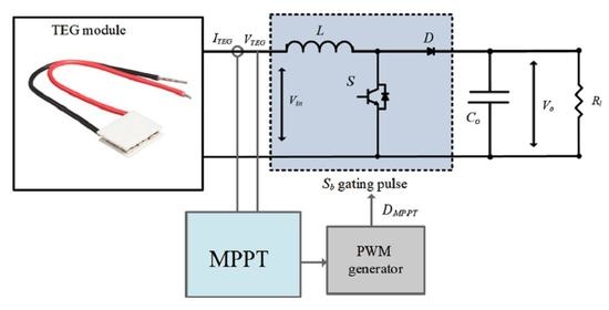
3.1. TEG Model

The structure of the TEG unit is presented in Figure 3a. The basic component of the TEG consists of a thermocouple containing the semiconductors from the types, as illustrated in Figure 3b,c. However, the TEG module can be created considering the number of “p” and “n” types of sets that are connected thermally in parallel to enhance the voltage and power outputs, and simultaneously to decrease the thermal resistance [5,10]. The couples are implanted among two parallel ceramic plates to develop hot and cold sides, as illustrated by Figure 3b. With applying a temperature difference within both hot and cold sides, a DC current will flow in the load.
Figure 4 shows the TEG system’s equivalent circuit, where the voltage open circuit, a source (VO.C), stands connected in series via an internal resistance (Rint); they are related to the load resistance (RL) [5,10]. In addition, the (Vteg) is the output voltage of the TEG module, applied on (RL).
The VO.C and Rint can be changed based on the temperature difference (ΔT) change of the hot-side temperature (Thot) and cold-side temperature (Tcold). The generated VOC can be formulated as:
V O . C = α s b × ( T h o t T c o l d ) = α s b × Δ T
where αsb is the Seebeck coefficient.
The αsb describes the induced TEG voltage (Vteg) in response to the ΔT within the material, as induced by the Seebeck effect. The thermoelectric component is a collection of a small series of “Piltier-junctions” that produce/absorb the heat once the current passes across it with a temperature gradient, called the “Thomson effect” [2].
According to the heat-energy equilibrium concept [38], the heat outflow of the heat energy flows from the high-temperature side (Qh) to the low-temperature side (Qc) and it is introduced by the following formula:
Q h = α s b I t e g T h o t + K Δ T 0.5 I t e g 2 R int
Q c = α s b I t e g T c o l d + K Δ T + 0.5 I t e g 2 R int
where K is the thermal conductivity coefficient. However, the output power Pteg of the TEG module is evaluated depending on the heat energy difference by the following equation:
P t e g = Q h Q c = ( α s b . Δ T I t e g R int ) I t e g = V t e g I t e g
Based on the circuit theory from Figure 4, the Vteg can be described as follows:
V t e g = α s b × Δ T I t e g R int = V O . C I t e g R int = I t e g R L
From Equations (8) and (9), the generated power of TEG system Pteg is able to be reformulated as follows:
P t e g = ( α s b × Δ T ) 2 R L ( R L + R int ) 2
In this work, the commercial datasheet of the TEG system is considered to be (TEG1–12611–6.0) [39].

3.2. Improved Fractional MPPT

The drawback of INR is the slow dynamic of tracking, whereas the drawback of P&O is the high oscillation around the MPP under steady-state conditions. Therefore, a fraction order-based MPPT has been proposed to overcome these drawbacks. Fraction control has been promoted in order to enhance the dynamic behavior of the traditional INR technique. The IFMPPT used a fractional PI instead of an integer integrator, which is illustrated by Figure 5. Fractional control contains a non-integer order, which provides more advantages, such as elasticity in construction and high forcefulness. However, the following Equation (11) defines the fractional PI transfer function [36]:
T c ( s ) = k p + k I s λ
where Tc symbolises the transfer function, k I   and   k p denote the integral and proportional constants, and λ denotes the fractional order.

4. Recent Optimization Algorithms

4.1. Moth-Flame Optimizer

Mirjalili et al. prepared the meta-heuristic optimizer named moth-flame optimization (MFO) [40]. MFO terminology is created based on the concept of moths’ transverse orientation that assigns a mechanization navigation in the dark. These insects (moths) take wing on a constant angle towards the moonlight’s location. The direction of moths will be in a direct line in a case where the source of light’s “flames” are far away. In the case of closed non-uniform flames/lights, the moths take a special direction, to exploit the global minimum solutions [40]. The MFO flowchart can be illustrated by Figure 6.
MFO is categorized as a population-based technique that sets as “M” matrix of moths based on the “n” number of moths ϵ [1, ..., n] and “d” search-space size ϵ [1, ..., d]. Hence, the objective functions of moths “OM” can be sorted in OM matrix ϵ [1, ..., n], which can generate the optimal solutions. In a similar manner to moths, the flames “F” can be evaluated. The step process of the MFO technique is implemented based on initialization function “I”, three approximation function, population function “P”, and the terminated criteria “T”.
The “I” function generates random moth population “rand” values of their corresponding objective functions, taking into account the upper “ub” and lower “lb” limits. These functions can be expressed as follows:
M ( i , j ) = ( u b ( i ) l b ( i ) ) r a n d ( n , d ) + l b ( i )
O M = F i t n e s s F u n c t i o n ( M )
Hence, the “P” function is initiated after the end of “I”, and it can be finished when the “T” criteria is performed. The “P” function leads the moths all over the place of the search space. The logarithmic spiral function is deemed to be the basic updating mechanism of each moth location with regards to the flame.
This location regarding a flame is renewed by the following expression:
M i = H ( M i , F j )
The logarithmic helix for the MFO optimizer is formed by the following expression:
H ( M i , F j ) = D I i e b t c o s ( 2 π t ) + F j
In this regard, the M i refers to the “ith-moth” and the F j is the “jth-flame”. The H is the helix-function. DIi defines the distance of the “ith-moth” and the “jth-flame”. “b” and “t” are defined as constant and random values, correspondingly.
Therefore, the DIi is evaluated by (16):
D I i = | F j M i |
Exploration happens once the following position determines the space frame between the moth and the flame. Alternatively, the exploitation is achieved by locating the next position inside the space frame amid moth and flame. Equation (17) illustrates that the flames’ number (Fno) gradually minimizes, regarding the iterations, to make certain the balance between the exploration and exploitation. Hence, the locations of the moths can be renewed in regards to the best flame at the end of iterations.
F   n o = r o u n d ( N f t i × N f 1 T m )
where Nf is the flames max number at the iteration “ti”. Tm is the max iteration number.
As mentioned above, the “P” function can be performed once the “T” function is terminated. Hence, the best moth can be returned, which is represented as the best developed rough calculation of the optimal.
In this paper, the duty cycle “D” of the DC-DC converter is deemed as one variable that represented as the moths’ value.

4.2. Particle Swarm Optimizer (PSO)

The PSO has been created considering the social thinking of a flock of birds [41]. It utilizes numerous particles as a global solution, which are employed through the search space for exploring the critical solution. To transfer/update the positioning of each particle, the present velocity, positioning, and pbest/gbest space should be determined. The valuation process of the PSO algorithm can be estimated based on the following equations. [41]:
ν i t 1 + t i = w * ν i t t i + c 1 * r 1 [ p b e s t i t t i x i t t i ] + c 2 * r 2 [ g b e s t i t t i x i t t i ]
x i t 1 + t i = x i t t i + Δ t * ν i t t i + 1
where ν i t t i introduces the velocity of particle “it”, “ti” is the No. of iterations under the random value “r1” and “r2” from 0 to 1, and “c1” and “c2” are constants to estimate the acceleration for the possible changes of particle rapidity considering the pbest and gbest directions. The positions can be modernized regarding Equation (19), wherever ∆t = 1.
However, during a series of iterations, the following equation was used to update the design parameter of an inertia factor w of the PSO technique:
w   t i + 1 = w   m a x ( w   m a x w   m i n ) t i / t i m a x
A time-varying inertia factor is typically set to 0.9 or 0.4, with wmax and wmin indicating its maximum and minimum values.
The performance characteristics of PSO, such as exploration capability, confidence, and the particles’ incorporation, can be estimated based on the Equation (18) [41]. The step process of the PSO technique is divided into the velocities’ evaluation depending upon Equation (18) and the updated positioning by Equation (19). The process can be stopped until the realizing of the optimal solutions.

4.3. Genetic Algorithm (GA)

The GA, created by Holland [42], can be considered as a kind of optimizer search methodology based on natural evolution and the theory of genetics. A population of individual solutions is repeatedly modified by the genetic algorithm. During each step, the genetic algorithm selects individuals from the current population to be parents and uses them to produce children for the coming generation. As generations progress, the population evolves toward an optimal solution. However, an optimization process was carried out in five stages, each involving a number of parameters that had to be considered. An overview of each stage of the process includes initialization, fitness function, selection, crossover, and mutation.
The coding process of GA can be performed based on a strain of finite length A = a1, a2, · · ·, aL, and AX = (x1, x2, · · ·, xn)T that is converted into a coded form of X, which can be noted as e(X). On the other hand, the X is named the decoding of A that can be noted by X = e −1 (A). The ai is deemed to be a gene. The amount of ai can be defined as binary rate/No. of floating points at L length. As a consequence, the HL = {A = a1, a2, · · ·, aL|ai ∈ Γ, i = 1, 2, · · ·, L} is relegated as separable space. In this case, the Hp is the number of dissimilar individuals. For the optimization issue, it is indispensable to look for the Hp and to estimate the fitness of the individual in Hp; thus, “A” fulfills maxAHp (A). In the tuple GAF(e, J, S, E, Ψ), its parameters are known as the coding layout, fitness metric, election and genetic operators, and parameter set. Hence, the GA operation can be determined by the following process:
(I)
Initialization. Produce the N individuals in the random form of the “initial population”, setting the evolution number.
(II)
Individual estimation. Estimate the fitness of every parameter according to the estimated criteria.
(III)
Population evolution. Perform the election, crossover, and mutation operations to deduce the step generation.
(IV)
Terminus check. If the fitness or iterations achieve their maximum solutions, stop the estimation process at that time; otherwise, return to (II).

4.4. Seagull Optimization Algorithm (SOA)

G. Dhiman and V. Kumar V [43] suggested a new type of bio-inspired optimization algorithm, named seagull optimizer, by analyzing the biological characteristics of seagulls. Seagulls live in groups, using their cleverness to detect and assault their prey. It is important to note that, in addition to their aggressive behavior, the most significant feature of seagulls is migration. During the migration operations, seagulls proceed from one position to another in order to meet three conditions:
I. 
Avoid collision: variable A is employed to evaluate the innovative positioning of the seagull’s search, in order to avoid collisions with other searches:
C s ( t ) = A × P s ( t )
A = f c ( t × ( f c / T max ) )
where Cs(t) represents a new position, which it is not entering a struggle with other search seagulls. The Ps(t) represents the position of the search seagull at the current iteration “t”. The motion manner, named “A”, is the variable of the search seagull in a given search area. fc can control the frequency of the adjustable, and its rate drops between 2 and 0.
II. 
Best position: After avoiding overlapping via other seagulls, seagulls can transfer in the direction of the innovative positioning:
M s ( t ) = B × ( P b s ( t ) P s ( t ) )
B = 2 × A 2 × r d
where Ms(t) represents the positions of the search seagull. The random number called “B” is responsible for balancing the global and local search seagull. rd is a random No. from 0 to 1.
III. 
Near the best search seagull: After the seagull moves into a position where it does not struggle with others, it moves into the best position in order to achieve its new position:
D s ( t ) = | C s ( t ) + M s ( t ) |
where, Ds(t) represents the best fit for the search seagull.
Seagulls have the capability to constantly exchange their attack angle and speed throughout their migration, depending on their wings/weight to keep themselves flying as high as possible. When attacking prey, they move in a helix shape in the air. The motion manner in the x, y, and z planes may be deduced by:
x = r × cos ( θ )
y = r × sin ( θ )
z = r × θ
r = u × e θ ν
where r is the helix radius at the random angle θ ϵ [0, 2π]. u and v are the correlation constants of the helix shape and e is the base of the natural logarithm. The attack position of seagulls is constantly updated:
P s ( t ) = D s ( t ) × x × y × z + P b s ( t )
where Ps(t) maintains the best solution and modernizes the positioning of other search seagulls.

4.5. Grey Wolf Optimization (GWO)

The GWO algorithm has been developed as an optimization method to simulate the leadership hierarchy and hunting strategy of gray wolves [44]. Four levels of leadership hierarchy exist in the gray wolf flock: alpha (α), beta (β), delta (δ), and omega (ω). The alpha wolf, which is at the top of the gray wolf hierarchy, oversees the entire pack. In the hierarchy, alpha is at the top and beta is at the bottom; they help the alpha make decisions and control everything else. The following wolves dominate the omega level of the hierarchy: leaders such as alpha are in charge of the hunting process, followed by betas and deltas. GWO uses an alpha analogy to determine the best fitness solution. Beta represents the second-best solution, delta represents the third-best, and omega represents the remaining solutions [44].
Mathematically, it is assumed that beta, alpha, and delta wolves have a good knowledge of the possible positions of prey and that omega wolves update its location based on their knowledge. Therefore, the following formula can be very applicable:
D α = | C 1 . X α X i ( t ) | , D β = | C 2 . X β X i ( t ) | , D δ = | C 3 . X δ X i ( t ) |
X 1 = | X α A 1 . D α | , X 2 = | X β A 2 . D β | , X 3 = | X δ A 3 . D δ |
X i G W O ( t + 1 ) = X 1 + X 2 + X 3 3
where X and D introduce the location and coefficient vectors of (α), (β), and (δ) wolves at iteration t. In the following iteration, the location vector X i G W O ( t + 1 ) can be introduced at the ith grey wolf. The other coefficient vectors A and C can be acknowledged by the following formula:
A = 2 a r 1 a C = 2 r 2
where the random vectors r1 and r2 are ϵ [0, 1]. The factor a can be decreased from 2 to 0 throughout the iteration process, and it can be formulated as follows:
a = 2 ( 1 t T )

4.6. Tunicate Swarm Algorithm

The TSA is a metaheuristic optimizer inspired by the work of S. Kaur et al. [45]. The TSA emulates the swarming positions of marine tunicates and their jet propulsions as they navigate and search for food. During the process of the TSA, the TSA population (TP) swarms as they seek the most suitable source of food (SF), which can be introduced as the fitness function. Based on the swarming operation, the updated positions of tunicates are entered regarding the first finest tunicates, which are put in storage with upgrades in each iteration. Therefore, the operation of TSA is started by initializing the random population of tunicates, taking into account the control variables’ boundaries. The control variables’ dimension “Dim” can represent each tunicate (T), deduced by the following formula:
T n ( m ) = T n min + r . ( T n max T n min ) , m T P s i z e , n D i m
where T(m) is the positioning of every tunicate (m) considering the random No. r ϵ [0, 1]. n denotes every managed variable.
The update procedure of the TP is performed based on (35):
T n ( m ) = T n * ( m ) + T n ( m 1 ) 2 + c 1
where T* denotes the updated position of the mth tunicate, T(m − 1) denotes the neighbor tunicate according to (36), and c1 is a random No. from 0 to 1.
T n * ( m ) = { S F + A t . | S F r a n d . T n ( m ) | i f   r a n d 0.5 S F A t . | S F r a n d . T n ( m ) | i f   r a n d < 0.5
where SF is denoted by the best TP.
At is a randomized vector that avoids the possible disputes among tunicates. The At is formulated as follows:
A t = c 2 + c 3 2 c 1 V T min + c 1 ( V T max V T min )
where c1, c2, and c3 are random ϵ [0, 1]. VTmin and VTmax represent the first and subordinate speeds to deduce the social interaction.

5. Results and Discussion

In this work, the TEG (TEG1–12611–6.0) is adopted and its specifications can be found in [38]. IFMPPT parameters’ estimation are performed using six optimization methodologies, including MFO, PSO, GA, SOA, GWO, and TSA. The total energy of the TEG is implemented as the objective function that needs to be maximized during the optimization procedure while three parameters are applied as decision variables: integration gain, proportional gain, and fraction order. In order to make the comprehensive analysis fair, the population size and the maximum iteration number for the applied methodologies have set values of 10 and 25. The best parameters of optimized fractional MPPTS applying different optimizers are presented in Table 1. To confirm the consistency of the applied algorithms, every optimization ran 30 times. The numerical evaluations of the applied techniques are illustrated by Table 2.
Based on Table 1, the mean objective function values ranged from 1.01886 to 1.35336. The highest one is accomplished by MFO. The STD values ranged from 0.01968 to 0.32809. The lowest STD was also accomplished by MFO. Regarding the efficiency, the maximum efficiency of 98.31% was achieved by MFO while the lowermost efficiency of 72.49 % was reached by TSA. The details of 30 runs are presented in Table 2 and Figure 7.
On the other hand, an analysis of the variance test (ANOVA) has been performed to verify the consistency of the prepared MFO in solving the design problematic. Table 3 approves the variance of the performance provided by each algorithm. The graphic results in Figure 8 present the variation ratio of each optimizer; this figure demonstrates that the lowest variation with best fitness can be provided by the MFO algorithm.
In this study, the performance of a fractional MPPT based upon the MFO optimizer is analyzed with regards to the temperature change as well as the load change after the optimum parameters have been defined. The intention is to change the operational condition in order to assess how the suggested strategy performs under dynamic stalking conditions. The TEG power system contains one TEG module, enhancing the converter’s performance in unbroken direct current mode with an interchanging frequency of 30 kHz, an input inductance of 1 mH, and an output capacitor of 47 F with 10 Ω load value. In a time of 0.6 s, an additional resistance of 10 Ω is added in parallel with the load. The temperature of the cold side of the TEG decreased from 50 °C to 30 °C in 0.25 s, and then reached 50 °C in 0.8 s. Meanwhile, the hot-side temperature rises from 250 °C to 300 °C in 0.25 s, and then returns to 250 °C in 0.8 s. Table 4 shows the different scenarios considered.
To reveal the prevalence of the MFO based upon MPPT, the comprehensive analysis of the tracking performance has been carried out via standard INR and P&O methods. For the standard INR methodology, it has been supposed that the gain of the discrete integrator is 0.8. On the other hand, with MFO-based MPPT, the IFMPPT parameters are 0.03484, 6.74872, and 0.97195, respectively, for proportional gain, integral gain, and fractional order, as outlined applying MFO, and shown in Table 1.
Figure 9a demonstrates the TEG power for three MPPTs with altering operational conditions. Notably, the MFO-based MPPT reaches the maximum power of 9.4 W very fast compared INR and P&O. The INR needs extra time to reach to the MPP because of its slow dynamic. The fluctuations around the MPP are eliminated through MFO-based MPPT compared with P&O. At the time of 0.6 s, the load worth is reduced from 10 Ω to 5 Ω. The MFO-based MPPT generally returns to MPP quickly. However, the normal strategies need longer to regulate the duty cycle to urge MPP. Additionally, at the time of 0.8 s, the temperature distinction is diminished from 270 to 200 °C. The following performance of the MFO-based MPPT is the most typical one. The whole variation of TEG current and voltage, in addition to the duty cycle, can be illustrated by Figure 9b–d, respectively.

6. Conclusions

An optimized fractional MPPT methodology has been prepared to obtain the most out of the harvested energy from a thermoelectric generator system. The best parameters of the optimized fractional tracker were determined using MFO. To prove the pre-eminence of MFO, the comprehensive analysis of the existing results was performed via PSO, genetic algorithm, grey wolf optimization, seagull optimization algorithm, and tunicate swarm algorithm. The mean objective function values ranged from 1.01886 to 1.35336. The highest one was accomplished by MFO. The STD values ranged from 0.01968 to 0.32809. The least standard value was also accomplished by MFO. Regarding the efficiency, the highest value of 98.31% was obtained by MFO, but the smallest one of 72.49% was obtained by TSA. In sum, the improved fractional MPPT succeeded in boosting the dynamic response and diminishing the steady-state fluctuations compared with conventional MPPT methods. Overall, the fractional MPPT that was a step forward succeeded in reinforcing the dynamic reaction and lessening the steady-state fluctuations in comparison to traditional MPPT methods. Finally, reducing the number of required sensors will be considered in future work.

Author Contributions

All the authors have contributed to this research. Conceptualization, H.R. and M.A.T.; methodology, H.R. and M.A.T.; software, H.R. and M.A.; validation, H.R., M.M.Z. and M.A.T.; formal analysis, M.A.T.; investigation, M.A. and M.M.Z.; resources, H.R. and M.M.Z.; data curation, M.A. and M.M.Z.; writing—original draft preparation, H.R. and M.A.T.; writing—review and editing, H.R. and M.A.T.; visualization, M.A. and M.M.Z.; supervision, H.R. and M.M.Z.; project administration, H.R. and M.A.T.; funding acquisition, H.R. and M.A.T. All authors have read and agreed to the published version of the manuscript.

Funding

This research received no external funding.

Data Availability Statement

Not applicable.

Conflicts of Interest

The authors declare no conflict of interest or non-financial competing interest.

References

  1. Olabi, A.G. 100% sustainable energy. Energy 2014, 77, 1–5. [Google Scholar] [CrossRef]
  2. Olabi, A.; Abdelkareem, M. Energy storage systems towards 2050. Energy 2020, 219, 119634. [Google Scholar] [CrossRef]
  3. Bucolo, M.; Buscarino, A.; Famoso, C.; Fortuna, L.; Gagliano, S. Imperfections in Integrated Devices Allow the Emergence of Unexpected Strange Attractors in Electronic Circuits. IEEE Access 2021, 9, 29573–29583. [Google Scholar] [CrossRef]
  4. Akram, N.; Khan, L.; Agha, S.; Hafeez, K. Global Maximum Power Point Tracking of Partially Shaded PV System Using Advanced Optimization Techniques. Energies 2022, 15, 4055. [Google Scholar] [CrossRef]
  5. Rezk, H.; Ali, Z.M.; Abdalla, O.; Younis, O.; Gomaa, M.R.; Hashim, M. Hybrid Moth-Flame Optimization Algorithm and Incremental Conductance for Tracking Maximum Power of Solar PV/Thermoelectric System under Different Conditions. Mathematics 2019, 7, 875. [Google Scholar] [CrossRef] [Green Version]
  6. Olabi, A. State of the art on renewable and sustainable energy. Energy 2013, 61, 2–5. [Google Scholar] [CrossRef]
  7. Atems, B.; Hotaling, C. The effect of renewable and nonrenewable electricity generation on economic growth. Energy Policy 2018, 112, 111–118. [Google Scholar] [CrossRef]
  8. Olabi, A.; Abdelkareem, M.A. Renewable energy and climate change. Renew. Sustain. Energy Rev. 2022, 158, 112111. [Google Scholar] [CrossRef]
  9. Ando Junior, O.H.; Maran, A.L.O.; Henao, N.C. A review of the development and applications of thermoelectric microgenerators for energy harvesting. Renew. Sustain. Energy Rev. 2018, 91, 376–393. [Google Scholar] [CrossRef]
  10. Twaha, S.; Zhu, J.; Yan, Y.; Li, B.; Huang, K. Performance analysis of thermoelectric generator using dc-dc converter with incremental conductance based maximum power point tracking. Energy Sustain. Dev. 2017, 37, 86–98. [Google Scholar] [CrossRef]
  11. Yang, B.; Zhang, M.; Zhang, X.; Wang, J.; Shu, H.; Li, S.; He, T.; Yang, L.; Yu, T. Fast atom search optimization based MPPT design of centralized thermoelectric generation system under heterogeneous temperature difference. J. Clean. Prod. 2019, 248, 119301. [Google Scholar] [CrossRef]
  12. Zheng, X.; Liu, C.; Yan, Y.; Wang, Q. A review of thermoelectrics research – Recent developments and potentials for sustainable and renewable energy applications. Renew. Sustain. Energy Rev. 2014, 32, 486–503. [Google Scholar] [CrossRef]
  13. Mojtaba, M.; Alireza, R.; Lasse, R. Power optimization and economic evaluation of thermoelectric waste heat recovery system around a rotary cement kiln. J. Clean. Prod. 2019, 232, 1321–1334. [Google Scholar]
  14. Matthew, B.; Jae, D.P. Current-sensorless power estimation and MPPT implementation for thermoelectric generators. IEEE Trans. Indust. Elect. 2015, 62, 5539–5548. [Google Scholar]
  15. Gou, X.; Xiao, H.; Yang, S. Modeling, experimental study and optimization on low-temperature waste heat thermoelectric generator system. Appl. Energy 2010, 87, 3131–3136. [Google Scholar] [CrossRef]
  16. Rowe, D. Thermoelectrics, an environmentally-friendly source of electrical power. Renew. Energy 1999, 16, 1251–1256. [Google Scholar] [CrossRef]
  17. Liang, G.; Zhou, J.; Huang, X. Analytical model of parallel thermoelectric generator. Appl. Energy 2011, 88, 5193–5199. [Google Scholar] [CrossRef]
  18. Chen, M.; Rosendahl, L.; Condra, T. A three-dimensional numerical model of thermoelectric generators in fluid power systems. Int. J. Heat Mass Transf. 2010, 54, 345–355. [Google Scholar] [CrossRef]
  19. Kramer, L.R.; Maran, A.L.O.; de Souza, S.S.; Junior, O.H.A. Analytical and Numerical Study for the Determination of a Thermoelectric Generator’s Internal Resistance. Energies 2019, 12, 3053. [Google Scholar] [CrossRef] [Green Version]
  20. Kim, S. Analysis and modeling of effective temperature differences and electrical parameters of thermoelectric generators. Appl. Energy 2013, 102, 1458–1463. [Google Scholar] [CrossRef]
  21. Ding, L.; Akbarzadeh, A.; Tan, L. A review of power generation with thermoelectric system and its alternative with solar ponds. Renew. Sustain. Energy Rev. 2018, 81, 799–812. [Google Scholar] [CrossRef]
  22. Zhao, Y.; Wang, S.; Ge, M.; Li, Y.; Liang, Z. Analysis of thermoelectric generation characteristics of flue gas waste heat from natural gas boiler. Energy Convers. Manag. 2017, 148, 820–829. [Google Scholar] [CrossRef]
  23. Montecucco, A.; Siviter, J.; Knox, A. Combined heat and power system for stoves with thermoelectric generators. Appl. Energy 2017, 185, 1336–1342. [Google Scholar] [CrossRef] [Green Version]
  24. Moh’d, A.A.; Ahmed, A.A. Internal combustion engine waste heat recovery by a thermoelectric generator inserted at combustion chamber walls. Intern. J. Energ. Res. 2018, 42, 4853–4865. [Google Scholar]
  25. Cao, Q.; Luan, W.; Wang, T. Performance enhancement of heat pipes assisted thermoelectric generator for automobile exhaust heat recovery. Appl. Therm. Eng. 2018, 130, 1472–1479. [Google Scholar] [CrossRef]
  26. Ioan, S.; Alexandru, D. A comprehensive review of solar thermoelectric cooling systems. Int. J. Energy Res. 2018, 42, 395–415. [Google Scholar]
  27. Li, L.; Gao, X.; Zhang, G.; Xie, W.; Wang, F.; Yao, W. Combined solar concentration and carbon nanotube absorber for high performance solar thermoelectric generators. Energy Convers. Manag. 2019, 183, 109–115. [Google Scholar] [CrossRef]
  28. Kashif, I.; Khairul, H.; Saidur, R.; Kareem, M.W.; Bidyut, B.S. Study of thermoelectric and photovoltaic facade system for energy efficient building development: A review. J. Clean. Prod. 2019, 209, 1376–1395. [Google Scholar]
  29. Khatua, S.; Mukherjee, V. Application of integrated microgrid for strengthening the station blackout power supply in nuclear power plant. Prog. Nucl. Energy 2019, 118, 103132. [Google Scholar] [CrossRef]
  30. Kanagaraj, N. An Enhanced Maximum Power Point Tracking Method for Thermoelectric Generator Using Adaptive Neuro-Fuzzy Inference System. J. Electr. Eng. Technol. 2021, 16, 1207–1218. [Google Scholar] [CrossRef]
  31. Tang, Z.B.; Deng, Y.D.; Su, C.Q.; Shuai, W.W.; Xie, C.J. A research on thermoelectric generator’s electrical performance under temperature mismatch conditions for automotive waste heat recovery system. Case Stud. Therm. Eng. 2015, 5, 143–150. [Google Scholar] [CrossRef] [Green Version]
  32. Zhang, Z.; Zhang, Y.; Sui, X.; Li, W.; Xu, D. Performance of Thermoelectric Power-Generation System for Sufficient Recovery and Reuse of Heat Accumulated at Cold Side of TEG with Water-Cooling Energy Exchange Circuit. Energies 2020, 13, 5542. [Google Scholar] [CrossRef]
  33. Derbeli, M.; Barambones, O.; Sbita, L. A Robust Maximum Power Point Tracking Control Method for a PEM Fuel Cell Power System. Appl. Sci. 2018, 8, 2449. [Google Scholar] [CrossRef] [Green Version]
  34. Fathy, A.; Abdelkareem, M.A.; Olabi, A.; Rezk, H. A novel strategy based on salp swarm algorithm for extracting the maximum power of proton exchange membrane fuel cell. Int. J. Hydrogen Energy 2020, 46, 6087–6099. [Google Scholar] [CrossRef]
  35. Montecucco, A.; Knox, A.R. Maximum Power Point Tracking Converter Based on the Open-Circuit Voltage Method for Thermoelectric Generators. IEEE Trans. Power Electron. 2014, 30, 828–839. [Google Scholar] [CrossRef]
  36. Al-Dhaifallaha, M.; Nassefa, A.M.; Rezk, H.; Nisar, K.S. Maximum Power Point Tracking Converter Based on the Open-Circuit Voltage Method for Thermoelectric Generators. Solar Energy 2018, 159, 650–664. [Google Scholar]
  37. Taghvaee, M.; Radzi, M.A.M.; Moosavain, S.; Hizam, H.; Marhaban, M.H. A current and future study on non-isolated DC–DC converters for photovoltaic applications. Renew. Sustain. Energy Rev. 2012, 17, 216–227. [Google Scholar] [CrossRef]
  38. Shanmugam, S.; Eswaramoorthy, M.; Veerappan, A.R. Modeling and Analysis of a Solar Parabolic Dish Thermoelectric Generator. Energy Sources Part A Recover. Util. Environ. Eff. 2014, 36, 1531–1539. [Google Scholar] [CrossRef]
  39. Datasheet “TEG1-12611-6.0”. Available online: https://thermoelectric-generator.com/product/teg1-12611-6-0/.pdf (accessed on 29 April 2022).
  40. Tolba, M.A.; Diab, A.A.Z.; Tulsky, V.N.; Abdelaziz, A.Y. LVCI approach for optimal allocation of distributed generations and capacitor banks in distribution grids based on moth–flame optimization algorithm. Electr. Eng. 2018, 100, 2059–2084. [Google Scholar] [CrossRef]
  41. Kennedy, J.; Eberhart, R.C. Particle swarm optimization. In Proceedings of the IEEE International Conference on Neural Networks IV, Perth, WA, Australia, 27 November–1 December 1995; IEEE Service Center: Piscataway, NJ, USA, 1995; pp. 1942–1948. [Google Scholar]
  42. Holland, J.H. Adaptation in Natural and Artificial Systems: An introductory analysis with applications to biology, Control, and Artificial Intelligence; University of Michigan Press: Ann Arbor, MI, USA, 1975; pp. 126–137. [Google Scholar]
  43. Dhiman, G.; Kumar, V. Seagull optimization algorithm: Theory and its applications for large-scale industrial engineering problems. Knowledge-Based Syst. 2018, 165, 169–196. [Google Scholar] [CrossRef]
  44. Mirjalili, S.; Mirjalili, S.M.; Lewis, A. Grey Wolf Optimizer. Adv. Eng. Softw. 2014, 69, 46–61. [Google Scholar] [CrossRef] [Green Version]
  45. Kaur, S.; Awasthi, L.K.; Sangal, A.; Dhiman, G. Tunicate Swarm Algorithm: A new bio-inspired based metaheuristic paradigm for global optimization. Eng. Appl. Artif. Intell. 2020, 90, 103541. [Google Scholar] [CrossRef]
Figure 1. Flowchart of conventional P&O methodology.
Energies 15 08836 g001
Figure 2. Flowchart of conventional INR method.
Energies 15 08836 g002
Figure 3. Construction of the TEG.
Energies 15 08836 g003
Figure 4. The sample circuit of the TEG component.
Energies 15 08836 g004
Figure 5. MATLAB model of optimized fractional MPPTS.
Energies 15 08836 g005
Figure 6. The evaluation process of MFO.
Energies 15 08836 g006
Figure 7. Details of 30 runs applying the studied algorithms.
Energies 15 08836 g007
Figure 8. ANOVA test results.
Energies 15 08836 g008
Figure 9. Detailed tracking performance using different MPPTs. (a) TEG power, (b) TEG current, (c) TEG voltage, and (d) duty cycle.
Energies 15 08836 g009aEnergies 15 08836 g009b
Table 1. Best parameters of IFMPPT and numerical evaluation (30 runs).
ParameterPSOGAGWOSOATSAMFO
Kp0.033460.03320.037650.0010.035170.03484
Ki6.67765.475988.434515.376086.804296.74872
λ0.984580.94251.010080.960990.983410.97195
Best1.37571.371311.376661.359831.376371.37654
Worst0.576940.578550.612780.613460.576941.32855
Average1.105991.018861.222651.270030.997961.35336
Median1.328880.986221.332791.326630.885281.36039
Variance0.101160.079060.071810.033790.107650.00039
STD0.318060.281170.267970.183810.328090.01968
Efficiency80.3474.0188.8192.2572.4998.31
Table 2. Details of 30 runs applying studied algorithms.
RunPSOGAGWOSOATSAMFO
10.72750.984870.665671.326921.348370.7275
21.326420.64940.729891.323391.331451.32642
31.366230.988961.376661.327880.798931.36623
41.327960.987571.376581.326920.952361.32796
51.363411.33411.330731.298971.330721.36341
60.781131.132021.328121.325941.376370.78113
71.37571.258711.329741.325671.36621.3757
81.339151.366771.34311.326950.818211.33915
91.367490.9540.61281.326350.998461.36749
101.333970.785811.329071.327960.602741.33397
110.712081.360861.376631.327120.729190.71208
121.329790.711631.375531.328130.576941.32979
130.576941.371311.329081.330371.372290.57694
141.331741.346471.37581.328410.607881.33174
150.791991.355410.96821.328861.376140.79199
161.361840.765591.329511.328530.749561.36184
170.600961.364791.329771.349260.657410.60096
181.341761.333241.334861.322781.376211.34176
190.685071.271441.329351.310731.330990.68507
201.372220.835861.376661.320820.730831.37222
211.312990.753341.336931.353160.729191.31299
220.704880.804831.329861.327640.576940.70488
231.372241.280261.375971.317121.372291.37224
241.344350.787671.376361.359830.607881.34435
250.683230.723891.375240.613461.376140.68323
261.350980.661111.364571.028360.749561.35098
270.612781.346720.612781.325380.657410.61278
281.360420.609551.376061.325621.376211.36042
290.736530.578551.371261.324871.330990.73653
301.288030.861160.612780.613460.730831.28803
Table 3. ANOVA numeric results.
SourceSSdfMSFp-Value > F
Columns3.07550.6159.061.13667 × 10−7
Error11.81451740.0679
Total14.8904179
Table 4. Different scenarios considered.
Time Period Hot-Side
Temperature
Cold-Side
Temperature
Load
Resistance
TEG Maximum PowerTEG Current at MPPTEG Voltage at MPP
0 s to 0.25 s250 °C50 °C10 Ω9.4 W2.88 A3.25 V
0.25 s to 0.6 s300 °C30 °C10 Ω14.6 W3.4 A4.2 V
0.6 s to 0.8 s300 °C30 °C5 Ω14.6 W3.4 A4.2 V
0.8 s to 1.0 s250 °C50 °C5 Ω9.4 W2.88 A3.25 V
Publisher’s Note: MDPI stays neutral with regard to jurisdictional claims in published maps and institutional affiliations.

