
Improvement of Gas Compressibility Factor and Bottom-Hole Pressure Calculation Method for HTHP Reservoirs: A Field Case in Junggar Basin, China


 and
and 
Abstract
1. Introduction
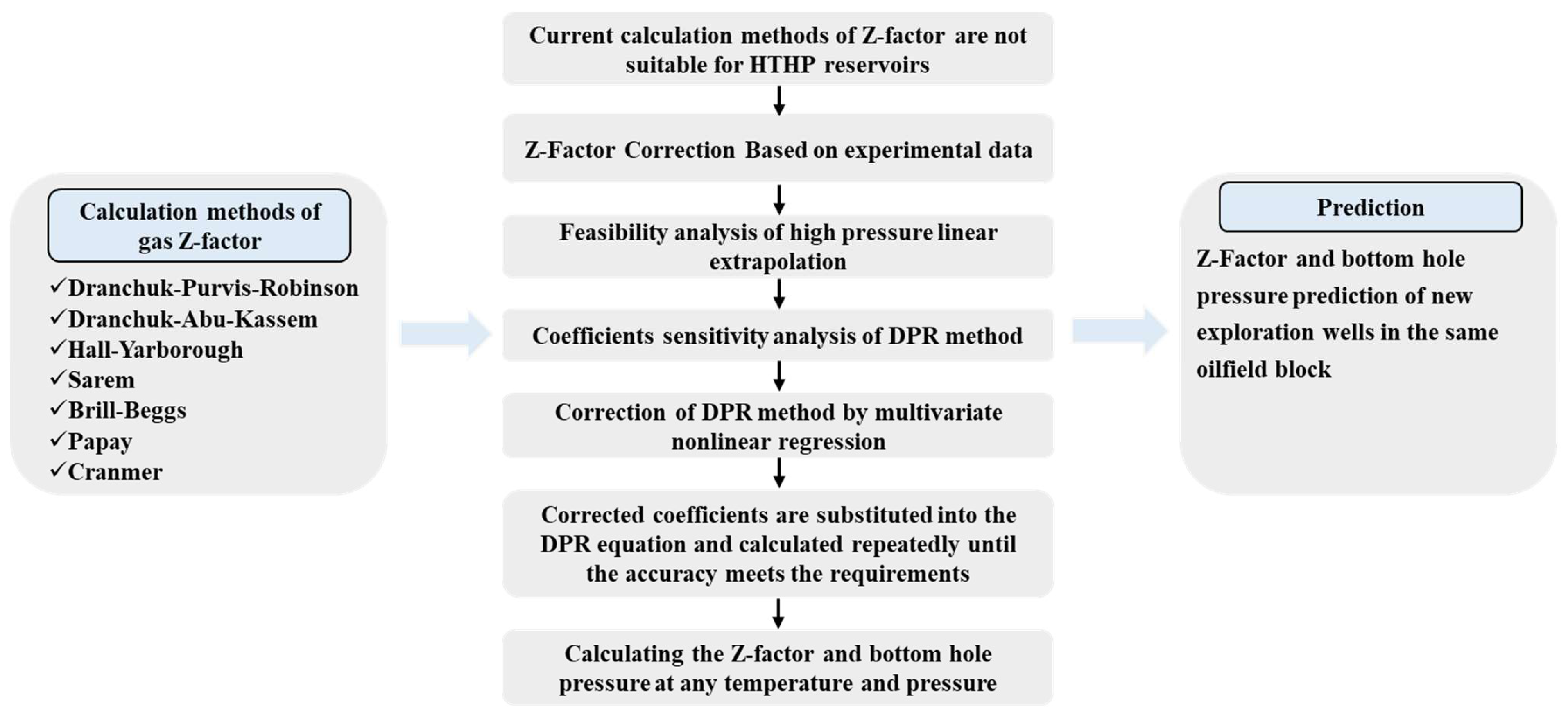
2. Methodology
2.1. Gas Z-Factor Correction
2.1.1. Feasibility Analysis of Linear Extrapolation
2.1.2. Error Analysis of Z-Factor Empirical Formula
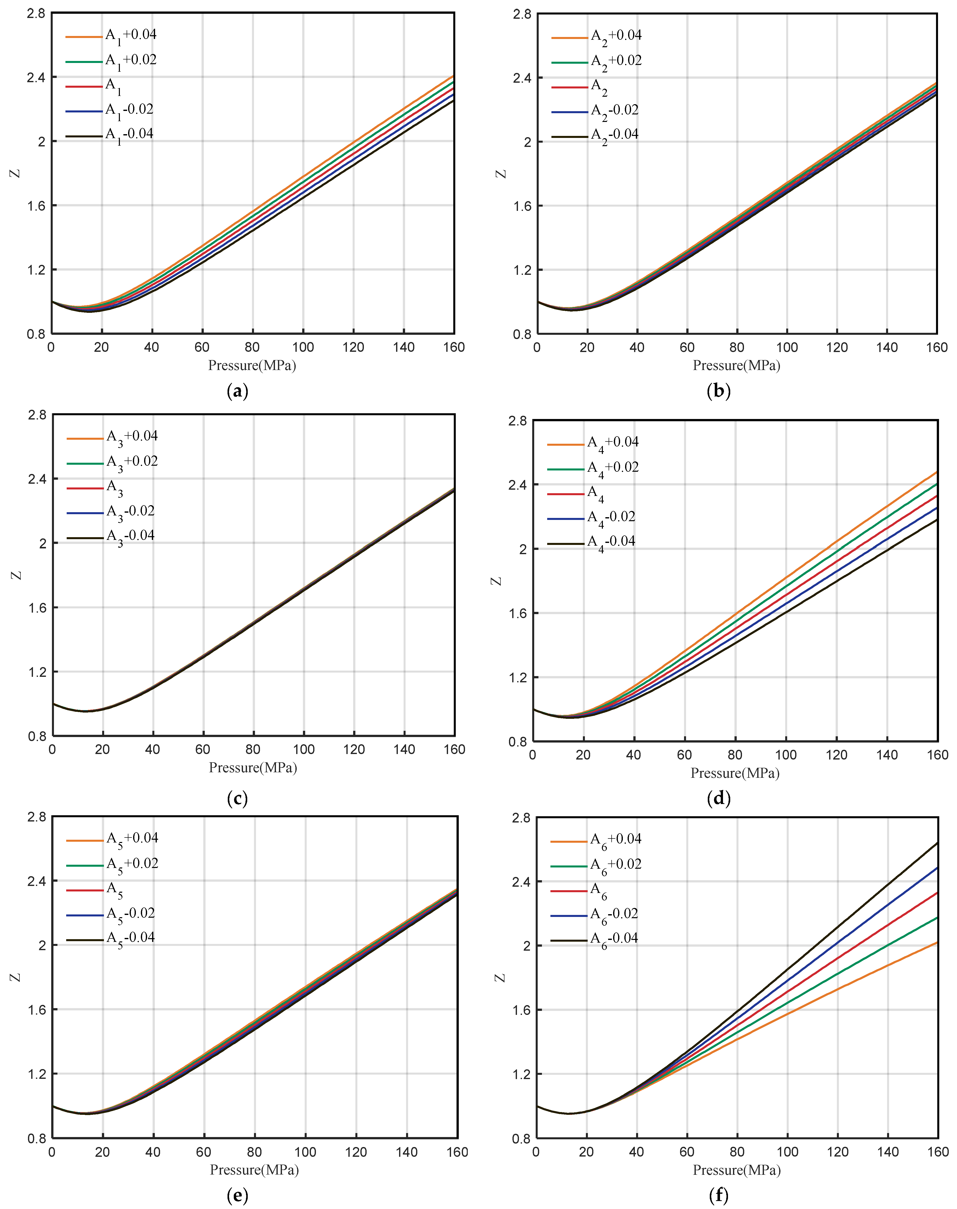
2.1.3. Coefficients Sensitivity Analysis of DPR Method
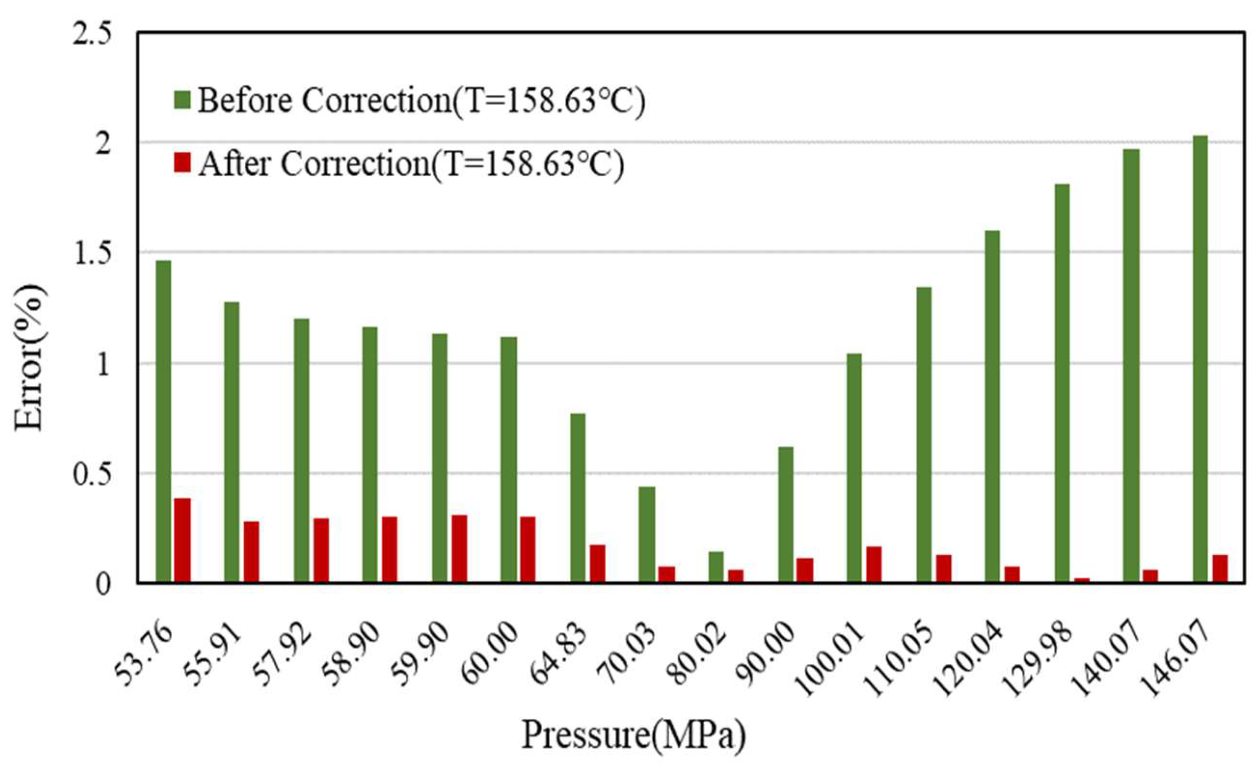
2.1.4. Correction of DPR Method by Multivariate Nonlinear Regression
2.2. PVT Parameter Calculation
2.3. Bottom Hole Pressure Calculation of Gas Well
- (1)
- According to the wellhead pressure and temperature conditions, the value of the subscript 1 numerical term in the denominator of Equation (18) is calculated. Assuming that the midpoint numerical term is equal to the subscript 1 numerical term, the initial value of the pressure in the middle of the wellbore is calculated;
- (2)
- According to the temperature in the middle of the wellbore and the above-calculated pressure value, the numerical value of the subscript m in the denominator of Equation (18) is calculated, and the pressure value in the middle of the wellbore is calculated again according to Equation (18);
- (3)
- Comparing the pressure difference between step (2) and the last calculation (the first step is the estimation), if the difference is large, step (2) iterative calculation is repeated until the calculation error meets the requirements;
- (4)
- After determining the pressure in the middle of the wellbore, the above steps are used to further iteratively calculate the bottom hole pressure.
3. Case Study and Prediction
3.1. Case 1
3.2. Case 2
4. Conclusions
- (1)
- The sensitivity analysis of DPR correlation shows that the coefficients A4 and A6 are sensitive to high pressure and satisfy the demand for correction. The new correlation can be used to determine the Z-factor at any pressure range, especially for high pressures, and the error is less than 1% compared to the PVT data;
- (2)
- The error between the natural gas density calculated by the corrected Z-factor and the PVT data is within 1%, and the error between the formation volume factor and the PVT data is within 0.5%. At the same time, the variation trend of the gas isothermal compressibility coefficient and gas viscosity of well H1 with pressure is predicted;
- (3)
- Under the condition of a formation depth of 7374 m, the bottom hole pressure calculated before and after the correction of the Z-factor is 143.58 MPa and 146.32 MPa, respectively. Compared with the actual measured value of 146.07 MPa, the corrected Z-factor is closer to the actual value;
- (4)
- It is predicted that the bottom hole pressure of well H2 is 171.84 MPa and the gas Z-factor is 2.3548 when the formation depth is 8079 m, and the Z-factor chart at different temperatures is provided.
Author Contributions
Funding
Institutional Review Board Statement
Informed Consent Statement
Data Availability Statement
Acknowledgments
Conflicts of Interest
Nomenclature
| Z | gas compressibility factor |
| Tpr | pseudo-reduced temperature |
| Ppr | pseudo-reduced pressure |
| P | intermolecular interaction (MPa) |
| PR | intermolecular repulsion (MPa) |
| PA | intermolecular attraction (MPa) |
| R | state equation constant |
| T | temperature (K) |
| V | Volume (m3) |
| a | empirical constants of VDW state equation |
| b | empirical constants of VDW state equation |
| Ppc | pseudo critical pressure (MPa) |
| Tpc | pseudo critical temperature (K) |
| pci | critical pressure of component i (MPa) |
| Tci | critical temperature of component i (K) |
| xi | mole fraction of component i |
| ρr | gas reduced density |
| ρg | gas density (g/cm3) |
| Ma | gas relative molecular weight |
| Bg | formation volume factor (m3/m3) |
| pwf | bottom hole pressure (MPa) |
| pwh | wellhead pressure (MPa) |
| D | tubing inner-diameter (m) |
| f | frictional coefficient |
| q | rate of the gas (m3/d) |
| γg | gas relative density |
| H | depth of tubing down to the middle of formation (m) |
| HTHP | high temperature and high pressure |
| DPR | Dranchuk, Purvis, and Robinson |
References
- Wang, Y.; Ayala, L.F. Explicit Determination of Reserves for Variable Bottom-hole Pressure Conditions in Gas Well Decline Analysis. SPE J. 2020, 25, 369–390. [Google Scholar] [CrossRef]
- Wei, C.; Liu, Y.; Deng, Y.; Cheng, S.; Hassanzadeh, H. Temperature Transient Analysis of Naturally Fractured Geothermal Reservoirs. SPE J. 2022, 27, 2723–2745. [Google Scholar] [CrossRef]
- Luo, L.; Cheng, S.Q.; Lee, J. Characterization of refracture orientation in poorly propped fractured wells by pressure transient analysis: Model, pitfall, and application. J. Nat. Gas Sci. Eng. 2020, 79, 1875–5100. [Google Scholar] [CrossRef]
- Mahmoud, M.A. Development of a New Correlation of Gas Compressibility Factor (Z-Factor) for High Pressure Gas Reservoir. In Proceedings of the North Africa Technical Conference and Exhibition, Cairo, Egypt, 15–17 April 2013. [Google Scholar] [CrossRef]
- Wang, Y.; Cheng, S.; Zhang, F.; Feng, N.; Li, L.; Shen, X.; Li, J.; Yu, H. Big Data Technique in the Reservoir Parameters’ Prediction and Productivity Evaluation: A Field Case in Western South China Sea. Gondwana Res. 2021, 96, 22–36. [Google Scholar] [CrossRef]
- Wei, C.; Liu, Y.; Deng, Y.; Cheng, S.; Hassanzadeh, H. Analytical well-test model for hydraulicly fractured wells with multiwell interference in double porosity gas reservoirs. J. Nat. Gas Sci. Eng. 2022, 103, 1875–5100. [Google Scholar] [CrossRef]
- Zhang, C.; Cheng, S.; Wang, Y.; Chen, G.; Yan, K.; Ma, Y. Rate Transient Behavior of Wells Intercepting Non-Uniform Fractures in a Layered Tight Gas Reservoir. Energies 2022, 15, 5705. [Google Scholar] [CrossRef]
- Abolghasemi, E.; Andersen, P.Ø. The influence of adsorption layer thickness and pore geometry on gas production from tight compressible shales. Adv. Geo-Energy Res. 2021, 6, 4–22. [Google Scholar] [CrossRef]
- Wei, Q.; Wang, Y.; Han, D.; Sun, M.; Huang, Q. Combined effects of permeability and fluid saturation on seismic wave dispersion and attenuation in partially-saturated sandstone. Adv. Geo-Energy Res. 2021, 5, 181–190. [Google Scholar] [CrossRef]
- Kumar, M.N. Compressibility Factors for Natural and Sour Reservoir Gases by Correlations & Cubic Equations of State; Texas Tech University: Lubbock, TX, USA, 2004; Available online: http://hdl.handle.net/2346/15386 (accessed on 6 September 2022).
- Ghanem, A.; Gouda, M.F.; Alharthy, R.D.; Desouky, S.M. Predicting the Compressibility Factor of Natural Gas by Using Statistical Modeling and Neural Network. Energies 2022, 15, 1807. [Google Scholar] [CrossRef]
- Jia, D.; Zhu, X.; Song, L.; Liang, X.; Li, L.; Li, H.; Li, Z. New Model of Granite Buried-Hill Reservoir in PL Oilfield, Bohai Sea, China. Energies 2022, 15, 5702. [Google Scholar] [CrossRef]
- Standing, M.B.; Katz, D.L. Density of Natural Gases. Trans. AIME 1942, 146, 140–149. [Google Scholar] [CrossRef]
- Yarborough, L.; Hall, K.R. A New Equation of State for Z-Factor Calculations. Oil Gas J. 1973, 71, 82–92. [Google Scholar]
- Yarborough, L.; Hall, K.R. How to Solve Equation of State for Z-Factors. Oil Gas J. 1974, 72, 86–88. [Google Scholar]
- Benedict, M.; Webb, G.B.; Rubin, L.C. An Empirical Equation of Thermodynamic Properties of Light Hydrocarbon and Their Mixtures, I. Methane, Ethane, Propane, and n-Butane. J. Chem. Phys. 1940, 8, 334–345. [Google Scholar] [CrossRef]
- Dranchuk, P.M.; Purvis, R.A.; Robinson, D.B. Computer Calculation of Natural Gas Compressibility Factors Using the Standing and Katz Correlation. In Proceedings of the Annual Technical Meeting, Edmonton, AB, Canada, 7–11 May 1973. [Google Scholar] [CrossRef]
- Dranchuk, P.M.; Abou-Kassem, J.H. Calculation of Z Factor for Natural Gases Using Equation of State. J. Can. Pet. Technol. 1975, 14, 34–36. [Google Scholar] [CrossRef]
- Brill, J.P.; Beggs, D.H. Two-Phase Flow in Pipes; University of Tulsa: Tulsa, Oklahoma, 1974. [Google Scholar]
- Londono, F.E.; Archer, R.A.; Blasingame, T.A. Simplified Correlations for Hydrocarbon Gas Viscosity and Gas Density—Validation and Correlation of Behavior Using a Large-Scale Database. In Proceedings of the SPE Gas Technology Symposium, Calgary, AB, Canada, 30 April–2 May 2002. [Google Scholar] [CrossRef]
- Shariaty, S.; Khorsand Movaghar, M.R.; Vatandoost, A. A new model for estimating the gas compressibility factor using Group Method of Data Handling algorithm (case study). Asia-Pac. J. Chem. Eng. 2019, 14, e2307. [Google Scholar] [CrossRef]
- Ekechukwu, G.K.; Orodu, O.D. Novel mathematical correlation for accurate prediction of gas compressibility factor. Nat. Gas Ind. B 2019, 6, 629–638. [Google Scholar] [CrossRef]
- Hemmati-Sarapardeh, A.; Hajirezaie, S.; Soltanian, M.R.; Mosavi, A.; Nabipour, N.; Shamshirband, S.; Chau, K.W. Modeling natural gas compressibility factor using a hybrid group method of data handling. Eng. Appl. Comput. Fluid Mech. 2020, 14, 27–37. [Google Scholar] [CrossRef]
- Mogensen, K.; Robert, M. Comparison of Z-Factor Correlations Using a Large PVT Dataset with Emphasis on the GERG-2008 EOS. In Proceedings of the Abu Dhabi International Petroleum Exhibition & Conference, Abu Dhabi, United Arab Emirates, 15–18 November 2021. [Google Scholar] [CrossRef]
- Wang, Y.; Ye, J.; Wu, S. An accurate correlation for calculating natural gas compressibility factors under a wide range of pressure conditions. Energy Rep. 2022, 8, 130–137. [Google Scholar] [CrossRef]
- Towfighi, S. An empirical equation for the gas compressibility factor, Z. Pet. Sci. Technol. 2020, 38, 24–27. [Google Scholar] [CrossRef]
- Wang, Q.; Wang, B.; Yan, L. Characteristics and Genesis Mechanism of Wellhead Pressure Fluctuation for Well Hutan-1. Xin Jiang Pet. Geol. 2022, 43, 587–591. [Google Scholar]
- Cullender, M.H.; Smith, R.V. Practical Solution of Gas-Flow Equations for Wells and Pipelines with Large Temperature Gradients. Trans. AIME 1956, 207, 281–287. [Google Scholar] [CrossRef]


| Method | Pseudo-Reduced Temperature | Pseudo-Reduced Pressure |
|---|---|---|
| Dranchuk-Purvis-Robinson | 1.05 ≤ Tpr ≤ 3.00 | 0.2 ≤ Ppr ≤ 30 |
| Dranchuk-Abu-Kassem | 1.00 ≤ Tpr ≤ 3.00 | 0.2 ≤ Ppr ≤ 18 |
| Hall-Yarborough | 1.00 ≤ Tpr ≤ 3.00 | 0.2 ≤ Ppr ≤ 25 |
| Sarem | 1.05 ≤ Tpr ≤ 2.95 | 0.2 ≤ Ppr ≤ 14.9 |
| Brill-Beggs | 1.05 ≤ Tpr ≤ 3.00 | 0.2 ≤ Ppr ≤ 20 |
| Papay | 1.05 ≤ Tpr ≤ 3.00 | 0.2 ≤ Ppr ≤ 20 |
| Cranmer | 1.05 ≤ Tpr ≤ 3.00 | 0.2 ≤ Ppr ≤ 15 |
| H1 | 2.11 | 32.07 |
| Compositions | C1 | C2 | C3 | I-C4 | N-C4 | I-C5 | N-C5 | C6 | C7+ | CO2 | N2 |
|---|---|---|---|---|---|---|---|---|---|---|---|
| contents (%) | 90.87 | 4.14 | 0.71 | 0.21 | 0.19 | 0.18 | 022 | 0.15 | 1.83 | 0.61 | 0.89 |
| Parameter | Value |
|---|---|
| Formation Pressure (MPa) | 146.07 |
| Formation Temperature (°C) | 158.63 |
| Critical Pressure (MPa) | 32.03 |
| Critical Temperature (°C) | −91.70 |
| Dew-point Pressure (MPa) | 53.76 |
| Critical Condensation Temperature (°C) | 376.73 |
| T = 158.63 °C | T = 138.63 °C | T = 118.63 °C | |||||||||
|---|---|---|---|---|---|---|---|---|---|---|---|
| P | PVT | Z | Error (%) | P | PVT | Z | Error (%) | P | PVT | Z | Error (%) |
| 146.07 | 2.1467 | 2.1439 | 0.13 | 146.07 | 2.1853 | 2.1842 | 0.05 | 146.07 | 2.2199 | 2.2295 | 0.43 |
| 140.07 | 2.0878 | 2.0865 | 0.06 | 140.02 | 2.1231 | 2.1235 | 0.02 | 140.01 | 2.1541 | 2.1655 | 0.53 |
| 129.98 | 1.9889 | 1.9894 | 0.03 | 130.01 | 2.0201 | 2.0225 | 0.12 | 130.03 | 2.0472 | 2.0597 | 0.61 |
| 120.04 | 1.8917 | 1.8932 | 0.08 | 120.03 | 1.9177 | 1.9212 | 0.18 | 120.02 | 1.9398 | 1.9528 | 0.67 |
| 110.05 | 1.7937 | 1.7960 | 0.13 | 110.04 | 1.8147 | 1.8193 | 0.25 | 110.01 | 1.8315 | 1.8453 | 0.75 |
| 100.01 | 1.6950 | 1.6979 | 0.17 | 99.97 | 1.7104 | 1.7160 | 0.33 | 100.04 | 1.7244 | 1.7376 | 0.77 |
| 90.00 | 1.5978 | 1.5997 | 0.12 | 90.03 | 1.6090 | 1.6137 | 0.29 | 90.01 | 1.6160 | 1.6289 | 0.80 |
| 80.02 | 1.5008 | 1.5017 | 0.06 | 80.05 | 1.5065 | 1.5109 | 0.29 | 80.03 | 1.5083 | 1.5205 | 0.81 |
| 70.03 | 1.4050 | 1.4039 | 0.08 | 69.96 | 1.4028 | 1.4073 | 0.32 | 70.02 | 1.4010 | 1.4122 | 0.80 |
| 64.83 | 1.3557 | 1.3533 | 0.18 | 60.00 | 1.3041 | 1.3060 | 0.15 | 60.00 | 1.2953 | 1.3048 | 0.73 |
| 60.00 | 1.3106 | 1.3066 | 0.31 | 59.03 | 1.2956 | 1.2962 | 0.05 | 59.01 | 1.2865 | 1.2943 | 0.61 |
| 59.90 | 1.3097 | 1.3056 | 0.31 | 58.01 | 1.2856 | 1.2860 | 0.03 | 58.03 | 1.2775 | 1.2839 | 0.50 |
| 58.90 | 1.2999 | 1.2960 | 0.30 | 55.61 | 1.2659 | 1.2619 | 0.32 | 57.08 | 1.2687 | 1.2739 | 0.41 |
Publisher’s Note: MDPI stays neutral with regard to jurisdictional claims in published maps and institutional affiliations. |
© 2022 by the authors. Licensee MDPI, Basel, Switzerland. This article is an open access article distributed under the terms and conditions of the Creative Commons Attribution (CC BY) license (https://creativecommons.org/licenses/by/4.0/).
Share and Cite
Xia, Y.; Bai, W.; Xiang, Z.; Wang, W.; Guo, Q.; Wang, Y.; Cheng, S. Improvement of Gas Compressibility Factor and Bottom-Hole Pressure Calculation Method for HTHP Reservoirs: A Field Case in Junggar Basin, China. Energies 2022, 15, 8705. https://doi.org/10.3390/en15228705
Xia Y, Bai W, Xiang Z, Wang W, Guo Q, Wang Y, Cheng S. Improvement of Gas Compressibility Factor and Bottom-Hole Pressure Calculation Method for HTHP Reservoirs: A Field Case in Junggar Basin, China. Energies. 2022; 15(22):8705. https://doi.org/10.3390/en15228705
Chicago/Turabian StyleXia, Yun, Wenpeng Bai, Zhipeng Xiang, Wanbin Wang, Qiao Guo, Yang Wang, and Shiqing Cheng. 2022. "Improvement of Gas Compressibility Factor and Bottom-Hole Pressure Calculation Method for HTHP Reservoirs: A Field Case in Junggar Basin, China" Energies 15, no. 22: 8705. https://doi.org/10.3390/en15228705
APA StyleXia, Y., Bai, W., Xiang, Z., Wang, W., Guo, Q., Wang, Y., & Cheng, S. (2022). Improvement of Gas Compressibility Factor and Bottom-Hole Pressure Calculation Method for HTHP Reservoirs: A Field Case in Junggar Basin, China. Energies, 15(22), 8705. https://doi.org/10.3390/en15228705