Article

Solar Photovoltaic Power Estimation Using Meta-Optimized Neural Networks

Department of Mechatronics Engineering, Faculty of Engineering, Karabuk University, 78050 Karabuk, Turkey
*
Author to whom correspondence should be addressed.
Energies 2022, 15(22), 8669; https://doi.org/10.3390/en15228669
Submission received: 18 October 2022 / Revised: 4 November 2022 / Accepted: 11 November 2022 / Published: 18 November 2022
(This article belongs to the Section A2: Solar Energy and Photovoltaic Systems)

Abstract

:
Solar photovoltaic technology is spreading extremely rapidly and is becoming an aiding tool in grid networks. The power of solar photovoltaics is not static all the time; it changes due to many variables. This paper presents a full implementation and comparison between three optimization methods—genetic algorithm, particle swarm optimization, and artificial bee colony—to optimize artificial neural network weights for predicting solar power. The built artificial neural network was used to predict photovoltaic power depending on the measured features. The data were collected and stored as structured data (Excel file). The results from using the three methods have shown that the optimization is very effective. The results showed that particle swarm optimization outperformed the genetic algorithm and artificial bee colony.

1. Introduction

The progress and development of any city depends on the production, use, and safe storage of energy. Energy dependency is increasing more with the advancement of automation techniques and growth in industrial areas. The main source of electricity is fossil fuels, which are directly detrimental to the climate [1]. The use of fossil-based fuels in highly demanding energy production by the population causes many problems, such as global warming, which leads to undesired situations such as rising sea levels, drought in agricultural areas, changes in the global climate, and the scarcity of energy resources [2]. Previously, economists and environmentalists have supported climate agreements and adopted cleaner energy sources, which are greener, cheaper, and more efficient, to meet the growing global energy demand. Clean energy, which includes renewable energy, especially solar photovoltaic (PV) and wind energy, is a free energy fuel for the global energy market. PV systems convert solar energy into ready-to-use electrical energy, which is the reason for the great interest in them recently. Solar PV energy has become the most prominent concern globally because it represents a free fuel source for the global energy market. It is one of the solutions for avoiding the risks of climate change and global warming and to serve consumers [3]. It has been determined that the amount of solar energy available to the planet is larger than available oil and coal reserves [4]. Governments must support investments and provide the necessary incentives to improve PV usage and reduce any negative effects on the solar energy sector. Governments have also been called on to recognize that solar energy outside the system is an essential service [5]. Expectations indicate that electricity produced from solar energy will become cheaper than other energy sources by 2025 [6].
PV has some undesired points; PV energy exhibits great randomness due to weather conditions, which is mainly affecting the production of PV energy when it is extensively connected with electrical supplies and distribution networks. Therefore, accurate and reliable solar PV forecasting is a very important aspect of the safe and economical operation of the PV power system and PV prediction. A certain method is usage based on historical weather data and the PV parameters of solar panels [7,8]. Extensive forecast rates in the field of solar PV systems led to multiplied research efforts and a focus on developing prediction parameters, as well as how to install PV systems to regulate conditions such as panel temperature, dust, wind, humidity, and ambient temperature. Notably, the temperature on the surface of solar panels increases due to gathered dust [9]. Temperature is a general term that affects PV power generation because solar panels are made of semiconductors; thus, temperature considerably influences the output current and voltage of the semiconductor and reduces the efficiency of the system.
Through a comprehensive literature review, several types of prediction models were identified, namely, persistence models, physical models, statistical models, machine learning (ML) models, metaheuristic models, and hybrid models consisting of two or more models. Special focus was given to metaheuristic models and machine learning (hybrid) models, which were analyzed and compared critically with machine learning and other models.
Common hybrid models are artificial neural networks (ANNs), support vector machines (SVMs), and extreme learning machines (ELMs), including a few optimization methods such as group search optimization (GRO), particle swarm optimization (PSO), and glowworm swarm optimization (GSO). These optimization algorithms aim to find the best solutions for hybrid methods. Additionally, the prediction accuracy depends on having accurate data values as inputs that are directly related to solar energy output.
The study assumed that the data for building a model ANN exist; three optimization algorithms were implemented to increase the ANN accuracy. The measurements were “solar radiation level”; “the current, voltage and power output of the PV panel, battery and the load”; “the temperature of the solar panel surface, ambient and battery”; and “the humidity, pressure of the environment” in which the panel is located.

Literature Review

Chen et al. [10] performed accurate forecasting of PV system outputs, which represents an operation plan for electrical grids and system reliability, and incorporated the forecasts into the daily demand schedule for real-time processing and display.
According to [11,12,13], Cheng et al. classified the energy forecasts of PV systems according to periods, i.e., very short, short, medium, and long. The very short period ranges from 0 to 4 h, whereas the short period ranges from 1 to 3 days, the medium period lasts one week, and the long period lasts for months. Among these four time periods, the short predictors are important in power distribution forecasts. Thus, the power of forecasting lies in the medium and long term and depends on the collection of historical data based on statistical methods.
Arias et al. [14] presented a model to predict the power of solar PV using historical data, such as the data of solar PV systems, the irradiance, and the weather data.
This information is stored, organized, and processed by big data techniques. The final results showed high accuracy in forecasting solar power with an error of less than 3% as the best root mean square error and mean relative error.
Agga et al. [15] proposed a model that combines two deep learning (DL) systems: a convolutional neural network (CNN) and long short-term memory (LSTM). They used a real-world dataset from Rabat, Morocco as a case study to test the proposed solution. They used the next error metrics MAE, MAPE, and RMSE, and the performance of the proposed CNN–LSTM architecture exceeded the typical machine learning and single deep learning models in terms of prediction, precision, and stability.
Cho et al. [16] proposed a model for estimating PV energy produced per hour by an ANN and the PSO algorithm. They used real measured data related to seasons and geographic regions. The PSO algorithm helped to improve the training processes of the ANN network to achieve accurate and optimal solutions. The accuracy and reliability of the estimation was confirmed by the actual details of the PV power plant in different measured areas. It greatly helped in meeting the demand for load more accurately while coordinating with other traditional stations.
Geetha et al. [17] used two ANN models to predict solar radiation based on atmospheric balances; data were collected from six different places using the backpropagation algorithm for training and testing.
Lopes et al. [18] compared the performance of four ANN models to predict the outputs of solar PV energy. They used four sets of local PV data and online remote data for the weather data. The results showed high accuracy in analyzing weather data, which is suitable and useful for scheduling PV projects. PV data showed good results for use by electricity companies.
Hashunao et al. [19] proposed two multi-layer feed-forward with back-propagation (MLFFBP) approaches to predict global solar radiation for two different places. Data were collected over 5 years to train the model; the prediction results showed agreement with the actual output, which made it suitable for applications in solar radiation prediction. The performance value of the MSE and R section was shown to be close to zero, with a proportion of more than 92% for the studied site.
Ranjan et al. [20,21] demonstrated an inverse method based on the artificial bee colony algorithm to estimate unknown dimensions of a rectangular perforated fin. The analysis has been done to maximize the heat transfer rate for a given volume occupied by the fin. The perforated fin has been assumed to dissipate heat by virtue of natural convection and surface radiation. The least square mismatch between a given volume and an initially guessed one is used to define the objective function that in turn has been minimized using the artificial bee colony algorithm. The study reveals that a given amount of heat transfer rate can be achieved with multiple combinations of the fin surface area and even a particular value of surface area can result in different heat transfer rates.
This research aimed to build an ANN structure for predicting PV power using a real dataset which was acquired by the researchers. We used optimization methods to train the ANN and finally compared the results of optimization methods. Thus, our study can be summarized as follows:
  • Develop ANN model for PV power prediction;
  • Use the optimization method to train the ANN:
    Genetic algorithm (GA);
    Particle swarm optimization (PSO);
    Artificial bee colony (ABC).
  • Analyze and compare results.
This work aims to enrich the adopted field. The literature review contains many algorithms for accurate prediction, but our aim is to implement various optimization algorithms and compare the results. The cause is to tell how much optimization algorithms can be used in such fields and obtain the best accurate power prediction.

2. Materials and Methods

ANNs are considered the most effective method to predict solar energy output due to changes in meteorological balances. Thus, it is the most suitable method when compared with statistical methods due to its limited capabilities for the non-linear handling of data. All types of ANN contain three main layers: the input layer, with an input feature where each neuron takes an input feature; the output layer, where the goal of the output is determined; and the hidden layer, which connects the input layer and the output layer, and in which all the required calculations take place. Each layer in neural networks aims to learn specific decimal weights which are determined at the end of the learning process and help in assigning any input to the output of any data, providing activation functions for the ANN that help to find any complex relationship between the input data and the output data; this is known as global approximation [20,21].

2.1. Genetic Algorithm

The genetic algorithm (GA) is a branch of learning algorithms which crosses the ideas of biases and weights of two good neural networks; the crossing produces the best neural network with optimal biases and weights. GAs often provide the best solutions, which reveal valuable insights about a problem [22].
Suppose an agent with weights needs to be optimized; initially, groups of random values of biases and weights are generated. This stage refers to neural networks as the first agent. Many tests are evaluated by the agent. The agent produces the result of the tests as a score. It repeats those tests many times to generate a population. It chooses the top 10% of the population to be used later by the crossover. Whenever crossover happens, mutations might occur. GA needs a cost function to be reduced. When this cost function reaches its minimum, the tested weights are the optimal values for the tested agent. This is GA with simple use. This process will slowly optimize the accuracy and performance. In our case, the agent was a neural network with weights needing to be optimized for better model performance [23,24]. Figure 1 shows the process of the GA with an agent (NN).
In our case, the cost function was the mean square error. GA was used to ensure the optimal selection of weights of the ANN.
GA terminates when either a maximum number of generations has been produced or a cost function has been reached for an accepted level. Since the population represents how genetics are in the space, mutation will save chromosomes with diversity. The crossover step will make a swap between two chromosomes’ features to find best solution of these chromosomes.

2.2. Particle Swarm Optimization (PSO)

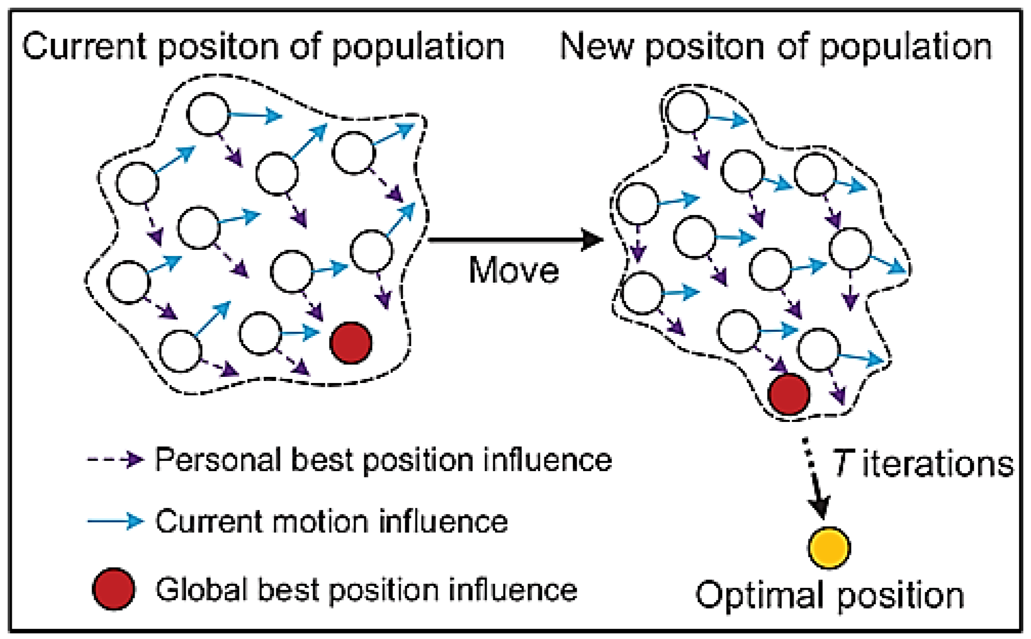
PSO is a computation technique which can be used to optimize a problem by iteratively trying to enhance a proposed solution with regard to a given quality metric (cost function). PSO works to optimize the best selection of parameters by defining candidate solutions as populations for these parameters, and then moving these particles in a search space counting on mathematic formulas by changing the particle’s location and velocity. The motion of each particle is affected by its better location and is driven to achieve the best position in the search space; the best positions are updated to search again for better positions. This is expected to push the swarm to find optimal solutions. PSO was originally defined in [25] as a stylized representation of the motion of organisms in a bird flock or fish school. PSO does not guarantee finding the best solution. More specifically, PSO does not depend on the error gradient; optimization is performed compared with ordinary optimization techniques such as gradient descent and quasi-Newton methods. PSO is used for optimization issues that are partially noisy, irregular, changeable with respect to time, etc.
The basics of the PSO algorithm are that it works depending on a population (named as a swarm) of candidate solutions (named particles). These particles change positions from their current position to new positions around the search space. The process is repeated with the hope of finding a satisfactory solution; however, this is not guaranteed. Figure 2 shows the basic method of PSO.
Formally, let f :   n     be the objective function which must be decreased. The function has an input of a vector of candidate solutions of real numbers, and outputs a real number as a value of the cost function to be minimized. The gradient of f is not known. The aim is to find a position in the space (solution) a for which f ( a )     f ( b ) for all b in the search space, and where position a is the global minimum. Cost functions might be in a form of   h = f ; thus, we need to maximize the function instead of minimizing it [26].
Let S be the total count of particles in the swarm; every particle has its own position and velocity x i     n and v i     n . Let p i be the optimal position of particle   i , and let g be the optimal position of the entire swarm. A basic PSO algorithm is then:
  • For every particle i = 1 ,   ,   S , perform the following steps:
    Start with the position of a particle by a random vector with uniform distribution: x i   ~   U ( b l o ,   b u p ) , where   b u p and b l o are the upper boundary and lower boundaries of the search space, respectively;
    Set the initial value of the particle’s best position to: p i     x i ;
    When ( f ( p i ) < f ( g ) ) , change g     p i ;
    Set the initial value of the particle’s velocity:   v i   ~   U ( | b u p b l o | ,   | b u p b l o | ) .
  • Until a termination condition is met (i.e., the final iteration is met or a solution with adequate objective function value is found):
    For every particle i = 1 ,   ,   S , perform the following steps:
    Choose random numbers: r p ,   r g   ~   U ( 0 , 1 ) ;
    For every d = 1 ,   ,   n , perform the following steps:
    Update the velocity of the particle;
    Update the position of particle:   x i   x i + T i m e v i .
    When ( f ( x i ) < f ( p i ) ) , perform the following steps:
    Update the best-known position of the particle: p i     x i ;
    When   ( f ( x i ) < f ( g ) ) , update the best-known position of the swarm:   g     p i .
  • Now g represents the best-found solution.
In our project, the PSO attempted to find optimal values of ANN weights.

2.3. Artificial Bee Colony (ABC)

The artificial bee colony (ABC) is an optimization algorithm that depends on the intelligent foraging behavior of a honeybee swarm. The ABC algorithm is a swarm-based meta-heuristic algorithm; it was first introduced by Karaboga in 2005 [27] to optimize numeric problems. The main idea was inspired by the smart searching of honeybees. The algorithm specifically depends on the model proposed by Tereshko and Loengarov [28] for searching methods performed by bee colonies. The basic structure contains three important parts: unemployed foraging bees; employed foraging bees; and food sources.
The role of the first two parts is to search for rich sources of food (third part) close to the hive. The structure also defines smart stages of leading of behavior; leading methods are very important for organization and how to collect food. The two stages are:
  • The mobilization of foragers to find and retrieve rich sources of food, which is reconsidered as positive feedback;
  • Foragers neglecting poor food sources, leading to negative feedback.
In summary, ABCs have bees which are named agents; these are smart forager bees with a problem to solve, i.e., smartly finding sources of rich food. To implement ABCs for any problem, we must convert the optimization problem into a problem of finding a solution in the form of searching for the best parameters that make cost functions as minimal as possible. As a result, the agents (smart bees) randomly find some initial solutions for the parameters, and then enhance the parameters iteratively using the following technique: moving to better positions by means of a neighbor search mechanism while abandoning poor solutions.
A global optimization problem can be defined as finding parameters as an array of one dimension, x , which minimizes the cost function [29] f ( x ) :
m i n   f ( x ) ,   x = ( x 1 , , x i , , x n 1 , x n ) R n  
It has some constraints, as follows:
l i x i u i ,   i = 1 , , n
Subject to:
  g j ( x ) 0 ,   f o r   j = 1 , , p
  h j ( x ) = 0 ,   f o r   j = p + 1 , , q
f ( x ) is defined on a search space, S , which has dimensions of n in R n   ( S R n ) . There are limits for each variable, lower and upper: l i and   u i , respectively. In ABCs, there are three groups of bees:
  • Employed: which are associated with finding specific sources of food;
  • Onlookers: which watch the movements of Employed bees in the hive to select sources of foods;
  • Scouts: which randomly look for sources of food.
Scouts and Onlookers are also called Unemployed bees. Initially, Scout bees work to find all food source positions. Thereafter, Onlooker bees and Employed bees test the nectar of food sources that are discovered by Scout bees. This is a continuous process until all sources are exhausted. Employed bees whose food sources have been exhausted become Scout bees.
In ABCs, the location of food sources is a potential solution, and the quantity of nectar in this source considers the quality (fitness) of the solution [29].
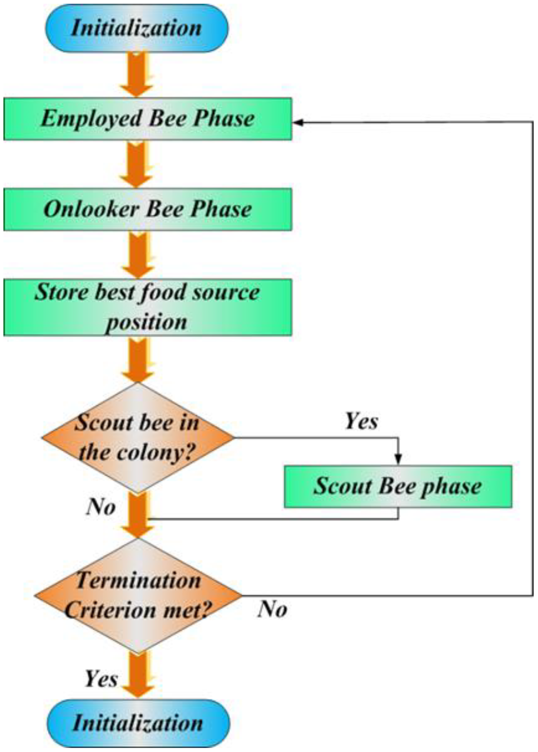
The general flowchart of the ABC method is as follows:
  • Initialization Phase
  • REPEAT
    • Employed Bees Phase
    • Onlooker Bees Phase
    • Scout Bees Phase
    • Memorize the best solution achieved so far
  • UNTIL (Cycle = Maximum Cycle Number)
All necessary parameters are initialized with random values as follows ( m = 1 M ,   M :   p o p u l a t i o n   s i z e ) by Scout bees, and the control parameters are set. The following definition might be used for initialization purposes:
x m i = l i + r a n d ( 0 , 1 ) × ( u i l i )  
where l i and u i are the lower and upper bounds of parameter     x m i , respectively.
Employed bees search for new food sources ( υ m ) with the condition of finding more nectar within the neighborhood of the food source x m i in their memory. After they find a source of food, they check its quality (fitness). They might choose a neighbor source of food υ m by the following formula:
υ m i = x m i + ϕ m i ( x m i x k i )
where x k i is a randomly chosen source, i is also selected randomly, and ϕ m i is a random term in the range   [ a , a ] .
The quality value of the solution,   F m ( x m ) , can be calculated to minimize problems using the subsequent equation:
F m ( x m ) = { 1 1 + F m ( x m ) i f F m ( x m ) 0   1 + a b s ( F m ( x m ) ) i f F m ( x m ) 0 }
F m   is an objective function value of solution x m .
Smart Employed bees share information details about sources of food with smart Onlooker bees which are waiting in the hive. Smart Onlooker bees use the shared information with probabilities from the fitness function F m to choose their food sources. Fitness-based selection methods might be used, such as the roulette wheel selection method [30].
The probability p m that explains which x m   should be chosen can be calculated by:
p m = F m ( x m ) m = 1   M F m ( x m )    
After Onlooker bees choose the location of food   x m , a neighborhood source,   υ m is defined by Equation (6) and its performance is calculated. It is in the phase of Employed bees; therefore, greedy selection is applied between υ m and   x m .
Solutions of Employed bees cannot be enhanced by a specific number of tries, defined by the user of the ABC algorithm and called the “abandonment condition”. Then, the converted Scouts begin to find new solutions. If solution x m is being abandoned, the new solution is found by Scouts which were previously Employed bees of   x m , as can be calculated by Equation (5). Hence, those sources which were initially poor or have been made poor by exploitation are abandoned, and negative feedback behavior arises to balance the positive feedback.
The flowchart in Figure 3 shows the stages that are explained above.
There are many other methods for optimization that can be used, such as in [31,32,33]. Some of them are used for hybrid forecasting for hour-ahead solar power prediction. Gradient-descent optimization with forecasting algorithm: gradient-descent optimization might be used for initial parameters initialization of an ANN. Others depend on global hybrid ABC; other optimization algorithms are reported in [34,35], such as grid-search and the fruit fly optimization algorithm (FOA).

2.4. Validation Metrics

Suppose a vector of real value Y and a vector of predicted value   Y ^ . The length of the vectors is N.

2.4.1. Mean Square Error

M S E = 1 N i = 1 N ( Y i     Y ^ i ) 2

2.4.2. Mean Absolute Percentage Error

M A P E = 1 N i = 1 N | Y i     Y ^ i Y i |

2.4.3. Coefficient of Determination R 2

R 2 = 1 R S S T S S
where RSS is the residual sum of squares and TSS is the total sum of squares.
R S S = i = 1 N ( Y i     Y ^ i ) 2
T S S = i = 1 N ( Y i Y ¯ ) 2
Here, Y ¯   is the mean of Y i .

3. Simulation Results

3.1. Data Processing

The features are: ‘DATE’, ‘TIME’, ‘Humidity’, ‘Pressure’, ‘Tempsur’, ‘TempAmp’, ‘SolarV’, ‘SolarC’, ‘SolarIr’, and ‘SolarP’. Some columns contain the character “:”. This issue is handled and rows with NaN values were deleted. The label of data is the last column ‘SolarP’. Other columns were gathered as the features or inputs for the tested algorithm.
The setup for all methods is shown below:
For GA: Tolerance function: 1 × 10 10 , number of generation: 200, cost function desired limit 1 × 10 7 .
For PSO: Personal learning coefficient: 0.8 , population size: 150, iterations: 500, range of values [–5,5].
For ABC: Tolerance function:   1 × 10 8 , iterations: 1000.

3.2. Traditional ANN

We define the number of neurons as 18; ANN is a traditional feedforward network.
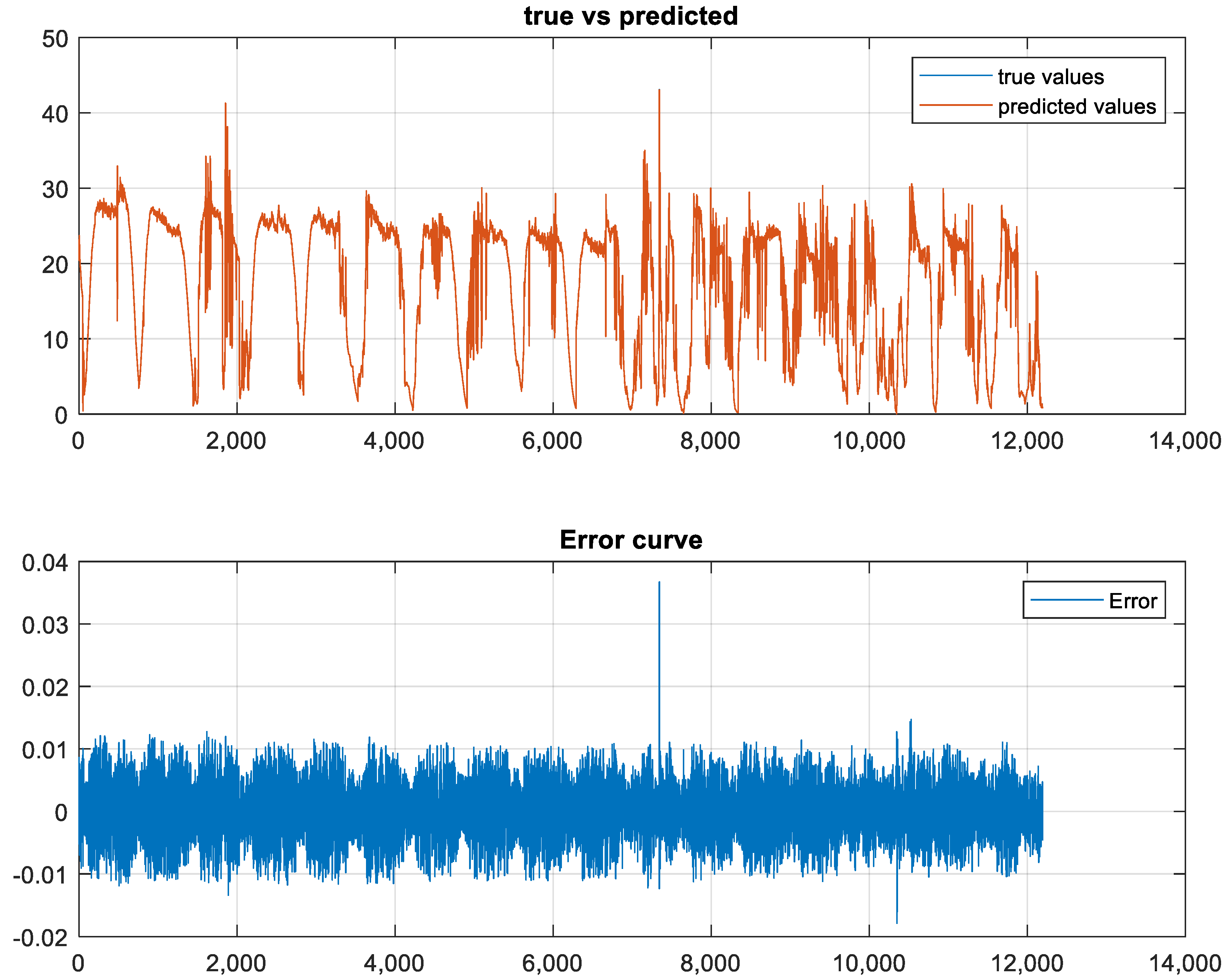
As shown in Figure 4 and Figure 5, the final error is around zero. During training, the error is 0.0252%. The error gradient is about 0.0001.

3.3. ANN with the Genetic Algorithm

We defined the same network as previously, with 18 neurons. Then, we obtained the weights from the ANN. We defined the GA options: the number of generations was 200 and the initial range for the population was [−2, +2], with a minimum value of fitness function and tolerance function. We passed the weights as inputs for the GA and the cost function was the mean square error. The algorithm ended when no enhancement could be reached in the quality function within a period of time in seconds equal to the stall time limit. The process is shown in Table 1.
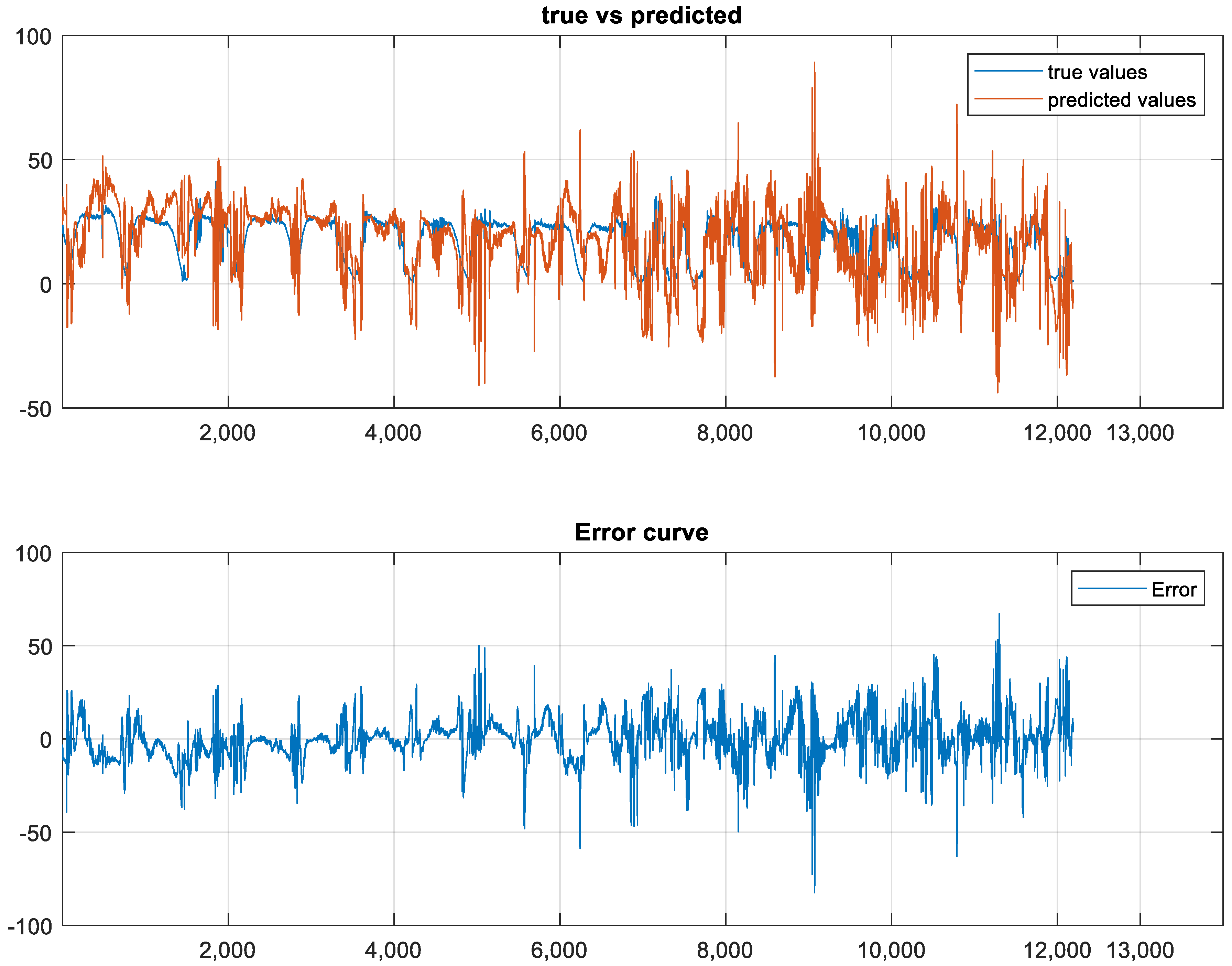
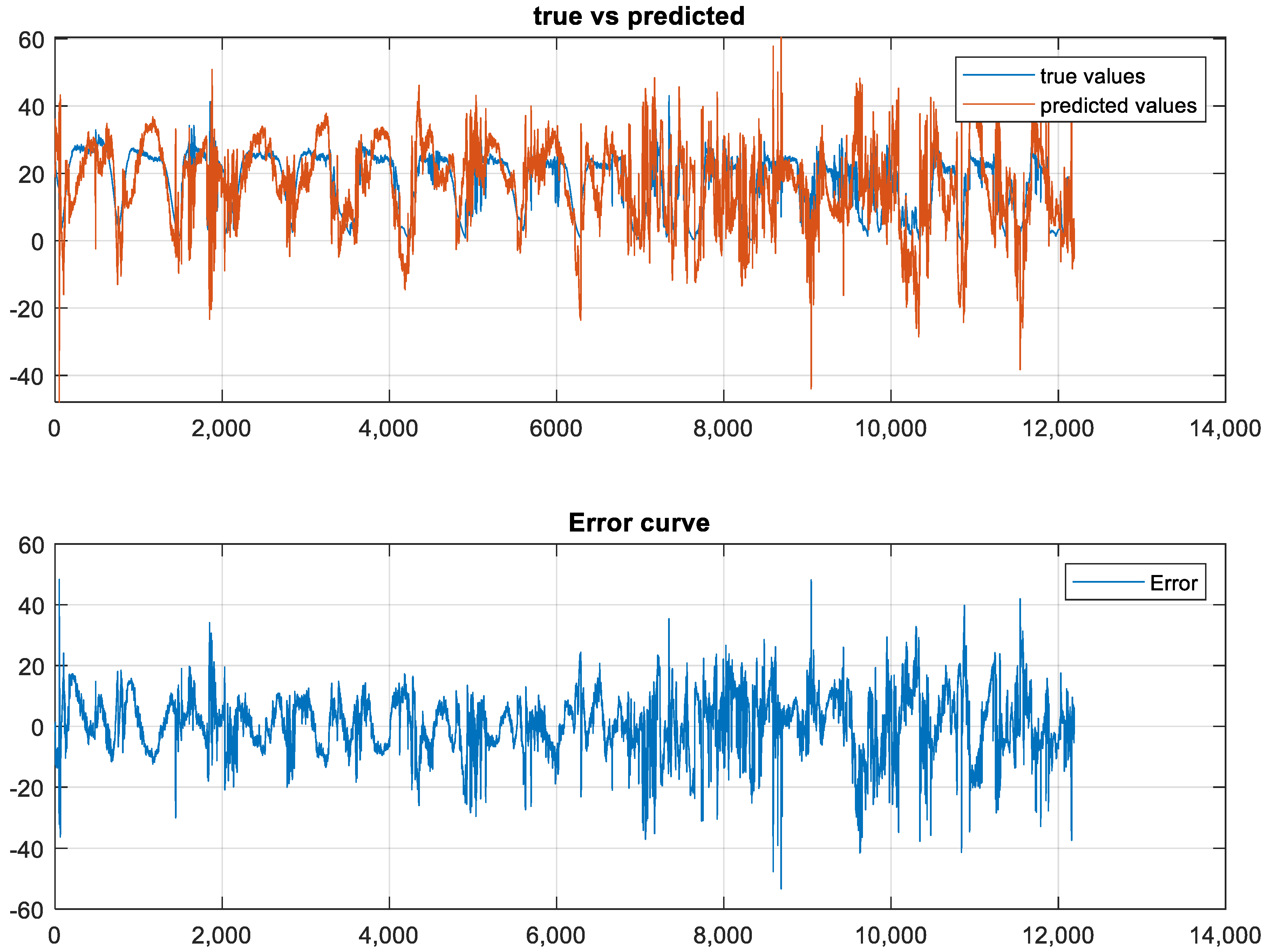
The final results are shown below in Figure 6 and Figure 7 for the first and second tests.

3.4. ANN with PSO

Validation of the PSO–ANN is shown in Figure 8.
Table 2 shows changes in the first 10 epochs.

3.5. ANN with ABC

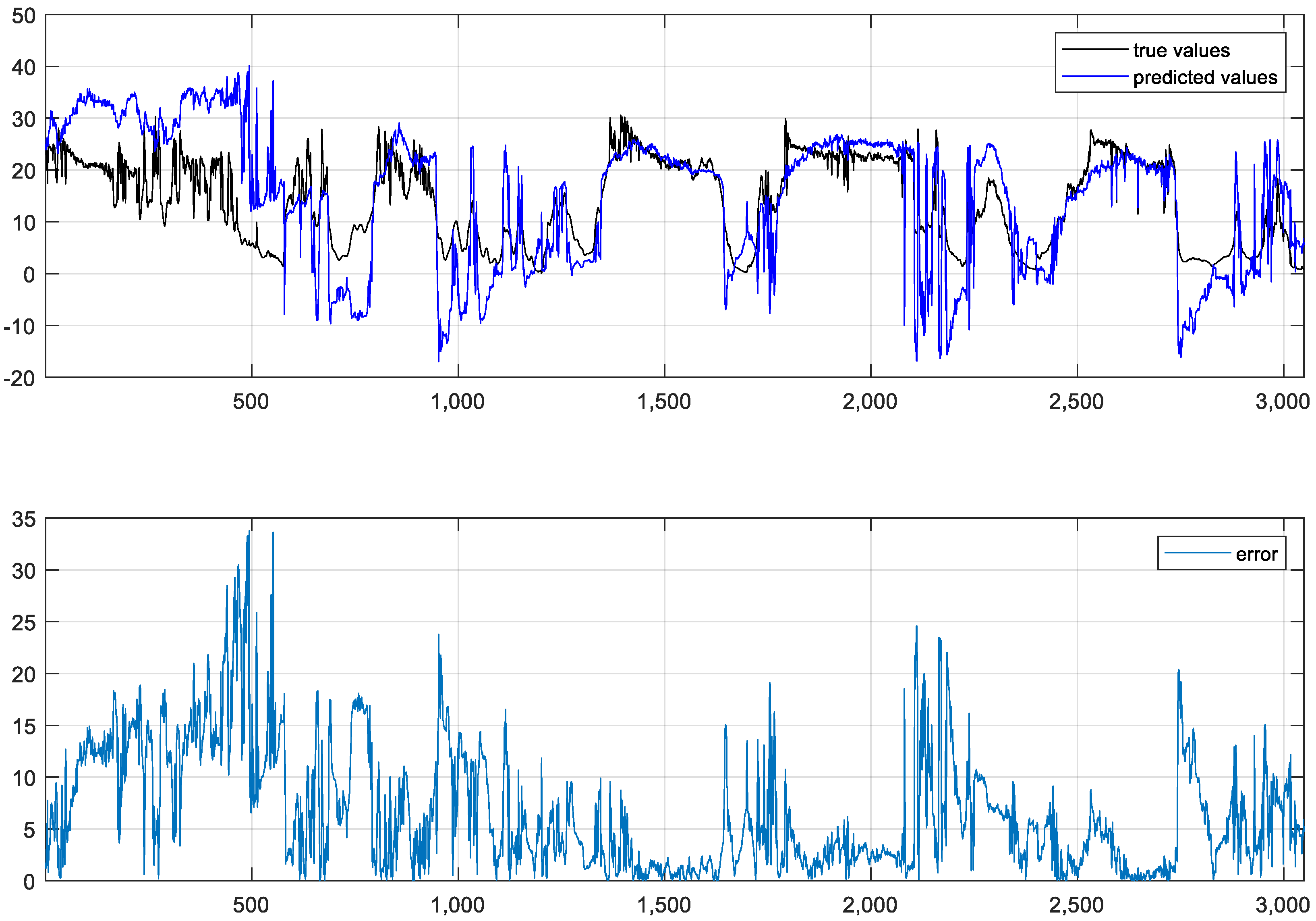
In this algorithm, a splitting dataset was implemented. The dataset was split into test and train parts; the results are shown in Figure 9 and Figure 10.

3.6. Results Comparisons

All methods are compared in Table 3.
The results show that the traditional NN with basic finding methods is the best. PSO–ANN is the best between PSO–ANN, GA–ANN, and ABC–ANN. Each study has its own dataset, the comparison would not be valuable because it is not the same dataset. However, we can tell that our methods have achieved a great accuracy, especially PSO-ANN, since the accuracy was 99.71%. The dataset can be shared with other researchers to obtain a comparison in the future

4. Conclusions

In this study, implementation for a solar power output was performed with ANN and three different optimization algorithms: genetic algorithm, particle swarm optimization, and artificial bee colony. The results showed that the PSO is best algorithm for finding optimal parameters of ANNs. Its performance (with respect to R2) was 99.71% with minimum MSE and MAPE values. In the future, these algorithms can be analyzed and more details about their parameters can be determined. Utilizing more features of the datasets can also enhance the model of prediction.

Author Contributions

The authors have searched and tested many optimization algorithms to enrich fields of optimization and solar photovoltaic power estimation. This search is aimed to be a guide for researchers of these fields. All authors have read and agreed to the published version of the manuscript.

Funding

This research received no external funding.

Informed Consent Statement

The authors consent for publication.

Data Availability Statement

The dataset is available to the public.

Conflicts of Interest

The authors declare no conflict of interest.

References

  1. Filik, Ü.B.; Filik, T.; Gerek, Ö.N. New electric transmission systems: Experiences from Turkey. In Handbook of Clean Energy Systems; John Wiley & Sons, Ltd.: Hoboken, NJ, USA, 2015; pp. 1–13. [Google Scholar]
  2. Zazoum, B. Solar photovoltaic power prediction using different machine learning methods. Energy Rep. 2021, 8, 19–25. [Google Scholar] [CrossRef]
  3. El Hendouzi, A.; Bourouhou, A. Solar Photovoltaic Power Forecasting. J. Electr. Comput. Eng. 2020, 2020, 8819925. [Google Scholar] [CrossRef]
  4. Nordell, B. Thermal pollution causes global warming. Glob. Planet. Chang. 2003, 38, 305–312. [Google Scholar] [CrossRef]
  5. Peters, K. COVID-19: How GOGLA is Helping the Off-Grid Solar Industry Deal with the Crisis. Available online: https://www.gogla.org/about-us/blogs/covid-19-how-gogla-ishelping-the-off-grid-solar-industry-deal-with-the-crisis (accessed on 5 October 2022).
  6. Burnett, J.W.; Hefner, F. Solar energy adoption: A case study of South Carolina. Electr. J. 2021, 34, 106958. [Google Scholar] [CrossRef]
  7. Eroğlu, H. Effects of Covid-19 outbreak on environment and renewable energy sector. Environ. Dev. Sustain. 2020, 23, 4782–4790. [Google Scholar] [CrossRef] [PubMed]
  8. Yang, M.; Huang, X. An Evaluation Method of the Photovoltaic Power Prediction Quality. Math. Probl. Eng. 2018, 2018, 9049215. [Google Scholar] [CrossRef] [Green Version]
  9. Jiang, H.; Lu, L.; Sun, K. Experimental investigation of the impact of airborne dust deposition on the performance of solar photovoltaic (PV) modules. Atmos. Environ. 2011, 45, 4299–4304. [Google Scholar] [CrossRef]
  10. Pi, M.; Jin, N.; Chen, D.; Lou, B. Short-Term Solar Irradiance Prediction Based on Multichannel LSTM Neural Networks Using Edge-Based IoT System. Wirel. Commun. Mob. Comput. 2022, 2022, 2372748. [Google Scholar] [CrossRef]
  11. Cheng, Z.; Liu, Q.; Zhang, W. Improved Probability Prediction Method Research for Photovoltaic Power Output. Appl. Sci. 2019, 9, 2043. [Google Scholar] [CrossRef] [Green Version]
  12. Hu, K.; Cao, S.; Wang, L.; Li, W.; Lv, M. A new ultra-short-term photovoltaic power prediction model based on ground-based cloud images. J. Clean. Prod. 2018, 200, 731–745. [Google Scholar] [CrossRef]
  13. Jung, Y.; Jung, J.; Kim, B.; Han, S. Long short-term memory recurrent neural network for modeling temporal patterns in long-term power forecasting for solar PV facilities: Case study of South Korea. J. Clean. Prod. 2019, 250, 119476. [Google Scholar] [CrossRef]
  14. Arias, M.B.; Bae, S. Solar Photovoltaic Power Prediction Using Big Data Tools. Sustainability 2021, 13, 13685. [Google Scholar] [CrossRef]
  15. Agga, A.; Abbou, A.; Labbadi, M.; El Houm, Y.; Ali, I.H.O. CNN-LSTM: An efficient hybrid deep learning architecture for predicting short-term photovoltaic power production. Electr. Power Syst. Res. 2022, 208, 107908. [Google Scholar] [CrossRef]
  16. Cho, M.-Y.; Lee, C.-H.; Chang, J.-M. Application of Parallel ANN-PSO to Hourly Solar PV Estimation. Preprints 2021, 2021100112. [Google Scholar]
  17. Geetha, A.; Santhakumar, J.; Sundaram, K.M.; Usha, S.; Thentral, T.T.; Boopathi, C.; Ramya, R.; Sathyamurthy, R. Prediction of hourly solar radiation in Tamil Nadu using ANN model with different learning algorithms. Energy Rep. 2021, 8, 664–671. [Google Scholar] [CrossRef]
  18. Lopes, S.M.A.; Cari, E.P.T.; Hajimirza, S. A Comparative Analysis of Artificial Neural Networks for Photovoltaic Power Forecast Using Remotes and Local Measurements. J. Sol. Energy Eng. 2021, 144, 021007. [Google Scholar] [CrossRef]
  19. Hashunao, S.; Sunku, H.; Mehta, R.K. Modelling and Forecasting of Solar Radiation Data: A Case Study. In Modeling, Simulation and Optimization; Springer: Berlin/Heidelberg, Germany, 2021; pp. 1–13. [Google Scholar]
  20. Das, R.; Singh, K.; Akay, B.; Gogoi, T.K. Application of artificial bee colony algorithm for maximizing heat transfer in a perforated fin. J. Process Mech. Eng. 2018, 232, 38–48. [Google Scholar] [CrossRef]
  21. Das, R.; Akay, B.B.; Singla, R.K.; Singh, K. Application of artificial bee colony algorithm for inverse modelling of a solar collector. Inverse Probl. Sci. Eng. 2016, 25, 887–908. [Google Scholar] [CrossRef]
  22. Wang, S.C. Artificial Neural Network. In Interdisciplinary Computing in Java Programming; Springer: Boston, MA, USA, 2003; pp. 81–100. [Google Scholar]
  23. Gupta, N. Artificial neural network. Netw. Complex Syst. 2013, 3, 24–28. [Google Scholar]
  24. Kramer, O. Genetic algorithms. In Genetic Algorithm Essentials; Springer: Cham, Switzerland, 2017; pp. 11–19. [Google Scholar]
  25. Alam, T.; Qamar, S.; Dixit, A.; Benaida, M. Genetic algorithm: Reviews, implementations, and applications. arXiv 2020, arXiv:2007.12673. [Google Scholar] [CrossRef]
  26. Kumar, M.; Husain, D.; Upreti, N.; Gupta, D. Genetic Algorithm: Review and Application. 2010. Available online: https://ssrn.com/abstract=3529843 (accessed on 10 October 2022).
  27. Kennedy, J.; Eberhart, R. Particle swarm optimization. In Proceedings of the ICNN’95-International Conference on Neural Networks, Perth, WA, Australia, 27 November–1 December 1995; Volume 4, pp. 1942–1948. [Google Scholar]
  28. Chen, Z.; Li, X.; Zhu, Z.; Zhao, Z.; Wang, L.; Jiang SRong, Y. The optimization of accuracy and efficiency for multistage precision grinding process with an improved particle swarm optimization algorithm. Int. J. Adv. Robot. Syst. 2020, 17, 1729881419893508. [Google Scholar] [CrossRef] [Green Version]
  29. Karaboga, D. An Idea Based on Honey Bee Swarm for Numerical Optimization; Technical Report-tr06; Erciyes University, Engineering Faculty, Computer Engineering Department: Talas/Kayseri, Turkey, 2005; Volume 200, pp. 1–10. [Google Scholar]
  30. Karaboga, D.; Basturk, B. A powerful and efficient algorithm for numerical function optimization: Artificial bee colony (ABC) algorithm. J. Glob. Optim. 2007, 39, 459–471. [Google Scholar] [CrossRef]
  31. Shah, H.; Ghazali, R.; Nawi, N.M.; Deris, M.M. Global hybrid Artificial bee colony algorithm for training artificial neural networks. In Proceedings of the International Conference on Computational Science and Its Applications, Salvador de Bahia, Brazil, 18–21 June 2012; Springer: Berlin/Heidelberg, Germany, 2012; pp. 87–100. [Google Scholar]
  32. Goldberg, D.E.; Deb, K. A comparative analysis of selection schemes used in genetic algorithms. In Foundations of Genetic Algorithms; Elsevier: Amsterdam, The Netherlands, 1991; Volume 1, pp. 69–93. [Google Scholar]
  33. Asrari, A.; Wu, T.X.; Ramos, B. A Hybrid Algorithm for Short-Term Solar Power Prediction—Sunshine State Case Study. IEEE Trans. Sustain. Energy 2016, 8, 582–591. [Google Scholar] [CrossRef]
  34. Bao, Y.; Liu, Z. A Fast Grid Search Method in Support Vector Regression Forecasting Time Series; Springer: Berlin/Heidelberg, Germany, 2006; pp. 504–511. [Google Scholar]
  35. Li, H.; Guo, S.; Zhao, H.; Su, C.; Wang, B. Annual electric load forecasting by a least squares support vector machine with a fruit fly optimization algorithm. Energies 2012, 5, 4430–4445. [Google Scholar] [CrossRef]
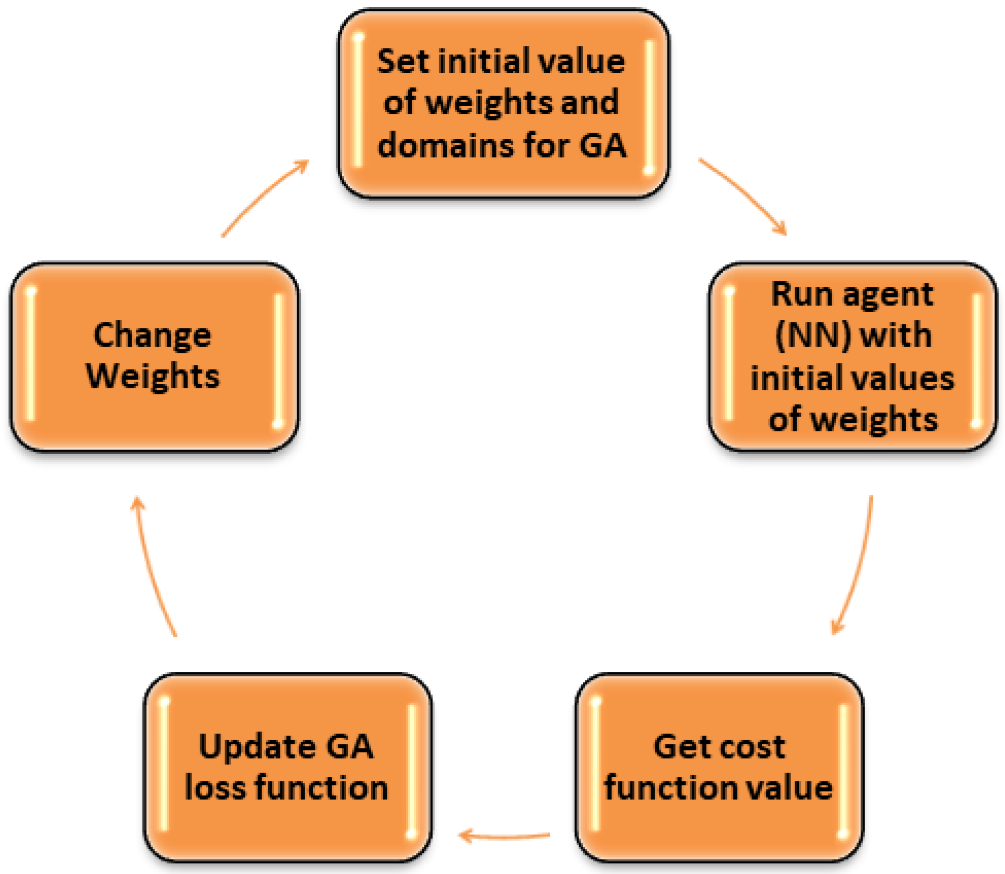
Figure 1. Loop of the GA process.
Energies 15 08669 g001
Figure 2. Schematic of a basic PSO and the move.
Energies 15 08669 g002
Figure 3. Flowchart of ABC algorithm.
Energies 15 08669 g003
Figure 4. Training process of pure ANN with any optimization.
Energies 15 08669 g004
Figure 5. Error and output of ANN results on real data.
Energies 15 08669 g005
Figure 6. Error and output of GA–ANN results (first test).
Energies 15 08669 g006
Figure 7. Error and output of GA–ANN results (second test).
Energies 15 08669 g007
Figure 8. Error and output of PSO–ANN results.
Energies 15 08669 g008
Figure 9. Results of ABC–ANN for testing part.
Energies 15 08669 g009
Figure 10. Results of ABC–ANN for training part.
Energies 15 08669 g010
Table 1. The cost function process of the GA–ANN.
GenerationBest Cost FunctionMean Cost Function
110.61445.6
210.61617.2
310.61725.2
410.61726.6
510.61819.7
610.61896.7
710.61795.7
810.61753.2
910.61771.9
1010.61761.1
119.497834.7
129.464828.7
139.438775.7
147.963733.7
157.518772.8
Table 2. Best function during the process of the PSO–ANN.
IterationBest Cost Function
143.4098
243.4098
318.8759
41.368
51.368
61.368
71.368
81.368
91.368
101.368
Table 3. Numerical comparison of methods.
MSEMAPER2
ANN0.000020340.000405141
GA–ANN6.14400.67900.4841
PSO–ANN0.46070.05240.9971
ABC–ANN35.14280.78900.5004
Publisher’s Note: MDPI stays neutral with regard to jurisdictional claims in published maps and institutional affiliations.