Prediction of Carbon Dioxide Emissions in China Using Shallow Learning with Cross Validation

Abstract

Accurately measuring carbon dioxide (CO₂) emissions is critical for effectively implementing carbon reduction policies, and China’s increased investment in reducing CO₂ emissions is expected to significantly impact the world. In this study, the potential of shallow learning for predicting CO₂ emissions was explored. Data included CO₂ emissions, renewable energy consumption, and the share of primary, secondary, and tertiary industries in China from 1965 to 2021. These time-series data were converted into labeled sample data using the sliding window method to facilitate a supervised learning model for CO₂ emission prediction. Then, different shallow learning models with k-fold cross-validation were used to predict China’s short-term CO₂ emissions. Finally, optimal models were presented, and the important features were identified. The key findings were as follows. (1) The combined model of RF and LASSO performed best at predicting China’s short-term CO₂ emissions, followed by LASSO and SVR. The prediction performance of RF was very fragile to the window width. (2) The sliding window method is used to convert time series predictions into supervision learning problems, and historical data can be used to predict future carbon dioxide emissions. To ensure that the feature data are real, the model can predict CO₂ emissions for up to six years ahead. (3) Cross-validation and grid search were critical for optimizing China’s CO₂ emissions prediction with small datasets. (4) By 2027, carbon dioxide emissions will continue to grow and reach 10.3 billion tons. It can be seen that the task of China to achieve its carbon peak on schedule is very heavy. The results indicate that an increase in renewable energy consumption and adjustments in industrial structure will continue to play an important role in curbing China’s CO₂ emissions.

1. Introduction

Sharp increases in carbon dioxide (CO₂) emissions strengthen the greenhouse effect, leading to an ongoing increase in the global average temperature. The average annual global emissions of greenhouse gases from 2010 to 2019 were at the highest level in human history. Since then, the growth rate has slowed. Global greenhouse gas (GHG) emissions are expected to peak by 2025 to meet the goal of limiting global warming to 1.5 °C by the end of the century. Specifically, annual CO₂ emissions are expected to fall by approximately 48% by 2030 and reach net zero by 2050 [1].

As a developing country, China faces the dual task of developing its economy and protecting the environment. In the past two decades, China’s economy has developed rapidly, and because economic development depends on energy consumption [2,3], China has become a large energy consumer and carbon emitter [4,5]. In 1990, China’s emissions were less than one-quarter of the total of the world’s developed countries. Since 2006, however, China has been the world’s largest carbon emitter [6,7].

China’s CO₂ emissions mainly come from electricity generation [8,9], industry [10], construction [11,12], transportation [13,14], and agriculture [15]. Of these, electricity and industry are the two major high-emission sectors, accounting for more than 70% of the total emissions. Thermal power generation currently dominates China’s power structure. The main ways to reduce carbon in the power industry include reducing the proportion of coal power; accelerating the development of non-fossil energy, such as wind and photovoltaic power; and building a clean, low-carbon, safe, and efficient energy system. Second, achieving a low-carbon economy requires adjusting the industrial structure. This includes increasing the proportion of the service industry, which provides economic activity at low consumption and emission levels, and reducing the proportion of the manufacturing industry, which has high consumption and emission levels.

China’s CO₂ emission reduction effect and environmental protection policies are expected to significantly impact the global climate [16]. As a signatory to the Paris Agreement, China had committed to achieving a carbon peak by 2030 [17] and achieving carbon neutrality by 2060. However, as a fast-growing carbon polluter, China’s commitment holds particular weight, because achieving a carbon peak and carbon neutrality involves technological and economic development, and China’s CO₂ emissions per unit of gross domestic product (GDP) are still at the highest level in the world. To achieve its carbon peak and neutrality targets, it is vital to accurately predict China’s future CO₂ emissions and identify the factors influencing those CO₂ emissions, to inform corresponding emission reduction policies.

2. Literature Review

This literature review section is organized as follows. First, the prediction of CO₂ emissions is reviewed. Second, studies on the causality among industrial structure, energy consumption, and CO₂ emissions are reviewed. Finally, the application of machine learning (ML) to predict CO₂ emissions is reviewed. The literature review focuses special attention on research in China.

2.1. Studies on CO₂ Emission Predictions

Grey prediction models are widely used in CO₂ emission forecasting. A multi-variable grey model (GM(1,N) model), based on a linear time-varying parameters discrete grey model (TDGM(1,N)), was established to predict the CO₂ emissions from Anhui Province [18]. The key challenge in forecasting CO₂ emissions is investigating the dynamic lag relationships. As such, an enhanced dynamic time-delay discrete grey forecasting model was proposed to predict outcomes for systems with dynamic time-lag effects. The model was used to significantly improve the fitting and prediction performance, using CO₂ emissions data from 1995 to 2017 [19].

Scenario analysis is widely used to predict long-term CO₂ emissions. Zhang et al. (2021) used regression analysis to quantify the impact of three factors on CO₂ emissions: Total population, educational attainment, and per capita GDP. Then, CO₂ emission predictions for 2018 to 2100 were developed using these three factors across different scenario settings, involving multiple model parameters and explanatory variables [20]. Li et al. (2020) used the Generalized Dividing Index Method to quantify the contribution rate of each factor influencing the CO₂ emissions of China’s construction industry and predicted the carbon peaks of China’s construction industry in three scenarios [21].

2.2. Studies on the Factors Influencing CO₂ Emissions

The existing literature has analyzed the effect of industrial structure and economic development on CO₂ emissions. Zheng et al. (2019) applied the logarithmic mean Divisia index (LMDI) to estimate seven socioeconomic drivers impacting changes in CO₂ emissions in China since 2000. The results showed that industrial structure and energy mix resulted in emissions growth in some regions, but these two drivers led to emission reductions at the national level [22]. Dong et al. (2020) applied the extended STIRPAT decomposition model, Tapio decoupling model, and grey relation analysis to analyze the relationships between CO₂ emissions, industrial structure, and economic growth in China from 2000 to 2017. The results showed that the key steps needed for China to reach its carbon peak goal are accelerating the achievement of a clean energy structure, strengthening the strength and speed of industrial structure adjustment, and reducing the dependence on fossil energy [23]. Panel econometric techniques were applied to examine the nexus between CO₂ emissions, urbanization level, and industrial structure in North China over the period of 2004–2019. The empirical results support the long-term equilibrium relationship between CO₂ emissions and industrial structure in North China, indicating that industrial structure significantly impacts CO₂ emissions [24].

The interaction between renewable energy and CO₂ emissions is also a key research direction. Dong et al. (2017) used panel unit root, cointegration, causality tests, and the augmented mean group (AMG) estimator to investigate the nexus between per capita CO₂ emissions, gross domestic product (GDP), and natural gas and renewable energy consumption in a 1985–2016 sample of BRICS countries (defined as Brazil, Russia, India, China, and South Africa). The results found that natural gas and renewable energy consumption lowers CO₂ emissions [25]. Zheng et al. (2021) analyzed the influence of renewable energy generation in China on CO₂ emissions using a quantile regression model and path analysis of inter-provincial panel data from 2008 to 2017. The results found that renewable energy has a less direct effect on CO₂ emissions, but energy intensity and GDP per capita inhibit CO₂ emissions [26]. Abbasi et al. (2022) applied novel dynamic ARDL simulations and Frequency Domain Causality (FDC) models to analyze the environmental factors influencing China’s CO₂ emissions from 1980 to 2018. The results showed that renewable energy consumption is crucial for achieving sustainable environmental goals, despite there being a short-term detrimental impact on CO₂ emissions [27].

2.3. Studies on Using ML for CO₂ Emissions

ML applies data and experience to automatically improve computer algorithms using probability theory, statistics, approximation theory, and complex algorithms. For random, high-dimensional, nonlinear, and feedback complex systems, ML uses different core algorithms to identify and predict the patterns of the complex system.

Sun and Ren (2021) combined ensemble empirical mode decomposition (EEMD) and the backpropagation neural network based on particle swarm optimization (PSOBP) to develop short-term univariate predictions of CO₂ emissions in China [28]. However, univariate predictions only mine CO₂ emissions data and do not consider the influence of other factors on CO₂ emissions.

To address this, multivariate time-series forecasting is used to predict CO₂ emissions. The least absolute shrinkage and selection operator (LASSO) and principal component analysis (PCA) are used to select features. Then, support vector regression (SVR) and differential evolution-gray wolf optimization (DE-GWO) are used to improve the prediction accuracy of China’s CO₂ emissions. Results using these approaches show that coal and oil consumption, plate glass, pig iron, and crude steel production are important factors affecting CO₂ emissions, and the DE-GWO optimized SVR has an effective level of prediction accuracy [29]. The XGBoost model has also been used to predict the CO₂ emissions of expanding megacities. Under the synergistic effect of multiple factors, population, land size, and GDP are still the primary forces driving CO₂ emissions [30]. A three-layer perceptron neural network (3-layer PNN) performed well in predicting transportation CO₂ emission in Zhuhai, China [31]. The Autoregressive Integrated Moving Average (ARIMA) was used to predict CO₂ emissions from four Chinese provinces over three future years using data from 1997 to 2017 [32]).

ML is also used to analyze the correlation between feature variables. A different study applied a Causal Direction from Dependency (D2C) algorithm to investigate the relationships between coal, solar, wind, and CO₂ emissions [33]. Using data from 1990 to 2014 in China, the long short-term memory (LSTM) method was applied to investigate the impact of energy consumption, financial development (FD), GDP, population, and renewable energy on CO₂ emissions and forecast emission trends [34].

The literature review revealed three main points and research gaps. First, many models based on grey predictions have been used to predict CO₂ emissions. However, instead of using raw data, grey predictions use a series of generated data that approximate exponential laws. Therefore, grey prediction requires high smoothness in the original data series. When the original data column has poor smoothness, the prediction accuracy of the grey prediction model is not high. Although scenario analysis is suitable for predicting long-term CO₂ emissions, the accuracy of prediction results is limited by the ability of decision makers to develop scenarios and the validity of data.

Second, some studies have investigated the impact of economic growth and industrial structure on CO₂ emissions, while others have studied and investigated the relationship between renewable energy, economic growth, and CO₂ emissions. However, few studies have put CO₂ emissions, industrial structure, and renewable energy consumption into a single research framework to forecast China’s CO₂ emissions.

Third, some studies have applied ML to predict CO₂ emission data in univariate time series, without considering industrial structure and renewable energy, which are closely related to CO₂ emissions. Some studies have conducted multivariate time predictions for CO₂ emissions in a specific industry. However, few studies have used ML to predict China’s CO₂ emissions in a multivariable time series.

The three research gaps listed above exhibit where this study finds its objective. With respect to the methodology, we applied shallow learning to predict China’s future short-term CO₂ emissions without requiring the data samples to meet strict statistical properties. This improved the prediction ability of the model using realistic data. With respect to practicability, we converted the time-series data into supervised learning data with labels and used historical data to predict future data to mitigate the unavailability of sample data. Finally, from an empirical perspective, we integrated renewable energy with the industrial structure and CO₂ emissions in a research framework to construct a multivariate forecasting model. This model has a stronger forecasting ability than univariate time series, and effectively identified the impact of industrial structure and renewable energy on CO₂ emissions.

3. Data and Methodology

3.1. Data Collection

This study forecasted China’s CO₂ emissions by focusing on two areas: Industrial structure and renewable energy consumption. The proportion of primary, secondary, and tertiary industries reflects industrial structure. The data span from 1965 to 2021 and include data from the company BP’s statistical review of world energy (https://www.bp.com/en/global/corporate/energy-economics/statistical-review-of-world-energy/downloads.html, accessed on 10 June 2022) on CO₂ emission and renewable energy, and other data from the National Bureau of Statistics (http://www.stats.gov.cn/, accessed on 10 June 2022) in China.

Figure 1 shows China’s CO₂ emissions from 1965 to 2021. Before 2000, the growth rate of China’s CO₂ emissions was basically stable at approximately 5%. After China’s accession to the World Trade Organization in 2001, the rapid development of China’s economy led to a sharp rise in CO₂ emissions. From 2001 to 2010, China’s CO₂ emissions grew as fast as its gross domestic product (GDP), at one point reaching 18%. In 2005, China became the world’s largest emitter of carbon dioxide. After 2011, China began to implement relatively strict environmental protection policies, so the growth rate of carbon emissions began to decline, and basically remained below 5%.

The proportion of primary, secondary, and tertiary industries in China’s GDP shows the trend of China’s industrial structure. Primary industry refers to agriculture, forestry, animal husbandry, and fishery (excluding professional and auxiliary activities of agriculture, forestry, animal husbandry, and fishery). Secondary industry refers to mining, manufacturing, electricity, heat, gas and water production and supply, and construction. Tertiary industry represents the service industry and refers to other industries not encompassed by the other two. Since 1970, SI has been stable at approximately 40%, with little change. PI decreased from 37% in 1965 to 7% in 2021, while TI increased from 27% in 1965 to 53%, as shown in Figure 2.

Figure 3 shows China’s renewable energy consumption from 1965 to 2021. In 2006, China entered a period of rapid development of renewable energy with a growing market size. Remarkable progress has been made in the development and utilization of renewable energy, with the cumulative installed capacity of hydropower, wind power, photovoltaic power, and other energy sources ranking first in the world. Since 2011, plans at the national level have given a strong boost to renewable energy. In 2021, China’s renewable energy utilization reached 750 million tons of standard coal, accounting for 14.2 percent of the total primary energy consumption, and reduced carbon dioxide emissions by approximately 1.95 billion tons, laying the foundation for achieving the “double carbon” target.

3.2. Methodology

ML involves shallow and deep learning. Shallow learning usually has no hidden layer or only one hidden layer, and approaches include Linear Regression (LR), Ridge, LASSO, SVR, Random Forest (RF), and the Gradient Boosting Decision Tree (GBDT). Shallow learning has a limited ability to express complex functions, limiting its ability to generalize complex problems. In contrast, deep learning increases the depth of network models; approaches include Recurrent Neural Networks (RNN) and Convolutional Neural Networks (CNN). The feature representation of samples in the original space is transformed into a new feature space using layer-by-layer feature transformation to achieve complex function approximation. This highlights the importance of feature learning.

Given how shallow and deep learning work, there are two main differences between them. First, deep learning usually requires more training samples to prevent the over-fitting of deep learning predictions. For small samples, shallow learning has higher prediction accuracy than deep learning [35]. Second, deep learning generally has poor interpretability, due to the transformation of feature variables. As a deep learning model used to predict time series, LSTM has these problems. In contrast, shallow learning models are explanatory; however, these supervised learning models do not effectively address time series regression.

This study, therefore, reconstructed time series data for CO₂ emissions, and then converted the time-series-based forecasting into a supervised learning problem. Considering the small sample data set and the interpretability, the shallow learning was used to predict CO₂ emissions in China.

3.2.1. Modeling Time Series for Supervised Learning

The first step in this study was transforming time-series data predictions into a supervised learning problem. First, the data for the supervised learning problem were labeled, and the algorithm was continuously iterated to predict the training data. By comparing the predicted label with the real label, the model parameters were updated and modified to minimize the defined loss function. When the algorithm reached an acceptable performance level, the learning stopped. The sliding window method was used to transform the time series data into supervised learning problems.

In general, the sliding window method uses the value of the previous time point to predict the value of the next time point. The number of time points is called a window width. However, before sliding the time windows to transform the time-series data into supervised learning data, it is important to define the following notations.

Definition 1.

Suppose that a multivariate time series has T time steps, each of which has M observations. Let ${\mathit{x}}_{\mathit{t}}$ be the feature vector at time t, as shown in Formula (1):

$${\mathit{x}}_{\mathit{t}}={\left(x_t^1,x_t^2,\dots ,x_t^M\right)}^{\mathrm{T}}$$

(1)

There are T feature vectors, and the multivariate time series is expressed in Formula (2):

$$D=\left\{{\mathit{x}}_{\mathbf{1}},{\mathit{x}}_{\mathbf{2}},\dots ,{\mathit{x}}_{\mathit{T}}\right\}$$

(2)

Definition 2.

Let w be the sliding window width, defined by the size of the lag time steps. There are T-w feature vectors; each is associated with a label$x_t^1$. The term$D^{\prime }$represents the supervised learning dataset obtained from time-series data D. Formally,$D^{\prime }$is expressed in Formula (3):

$$D^{\prime }=\left\{\left({\mathit{x}}_{\mathbf{1}}^{\mathbf{\prime }},x_{1+w}^1\right),\left({\mathit{x}}_{\mathbf{2}}^{\mathbf{\prime }},x_{2+w}^1\right),\dots ,\left({\mathit{x}}_{\mathit{t}}^{\mathbf{\prime }},x_{t+w}^1\right),\dots ,\left({\mathit{x}}_{\mathit{T}\mathbf{-}\mathit{w}}^{\mathbf{\prime }},x_T^1\right)\right\}$$

(3)

where$x_{t+w}^1$is the label at time t. The expression${\mathit{x}}_{\mathit{t}}^{\mathbf{\prime }}$denotes the feature vectors at time t, expressed in Formula (4):

$${\mathit{x}}_{\mathit{t}}^{\mathbf{\prime }}={\left(x_t^2,x_t^3,\dots ,x_t^M\right)}^{\mathrm{T}}$$

(4)

Based on the transformed labeled data samples, typical shallow learning models, including SVR, Ridge, LASSO, RF, and GBDT, are used to make short-term forecasts of China’s CO₂ emissions.

3.2.2. Support Vector Regression (SVR)

SVR creates an interval band on both sides of the linear function [36]. The loss is not calculated for samples falling into the interval band; only samples outside the interval band are included in the loss function. The upper and lower edges of the interval band are defined as $f\left(x\right)+ϵ$ and $f\left(x\right)-ϵ$, respectively. The parameter ξ is the difference between the y value of the sample above the upper edge of the interval band and the projection of the corresponding x coordinate on the upper edge hyperplane. The parameter ξ* is the difference between the projection of the sample below the lower edge of the interval band to the lower edge of the interval band and the y value of the sample point. The model is optimized by minimizing both total loss and the width of the interval band. The loss function of SVR is expressed as Formula (5):

$${\min }_{w,b,\xi ,{\xi }^{\ast }}\frac{1}{2}{\Vert w\Vert }^2+C{\displaystyle \sum }_{i=1}^m\left({\xi }_i+{\xi }_i^{\ast }\right)$$

(5)

$$\mathrm{s}.\mathrm{t}. f\left(x_i\right)-y_i\le ϵ+{\xi }_i; y_i-f\left(x_i\right)\le ϵ+{\xi }_i^{\ast }; {\xi }_i\ge 0; {\xi }_i^{\ast }\ge 0$$

3.2.3. Least Absolute Shrinkage and Selection Operator (LASSO) and Ridge

Adding a regularization term to the cost function of linear regression enables ridge regression and LASSO regression to avoid the over-fitting that can occur with linear regression, and alleviates the problem of multicollinearity. When over-fitting occurs with linear regression, the ridge regression adds L2 regularization into the loss function to prevent the weight coefficient from becoming too large. By determining the value of λ, the model balances the deviation and variance. The cost function of the ridge regression is expressed in Formula (6):

$$J=\frac{1}{n}{\displaystyle \sum }_{i=1}^n{\left(f\left(x_i\right)-y_i\right)}^2+\lambda {\Vert w\Vert }_2^2$$

(6)

In contrast to ridge regression, LASSO regression limits the weight coefficients by adding L2 regularization into the loss function of linear regression [37]. This causes some weight coefficients to become 0. The cost function of LASSO regression is expressed as Formula (7):

$$J=\frac{1}{n}{\displaystyle \sum }_{i=1}^n{\left(f\left(x_i\right)-y_i\right)}^2+\lambda {\Vert w\Vert }_1$$

(7)

Multicollinearity is common in multiple linear regression models. Ridge regression and LASSO regression are important ways to alleviate multicollinearity, by adjusting the coefficients of regularization. LASSO is also interpretable. The model compresses some coefficients by constructing a penalty function, while setting some unimportant coefficients to zero. The parameter alpha controls the degree of LASSO regression complexity adjustment.

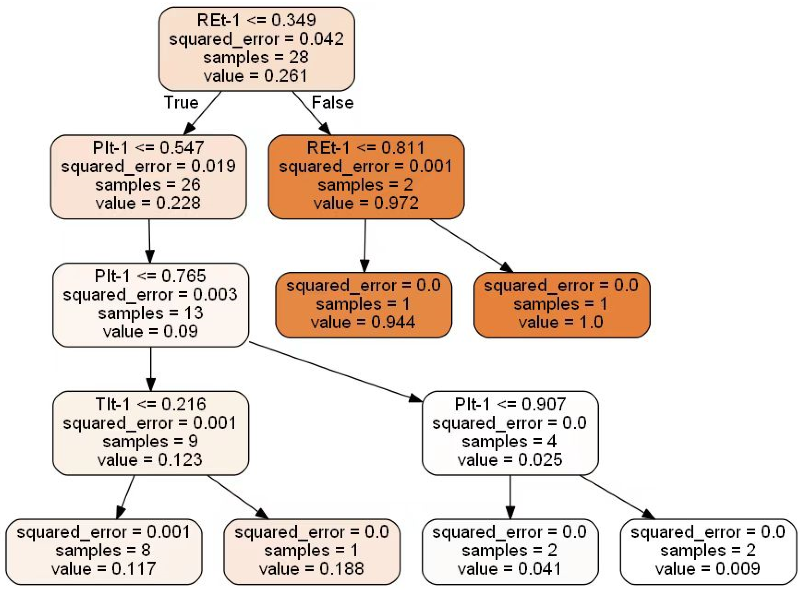
3.2.4. Random Forest (RF)

The RF regression algorithm is a supervised ensemble approach. Multiple random decision trees are generated through random sample and random feature selection [38]. An RF is a collection of uncorrelated decision trees; as such, they generally have a lower variance around their mean.

This study followed four steps to complete the RF regression algorithm:

Step 1: Random re-sampling. A specific number of samples were randomly selected from the training set as the root node samples for each regression tree.

Step 2: Random selection of features. As each regression tree was established, a specific number of candidate features were randomly selected.

Step 3: Construction of decision tree. For the original dataset S, every value (v) of every feature (u) was traversed, and the original dataset S was split into two sets $S_1\left(u,v\right)=\left\{x\right|x_u\le v\}$ and $S_2\left(u,v\right)=\left\{x|x_u>v\right\}$ using the value. The optimal partition feature and partition threshold were identified by solving Formula (8):

$$\begin{array}{c}\underset{u,v}{\min }{\displaystyle \left[\underset{b_1}{\min }{\displaystyle \sum }_{x^{\left(i\right)}\in R_1\left(u,v\right)}{\left(y^{\left(i\right)}-b_1\right)}^2+\underset{b_2}{\min }{\displaystyle \sum }_{x^{\left(i\right)}\in R_2\left(u,v\right)}{\left(y^{\left(i\right)}-b_2\right)}^2\right]}\\ b_i=\mathrm{avg}(y^{\left(i\right)}|x^{\left(i\right)}\in R_i)\end{array}$$

(8)

The above partition was repeated for the two regions until one of the following conditions was met:

(1)

The samples in the children had equal target values.

(2)

The number of samples of nodes reached the threshold.

(3)

The tree reached its maximum depth.

Step 4: RF was used to integrate multiple decision trees. During the prediction process, each decision tree in the RF used test samples as input, and each decision tree returned a prediction result. The RF calculated the average value of these results to generate the prediction output of the test sample.

RF regression includes several decision trees; each is a set of internal nodes and leaves, including split nodes and leaf nodes. A leaf node is a predictive value, and a split node minimizes the sum of the mean square error of the left and right sets obtained after splitting. For each feature, it is necessary to calculate how, on average, the feature decreases the mean square error. The average calculated over all the trees in the forest is the measure of the feature importance.

3.2.5. Gradient Boosting Decision Tree (GBDT)

Boosting algorithm has been proven to have a good prediction effect in small sample scenes [39]. GBDT is composed of regression trees in a series. Each tree learns the residual of the sum of the conclusions of all previous trees. This residual is an accumulated quantity, which is added to the predicted value to generate the true value. Therefore, GBDT can use iterations to train a weak learner to be a strong learner. Assuming L is the loss function, the initial weak learner is expressed as Formula (9):

$$f_0\left(x\right)=\underset{c}{\underbrace{\arg \min }}{\displaystyle \sum }_{i=1}^{m}L\left(y_i,c\right)$$

(9)

Assume that the maximum number of iterations is T, and there are t iteration rounds. The number of iterative steps needed to generate a strong learner from a weak learner is calculated as follows:

(1)

For the sample i = 1, 2, …, m, calculate the negative gradient using Formula (10):

$$r_{ti}=-{\left[\frac{\partial L\left(y_i,f\left(x_i\right)\right)}{\partial f\left(x_i\right)}\right]}_{f\left(x\right)=f_{t-1}\left(x\right)}$$

(10)

Based on $\left(x_i,r_{ti}\right)\left(i=1,2,\dots ,m\right)$, the t-th regression tree is obtained, with a corresponding leaf node region of $R_{tj},j=1,2,\dots ,J$, where J is the number of leaf nodes of regression tree t.

(2)

For the leaf region $j=1,2,\dots ,J$, calculate the best fit value using Formula (11):

$$c_{tj}=\underset{c}{\underbrace{\arg \min }}{\displaystyle \sum }_{x_i\in R_{tj}}L\left(y_i,f_{t-1}\left(x_i\right)+c\right)$$

(11)

(3)

The stronger learner is determined using Formula (12):

$$f_t\left(x\right)=f_{t-1}\left(x\right)+{\displaystyle \sum }_{j=1}^J{c}_{tj}I\left(x\in R_{tj}\right)$$

(12)

Finally, the strong learner is determined using Formula (13):

$$f\left(x\right)=f_T\left(x\right)=f_0\left(x\right)+{\displaystyle \sum }_{t=1}^T{\displaystyle \sum }_{j=1}^J{c}_{tj}I\left(x\in R_{tj}\right)$$

(13)

3.2.6. K-Fold Cross Validation (CV) and Grid Search

Due to the limited data available to predict China’s CO₂ emissions, K-folded CV was used to improve the model’s predictive performance. For this process, CV eliminated independent validation sets. Instead, the whole dataset was divided into five equal parts (K = 5). Each partition, called a fold, served as a validation set. The remaining four folds served as a training set. The technique was repeated five times until each fold had been used as a validation set, with the other four used as a training set. The final accuracy of the model was calculated using the average accuracy of the validation data across the five models. Data from 2010 to 2021 were used as test sets, and the remaining data were divided into training sets and validation sets by CV.

Parameter optimization can effectively improve the accuracy of the model [40]. In this paper, Grid Search (GS) is used to achieve parameter optimization. GS was used to find the optimal parameters. All candidate parameters were adjusted step-by-step, with each possibility tested using a cyclic traversal to identify the parameter with the best-predicted performance. The parameters with the best predicted performance are the final results.

4. Results and Discussion

4.1. Exploratory Data Analysis (EDA)

Using Definition 2 introduced in Section 3.2.1, window sliding widths were denoted as $w\in \left\{1,2,3,4,5,6\right\}$, so six patterns were established to predict China’s short-term CO₂ emissions. The input features of every pattern included renewable energy consumption (RE), the proportion of primary industry (PI), the proportion of secondary industry (SI), and the proportion of tertiary industry (TI). Figure 4 shows the distribution of PI, SI, and TI using box plots. The distribution of SI is the most concentrated and the change is the least. PI has gradually declined, with a rapid decline from the median to the maximum in recent years. On the contrary, TI has gradually increased, with a fast growth rate in recent years.

A correlation analysis was conducted to determine which features were statistically significant with respect to impacts on China’s predicted future CO₂ emissions. Figure 5 shows the Pearson correlation coefficient and P-values for the six patterns. More asterisks indicate a higher level of significance (lower P-value). We found that TI and PI produced high Pearson correlation coefficients and low P-values. There was a significant negative correlation between the proportion of PI and the prediction of CO₂ emissions. Since SI is relatively stable and the variance is small, there was no significant linear correlation between SI and the prediction of CO₂ emissions. When renewable energy consumption increases, carbon emissions per unit of GDP fall. At the present stage in China, carbon emissions still show an increasing trend due to the faster growth of GDP. Therefore, there is a positive correlation between RE and CO₂ emission.

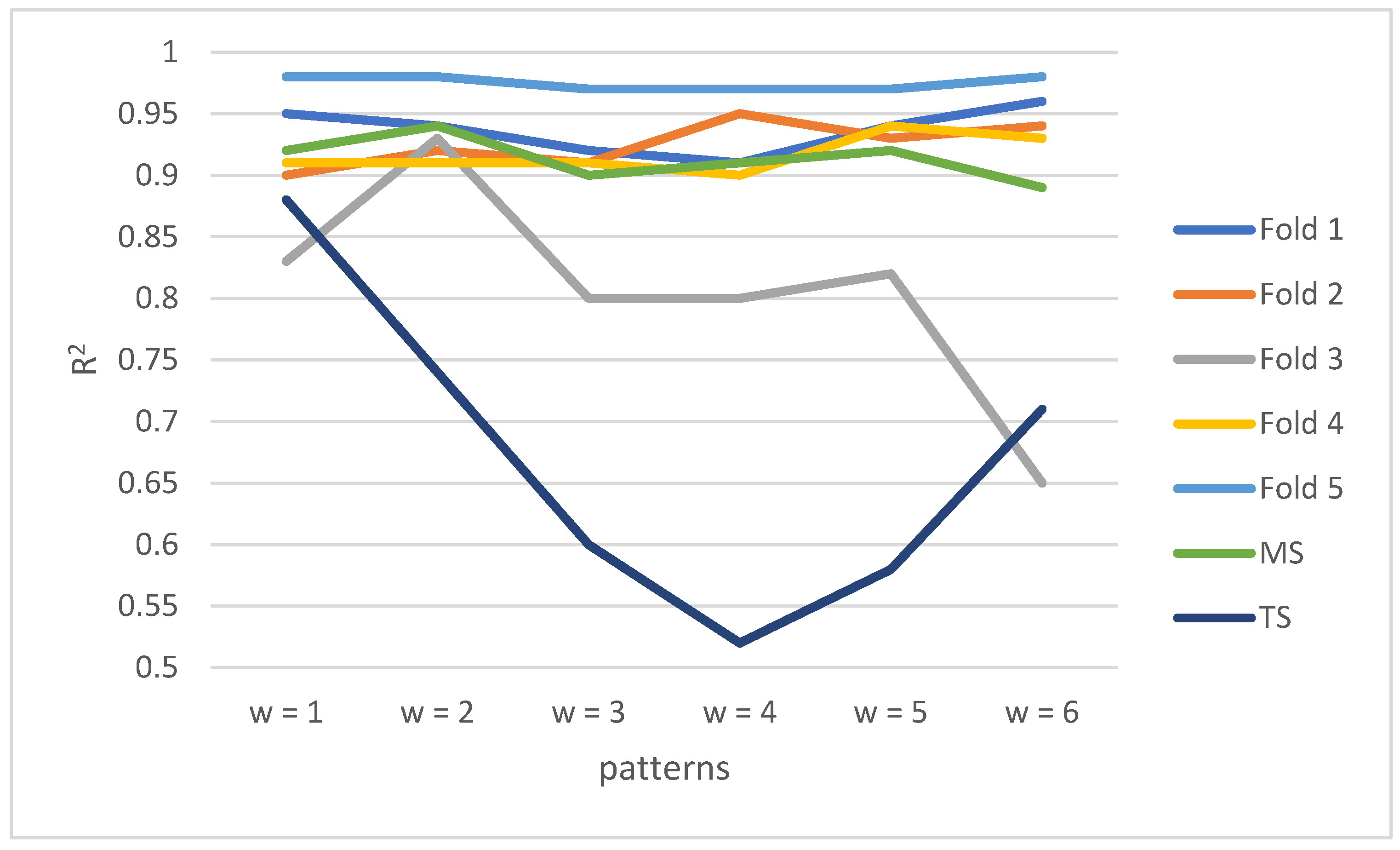
4.2. Cross Validation of Random Forest

The parameters tuned for RF include the maximum number of features (MF), the number of trees (NT), and the maximum depth of trees (MD). MF is expressed as a percentage and is the maximum number of features considered when constructing the optimal model of a decision tree. NT represents the number of sub-datasets generated by sampling with the replacement method. If NT is too small, it is easy for underfitting to occur; if NT is too large, the model performance cannot be significantly improved. During recursive generation, the decision tree constantly aligns to fit the training data, leading to a deepening of the tree depth and improvements in the fitting effect of training data. However, this process may lead to overfitting the training data and poor generalization ability. This highlights the importance of MD as a key parameter.

Table 1. R² of CV and grid search for RF.

	Fold 1	Fold 2	Fold 3	Fold 4	Fold 5	MS	TS	MD	MF	NT
Pattern 1 (w = 1)	0.95	0.9	0.83	0.91	0.98	0.92	0.88	4	0.6	10
Pattern 2 (w = 2)	0.94	0.92	0.93	0.91	0.98	0.94	0.74	4	0.7	10
Pattern 3 (w = 3)	0.92	0.91	0.8	0.91	0.97	0.9	0.6	5	0.7	20
Pattern 4 (w = 4)	0.91	0.95	0.8	0.9	0.97	0.91	0.52	5	0.6	20
Pattern 5 (w = 5)	0.94	0.93	0.82	0.94	0.97	0.92	0.58	3	0.6	10
Pattern 6 (w = 6)	0.96	0.94	0.65	0.93	0.98	0.89	0.71	5	0.8	50

shows the process of cross validation and predicted performances in the test set generated by RF. It shows the optimal parameter combination (MF, NT, MD), the score of each fold, the mean score (MS) in the validation set, and the score in the test dataset (TS). RF had the best prediction performances in the validation set (R² = 0.94) when w = 2 and ranks second in the test set (R² = 0.74). RF has the best prediction performance in the test set (R² = 0.88) when w = 1. RF has the worst prediction performances (R² = 0.89) in the validation set when w = 6; however, the prediction performances (R² = 0.71) in the test set was better compared to the other three patterns. Figure 6 uses a line chart to compare the metrics in the validation set and the test set for RF. The figure shows that pattern 1 returned the best prediction performance in the test set, followed by pattern2 and pattern6.

Figure 7 and Figure 8 show the decision tree growth process. There are 10 decision trees in pattern1. Figure 7 shows the partial growth of one decision tree. A total of 28 samples were randomly resampled from the original sample, and each value of each feature was traversed. RE was selected as the root node, and 0.349 was selected as the optimal segmentation value, because the sum of the mean square error of the samples from the left and right sets was at its minimum at this point (squared_error = 0.042). Figure 7 shows six leaf nodes: Five nodes stopped splitting because the mean square error of the samples contained by them was equal to 0; and the last node stopped splitting due to the restriction of the tree depth.

For Figure 8, a total of 30 samples were randomly resampled from the original sample. The six leaf nodes stopped splitting because the mean square error of the samples contained by them was equal to 0. Three of the six nodes have only one sample remaining, and three nodes reach the maximum depth of the tree.

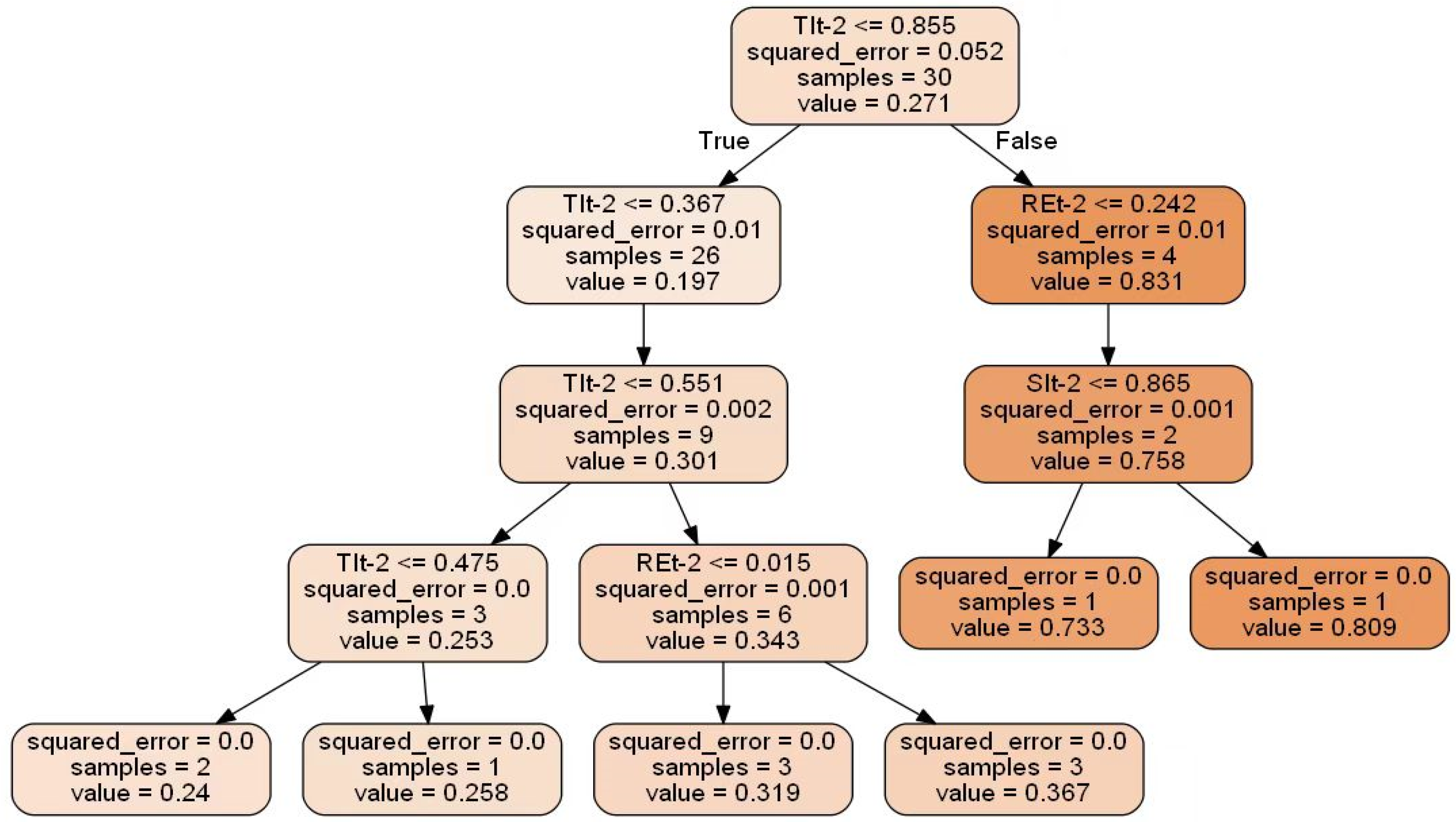
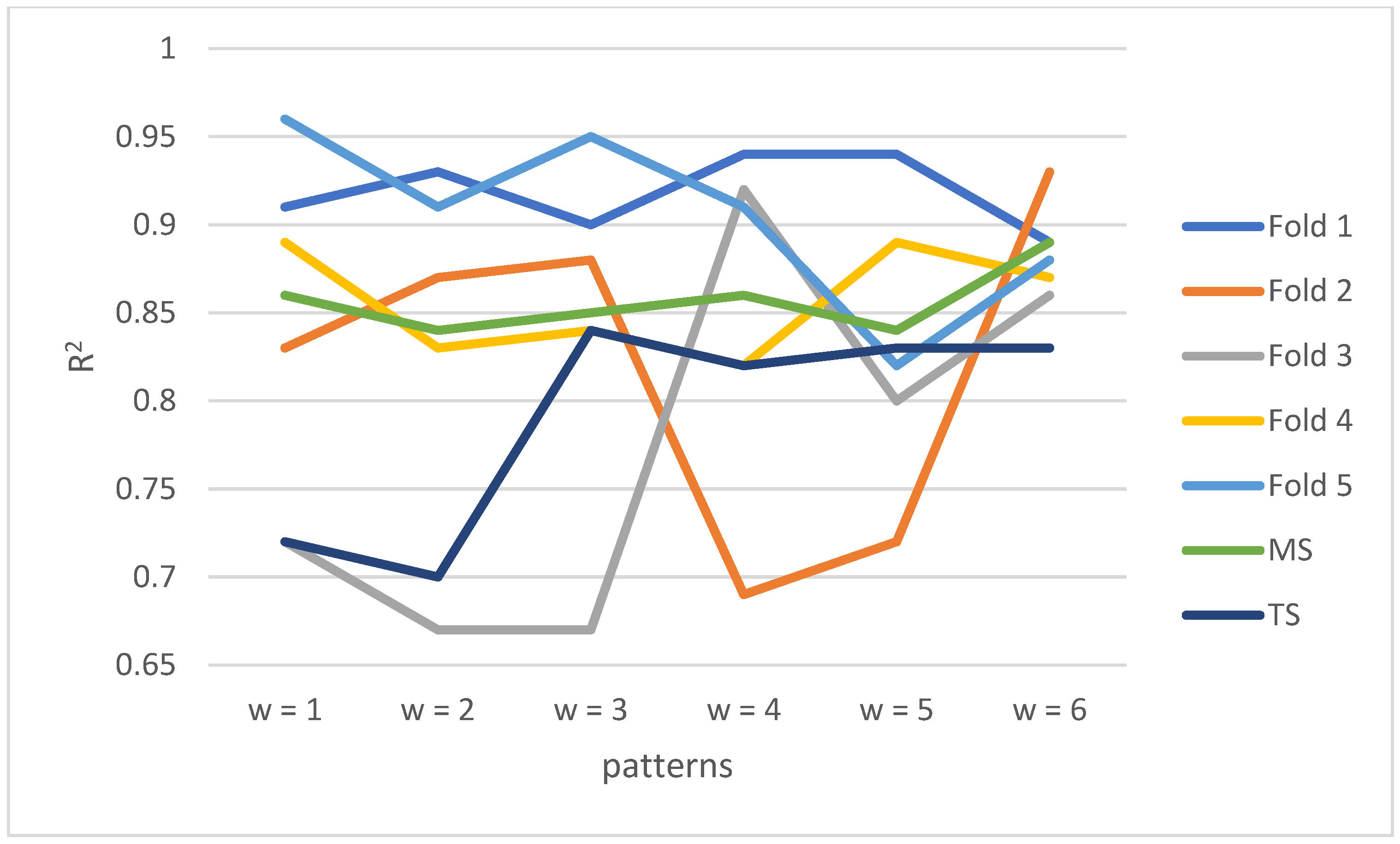
4.3. Cross Validation of LASSO

Table 2. R² of Cross validation and grid search of LASSO.

	Fold 1	Fold 2	Fold 3	Fold 4	Fold 5	MS	TS	Alpha
w = 1	0.91	0.83	0.72	0.89	0.96	0.86	0.72	0.0023
w = 2	0.93	0.87	0.67	0.83	0.91	0.84	0.7	0.0021
w = 3	0.9	0.88	0.67	0.84	0.95	0.85	0.84	0.00057
w = 4	0.94	0.69	0.92	0.82	0.91	0.86	0.82	0.00189
w = 5	0.94	0.72	0.8	0.89	0.82	0.84	0.83	0.00002
w = 6	0.89	0.93	0.86	0.87	0.88	0.89	0.83	0.003

shows the process of cross validation and predicted performances in the test set using LASSO. It shows the parameter (alpha), the score of each fold, the mean score (MS) in the validation set of each pattern; and the score in the test set (TS). LASSO resulted in the best fitting effect in the validation set (R² = 0.89) when w = 6 and had the second-highest prediction performances in the test set (R² = 0.83). LASSO had the best prediction performance in the test set (R² = 0.84) when w = 3. LASSO’s prediction performances in the test set was worse when w = 1 and w = 2 than other patterns.

Figure 9 displays a line chart to compare CV and prediction metrics using LASSO. The figure shows that pattern 3 had the best prediction performance in the test set, followed by pattern 5, pattern 6 and pattern 4. The prediction score of LASSO in the test set is lower than that in the validation set, which means that LASSO overfits in the validation set and is not robust enough for data distribution.

4.4. Model Selection

Table 3. Comparative assessment of shallow learning models in the test set.

	SVR		Ridge		LASSO		RF		GBDT		RF-LASSO
	R2	RMSE	R2	RMSE	R2	RMSE	R2	RMSE	R2	RMSE	R2	RMSE
w = 1	0.80	0.14	0.67	0.17	0.72	0.16	0.88	0.10	0.79	0.14	0.88	0.10
w = 2	0.67	0.17	0.56	0.20	0.70	0.16	0.74	0.15	0.37	0.24	0.74	0.15
w = 3	0.75	0.15	0.67	0.17	0.84	0.12	0.60	0.19	0.32	0.25	0.84	0.12
w = 4	0.76	0.15	0.66	0.17	0.82	0.13	0.52	0.21	0.29	0.25	0.82	0.13
w = 5	0.79	0.14	0.69	0.17	0.83	0.12	0.58	0.2	0.35	0.24	0.83	0.12
w = 6	0.82	0.13	0.72	0.16	0.83	0.12	0.71	0.16	0.67	0.17	0.83	0.12
mean	0.77	0.15	0.66	0.17	0.79	0.14	0.67	0.17	0.47	0.22	0.82	0.12

presents the prediction performances from the testing set for China’s short-term CO₂ emissions. The results confirm that RF-LASSO performed best among all ML models, and LASSO and SVR ranked second and third for prediction performance, respectively. The predicted scores in the test set of RF-LASSO and LASSO all exceeded 0.70 for different values of w. However, the score of SVR was poor (R² = 0.67) when w = 2.

Figure 10 shows two radar diagrams and one box diagram to compare the prediction performance of all ML models in the test set. The radar plots showing R² and RMSE are reversed. For R², the line describing GBDT clearly remained in the innermost layer. This indicates that GBDT had the poorest predicted effect on short-term CO₂ emissions. The prediction performance of the RF was the optimal significantly at w = 1 and w = 2. The Mean Absolute Error (MAE) is the average absolute error between predicted and observed values. The box diagram in Figure 10 shows the MAE generated by all models when predicting short-term CO₂ emissions. RF-LASSO had the smallest MAE, followed by LASSO and SVR. Ridge had the best stability, followed by RF-LASSO, SVR, and LASSO.

Ridge and LASSO are linear regression regularization methods, both of which can solve the multicollinearity problem in multiple linear regressions and enhance the stability of the model. In this study, LASSO set the coefficient of SI to 0, which made the model more explanatory, while Ridge could only reduce the coefficient of SI close to 0. Since SI is basically stable, LASSO compresses the coefficient of SI to 0, resulting in a higher prediction score of the model in the test set.

4.5. Future Carbon Dioxide Emissions

This study uses the sliding window method to transform a time-series prediction into a supervised learning problem, so that historical data can be used to predict future carbon dioxide emissions in China. The models obtained with six window widths can predict carbon dioxide emissions in different time periods in the future, as shown in Figure 11. The sample data from 2011 to 2021 is a test set divided separately from the dataset, which were not seen by the model during the training process.

The prediction results of the six models in the test set fluctuate slightly around the labels. For the prediction of future carbon dioxide emissions, the model with a window width of 6 can predict carbon emissions in the next six years, and the carbon emissions can be obtained for as far as 2027. The prediction results of the six models for future carbon emissions are consistent with the overall trend. Although there is a short decline period, the development trend of carbon dioxide emissions is still growing. Although the rate of increase in CO2 emissions slow significantly since 2024, carbon dioxide emissions will reach 10.3 billion tons by 2027. It can be seen that the task of China to achieve its carbon peak on schedule is very heavy.

4.6. Feature Importance

RF and LASSO are interpretable. For time-series data, the features that are important for the CO₂ emissions prediction should not only be closely related to labels, but also have volatility. Figure 12 was generated using the mean value of the feature importance score using RF-LASSO in different patterns. RE was the most important for China’s CO₂ emissions prediction and its importance significantly fluctuated.

PI and TI rank as the second and third most important factors in CO₂ emissions prediction, mainly because the overall proportion of the primary industry is decreasing and the proportion of the tertiary industry is increasing. The tertiary industry has gradually become the main contributor to China’s incremental CO₂ emissions. Despite the fact that CO₂ emissions from the secondary industry consistently make up a large proportion of total CO₂ emissions, the change in SI is small, making it a less important factor in prediction. Therefore, the adjustment of industrial structure is very important for forecasting China’s carbon dioxide emissions.

The results of the feature importance analysis show that renewable energy consumption and industrial structure are closely related to China’s carbon dioxide emissions. Under the “double carbon” target, China has taken measures from two aspects to effectively curb the growth rate of carbon emissions: On the one hand, increase the consumption of renewable energy and reduce the proportion of fossil energy consumption, so as to optimize the energy structure; on the other hand, it is committed to building a modern industrial system with high-tech industry as the lead, service economy as the main body, advanced manufacturing as the support, and modern agriculture as the basis. Over the past decade, China’s carbon emission intensity has dropped by 34.4 percent, reversing the trend of rapid growth in carbon dioxide emissions. As a result, the increase in renewable energy consumption and the optimization of the industrial structure have positive impacts on curbing carbon dioxide emissions.

5. Conclusions

This study applied different shallow ML models to predict China’s short-term CO₂ emissions using historical data in China. Input data included the share of primary, secondary, and tertiary industries and renewable energy consumption for the period of 1965 to 2021. Different sliding window widths were used to transform time-series predictions into supervised learning problems, with six design patterns.

The key findings of this study are summarized as follows. (1) The combined model of RF and LASSO performed the best in predicting China’s short-term CO₂ emissions, followed by LASSO and SVR. The prediction performance of RF was very fragile to the window width. Specifically, the prediction effect of RF on CO₂ emission varied significantly for different time windows. GBDT had the worst prediction performances among all the models. (2) The sliding window method is used to convert time-series predictions into supervision problems, and historical data can be used to predict future carbon dioxide emissions. To ensure that the feature data are real, the model can predict CO₂ emissions for up to six years ahead. (3) Cross validation and a grid search were critical for optimizing China’s CO₂ emissions prediction with small datasets. (4) By 2027, carbon dioxide emissions will continue to grow and reach 10.3 billion tons. It can be seen that the task of China to achieve its carbon peak on schedule is very heavy. (5) According to the feature importance analysis, renewable energy consumption is most important for CO₂ emissions prediction, followed by the proportion of primary and tertiary industries.

This study concludes that increases in renewable energy consumption and adjustments to the industrial structure have played an important role in curbing China’s CO₂ emissions. To achieve strategic goals related to carbon peaking and carbon neutrality, the energy structure and industrial structure need to be further optimized. This could include accelerating the shift from fossil energy to renewable energy, reducing the proportion of energy-intensive industries, and increasing the proportion of high-tech industries.

This study demonstrated that shallow learning can achieve good results in developing short-term predictions of China’s CO₂ emissions based on historical characteristics. Future research should focus on the following aspects: (1) Analyzing the impact of other characteristics on China’s predicted CO₂ emissions (i.e., energy consumption structure, urbanization level); (2) in the process of converting time-series data into supervised data with labels, constructing different patterns to predict CO₂ emissions; and (3) from a technical perspective, using stacking models to further improve CO₂ emission predictions.

References

1. Inergovernmental Panel on Climate Change (IPCC). Contribution of Working Group III to the Sixth Assessment Report of the Intergovernmental Panel on Climate Change; Shukla, P.R., Skea, J., Slade, R., Al Khourdajie, A., van Diemen, R., McCollum, D., Pathak, M., Some, S., Vyas, P., Fradera, R., et al., Eds.; Cambridge University Press: Cambridge, UK, 2022. [Google Scholar]
2. Song, M.; Zhu, S.; Wang, J.; Zhao, J. Share green growth: Regional evaluation of green output performance in China. Int. J. Prod. Econ. 2020, 219, 152–163. [Google Scholar] [CrossRef]
3. Wang, W.W.; Zhang, M.; Zhou, M. Using LMDI method to analyze transport sector CO2 emissions in China. Energy 2011, 36, 5909–5915. [Google Scholar] [CrossRef]
4. Jing, Q.; Bai, H.; Luo, W.; Cai, B.; Xu, H. A top-bottom method for city-scale energy-related CO2 emissions estimation: A case study of 41 Chinese cities. J. Clean. Prod. 2018, 202, 444–455. [Google Scholar] [CrossRef]
5. Wang, H.; Chen, Z.; Wu, X.; Nie, X. Can a carbon trading system promote the transformation of a low-carbon economy under the framework of the porter hypothesis?—Empirical analysis based on the PSM-DID method. Energy Policy 2019, 129, 930–938. [Google Scholar] [CrossRef]
6. Ma, X.; Wang, C.; Dong, B.; Gu, G.; Chen, R.; Li, Y.; Zou, H.; Zhang, W.; Li, Q. Carbon emissions from energy consumption in China: Its measurement and driving factors. Sci. Total Environ. 2019, 648, 1411–1420. [Google Scholar] [CrossRef]
7. Wang, M.; Feng, C. Using an extended logarithmic mean Divisia index approach to assess the roles of economic factors on industrial CO2 emissions of China. Energy Econ. 2018, 76, 101–114. [Google Scholar] [CrossRef]
8. Abokyi, E.; Appiah-Konadu, P.; Tangato, K.F.; Abokyi, F. Electricity consumption and carbon dioxide emissions: The role of trade openness and manufacturing sub-sector output in Ghana. Energy Clim. Chang. 2021, 2, 100026. [Google Scholar] [CrossRef]
9. Hou, J.; Hou, P. Polarization of CO2 emissions in China’s electricity sector: Production versus consumption perspectives. J. Clean. Prod. 2018, 178, 384–397. [Google Scholar] [CrossRef]
10. Lin, B.; Tan, R. Sustainable development of China’s energy intensive industries: From the aspect of carbon dioxide emissions reduction. Renew. Sustain. Energy Rev. 2017, 77, 386–394. [Google Scholar] [CrossRef]
11. Zhang, X.; Wang, F. Hybrid input-output analysis for life-cycle energy consumption and carbon emissions of China’s building sector. Build. Environ. 2016, 104, 188–197. [Google Scholar] [CrossRef]
12. Zhang, Z.; Wang, B. Research on the life-cycle CO2 emission of China’s construction sector. Energy Build. 2016, 112, 244–255. [Google Scholar] [CrossRef]
13. Du, Z.; Lin, B. Changes in automobile energy consumption during urbanization: Evidence from 279 cities in China. Energy Policy 2019, 132, 309–317. [Google Scholar] [CrossRef]
14. Zhao, M.; Sun, T. Dynamic spatial spillover effect of new energy vehicle industry policies on carbon emission of transportation sector in China. Energy Policy 2022, 165, 112991. [Google Scholar] [CrossRef]
15. Guan, D.; Hubacek, K.; Weber, C.L.; Peters, G.P.; Reiner, D.M. The drivers of Chinese CO2 emissions from 1980 to 2030. Glob. Environ. Chang. 2008, 18, 626–634. [Google Scholar] [CrossRef] [Green Version]
16. Fan, J.-L.; Da, Y.-B.; Wan, S.-L.; Zhang, M.; Cao, Z.; Wang, Y.; Zhang, X. Determinants of carbon emissions in ‘Belt and Road initiative’ countries: A production technology perspective. Appl. Energy 2019, 239, 268–279. [Google Scholar] [CrossRef]
17. Net, X. Statement by H.E. Xi Jinping President of the People’s Republic of China At the General Debate of the 75th Session of The United Nations General Assembly. Available online: https://baijiahao.baidu.com/s?id=1678546728556033497&wfr=spider&for=pc (accessed on 25 June 2022).
18. Xiong, P.P.; Xiao, L.S.; Liu, Y.C.; Yang, Z.; Zhou, Y.F.; Cao, S.R. Forecasting carbon emissions using a multi-variable GM (1,N) model based on linear time-varying parameters. J. Intell. Fuzzy Syst. 2021, 41, 6137–6148. [Google Scholar] [CrossRef]
19. Ye, L.; Yang, D.L.; Dang, Y.G.; Wang, J.J. An enhanced multivariable dynamic time-delay discrete grey forecasting model for predicting China’s carbon emissions. Energy 2022, 249, 123681. [Google Scholar] [CrossRef]
20. Zhang, F.; Deng, X.Z.; Xie, L.; Xu, N. China’s energy-related carbon emissions projections for the shared socioeconomic pathways. Resour. Conserv. Recycl. 2021, 168, 105456. [Google Scholar] [CrossRef]
21. Li, B.; Han, S.W.; Wang, Y.F.; Li, J.Y.; Wang, Y. Feasibility assessment of the carbon emissions peak in China’s construction industry: Factor decomposition and peak forecast. Sci. Total Environ. 2020, 706, 135716. [Google Scholar] [CrossRef]
22. Zheng, J.L.; Mi, Z.F.; Coffman, D.; Milcheva, S.; Shan, Y.L.; Guan, D.B.; Wang, S.Y. Regional development and carbon emissions in China. Energy Econ. 2019, 81, 25–36. [Google Scholar] [CrossRef]
23. Dong, B.Y.; Ma, X.J.; Zhang, Z.L.; Zhang, H.B.; Chen, R.M.; Song, Y.Q.; Shen, M.C.; Xiang, R.B. Carbon emissions, the industrial structure and economic growth: Evidence from heterogeneous industries in China. Environ. Pollut. 2020, 262, 114322. [Google Scholar] [CrossRef] [PubMed]
24. Siqin, Z.Y.; Niu, D.X.; Li, M.Y.; Zhen, H.; Yang, X.L. Carbon dioxide emissions, urbanization level, and industrial structure: Empirical evidence from North China. Environ. Sci. Pollut. Res. 2022, 29, 34528–34545. [Google Scholar] [CrossRef] [PubMed]
25. Dong, K.Y.; Sun, R.J.; Hochman, G. Do natural gas and renewable energy consumption lead to less CO2 emission? Empirical evidence from a panel of BRICS countries. Energy 2017, 141, 1466–1478. [Google Scholar] [CrossRef]
26. Zheng, H.Y.; Song, M.L.; Shen, Z.Y. The evolution of renewable energy and its impact on carbon reduction in China. Energy 2021, 237, 121639. [Google Scholar] [CrossRef]
27. Abbasi, K.R.; Shahbaz, M.; Zhang, J.J.; Irfan, M.; Alvarado, R. Analyze the environmental sustainability factors of China: The role of fossil fuel energy and renewable energy. Renew. Energy 2022, 187, 390–402. [Google Scholar] [CrossRef]
28. Sun, W.; Ren, C.M. Short-term prediction of carbon emissions based on the EEMD-PSOBP model. Environ. Sci. Pollut. Res. 2021, 28, 56580–56594. [Google Scholar] [CrossRef]
29. Shi, M.S. Forecast of China’s carbon emissions under the background of carbon neutrality. Environ. Sci. Pollut. Res. 2022, 29, 43019–43033. [Google Scholar] [CrossRef]
30. Zhang, J.X.; Zhang, H.; Wang, R.; Zhang, M.X.; Huang, Y.Z.; Hu, J.H.; Peng, J.Y. Measuring the critical influence factors for predicting carbon dioxide emissions of expanding megacities by XGBoost. Atmosphere 2022, 13, 599. [Google Scholar] [CrossRef]
31. Lu, X.Y.; Ota, K.R.; Dong, M.X.; Yu, C.; Jin, H. Predicting transportation carbon emission with urban big data. IEEE Trans. Sustain. Comput. 2017, 2, 333–344. [Google Scholar] [CrossRef] [Green Version]
32. Ning, L.Q.; Pei, L.J.; Li, F. Forecast of China’s carbon emissions based on ARIMA method. Discret. Dyn. Nat. Soc. 2021, 2021, 1441942. [Google Scholar] [CrossRef]
33. Magazzino, C.; Mele, M.; Schneider, N. A machine learning approach on the relationship among solar and wind energy production, coal consumption, GDP, and CO2 emissions. Renew. Energy 2021, 167, 99–115. [Google Scholar] [CrossRef]
34. Ahmed, M.; Shuai, C.M.; Ahmed, M. Influencing factors of carbon emissions and their trends in China and India: A machine learning method. Environ. Sci. Pollut. Res. 2022, 29, 48424–48437. [Google Scholar] [CrossRef]
35. Ullah, I.; Liu, K.; Yamamoto, T.; Al Mamlook, R.E.; Jamal, A. A comparative performance of machine learning algorithm to predict electric vehicles energy consumption: A path towards sustainability. Energy Environ. 2021. [Google Scholar] [CrossRef]
36. Cortes, C.; Vapnik, V. Support-vector networks. Mach. Learn. 1995, 20, 273–297. [Google Scholar] [CrossRef]
37. Hamrani, A.; Akbarzadeh, A.; Madramootoo, C.A. Machine learning for predicting greenhouse gas emissions from agricultural soils. Sci. Total Environ. 2020, 741, 140338. [Google Scholar] [CrossRef]
38. Breiman, L. Random forests. Mach. Learn. 2001, 45, 5–32. [Google Scholar] [CrossRef] [Green Version]
39. Ullah, I.; Liu, K.; Yamamoto, T.; Zahid, M.; Jamal, A. Prediction of electric vehicle charging duration time using ensemble machine learning algorithm and Shapley additive explanations. Int. J. Energy Res. 2022, 46, 15211–15230. [Google Scholar] [CrossRef]
40. Ullah, I.; Liu, K.; Yamamoto, T.; Shafiullah, M.; Jamal, A. Grey wolf optimizer-based machine learning algorithm to predict electric vehicle charging duration time. Transp. Lett. Int. J. Transp. Res. 2022. [Google Scholar] [CrossRef]
Figure 1. Carbon dioxide emissions in China.
Energies 15 08642 g001
Figure 2. The proportion of primary, secondary, and tertiary industries.
Energies 15 08642 g002
Figure 3. Renewable energy consumption in China.
Energies 15 08642 g003
Figure 4. Distribution of PI, SI and TI. ◆ indicates an outlier.
Energies 15 08642 g004
Figure 5. Pearson correlation coefficient of CO2 emissions and input variables for six window widths. *, ** and *** reflect the significant level of 5%, 1% and 0.1%.
Energies 15 08642 g005
Figure 6. Metrics comparison in the validation set and the test set for RF.
Energies 15 08642 g006
Figure 7. Decision tree generation in pattern 1.
Energies 15 08642 g007
Figure 8. Decision tree generation in pattern 2.
Energies 15 08642 g008
Figure 9. Metrics comparison in the validation set and the test set for LASSO.
Energies 15 08642 g009
Figure 10. Comparative assessment of shallow learning models in the testing set.
Energies 15 08642 g010aEnergies 15 08642 g010b
Figure 11. Predicting future carbon dioxide emissions for six window widths.
Energies 15 08642 g011
Figure 12. Feature importance of RF-LASSO.
Energies 15 08642 g012