Author Contributions
Conceptualization, J.C.P. and M.L.S.A.; methodology, J.C.P. and M.L.S.A.; software, J.C.P. and P.H.T.B.; validation, J.C.P. and P.H.T.B.; formal analysis, J.C.P., P.H.T.B. and M.L.S.A.; investigation, J.C.P.; resources, J.C.P.; data curation, J.C.P.; writing—original draft preparation, J.C.P.; writing—review and editing, J.C.P., P.H.T.B. and M.L.S.A.; visualization, J.C.P. and M.L.S.A.; supervision, revision and verifying the results, J.C.P., P.H.T.B. and M.L.S.A. All authors have read and agreed to the published version of the manuscript.
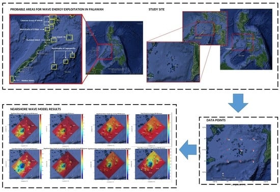
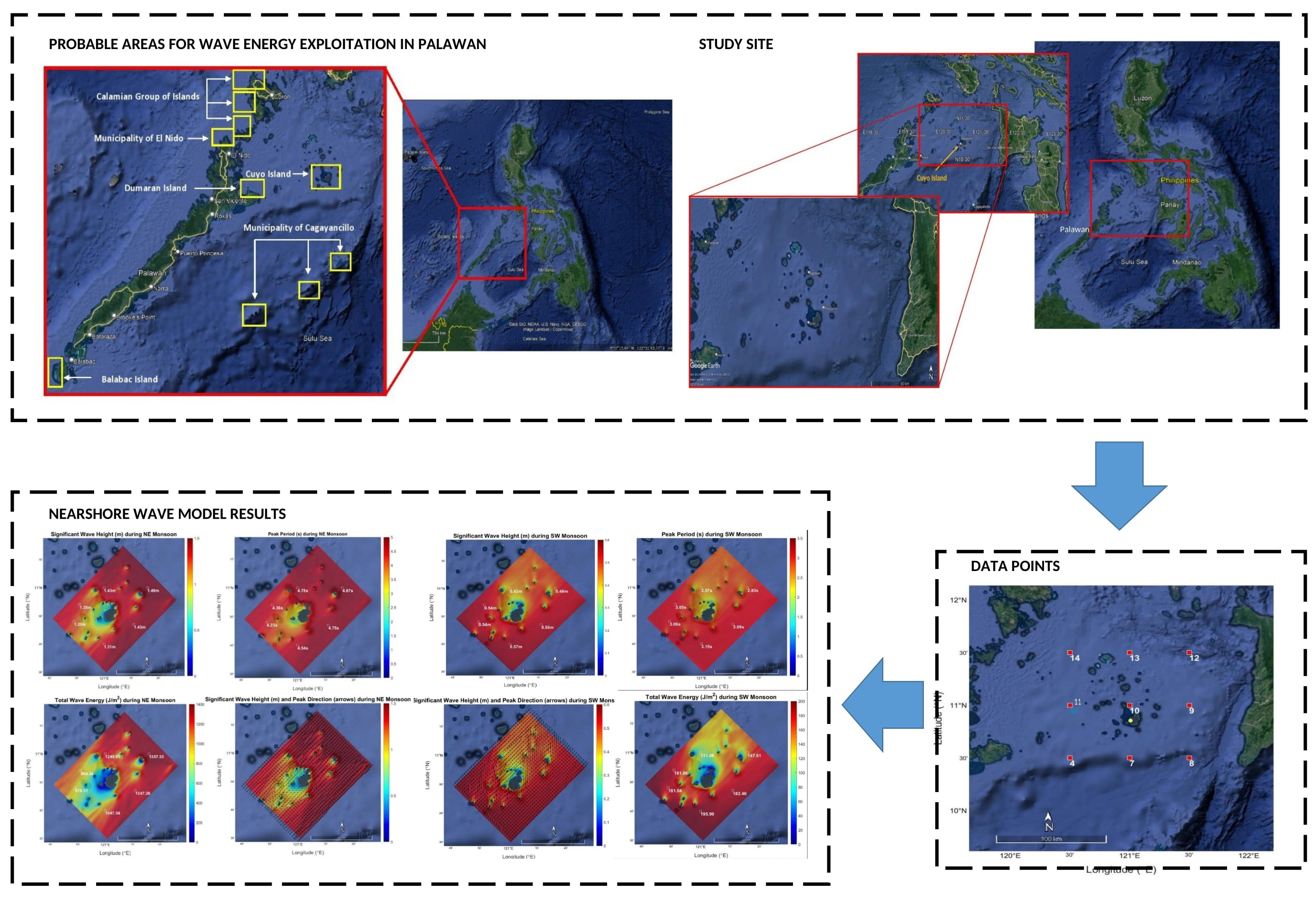
Figure 1.
Probable sites for wave energy development (yellow boxes) in the province of Palawan identified by University of the Philippines’ Marine Science Institute.
Figure 1.
Probable sites for wave energy development (yellow boxes) in the province of Palawan identified by University of the Philippines’ Marine Science Institute.
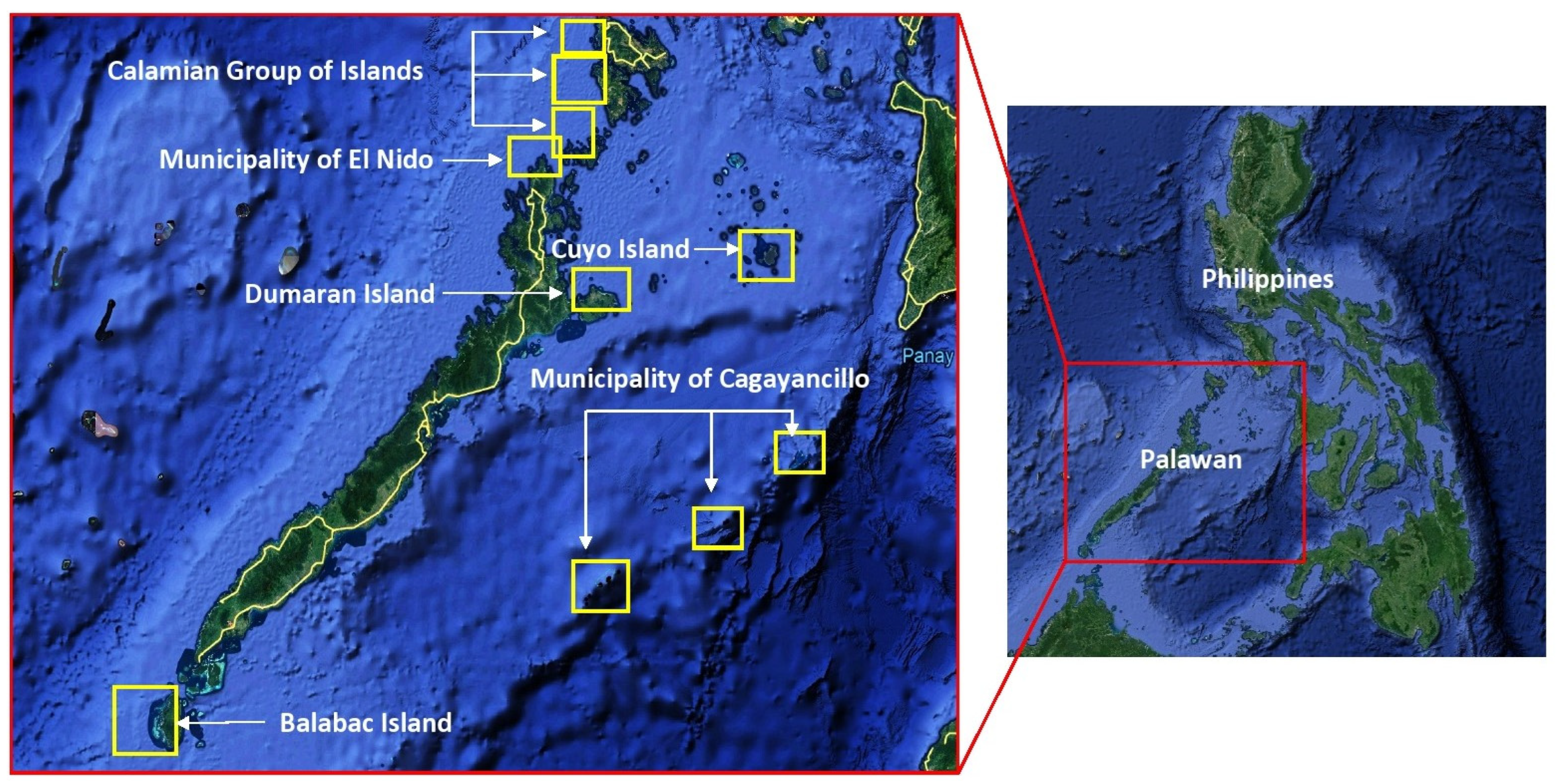
Figure 2.
Map showing the study site, Cuyo Island at the northeastern part of Palawan.
Figure 2.
Map showing the study site, Cuyo Island at the northeastern part of Palawan.
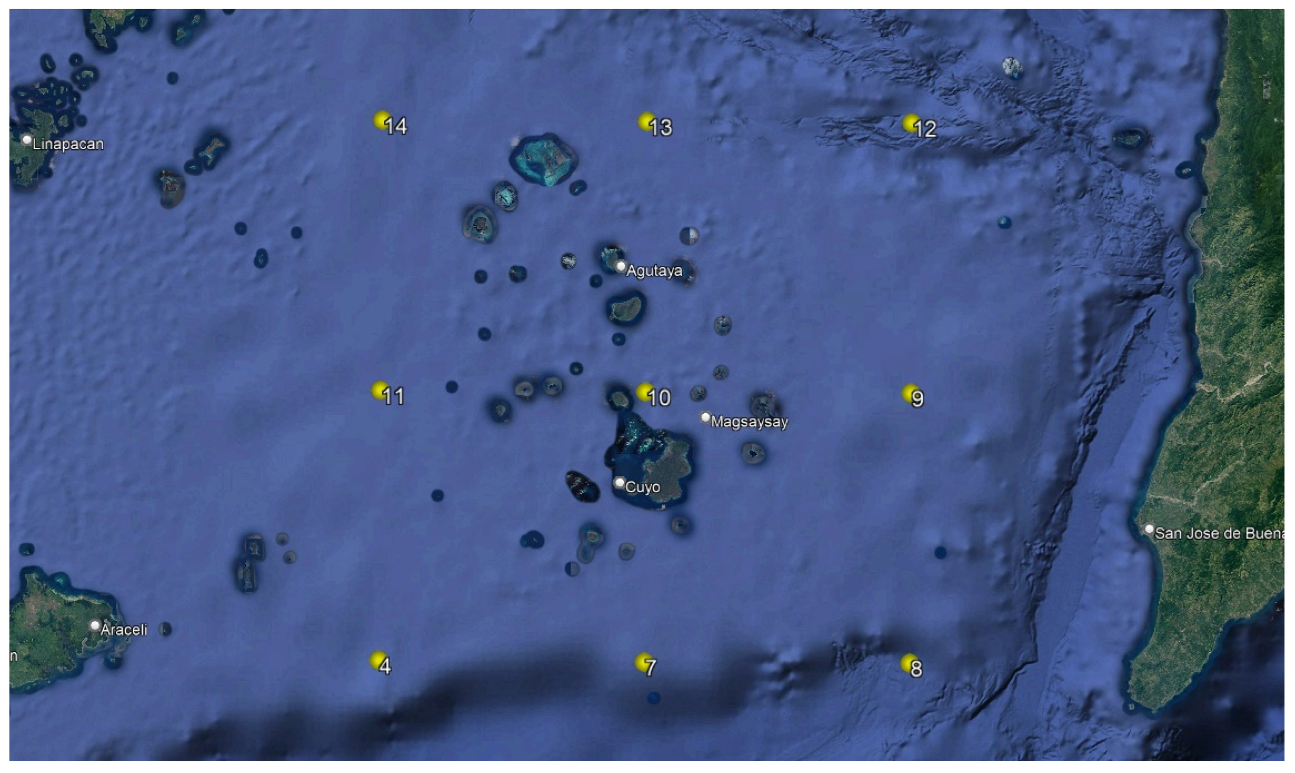
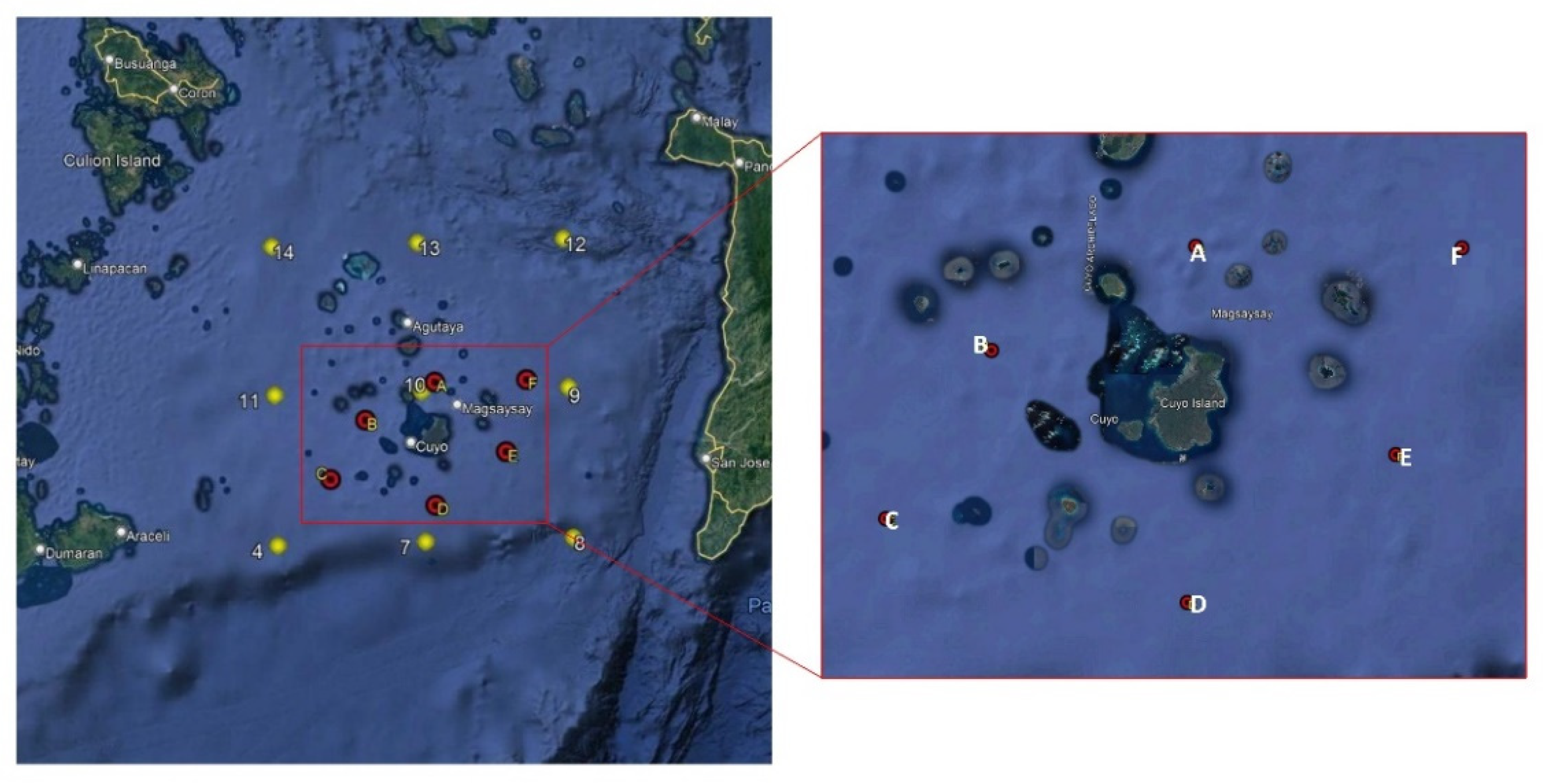
Figure 3.
Cuyo Island showing the 9 stations of MOV’s 40-year hindcast wave data used to determine the average Pd and Hs surrounding Cuyo Archipelago (yellow dots) and used as initial conditions to SWAN (stations 4, 8, 12 and 14).
Figure 3.
Cuyo Island showing the 9 stations of MOV’s 40-year hindcast wave data used to determine the average Pd and Hs surrounding Cuyo Archipelago (yellow dots) and used as initial conditions to SWAN (stations 4, 8, 12 and 14).
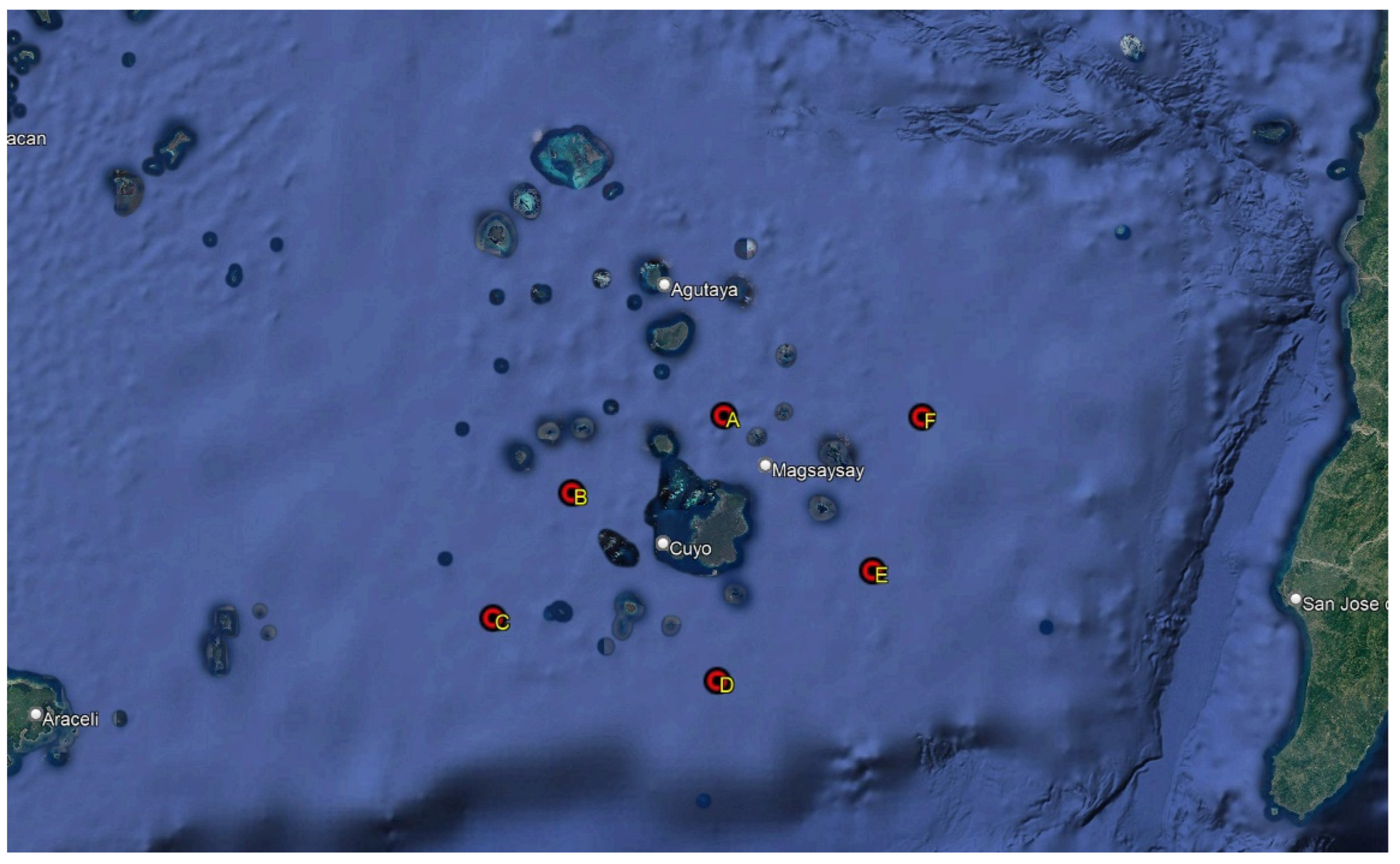
Figure 4.
Chosen sites of interest (stations A–F) about 23 km from PAGASA station used to match with WEC to determine the potential annual energy production surrounding the island.
Figure 4.
Chosen sites of interest (stations A–F) about 23 km from PAGASA station used to match with WEC to determine the potential annual energy production surrounding the island.
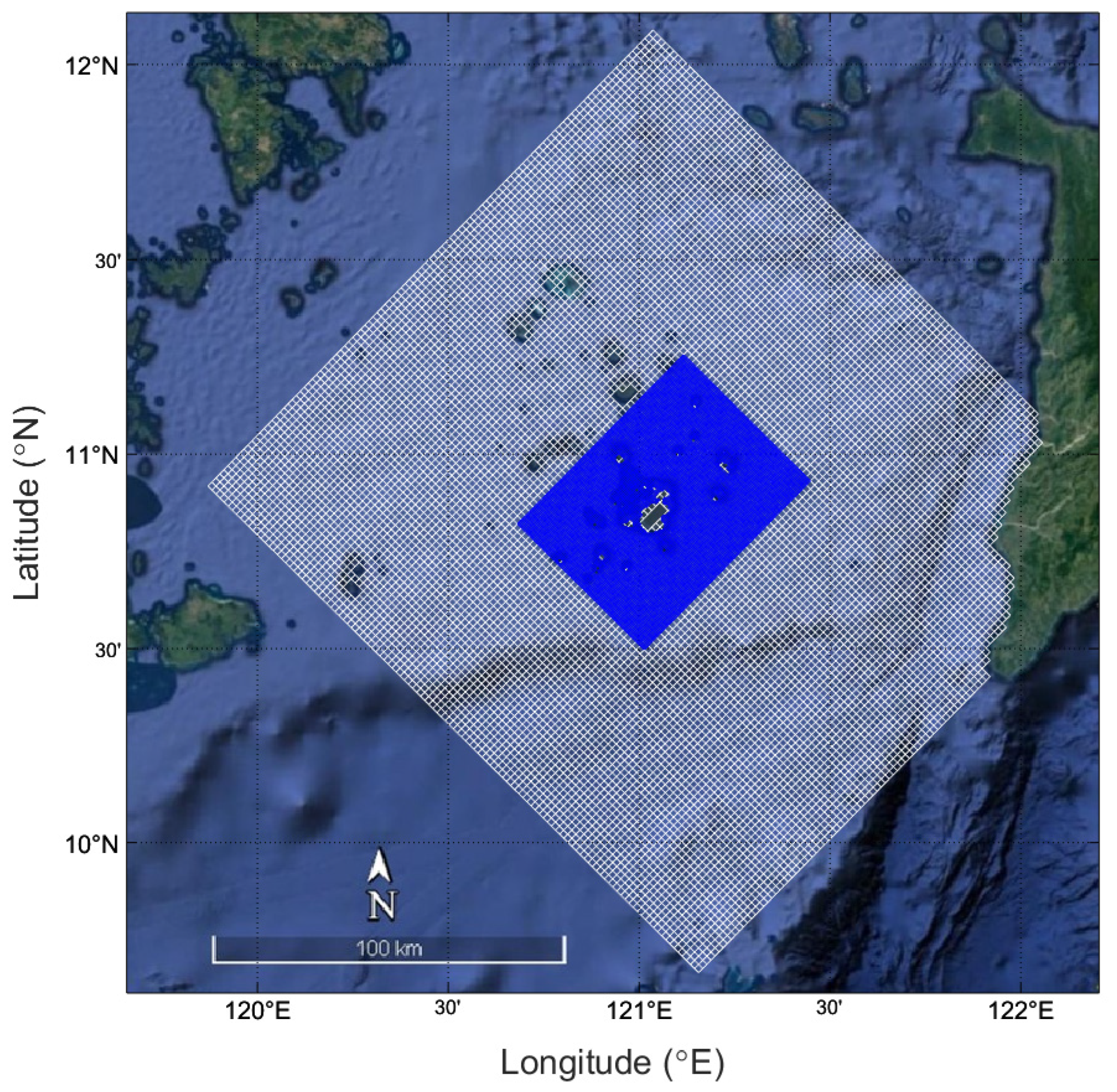
Figure 5.
Nested grids (white for coarse grid, 110 × 120 with ~150 km resolution; blue for fine grid, 123 × 93 with ~500 m resolution) used for the SWAN modelling.
Figure 5.
Nested grids (white for coarse grid, 110 × 120 with ~150 km resolution; blue for fine grid, 123 × 93 with ~500 m resolution) used for the SWAN modelling.
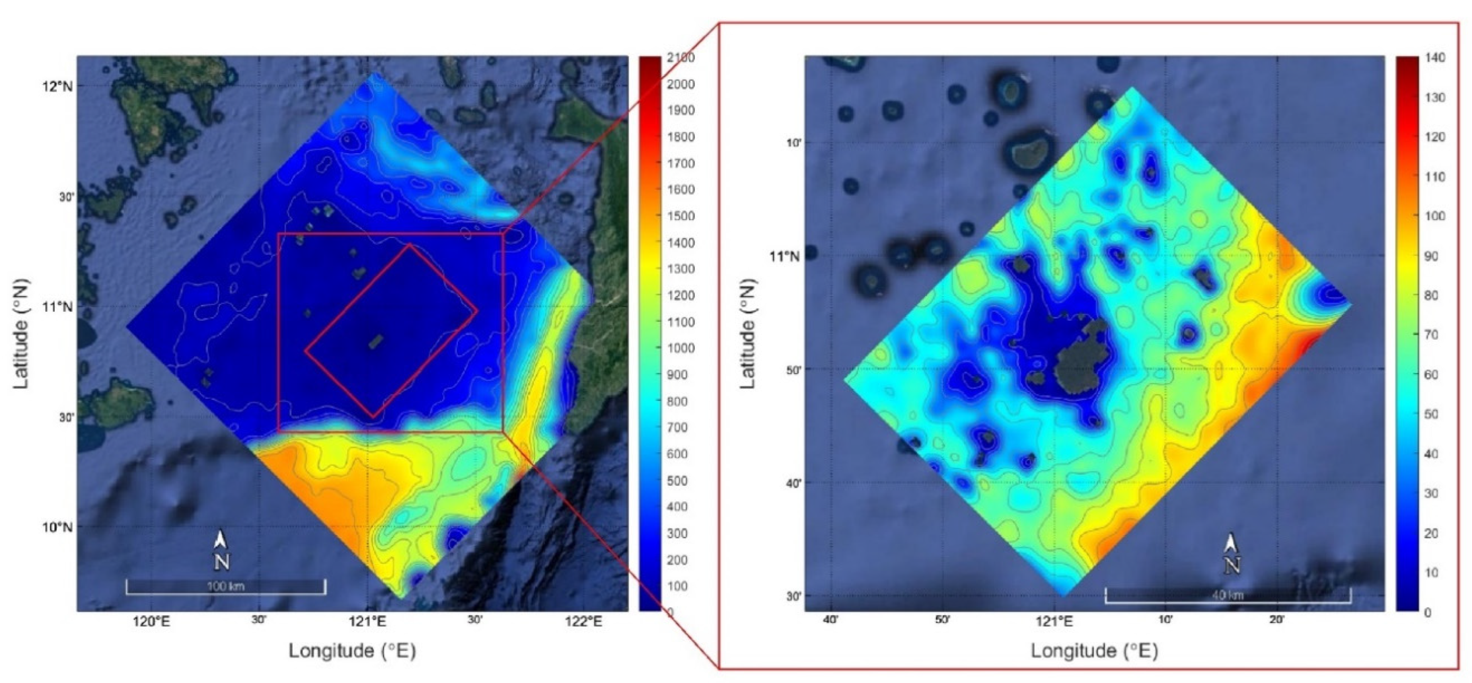
Figure 6.
Downloaded GEBCO bathymetric data (adjusted to positive values in meters for Delft3d compatibility) interpolated onto the coarse (left panel) and fine (right panel) grid of the SWAN model. Red is deepest and blue is shallowest. Contour intervals for coarse grid (left panel) are every 100 m depth, while it is every 10 m of depth for fine grid (right panel).
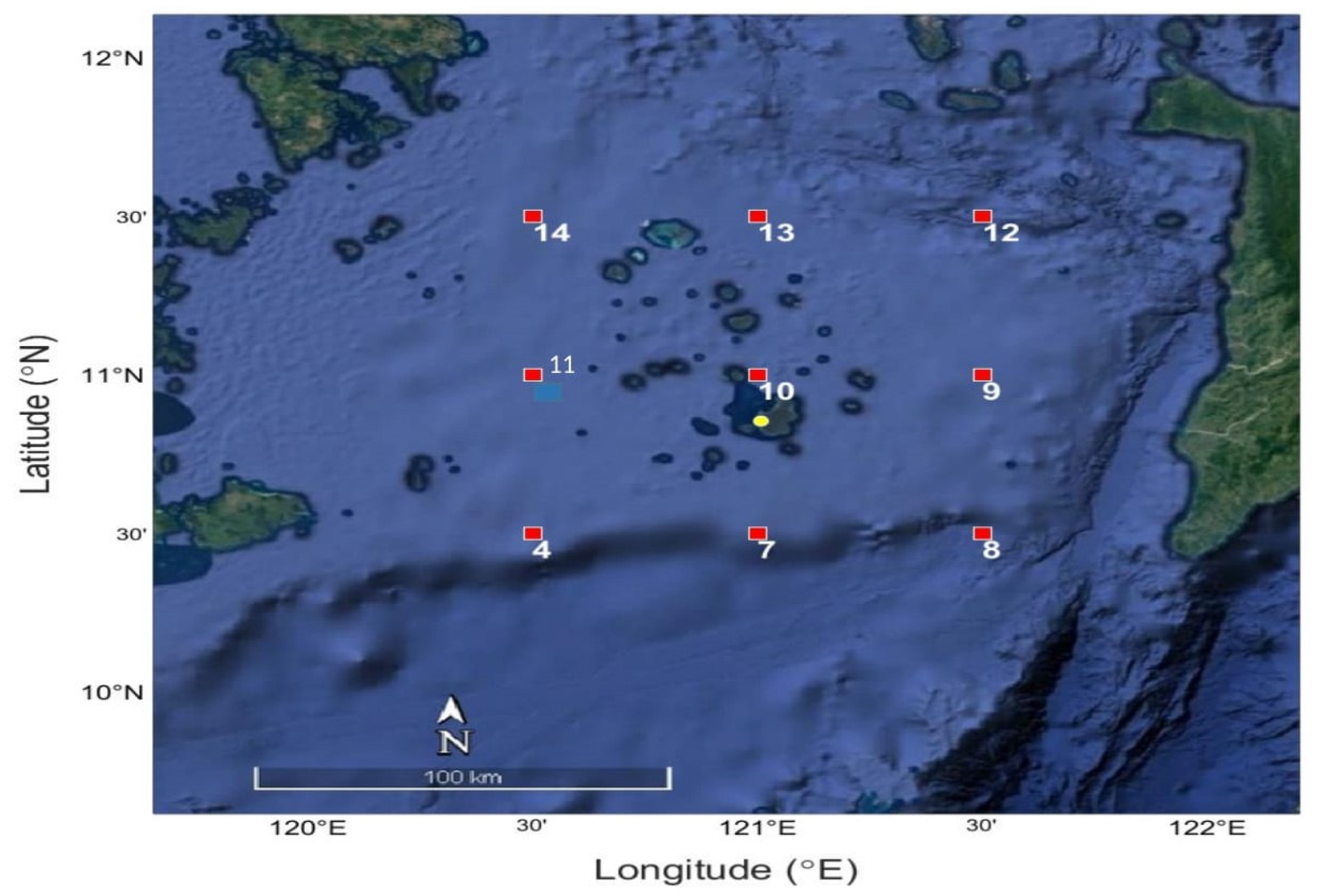
Figure 7.
Map of MOV stations (red squares) where 3-hourly data on wind velocity, Hs, Tp and Dp were extracted. On the other hand, the yellow circle is the PAGASA Cuyo station where daily wind data were recorded.
Figure 7.
Map of MOV stations (red squares) where 3-hourly data on wind velocity, Hs, Tp and Dp were extracted. On the other hand, the yellow circle is the PAGASA Cuyo station where daily wind data were recorded.
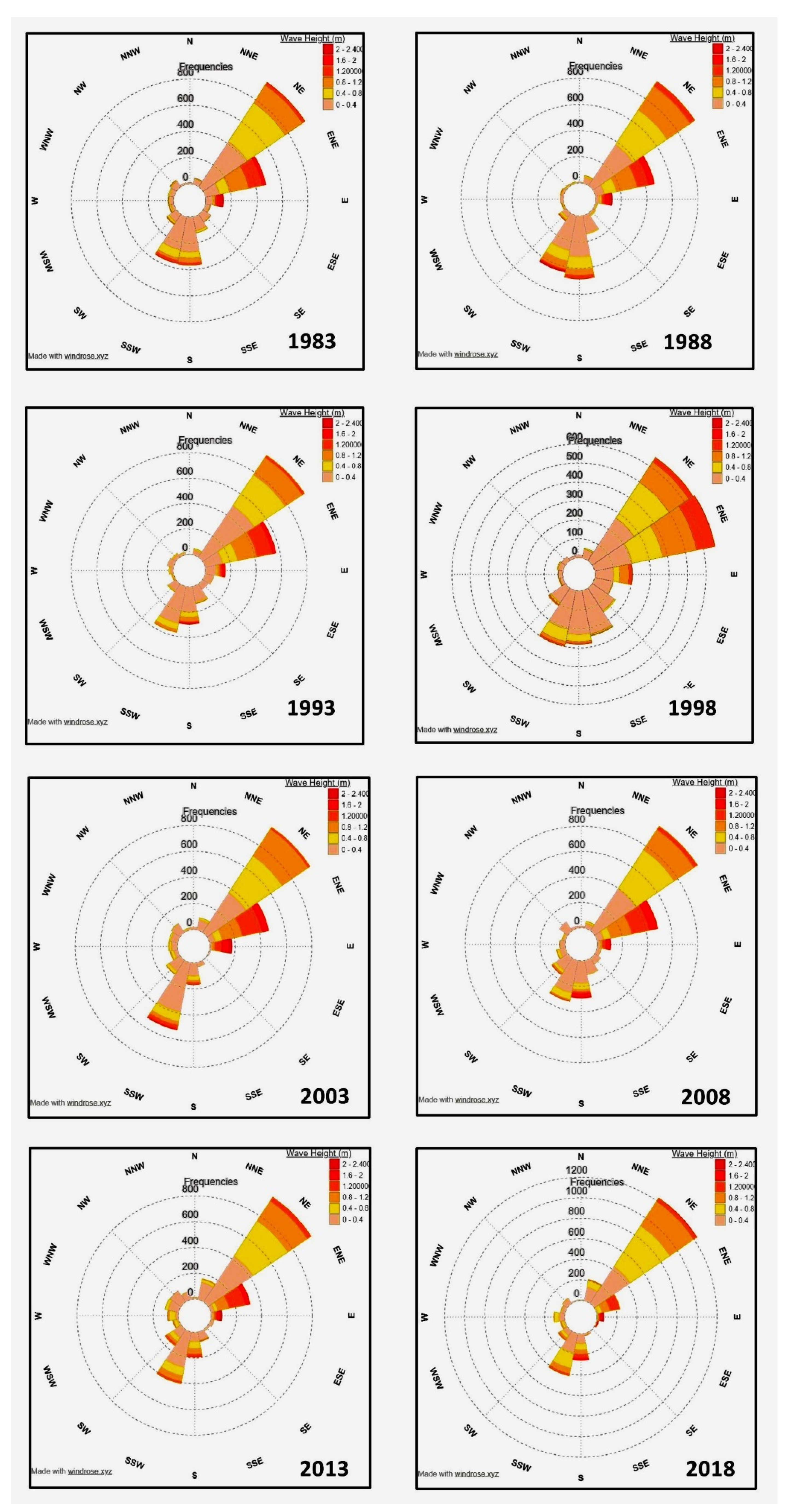
Figure 8.
Wave rose diagram at station 10 (11.0° N Lat., 121.0° E Long.) having a 5-year interval (data source: MOV).
Figure 8.
Wave rose diagram at station 10 (11.0° N Lat., 121.0° E Long.) having a 5-year interval (data source: MOV).
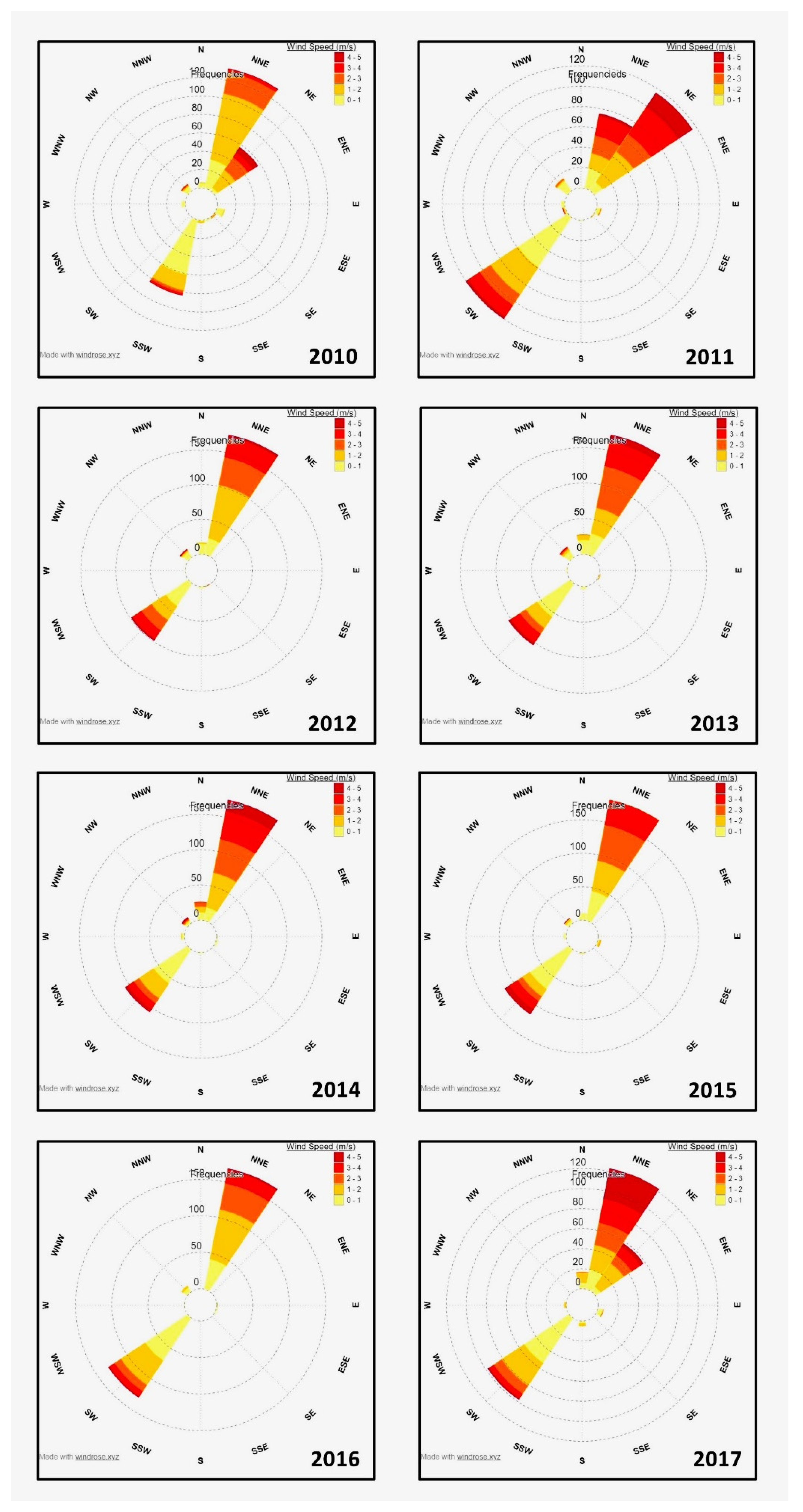
Figure 9.
Wind Rose diagram of PAGASA–Cuyo Station (10.85° N Lat., 121.04° E Long.) from 2010–2017 (data source: PAGASA–Cuyo Station).
Figure 9.
Wind Rose diagram of PAGASA–Cuyo Station (10.85° N Lat., 121.04° E Long.) from 2010–2017 (data source: PAGASA–Cuyo Station).
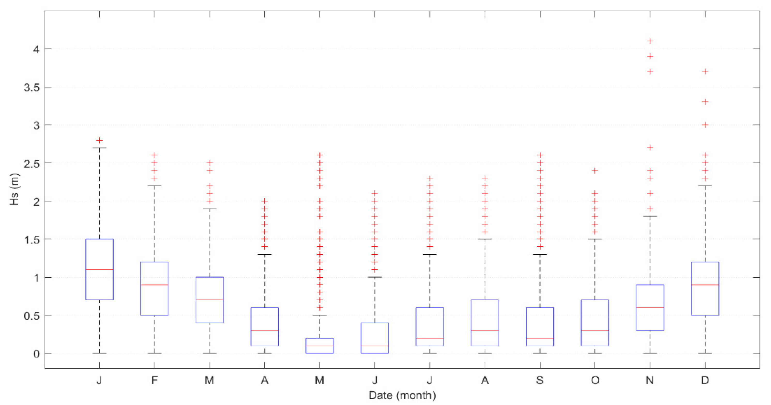
Figure 10.
Box-and-whisker plot (upper panel) and time-series plot (lower panel) of Hs from MOV. Red line inside the box of the box whisker plot shows the monthly median, box edges represent the 25th and 75th percentiles, the whiskers extend to the most extreme data points not considered outliers, while the red “+” marker symbol represents the outliers.
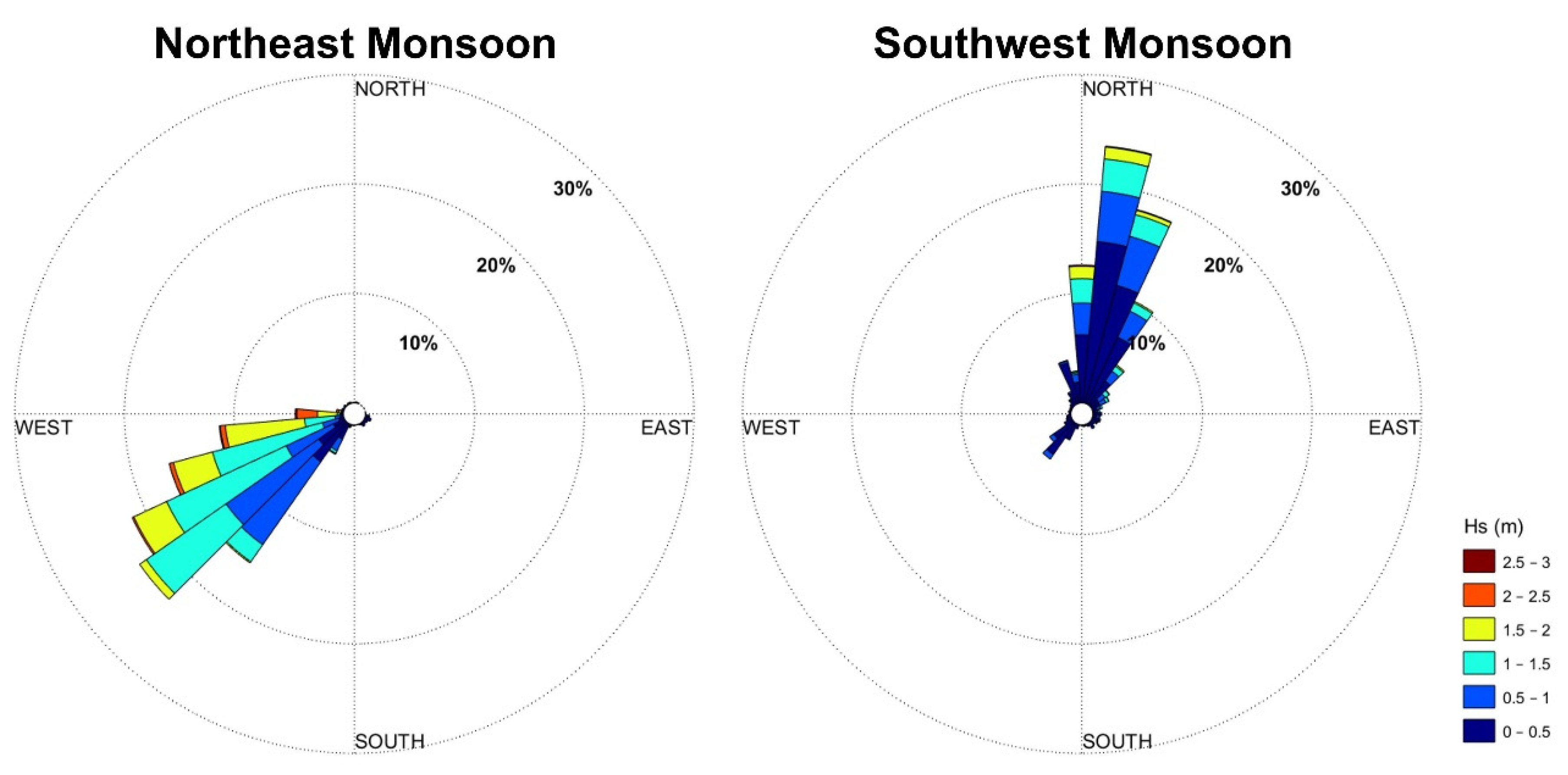
Figure 11.
Compass rose of Hs and Dp during the northeast and southwest monsoons.
Figure 11.
Compass rose of Hs and Dp during the northeast and southwest monsoons.
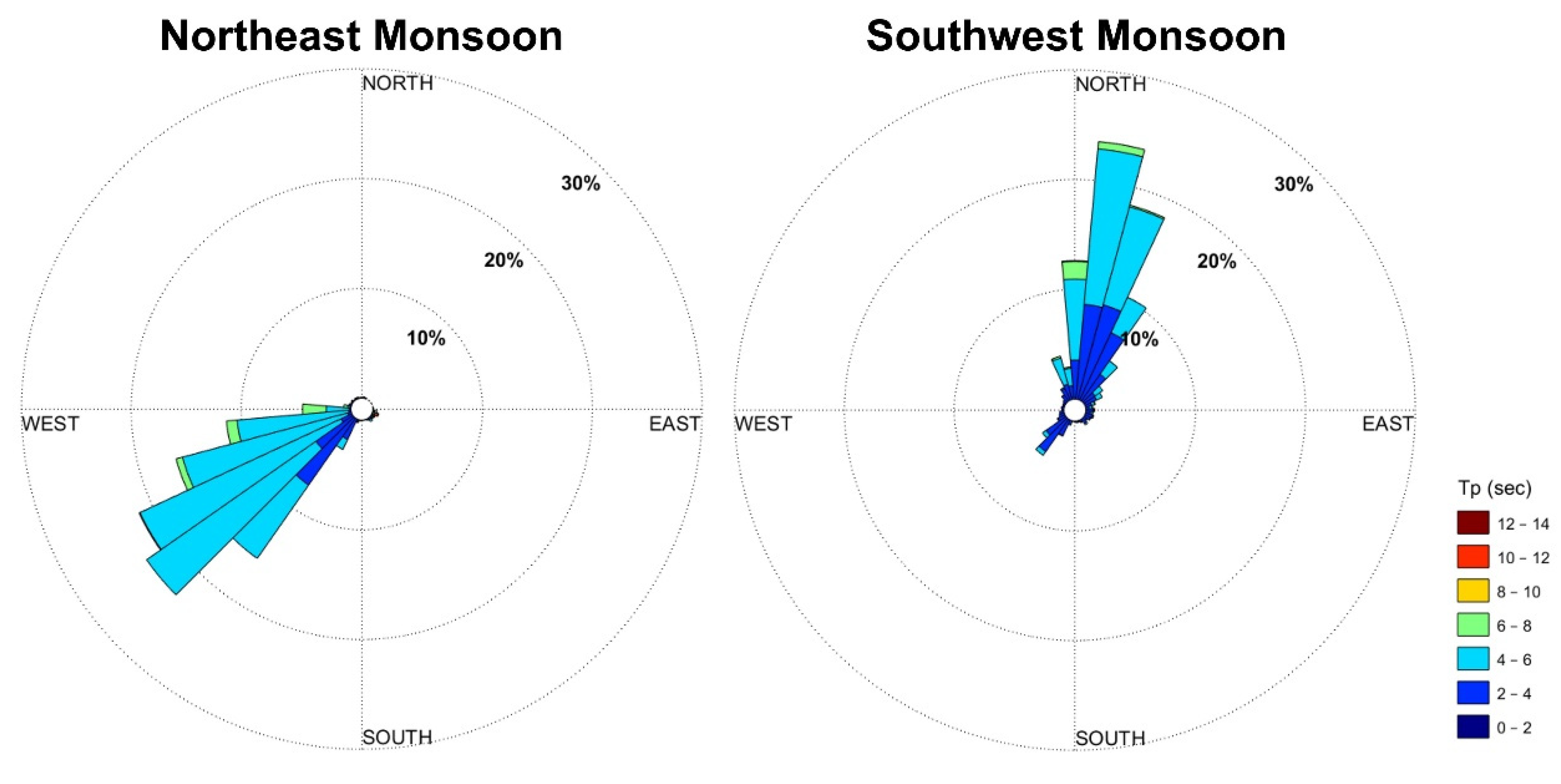
Figure 12.
Compass rose of Tp and Dp during the northeast and southwest monsoon.
Figure 12.
Compass rose of Tp and Dp during the northeast and southwest monsoon.
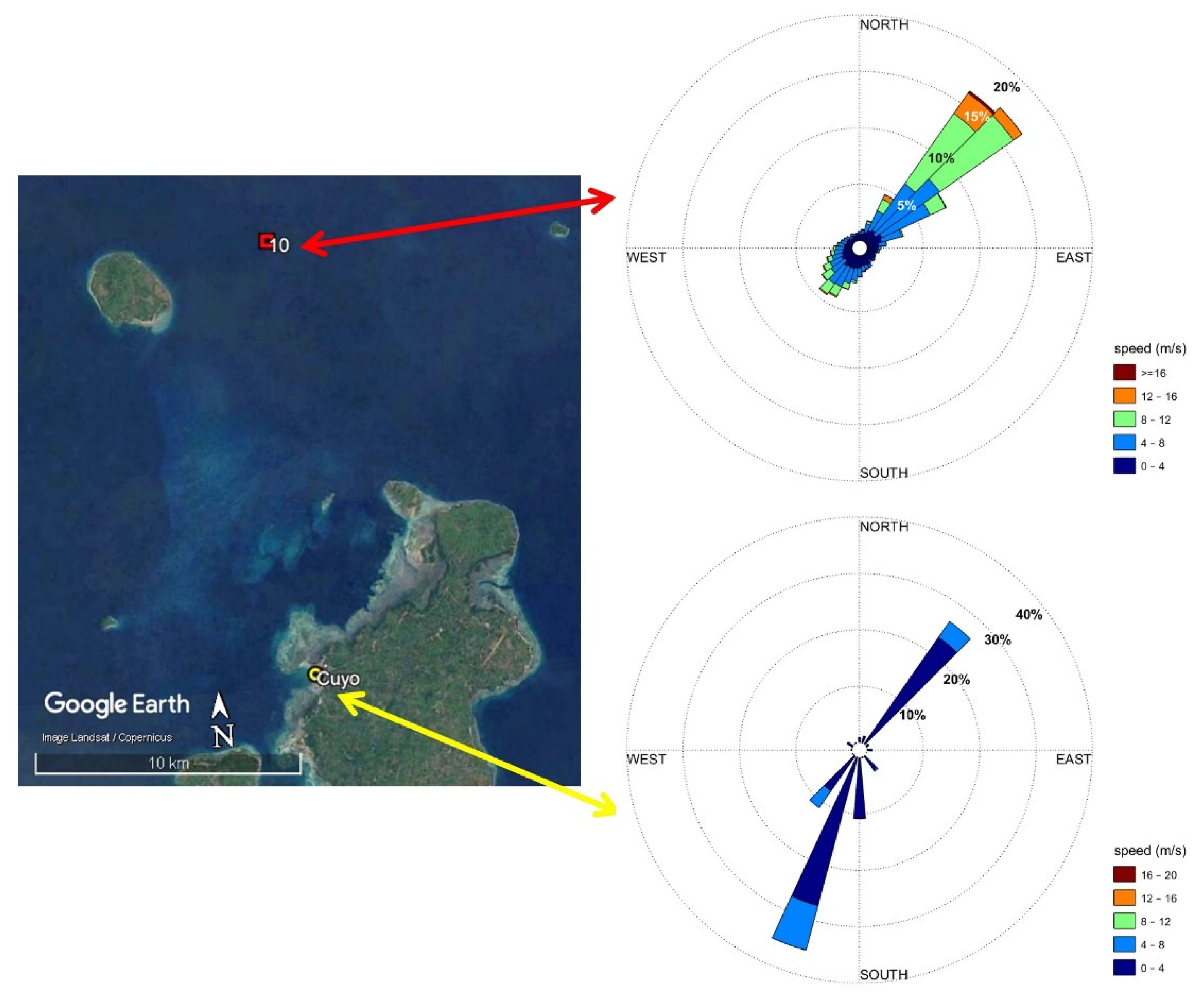
Figure 13.
Wind rose diagram of wind velocities using MOV data (upper right panel) and PAGASA data (lower right panel) with the location map of both stations.
Figure 13.
Wind rose diagram of wind velocities using MOV data (upper right panel) and PAGASA data (lower right panel) with the location map of both stations.
Figure 14.
Location of the six (6) points of interest within the model domain (stations A–F).
Figure 14.
Location of the six (6) points of interest within the model domain (stations A–F).
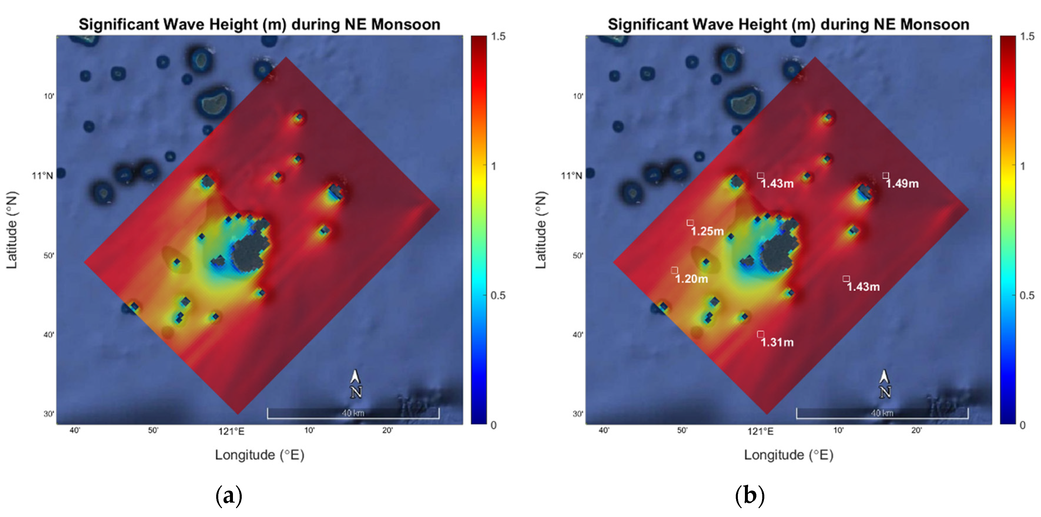
Figure 15.
(a) Hs (m) model during northeast monsoon season and (b) Hs model indicating the average Hs at stations A–F.
Figure 15.
(a) Hs (m) model during northeast monsoon season and (b) Hs model indicating the average Hs at stations A–F.
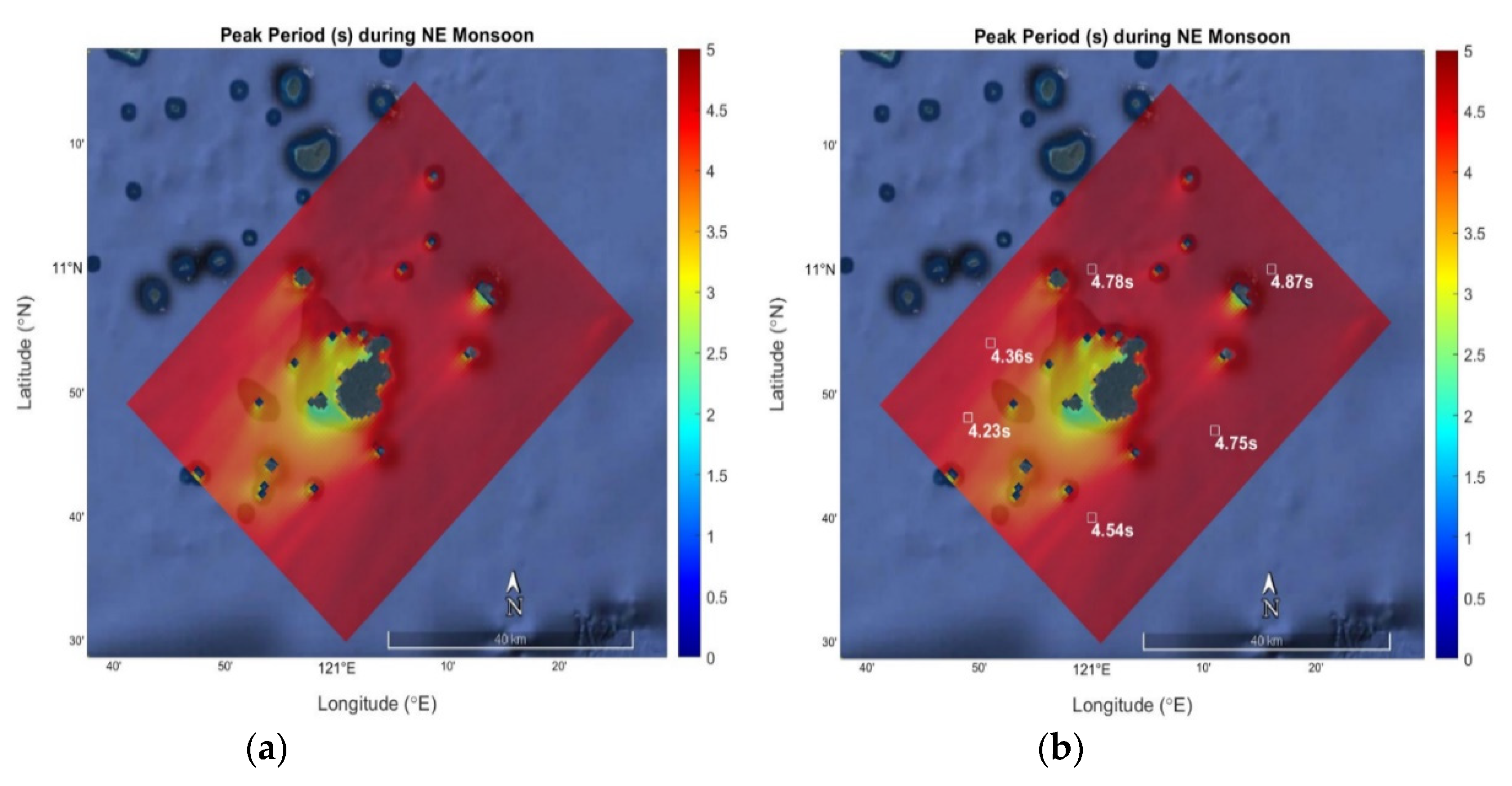
Figure 16.
(a) Tp (s) model during northeast monsoon season and (b) Tp model indicating the average Tp at stations A–F.
Figure 16.
(a) Tp (s) model during northeast monsoon season and (b) Tp model indicating the average Tp at stations A–F.
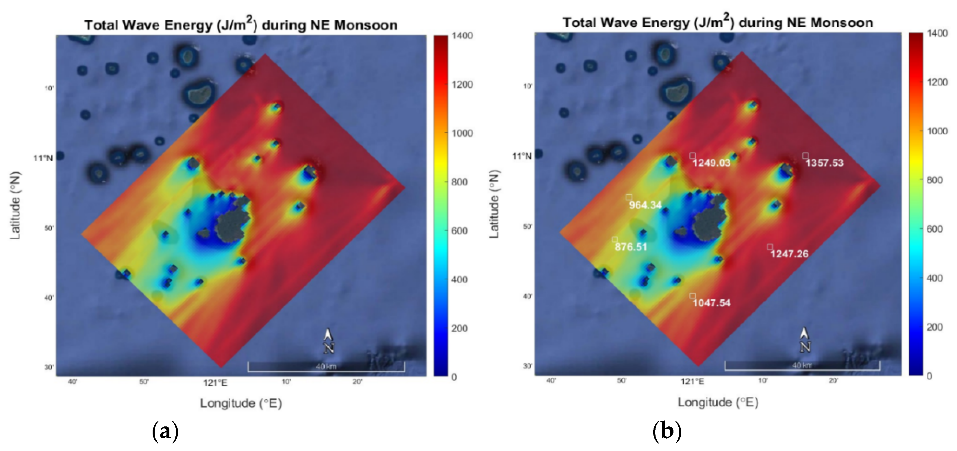
Figure 17.
(a) Wave energy propagation (J/m2) model during northeast monsoon season and (b) wave energy propagation model, indicating the total wave energy propagated and indicating the average period at stations A–F.
Figure 17.
(a) Wave energy propagation (J/m2) model during northeast monsoon season and (b) wave energy propagation model, indicating the total wave energy propagated and indicating the average period at stations A–F.
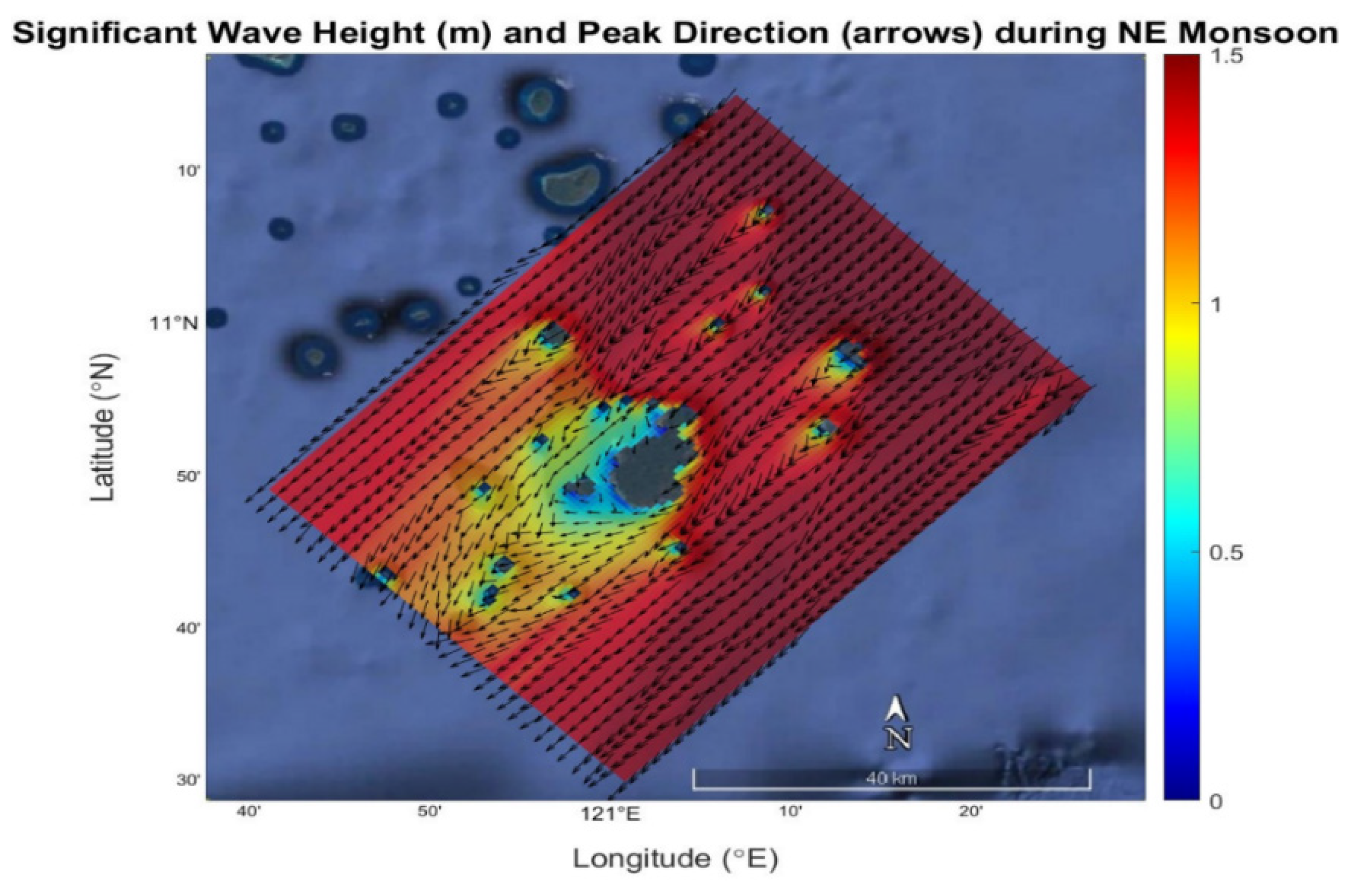
Figure 18.
Hs (m) and peak wind directions during northeast monsoon season.
Figure 18.
Hs (m) and peak wind directions during northeast monsoon season.
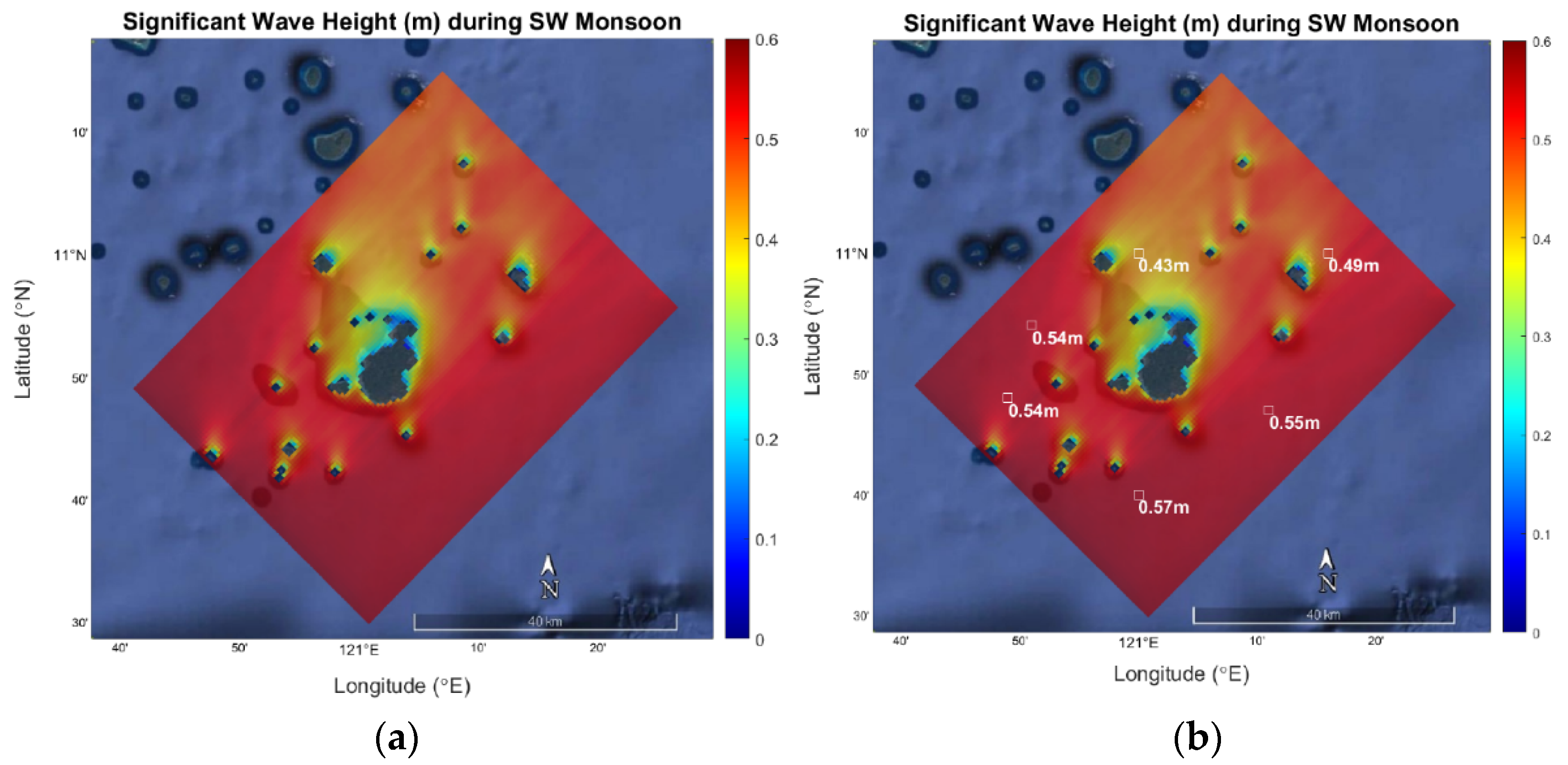
Figure 19.
(a) Hs (m) model during southwest monsoon season and (b) Hs model indicating the average Hs at stations A–F.
Figure 19.
(a) Hs (m) model during southwest monsoon season and (b) Hs model indicating the average Hs at stations A–F.
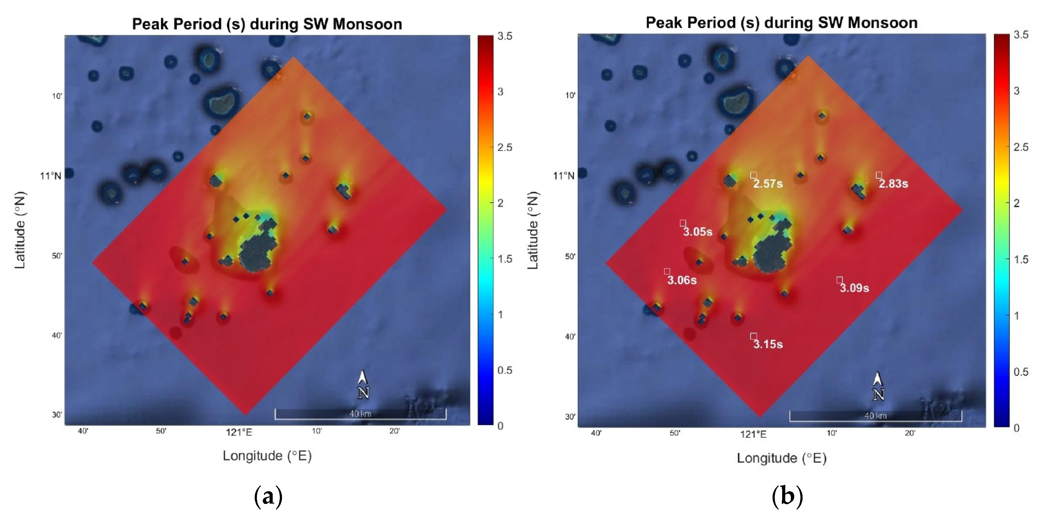
Figure 20.
(a) Tp (s) model during southwest monsoon season and (b) Tp model indicating the average Tp at stations A–F.
Figure 20.
(a) Tp (s) model during southwest monsoon season and (b) Tp model indicating the average Tp at stations A–F.
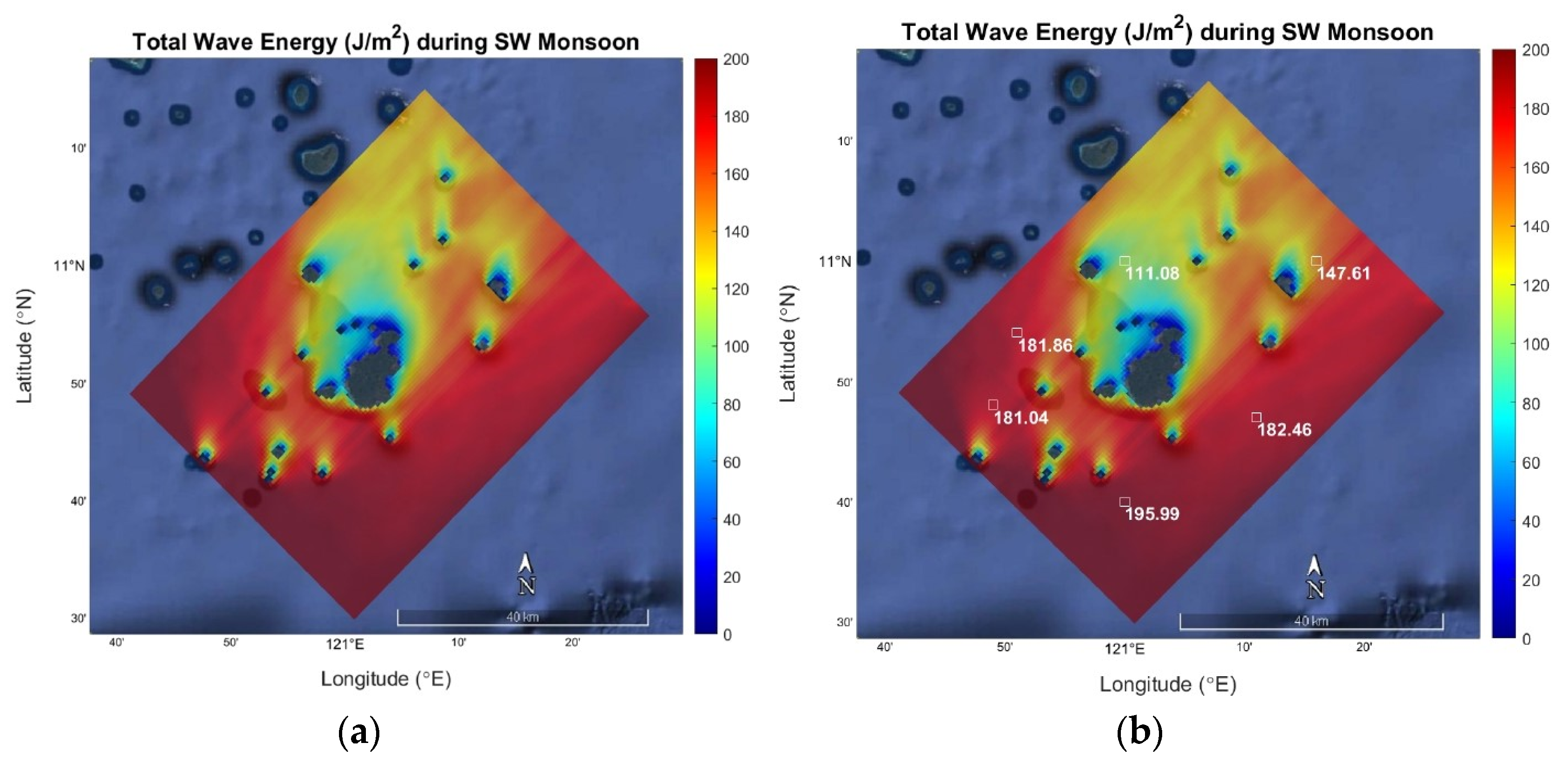
Figure 21.
(a) Wave energy (J/m2) model during southwest monsoon season and (b) wave energy model indicating the total wave energy at stations A–F during the season.
Figure 21.
(a) Wave energy (J/m2) model during southwest monsoon season and (b) wave energy model indicating the total wave energy at stations A–F during the season.
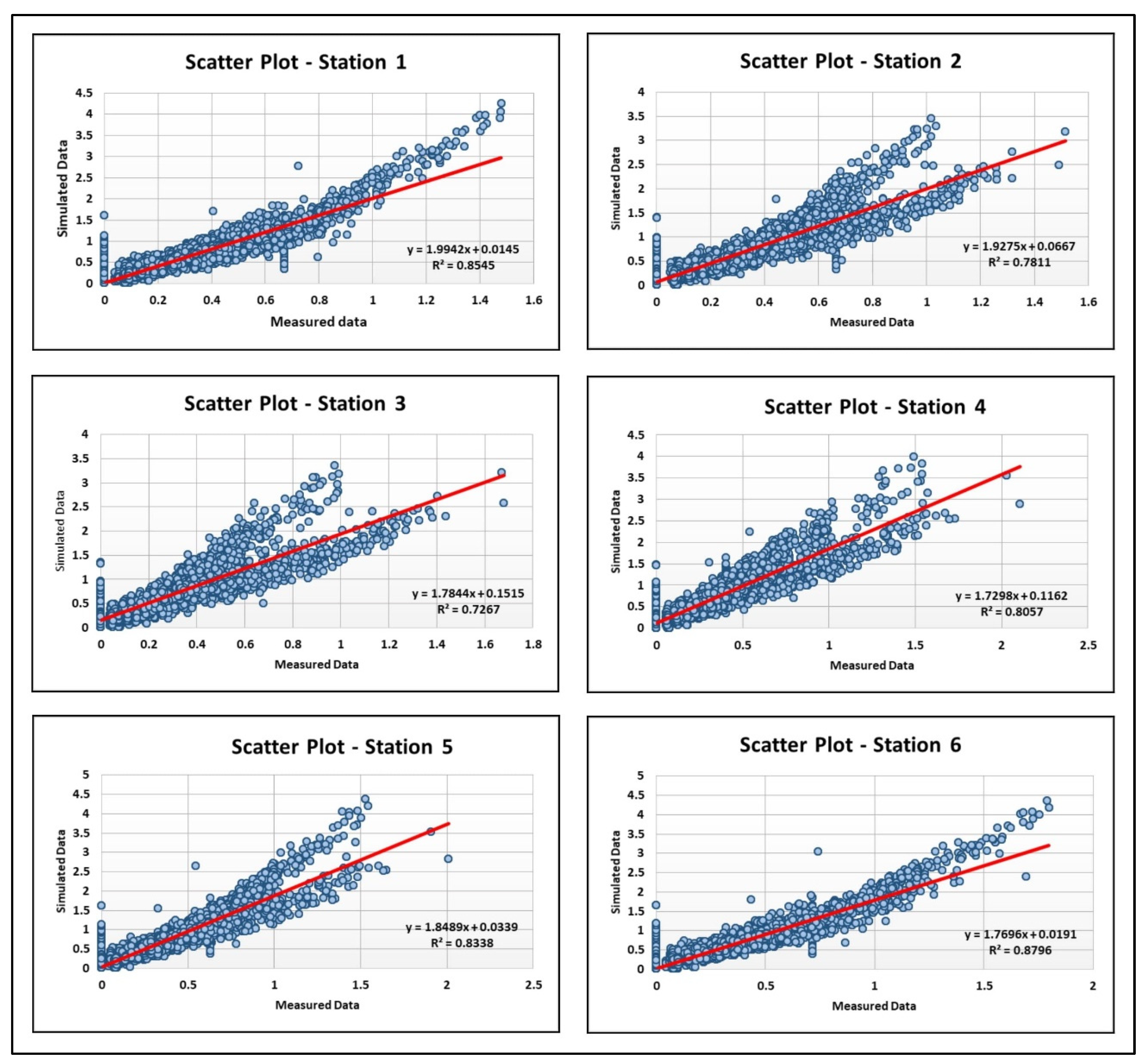
Figure 22.
Scatter plot graph of stations A–F graphically showing the correlation of the two parameters.
Figure 22.
Scatter plot graph of stations A–F graphically showing the correlation of the two parameters.
Table 1.
Mean Hs, Tp and Dp from MOV’s 2008–2018 data for the northeast (December–January–February (DJF)/Amihan) and southwest (June–July–August (JJA)/Habagat) monsoons.
Table 1.
Mean Hs, Tp and Dp from MOV’s 2008–2018 data for the northeast (December–January–February (DJF)/Amihan) and southwest (June–July–August (JJA)/Habagat) monsoons.
| Station | DJF Mean (Amihan) | JJA Mean (Habagat) |
|---|
| Hs | Tp | Dp | Hs | Tp | Dp |
|---|
| 4 | 1.1131 | 5.2592 | 46.6263 | 0.5066 | 4.1881 | −167.453 |
| 8 | 0.8601 | 4.8991 | 28.2988 | 0.5044 | 4.2172 | −150.142 |
| 12 | 1.106 | 4.8461 | 38.0907 | 0.4972 | 4.3267 | −153.027 |
| 14 | 1.1139 | 5.3135 | 62.773 | 0.4829 | 4.4801 | −164.637 |
Table 2.
Correlation between hindcast Hs data from MOV and PAGASA measured wind speed.
Table 2.
Correlation between hindcast Hs data from MOV and PAGASA measured wind speed.
| Station | Distance from PAGASA—Cuyo Station (km) | Correlation Factor (r) | Average Annual Hs (m) | Average Annual Pd (kW/m) |
|---|
| 4 | 68 | 0.71 | 1.34 | 4.28 |
| 7 | 40 | 0.6 | 1.11 | 2.66 |
| 8 | 66 | 0.51 | 1.17 | 3.06 |
| 9 | 56 | 0.66 | 1.16 | 3.05 |
| 10 | 15 | 0.75 | 1.20 | 3.13 |
| 11 | 60 | 0.76 | 1.44 | 5.00 |
| 12 | 92 | 0.75 | 1.38 | 4.25 |
| 13 | 72 | 0.73 | 1.44 | 4.88 |
| 14 | 92 | 0.62 | 1.40 | 4.88 |
Table 3.
Studies conducted that validate MOV’s data.
Table 3.
Studies conducted that validate MOV’s data.
| MOV’s Wave Hindcast Validation | Results | Year | Source |
|---|
| Hindcast significant wave height was validated against (1) altimeters in the entire Tanaki grid area and (2) wave rider buoy moored ~17 m deep near the port of Tanaki. | 1. Model Hs does not reveal significant or systematic errors and shows satisfactory overall performance of the wave model. | 2021 | [45] |
| 2. Results of the model data validation against the buoy were also in good agreement, especially when considering the proximity of the buoy to shore and the mooring’s relatively shallow depth (Hs, r = 0.933, Tp, r = 0.624). |
| The mean monthly distribution of significant wave height from MOV was validated against the wave data from FugroGeos for the Central–Southern North Sea region. | 1. The coefficient of correlation is satisfactory at r = 0.55. | 2021 | [46] |
| Assessment of the suitability of the hindcast directional wave spectra data in the northern and southern hemisphere was compared against buoy observations from National Oceanic and Atmospheric Observation’s National Data Buoy Center. | 1. The Hs time series obtained from the hindcast and the observations are well correlated (rHs > 0.8 for all the selected buoys). | 2019 | [47] |
| 2. The RMSE values are within 10% of the maximum value attained by the model for all the selected buoys |
| 3. The monthly mean spectra from model and observations are well correlated, with r ~0.9. |
| A report on meteorological and oceanographic conditions at Astrolabe Reef prepared by MetOcean Solutions Limited has been reviewed by NIWA. These statistics are derived from numerical model simulations, which were first validated against available data for winds, waves and currents | 1. The verification of significant wave heights against measurements is satisfactory. It gives some confidence in the accuracy of the hindcast winds, in the absence of direct verification at a nearby location in the Bay of Plenty. | 2013 | [48] |
Table 4.
Summary results of wave parameters for the NE and SW monsoons at the six (6) points of interest near the island (simulated using MOV data).
Table 4.
Summary results of wave parameters for the NE and SW monsoons at the six (6) points of interest near the island (simulated using MOV data).
| Sta | Lon | Lat | DJF-NE Monsoon | JJA-SW Monsoon |
|---|
| Hs (m) | Tp (s) | Total Wave Energy (J/m2) | Pd (W/m) | Hs (m) | Tp (s) | Total Wave Energy (J/m2) | Pd (W/m) |
|---|
| A | 121 | 11 | 1.428 | 4.7781 | 1249.04 | 3978.25 | 0.4258 | 2.5658 | 111.0763 | 193.8773 |
| B | 120.85 | 10.9 | 1.2547 | 4.361 | 964.3382 | 2789.88 | 0.5449 | 3.0525 | 181.8621 | 379.0649 |
| C | 121 | 10.67 | 1.1962 | 4.2348 | 876.5134 | 2361.11 | 0.5437 | 3.0582 | 181.0445 | 366.3609 |
| D | 121.18 | 10.78 | 1.3077 | 4.5399 | 1047.54 | 3250.23 | 0.5657 | 3.1477 | 195.9928 | 420.4111 |
| E | 121.27 | 11 | 1.427 | 4.746 | 1247.26 | 3910.13 | 0.5458 | 3.0908 | 182.4629 | 388.3967 |
| F | 120.82 | 10.8 | 1.4887 | 4.871 | 1357.53 | 4246.80 | 0.4909 | 2.834 | 147.609 | 280.2246 |
Table 5.
Summary results of wave parameters for the NE and SW monsoons at the nine (9) MOV stations.
Table 5.
Summary results of wave parameters for the NE and SW monsoons at the nine (9) MOV stations.
| Sta | Lon | Lat | DJF-NE Monsoon | JJA-SW Monsoon |
|---|
| Hs (m) | Tp (s) | Total Wave Energy (J/m2) | Pd (W/m) | Hs (m) | Tp (s) | Total Wave Energy (J/m2) | Pd (W/m) |
|---|
| 14 | 120.5 | 11.5 | 1.4042 | 4.7092 | 1207.84 | 3968.37 | 0.5654 | 3.0135 | 195.8246 | 419.0981 |
| 13 | 121 | 11.5 | 1.4408 | 4.6642 | 1271.41 | 3891.82 | 0.5154 | 2.7885 | 162.6904 | 299.367 |
| 12 | 121.5 | 11.5 | 1.3 | 4.3625 | 1035.14 | 2968.29 | 0.5552 | 2.9305 | 188.8014 | 366.2484 |
| 11 | 120.5 | 11 | 1.4885 | 4.7751 | 1357.16 | 4280.96 | 0.5849 | 3.0785 | 209.5412 | 431.2502 |
| 10 | 121 | 11 | 1.5135 | 4.8353 | 1403.07 | 4513.25 | 0.5274 | 2.8493 | 170.3466 | 331.3767 |
| 9 | 121.5 | 11 | 1.4505 | 4.6481 | 1288.67 | 3923.06 | 0.5835 | 3.0309 | 208.5396 | 420.899 |
| 4 | 120.5 | 10.5 | 1.5487 | 4.8773 | 1469.17 | 4690.35 | 0.6025 | 3.1567 | 222.3052 | 484.0884 |
| 7 | 121 | 10.5 | 1.5058 | 4.8147 | 1388.73 | 4501.62 | 0.5889 | 3.0644 | 212.4356 | 436.9373 |
| 8 | 121.5 | 10.5 | 1.4317 | 4.6555 | 1255.57 | 3879.12 | 0.5759 | 3.0252 | 203.1603 | 411.3036 |
Table 6.
Summary of statistical metrics between “observed values” and “hindcast parameters”.
Table 6.
Summary of statistical metrics between “observed values” and “hindcast parameters”.
| Station | | | Bias | RMSE | SI | r |
|---|
| A | 0.40 | 0.80 | 0.40 | 0.55 | 1.38 | 0.92 |
| B | 0.37 | 0.79 | 0.41 | 0.54 | 1.45 | 0.88 |
| C | 0.35 | 0.77 | 0.37 | 0.54 | 1.58 | 0.85 |
| D | 0.41 | 0.82 | 0.41 | 0.54 | 1.32 | 0.90 |
| E | 0.45 | 0.86 | 0.42 | 0.56 | 1.24 | 0.91 |
| F | 0.47 | 0.86 | 0.38 | 0.51 | 1.08 | 0.94 |
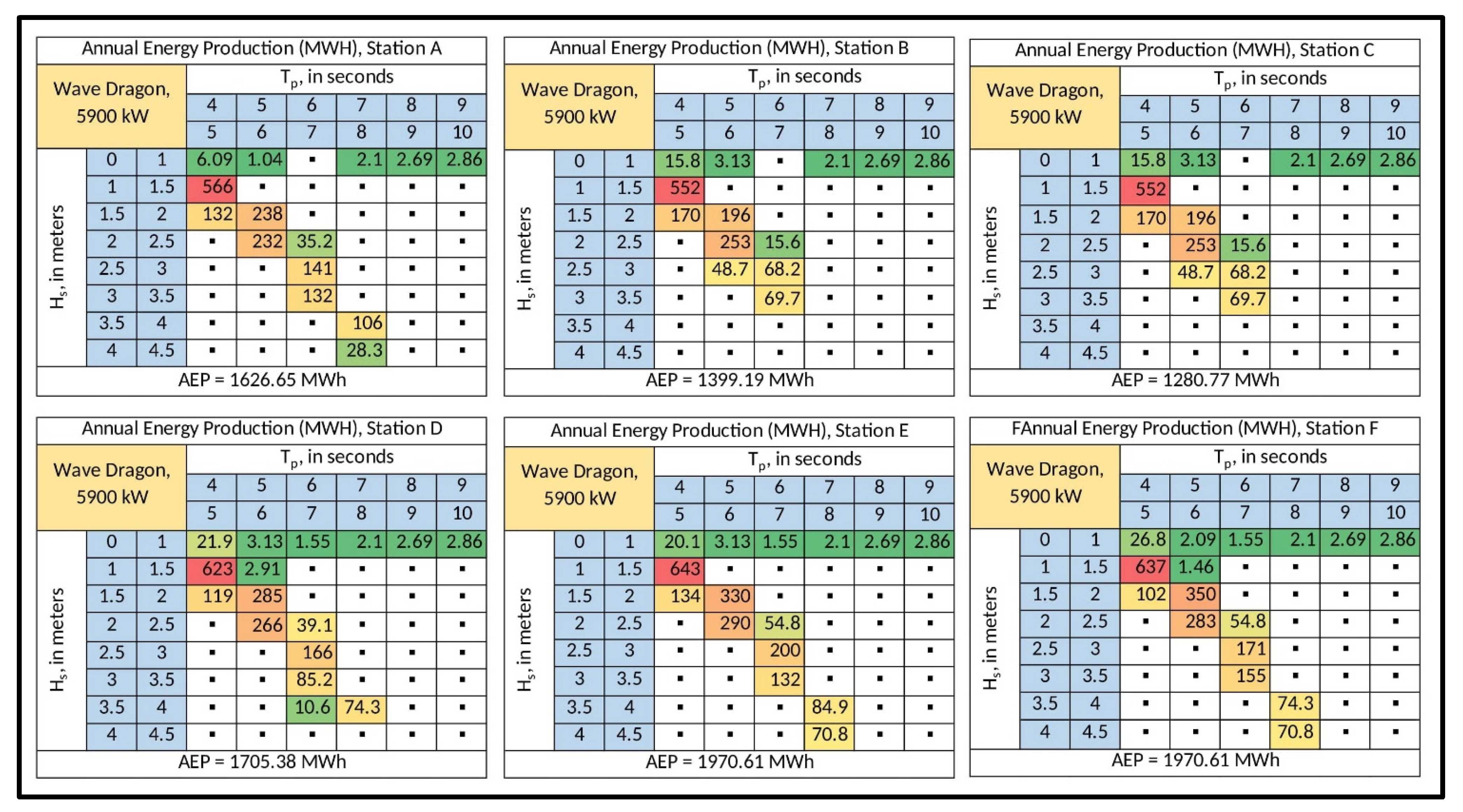
Table 7.
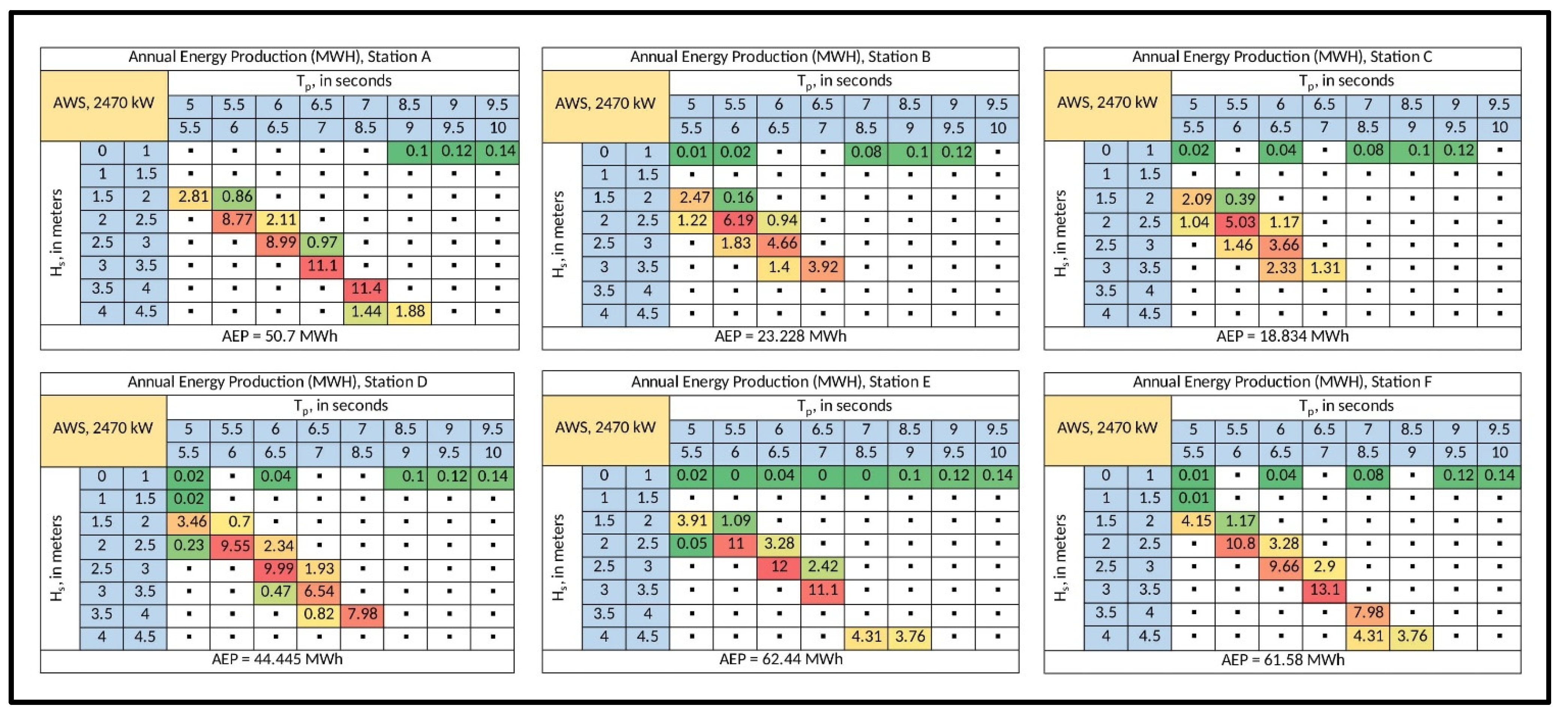
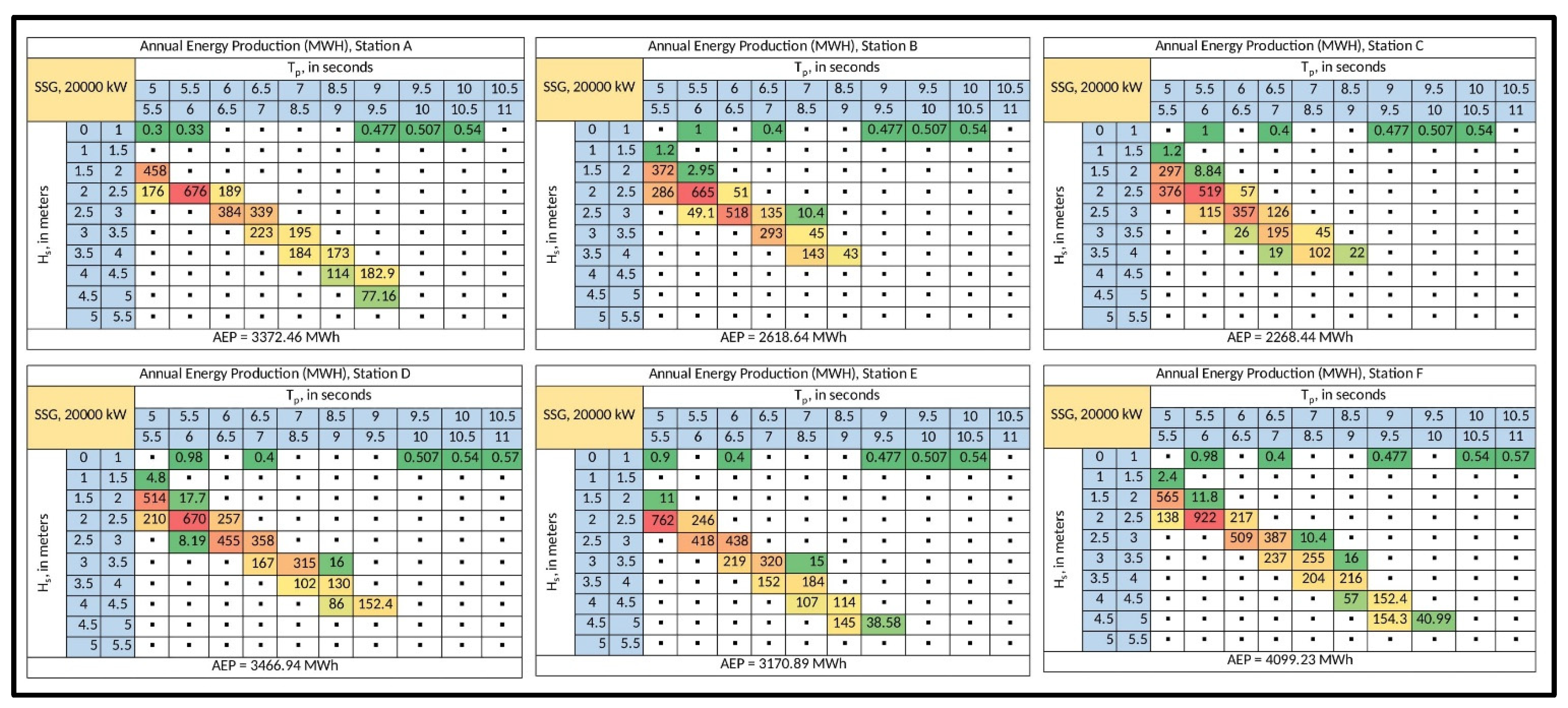
AEP results of Wave Dragon, AWS and SSG, in MWh.
Table 7.
AEP results of Wave Dragon, AWS and SSG, in MWh.
| Wave Energy Converter | Annual Energy Production (AEP), in MWh | Capacity Factor (%) |
|---|
| A | B | C | D | E | F |
|---|
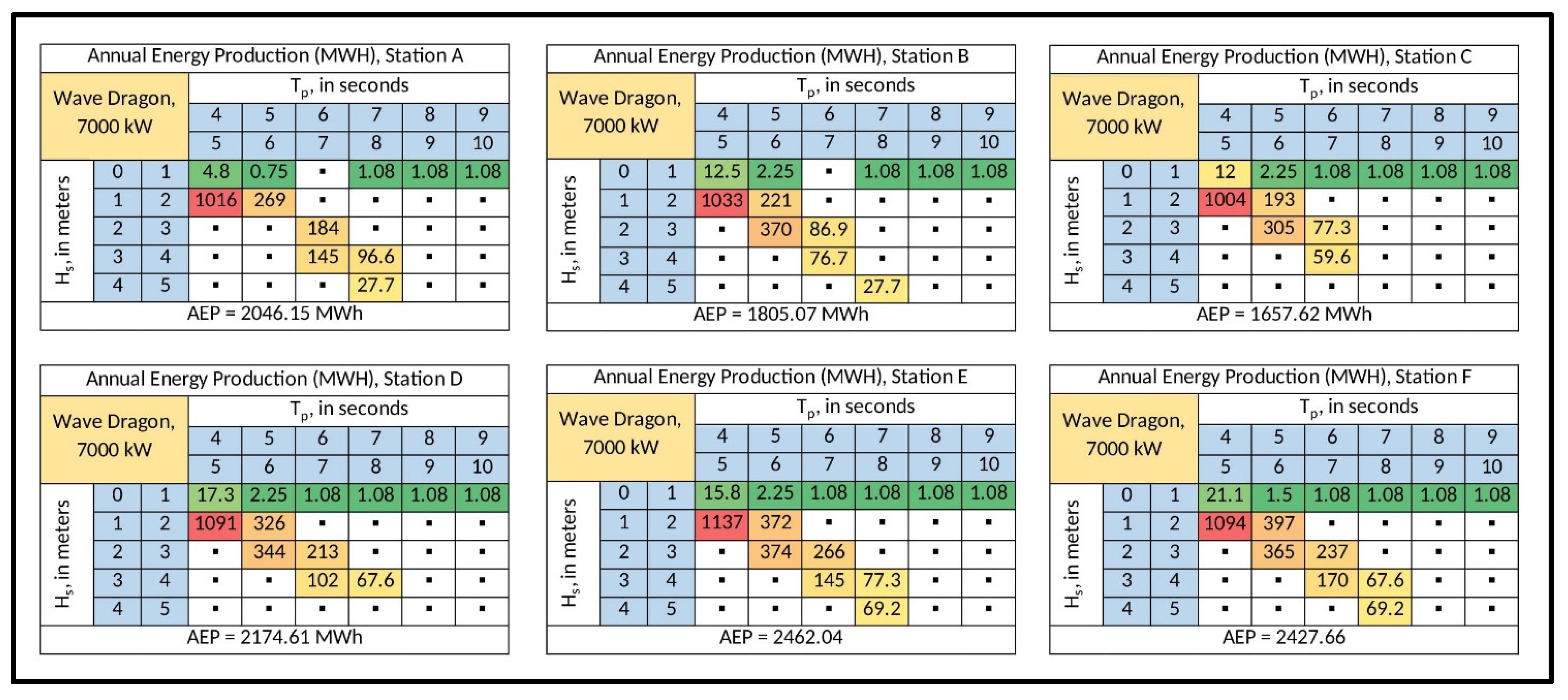
| Wave Dragon, 5900 kW | 1626.65 | 1399.19 | 1280.77 | 1705.38 | 1970.61 | 1937.01 | 3.1 |
| Wave Dragon, 7000 kW | 2046.15 | 1805.07 | 1657.62 | 2174.61 | 2462.04 | 2427.66 | 3.4 |
| Archimedes Wave Swing, 2470 kW | 50.754 | 23.118 | 18.834 | 44.445 | 62.424 | 61.584 | 0.2 |
| Seawave Slot-Cone Generator, 20,000 kW | 3322.45 | 2618.643 | 2268.44 | 3466.91 | 3170.892 | 4099.23 | 1.8 |
Table 8.
Sample computation of AEP for Wave Dragon (7000 kW) at Station F.
Table 8.
Sample computation of AEP for Wave Dragon (7000 kW) at Station F.
| Annual Energy Production |
|---|
| Wave Dragon, 7000 kW | Tp, in seconds |
| 4 | 5 | 6 | 7 | 8 | 9 |
| 5 | 6 | 7 | 8 | 9 | 10 |
Hs,
in meters | 0 | 1 | 21.12 | 1.5 | 1.08 | 1.08 | 1.08 | 1.08 |
| 1 | 2 | 1094 | 396.9 | | | | |
| 2 | 3 | | 365.4 | 236.7 | | | |
| 3 | 4 | | | 170.4 | 67.62 | | |
| 4 | 5 | | | | 69.15 | | |
| AEP = 2427.48 MWh |


 ,
, 


