Article

Full-Scale Digesters: Model Predictive Control with Online Kinetic Parameter Identification Strategy

1
Departamento de Tecnología Electrónica, Escuela Politécnica, Universidad de Sevilla, 41011 Seville, Spain
2
Efuels Technologies Ltd., 42-44 Bishopgate, London EC2N 4AH, UK
3
Departamento de Ingeniería Química, Campus de Cantoblanco, Universidad Autonoma de Madrid, 28049 Madrid, Spain
4
Facultad de Minas, Universidad Nacional de Colombia, Robledo, Medellín 050034, Colombia
*
Author to whom correspondence should be addressed.
Energies 2022, 15(22), 8594; https://doi.org/10.3390/en15228594
Submission received: 21 August 2022 / Revised: 9 November 2022 / Accepted: 10 November 2022 / Published: 16 November 2022

Abstract

:
This work presents a nonlinear model predictive control scheme with a novel structure of observers aiming to create a methodology that allows feasible implementations in industrial anaerobic reactors. In this way, a new step-by-step procedure scheme has been proposed and tested by solving two specific drawbacks reported in the literature responsible for the inefficiencies of those systems in real environments. Firstly, the implementation of control structures based on modeling depends on microorganisms’ concentration measurements; the technology that achieves this is not cost-effective nor viable. Secondly, the reaction rates cannot be considered static because, in the extended anaerobic digestion model (EAM2), the large fluctuation of parameters is unavoidable. To face these two drawbacks, the concentration of acidogens and methanogens, and the values of the two reaction rates considered have been estimated by a structure of two observers using data collected by sensors. After 90 days of operation, the error in convergence was lower than 5% for both observers. Four model predictive controller (MPC) configurations are used to test all the previous information trying to maximize the volume of methane and demonstrate a satisfactory operation in a wide range of scenarios. The results demonstrate an increase in efficiency, ranging from 17.4% to 24.4%, using as a reference an open loop configuration. Finally, the operational robustness of the MPC is compared with simulations performed by traditional alternatives used in industry, the proportional-integral-derivative (PID) controllers, where some simple operational scenarios to manage for an MPC are longer sufficient to disrupt a normal operation in a PID controller. For this controller, the simulation shows an error close to the 100% of the reference value.

1. Introduction

The main attribute of industrial processes and manufacturing is the large-scale transformation of mass and energy into high-end valuable specific materials and compounds [1]. In essence, chemical and biological processes are imperative for those purposes because it is primarily at this stage where the elements in a reaction can be manipulated to achieve the desired attributes [2,3,4]. All the above is possible if a control and monitoring scheme is added to guarantee safe and stable operation [5]. Specifically, in anaerobic systems, the transformation of substrates into biogas and digestate has attractive advantages in comparison to classical alternatives such as aerobic digestion or composting [6,7]; it returns little sludges, has a positive overall energy balance, and also has enormous potential to reduce challenging and concentrated substrates such as animal wastes [8,9]. However, this is an elaborated biochemical process that includes diverse microorganisms, making the process nonlinear [10]. In this area, it is great of interest to derive models that would be as sensitive as possible to the lack of phenomenological knowledge [11,12]. Thus, an interesting alternative to represent this phenomenon is the extended anaerobic digestion mathematical model 2 (EAM2) [13], designed for control and monitoring purposes. It circumvents the difficulties in locating the biological lack of knowledge in dedicated terms, namely reaction rates [14]. Additionally, compared with its predecessor, in the anaerobic digestion mathematical model 2 (AM2), two additionally yield parameters were included to consider the influence of proteins and aminoacids on the dynamic of alkalinity and consider more substrates to be modeled.
In order to allocate a strategy that better fits the challenge mentioned above, several techniques have been proposed from different control areas. Some of them are nonlinear proportional-integral-derivative (PID) controllers, linear quadratic regulation (LQR) for nonlinear systems [15], nonlinear model predictive control (NMPC) [16], and receding horizon controllers [17,18], to name the most relevant cases reported in the literature. Although these strategies have proven to be effective, the remaining inefficiencies surge from the fact that some of the parameters are not available to be measured online, and the concentrations of the microorganisms cannot be measured periodically because on-site analytical procedures are challenging to perform [5]. A nonlinear model-based control scheme has been proposed to achieve a satisfactory operation. At the same time, the representation of anaerobic digestion (AD) processes is reduced to a minimal number of assumptions in the model-building exercise, maintaining the performance [18,19]. Among the alternatives registered in the literature, the Model Predictive Control (MPC) [17,18] offers several benefits compared with traditional methods [14,20,21]. This algorithm uses a mathematical model to predict and follow the system’s evolution in advance. One of the main advantages is the explicit use of physical and operational constraints in the controller, allowing it to stand around working under feasible operational conditions [22,23].
To achieve this objective, a necessary condition must be satisfied to unlock the door and enable the operation of control schemes based on modeling. All the information needed from the anaerobic reactor must be available periodically, so a group of reliable sensors should be considered to measure, in real-time, the evolution of reactions in the homogeneous reaction system [24]. Some key variables, the concentrations of microorganisms, as well as the growth rates of reactions (considered variable due to the large fluctuation of parameters in AM2 [10]), are usually tested using analytical methods through specialized laboratories on-site. The cost and duration of these analyses limit the frequency of the sampling [25]. Additionally, the available online sensors on the market for biomass or metabolites need to be adequate for regular industrial applications [14]. The previous assumption sets a significant challenge because collecting this information is critical for the operation of the controller algorithm. In general, the unavailability of specialized instruments incentive the design and construction of observers dedicated to the reaction process. Hence, the design of software sensors, based on the available measurements [14,26], allows to guarantee a streamline of information between the reactor and the control algorithm [27].
State and parameter observers established over accurate and strict models are the best alternatives to find a way to obtain the lack of the data needed [28,29,30]. For anaerobic reaction processes, the nonlinear AM2 has been widely proven for monitoring and control purposes [10,13]. This model, constructed under a mass-balance framework, can adapt its dynamics to various AD configurations of reactors and elude the drawback related to the absence of phenomenological knowledge, concentrating this information in non-sensitiveness-dedicated terms named reaction rates [10,23]. The complexity of the biochemical process considers different types of microorganisms, making the process nonlinear and unpredictable, impractical for the traditional online estimation strategies, especially if the operation of the homogeneous system is conditioned by constraints [5]. To deal with these inconveniences, a sequential structure in cascade has been proposed [14]. The main idea is to estimate the concentration of acidogens and methanogens in the absence of reaction rates. Then, the next step is to use this information to perform a new observation that estimates the reaction rates. Acquiring in-depth knowledge of the evolution of reaction rates represents a challenge since it reveals the degree of completion of both reactions during the process [5,31].
This paper is organized as follows. Section 2 explains the extended AM2 mathematical model used for control purposes, where additional terms are included due to the influence of proteins and aminoacids on the dynamics of alkalinity. The modification of the AM2 model [10] unlocks the door to add a broad spectrum of substrates allowed to be used by the control algorithm. Then, Section 3 presents the parameter identification procedure based on optimization that uses a novel step-ahead algorithm to considerably improve the efficiency of adjusting the dynamics of the model to the data. The asymptotic state observer that operates without information on the reaction rates is presented to estimate the concentrations of acidogens and methanogens. Next, using the previous information, a second observer estimates the evolution of the two reaction rates considered. In Section 4, the information taken from observers and the reactor’s measurements is used to enable the operation of the MPC. Finally, Section 5 shows the improvement achieved by using the MPC controller, measuring the increase in the volume of methane produced. The robustness of the MPC proposed is compared with the PID controller.

2. Optimal Parameter Identification Algorithm

The model EAM2, initially proposed by Bernard et al. [10] as AM2 in 2002 and modified by Cortés et al. [13] in 2022, was selected to support the new monitoring and control structure presented in this paper. The new model solves two issues documented in the literature as the main drawbacks in implementing automated decision support systems on anaerobic reactors [11]. First, the necessity to characterize the inlet substrate [10]. EAM2 considers a wider range of substrates than AM2 because it takes into account the effect of ammonium produced from proteins and aminoacids that affect the dynamics of alkalinity. Second, the concentrations of acidogens and methanogens are estimated using a specific state observer. The above-mentioned solutions allow balancing the absence of reliable sensors or analytical methods to obtain the needed information periodically [10].

2.1. Proposed Mass-Balance Mathematical Model for Anaerobic Reactors

The extended mathematical model used in this paper is based on the AD represented by two main groups of microorganisms. Two consecutive process describe the AD phenomenon on reactors, the acidogenic bacteria (represented by X 1 ) that consume the organic substrate (represented by S 1 ) and produce mainly volatile fatty acids (mainly acid acetic, represented by S 2 ). Thus, the second group of microorganisms, the methanogenic archaea (represented by X 2 ), consumes S 2 and produces CO 2 and CH 4 .
Two yield parameters were added to represent the generation of ammonium due to the fermentation of aminoacids or the consumption by the growth of microorganisms. The terms added are K Z , 1 and K Z , 2 , respectively. The model presented in Cortés et al. [13] considers the following dynamical equations:
d X 1 d t = X 1 ( μ 1 α D )
d X 2 d t = X 2 ( μ 2 α D )
d S 1 d t = D ( S 1 i n S 1 ) k 1 ψ 1 S 1 K S 1 + S 1
d S 2 d t = D ( S 2 i n S 2 ) + k 2 ψ 1 S 1 K S 1 + S 1 k 3 ψ 2 S 2 K S 2 + S 2
d Z d t = D ( Z i n Z ) + k Z , 1 ψ 1 S 1 K S 1 + S 1 + k Z , 2 ψ 2 S 2 K S 2 + S 2
d C d t = D ( C i n C ) q C + k 4 μ 1 X 1 + k 5 μ 2 X 2
where X 1 is the concentration of acidogens (kg/m 3 ), X 2 is the concentration of methanogens (kg/m 3 ), S 1 is the concentration of organic substrate characterized by chemical oxygen demand (COD) (kg/m 3 ), S 2 is the concentration of volatile fatty acids (VFA) (g acetic acid/L), Z is the total alkalinity (kg/m 3 ), and C is the concentration of total inorganic carbon (kg/m 3 ). The variables S 1 i n , S 2 i n , C i n , and Z i n are, respectively, the influent concentrations of S 1 , S 2 , C, and Z. The variable α is related to the reactor design, with values ranging between 0 and 1. The value 0 corresponds to an ideal fixed-bed reactor, and α = 1 , to an ideal continuously stirred tank reactor (CSTR). D is the dilution rate (d 1 ) and is the inverse to the hydraulic retention time, HRT = 1/D, ψ 1 is the maximum acidogenic bacteria growing rate (d 1 ), ψ 2 is the maximum methanogenic archaea growing rate (d 1 ), K S 1 is the half-saturation constant of S 1 (kg/m 3 ), and K S 2 is the half-saturation constant of S 2 (g acetic acid/L). The yield parameter k 1 is a constant for substrate degradation, k 2 is a constant for VFA production (mmol/kg), k 3 is a constant for VFA consumption (mmol/kg), k 4 is a constant for CO 2 production (mmol/kg), k 5 is a constant for CO 2 production (mmol/kg), and k 6 is a constant for CH 4 production (mmol/kg). The Monod-type Equations (7) and (8) are characterized by the following two reaction rates:
μ 1 = ψ 1 S 1 K S 1 + S 1
and,
μ 2 = ψ 2 S 2 K S 2 + S 2
Both Monod-type kinetics describe the growth of acidogenic bacteria ψ 1 and methanogenic archaea ψ 2 because, during the fermentation process, the biomass does not register possible VFA accumulation and consequently inhibition. Finally, the methane flow rate produced, q M , is proportional to the reaction rate of methanogenesis, as shown in Equation (9):
q M = k 6 ψ 2 S 2 K S 2 + S 2

2.2. Experimental Data Results

The data considered for modeling purposes [32] were used previously in Cortés et al. [13] to characterize a CSTR pilot thermophilic digester (150 L) using the AM2 extended mathematical model. The total extension of the experiment was 338 days, where the effect of solid retention time (SRT) and the dynamics of the system in a wide range of operational conditions were studied. However, only a specific range of data was used, where the acidogens and methanogens operated under stable and homogeneous conditions discarding unstable scenarios unfavorable for modeling purposes (see the conditions argued to discard the data). Finally, the data considered represent a total of 207 days. The values of COD at the inlet and VFA and COD at the effluent are shown in Cortés et al. [13].

3. Optimal Parameter Identification and Online Measurements

3.1. Parameter Identification Using Pattern Search by Step-Ahead

Every sampling time, the parameter identification algorithm step-ahead uses the EAM2 to calculate the following value of the system in advance. The procedure established that on the following step, the predicted value is compared with the same variable measured. The difference in magnitude of both represents the cumulative error. The procedure is performed during all the experiment. The following vector E stores all this information.
E = [ e r r o r 1 , e r r o r 2 , , e r r o r n ]
n represents the total number of days evaluated. Finally, an optimization problem is solved aiming to minimize all the errors calculated along the simulation.
min p ( k ) E subject to : n m ( k + 1 ) = f ( n m ( k ) , u ( k ) ) , n n m ( k + 1 ) = f ( n n m ( k ) , u ( k ) ) , 0 p ( k ) p m a x , k = 1 , , t f
n m represents all the states values measured S 1 , S 2 , C, and Z. n n m represents all the non-measurable states X 1 and X 2 . The parameters considered to be identified are p(k) ϵ { μ 1 m a x , μ 2 m a x , K S 1 , K S 2 , k 1 , k 2 , k 3 , k 4 , k 5 , k 6 , K Z 1 , K Z 2 , Z i n } . p m a x represents the maximum value affordable by each parameter. This algorithm has already been used in a previous work with the same elements, real data, and phenomenological models [13].

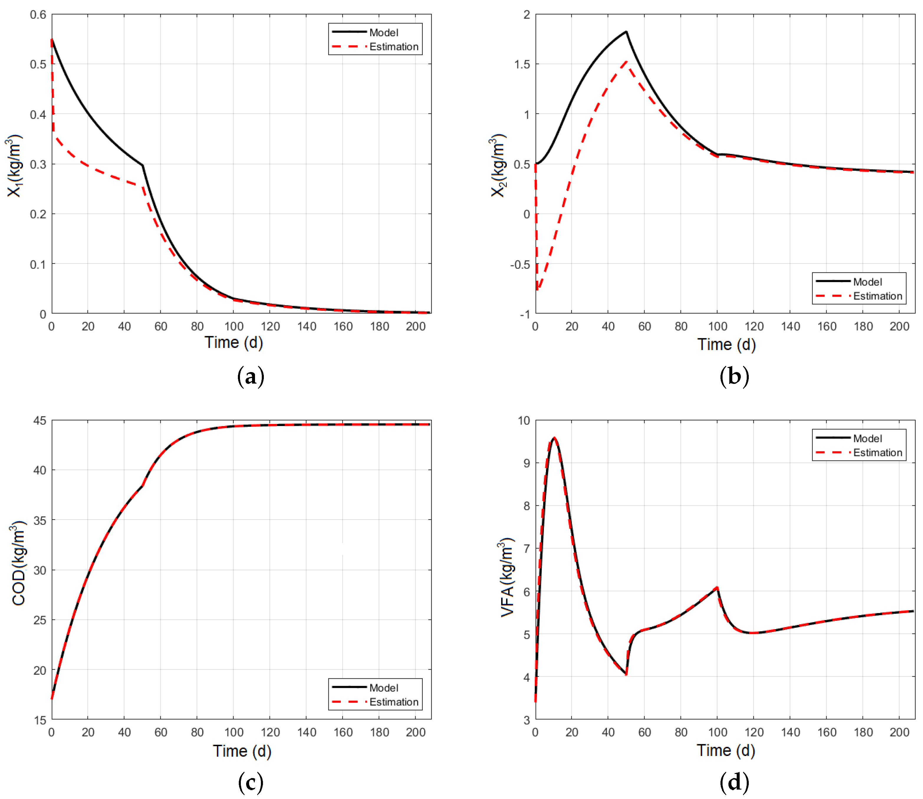
3.2. Asymptotic Estimator When Reaction Rates Are Unknown
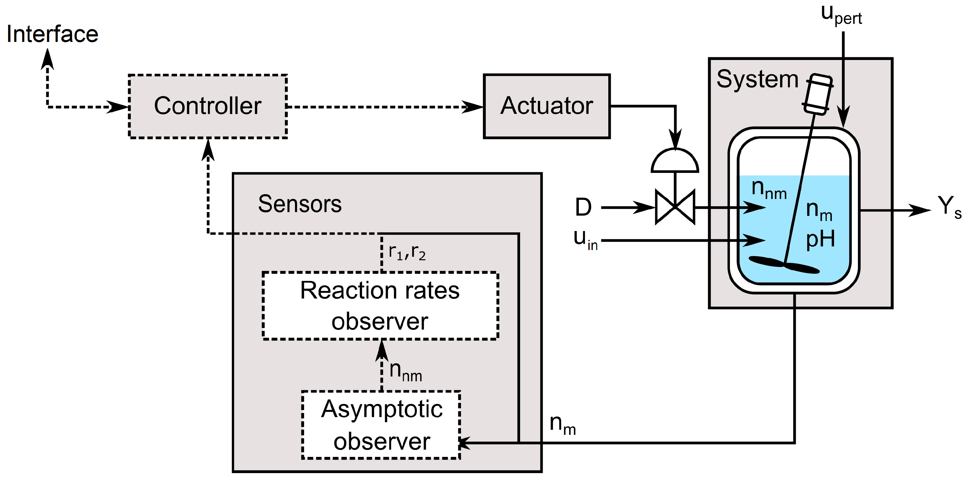
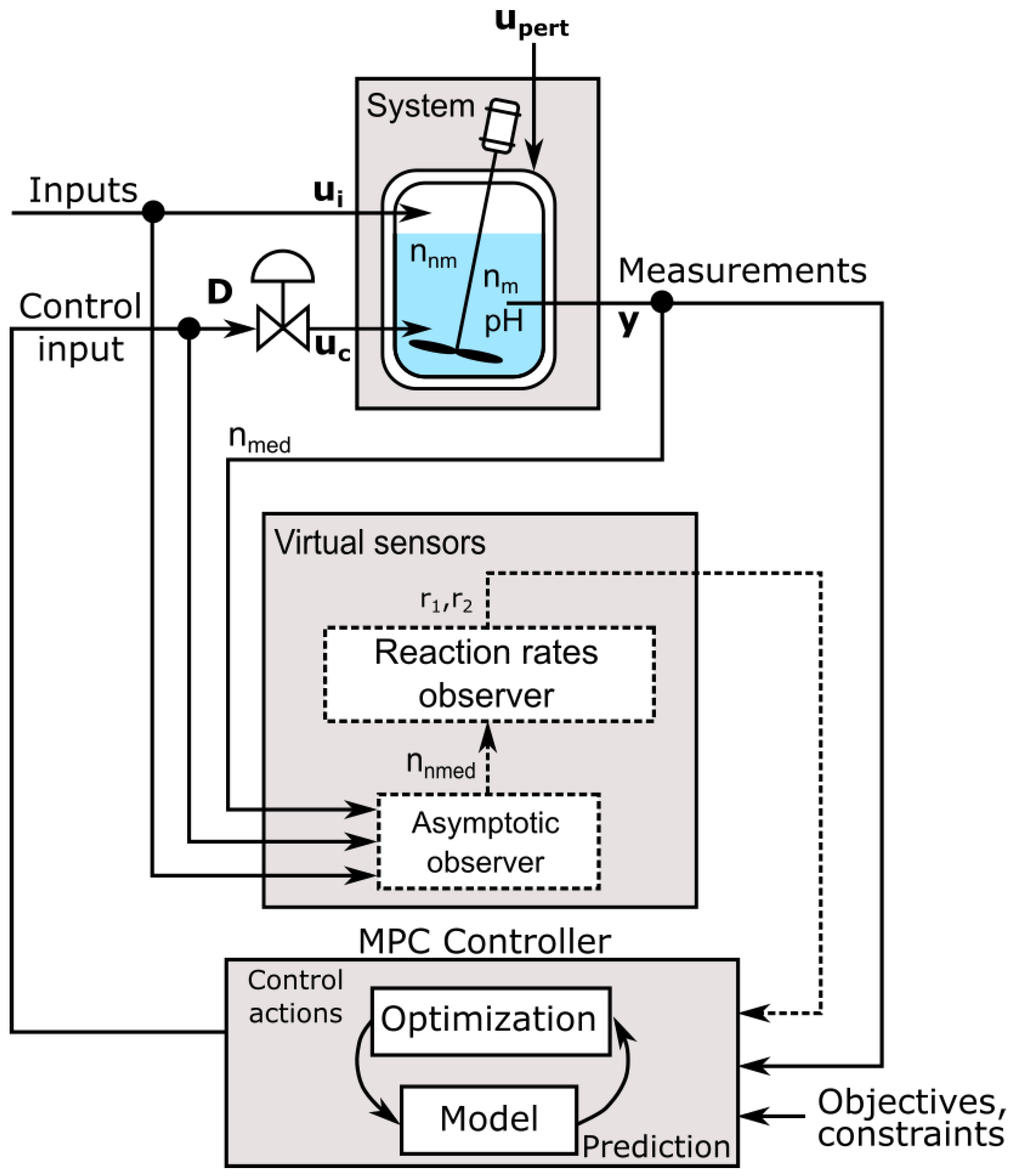
The absence of information due to the lack of reliable sensors or analysis results opens up an opportunity to substitute the uncertainty by the design of software sensors. In anaerobic reactors, this technology estimates the concentration of acidogens and methanogens without the information of the reaction rates [11]. It results in a particular category of observer-denominated asymptotics, because two conditions support its operation; the system is still not exponentially observable, and the reaction kinetics are unknown [14]. The detailed information of the design is presented in Cortés et al. [13].
In the following, we present the conditions that affect the design of the algorithm: the information of the matrix ϕ is unknown, the yield coefficients from K are fully known, and the number of q state , the number of measured state variables, is the same or higher than the rank of the matrix K (that is, q s t a t e = dim( ξ 1 )   rank(K)). Hence, based on the previous information, the general equation of homogeneous reaction systems described by a general nonlinear state space model is presented:
d ξ d t = K ϕ ( ξ , t ) D ξ Q ( ξ ) + F
where dim( ξ ) = dim(F) = dim(Q) = N, dim( ϕ ) = M and dim(K) = N × M. Thus, the general nonlinear model Equation (12) can be divided as
d ξ a d t = K a ϕ ( ξ a , ξ b ) D ξ a Q a + F a
d ξ b d t = K b ϕ ( ξ a , ξ b ) D ξ b Q b + F b
where the rank of K is p. The submatrix K a results from a section of K with p × M. The submatrix K b has the remaining information of K. Finally, the matrices ( ξ a , ξ b ) , ( Q a , Q b ), and (F a , F b ) are the corresponding parts of ξ , Q, and F caused by the influence of K a and K b . The previous formulation has the following feature:
Z o b = A 0 ξ a + ξ b
There exists a transformation that considers Z o b as a linear combination of ξ a and ξ b as seen in Equation (15). Finally, after processing Equations (13)–(15), the new state space model is equivalent to:
d ξ a d t = K a ϕ ( ξ a , ξ b ) D ξ a Q a + F a
d Z o b d t = D Z o b + A 0 ( F a Q a ) + ( F b Q b )
The expression F a Q a = 0 means the partition made by Equations (13) and (14) are appropriate since the new dynamics on Z o b are independent from K and ϕ . In Equation (16), the independence of ξ a ˙ from ϕ is stated. To extend for detailed information, check the complete demonstration in Cortés et al. [13].

Observer Design

Using the nonlinear EAM2, the following equations describe the decoupled subsystem conducted by the state variables X 1 , X 2 , S 1 , and S 2 :
ξ = X 1 X 2 S 1 S 2 , F = 0 0 D S 1 i n D S 2 i n , Q = 0 0 0 0 , K = 1 0 0 1 k 1 0 k 2 k 3 , ϕ = μ 1 X 1 μ 2 X 2
Considering the previous subsystem, the subsequent state equation is structured as follows:
d d t X 1 X 2 S 1 S 2 = 1 0 0 1 k 1 0 k 2 k 3 ϕ 1 ϕ 2 D X 1 X 2 S 1 S 2 + 0 0 D S 1 i n D S 2 i n
where ξ a and ξ b group the measurable and non-measurable states, respectively. Thus, using the equations described in Cortés et al. [13], the expression of Z o b is as follows:
d Z o b d t = D Z o b + A 0 ( F a Q a ) + ( F b Q b )
where the matrices related to the equation are:
ξ b = X 1 X 2 , Z o b = Z o b 1 Z o b 2 , A 0 = 1 k 1 0 k 2 k 1 k 3 1 k 3 , ξ a = S 1 S 2
F a = D S 1 i n D S 2 i n , F b = 0 0
with:
Z o b = Z o b 1 Z o b 2 = A 0 ξ a + ξ b = 1 k 1 0 k 2 k 1 k 3 1 k 3 S 1 S 2 + X 1 X 2

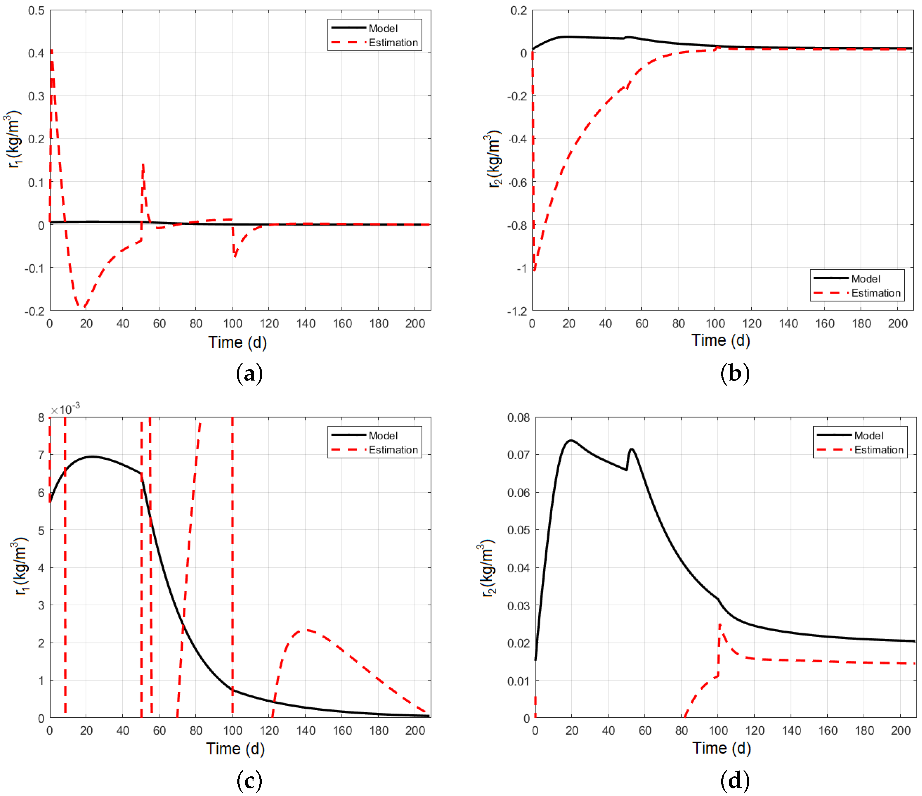
3.3. Kinetic Parameter Reaction Estimator

This section presents an additional tool that complements the lack of measurements in the reactor. The goal is to estimate the kinetic reactions coming from the reaction system. Figure 1 shows the structure proposed to obtain all the information needed to feed the mathematical model contained in the control scheme strategy.
The discontinuous line represents the information generated by the observers. At the end, the measured variables n m and the estimated ones converge to feed the controller algorithm. In order to design the kinetic estimator algorithm, the following nonlinear equation that represents the system must be considered:
ξ ˙ = K ϕ D ϕ Q + F
Equation (24) assumes that the coefficients from K are known, while the dilution rate D, the input flows F, and the gas output flows Q are measured in real-time. Additionally, it is assumed that ξ is fully-known because the non-measured dynamics are reconstructed by the previous asymptotic observer. The vector ϕ is partially known and is divided as follows:
ϕ = H ρ
The matrix H contains the information from the known kinetic reactions, and ρ contains the remaining information, the unknown kinetic reactions. Thus, using Equation (25) in Equation (24) results in Equation (26).
ξ ˙ = K H ρ D ϕ Q + F
The estimation of reaction kinetics, r 1 and r 2 , is equivalent to estimating the entire vector ρ . Hence, following the structure proposed by Bastin et al. [14], a new dynamic of the system is presented as follows:
ξ ^ ˙ = K H ρ ^ D ξ Q + F Ω ( ξ ξ ^ ) ,
ρ ^ ˙ = ( K H ) T Γ ( ξ ξ ^ )
where ρ ^ represents the real-time estimation of ρ . When ξ ξ ^ 0 occurs in Equation (28), it means that ρ ^ ˙ 0 results in a perfect tendency process of convergence to desirable reaction kinetics values ρ ^ ρ . There is a mandatory condition. Equation (27) that represents the kinetic reaction estimator has an equivalent structure to the Luenberger observer used in homogeneous reaction systems [14].
ξ ^ ˙ = A ξ ^ + B u 1 * + Ω ( ξ ξ ^ )
The underlined term 1 * in Equation (29), A ξ ^ + Bu, is equivalent to the term KH ρ ^ D ξ Q + F in Equation (27). Thus, the above-mentioned comparison results in Equation (30):
ξ ^ ˙ = K H ρ ^ D ξ Q + F 1 * Ω ( ξ ξ ^ )
In this way, Equation (30) represents the nonlinear system, while Equation (29) is the equivalent linearized system.

Observer Design

To design the kinetic reaction estimator, only the measured and estimated states on ξ ˙ are needed, while the term ξ ξ ^ is used as a reference to monitor and follow the estimator’s performance. ξ ^ should converge to ξ as soon as possible ( ξ ξ ^ ). The dynamics of ξ ˙ ^ depends on the evolution of the dynamics of the error e ˙ = (A Ω L)e. Thus, the references (the known values) that assist in tuning the kinetic reaction estimator are ξ , ξ ^ , K, and H. For better understanding, the following definitions are proposed: the term e = ξ ξ ^ means the observation error, and the term ρ ˜ = ρ ρ ^ means the tracking error. Hence, using Equations (31) and (32):
ξ ^ ˙ = K H ρ ^ D ξ Q + F Ω ( ξ ξ ^ )
ξ ˙ = K ϕ D ξ Q + F
Deriving on both sides of e and ρ ˜ , it results in e ˙ = ξ ˙ ξ ^ ˙ and ρ ˜ ˙ = ρ ˙ ρ ^ ˙ . Taking Equations (31) and (32) and replacing them by e ˙ results in:
e ˙ = K ϕ D ξ Q + F K H ρ ^ + D ξ + Q F + Ω ( ξ ξ ^ )
e ˙ = K ϕ K H ρ ^ + Ω e
e ˙ = K H ρ K H ρ ^ + Ω e
e ˙ = K H ( ρ ρ ^ ) + Ω e
e ˙ = K H ρ ˜ + Ω e
In the same way, the dynamic of the tracking error is as follows:
ρ ˜ ˙ = ( K H ) T Γ e + d ρ d t
Merging Equations (37) and (38) results in the following dynamic system:
e ˙ ρ ˜ ˙ = K H ρ ˜ + Ω e ( K H ) T Γ e + d ρ d t
Thus, after organizing the previous equation, it results in the following system:
e ˙ ρ ˜ ˙ = Ω K H H T K T Γ 0 e ρ ˜ + 0 d ρ d t
Replacing the matrices:
A = Ω K H H T K T Γ 0
V = 0 d ρ d t
This results in:
e ˙ ρ ˜ ˙ = A e ρ ˜ + V
According to the information described, the estimation procedure is performed as follows:
K a = k 1 0 k 2 k 3 , K b = 1 0 0 1 , F a = D S 1 i n D S 2 i n , F b = 0 0
The next step is to calculate the matrix A 0 ; thus, it means that:
A 0 = K b K a 1
In the following equations, the system is divided into the dynamic states to be estimated, using the data from the asymptotic observer, Z 1 and Z 2 , and the measured data S 1 and S 2 . Solving ξ b from Equation (15), we obtain:
ξ b = Z o b A 0 ξ a
Equation (46) allows to calculate the following matrices:
K = K b K a , H = 1 0 0 1 , ξ = ξ b S 1 S 2 , F = F b F a
Finally, all the information needed to supply Equations (27) and (28) are obtained above.

4. Nonlinear Model Predictive Controller (Mpc)

As it is shown in Figure 1, the observer structure calculates the non-measurable dynamic states, the concentrations of X 1 and X 2 (with the asymptotic observer), and the kinetic reaction rates r 1 and r 2 (with the reaction rate observer). Once the information from measurements and virtual sensors has been delivered to the controller, the algorithm is ready to start calculating the control actions after receiving the rest of the information: the operational and physical instructions, as well as the control objectives.

4.1. Controller Design

The subsequent conditions emerge as the required rules to take into consideration to design the controller.
  • The reactor has to be balanced to react against perturbations, always working within the physical and operational boundaries.
  • Methane production needs to be maximized all the time.
  • The environmental regulations and the capacity of the reactor to reduce the concentration of substrates at the inlet, S 1 and S 2 , conditioned the programming. Therefore, the rule S 1 (t) + S 2 (t) ≤ Kt d , where Kt d denotes the maximum effluent concentration of the both substrates considered, has to be followed.
  • The reactor has to be protected against failures due to unexpected high variations on VFA, and in consequence, inhibitions on the metabolism of microorganisms. Thus, an alternative is to use alkalinity as a base to neutralize the level of acids.
    S 2 ( t ) Z ( t ) = λ
Equation (48) tries to preserve a relation between VFA and Z during the operation of the reactor. According to the literature, λ has to be within 0.1 and 0.3, to maintain the microorganisms in a zone of comfort in regard to the level of acids [11].

4.2. Structure of the Controller

Finally, the structure of the controller is shown in Figure 2. The dilution rate D controls the amount of substrate at the inlet. It results in u C , the variables used by the MPC to manipulate the dynamics of the reactor. u i represents the non-controller variables considered as inlet: S 1 i n , S 2 i n , C i n , and Z i n . u p e r t holds the information about the inputs considered as disturbances. y contains the information of the variables available to be measured. n m are the state dynamics that can be measured: S 1 , S 2 , Z, and C. The value of pH is measured directly from the reactor. n n m are the state dynamics that cannot be measured directly from the reactor: X 1 and X 2 . The algorithm Virtual sensors allocates the two observers that estimate the variables n n m and the reaction rates r 1 and r 2 . The Asymptotic observer uses the information from y, u i , and D in the absence of the reaction rates. At the same time, n nm is used by the Reaction rate observer to calculate the reaction rates r 1 and r 2 . All the previous information is inserted into the MPC. Finally, the instructions about the objectives and constraints are detailed in Equation (49) [5].
We consider the mathematical model x ( k + 1 ) = f ( x ( k ) , u ( k ) ) described in Section 2.1. x ( k ) ϵ R n and u ( k ) ϵ R m are the state and input matrices, respectively, of the dynamical system at step-time k. f(·) is the nonlinear function that describes the dynamic system to be controlled.
max u ( k ) , , u ( k + N c ) J ( x ( k ) , u ( k ) ) subject to : x ( k + 1 ) = f ( x ( k ) , u ( k ) ) , y ( k ) = g ( x ( k ) , u ( k ) ) , x m i n x ( k ) , k = 1 , , N p , u m i n u ( k ) u m a x , k = 1 , , N u , S 2 ( k ) Z ( k ) λ , k = 1 , , N p
where J(·), x ( k ) , u ( k ) , y ( k ) , and g(·) are the functional cost that contains the information of the control objectives, the dynamics of the system, the controller inputs, the output function, and the function of the output, respectively [33]. x m i n represents the lower boundaries of the dynamics states. u m i n and u m a x are the lower and upper boundary limits of the control action, the dilution rate. The last condition is the buffer capacity, the indicator that quantifies the capacity reserved by the reactor to resist the acidity level. The dilution rate D can reach values from 0 to 1. Equation (50) shows the functional cost proposed, i.e., the total sum, along the simulation, of the volume of methane produced every day by the anaerobic reactor.
J ( x ˜ ( k ) , u ˜ ( k ) ) = h = k k + N P 1 X 2 ( h + 1 | k ) μ 2 ( h + 1 | k ) k 6
where X 2 ( h | k ) represents the predicted values of the acidogenic bacteria. μ 2 ( h | k ) has implicitly the value of the dynamic of VFA S 2 ( h | k ) (see Equation (4)). h represents the current time at time step k. u ( h ) denotes the control input D. x ˜ ( k ) = [x T ( k + 1 | k ) , ⋯, x T (k + N P | k )] T , and u ˜ ( k ) = [u T ( k + 1 | k ) , ⋯, u T (k + N P | k )] T , where x ( k | k ) = x ( k ) , and u ( h ) = u(k + N C − 1), for h = k + N C , ⋯, k + N P − 1. N C and N P are, respectively, the control and prediction horizons, where N C N P . According to the above-mentioned, x ˜ ( k ) and u ˜ ( k ) are the predictions of the states and input matrices over the time horizon N P . Two step changes in the profile inputs are considered to test the performance of the proposed MPC. The changes at the inlet simulate an unexpected overload trying to drive the system closer to the operational limits [11]. The simulations performed have been meticulously selected in agreement to a sufficiently range of operating conditions. The focus is to inspect the control actions calculated trying to preserve the operation under the limits. Two MPC are programmed to run without any operational restrictions. One of them, used as a reference, is programmed to run without the multistart function (a mesh of random points that start the solver from multiple points to find multiple local minima), while a second MPC, with the same characteristics as the previous, operates with the multistart function. Two additional MPCs are configured to operate under the same conditions but with operational restrictions. In this way, the progress of the system operating under stressful situations can be checked. An industrial PID controller is used to analyze, compare, and discuss the performance of the MPC schemes proposed [34].

5. Simulation Results and Analysis

Let us consider a system such as the reactor shown in Figure 2. Numerous simulations are performed to validate the methods suggested in this paper. The control horizon N C and the predictive horizon N P of the MPC are set to 5 and 7 days, respectively. The values of S 1 i n , S 2 i n , and Z i n are the same as the ones used in Cortés et al. [13]. The machine used to perform the simulations has the following specifications: Intel® Core™ i7-1165G7 processor (12 MB Cache). RAM memory 8 GB (1 × 8 GB) DDR 4 3200 MHz. Storage capacity SSD 512 GB CL35 M.2. Graphics NVIDIA® GeForce® MX 330 2 GB GDDR 5.
The reaction rates (considered as static in previous works [11]) changed over time, are calculated from the Reaction rate observer [10]. In addition, this section evaluates the performance of both configurations; the Asymptotic observer that estimates the concentrations of acidogens and methanogens, and the reaction rate observer that estimates the two kinetic reactions used at EAM2. In a second stage, with the observers under operation connected to the controller, the performance of the MPC is tested using four different configurations. This section employs the same profile inputs and the initial conditions used in the parametric identification procedure detailed in Cortés et al. [13].

5.1. Asymptotic Observer

This category of observers is named asymptotic because it estimates the non-existing measurable states based on two conditions; the system is still not exponentially observable, and the reaction kinetics are unknown [14]. To overpass the lack of information needed by the controller, the first step is checking the operation of the observer that estimates X 1 and X 2 .
The results obtained by the algorithm are complied elsewhere [13]. To test the observer’s performance, the starting point of both simulations, the observer and the dynamical model, were set on different values in order to confirm the convergence [13].

5.2. Kinetic Parameter Reaction Estimator

The good results obtained from the Asymptotic observer far exceed the minimum standard requirements needed for its use. Now, to unlock the calculus of the kinetic reaction rates (r 1 and r 2 ), the information of the previous estimations are all inserted with the measurements of the states n m and pH from the reactor [27,28]. In order to test the efficiency (and convergence) of the Reaction rate observer, the results are compared with the measurements held by the calculus of the same variables on EAM2 (see Figure 3a). Both simulations are subjected to the same changes in the profile inputs. From day 0 until day 50 of the simulation, the value of D is 0.03 d 1 . Then, from the day 51, D changed to 0.07 d 1 and maintained its value until day 100, when the last change situated D at 0.05 d 1 .
Due to a difference in scale magnitude, it is not possible to closely follow the process of convergence. Hence, Figure 3c,d shows a zoom, focusing the view on the step changes and the processes of convergence. The results of the state dynamic observer are shown in Figure 4. Despite the values of the dynamic observer started from different points, the process of convergence shows successful results after 100 days. As expected, the dynamic states S 1 and S 2 from the observer are directly obtained by EAM2 following the same results.

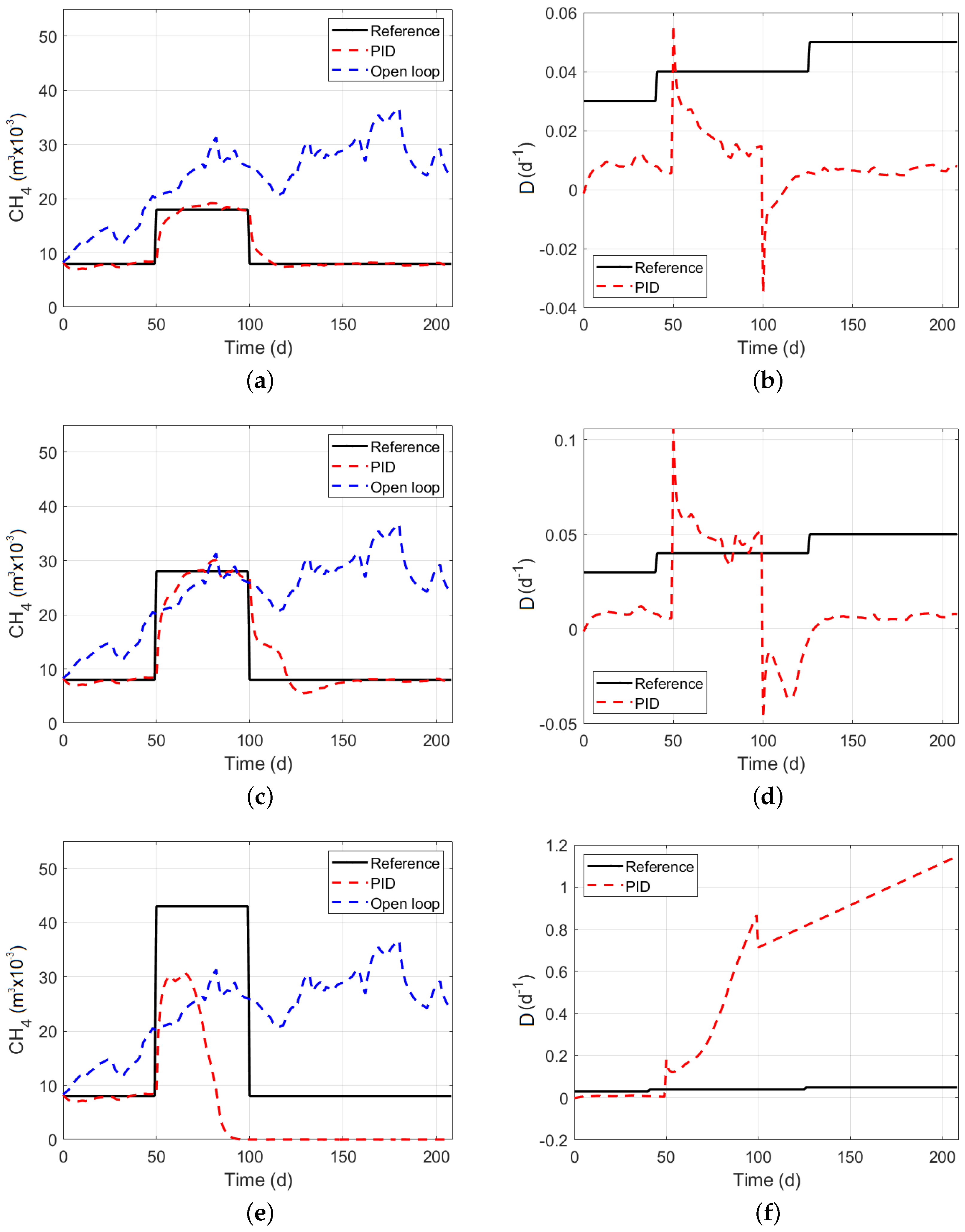
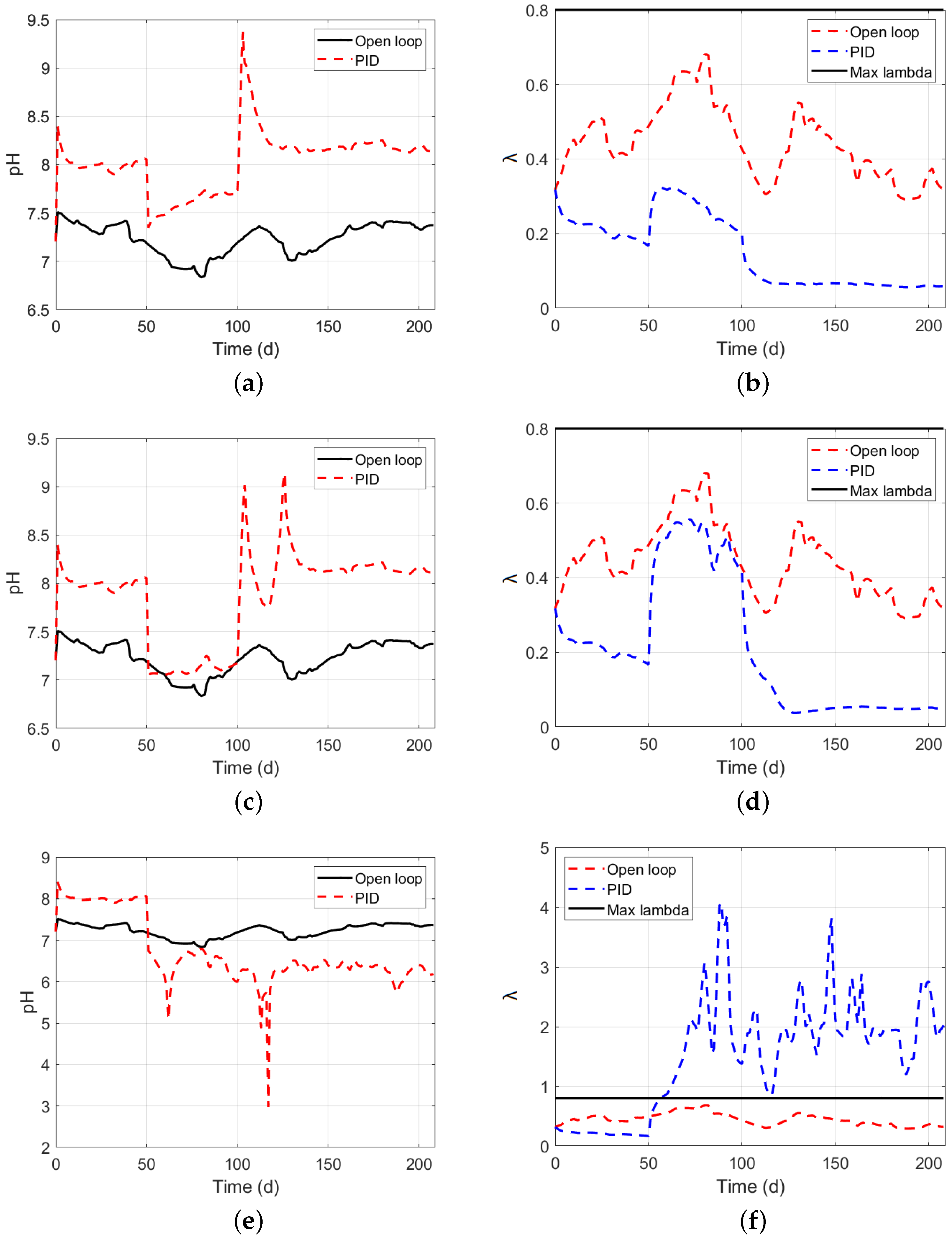
5.3. Pid Controller Performance on Anerobic Digesters

This section explores the performance of the PID controller used in the anaerobic reactor, aiming to establish a coherence in a comparative analysis between the control strategies studied. The simplicity of its controller is used to evaluate the decisions taken from the four MPC configurations. The main difference is that the PID controller reacts in correspondence to the current situation sensed from the reactor, while the MPC calculates the control actions aiming to maximize the methane produced. The algorithm used by the MPC has the information of the physical and operational restrictions that conditioned the calculus of the control actions.
Three different scenarios are performed by the PID controller to follow the reference methane produced. Using step changes in a reference, the PID controller is evaluated in its capabilities to guide the production under feasible scenarios. The PID control scheme tests its robustness under moderate, medium, and extreme scenarios in the objective to produce methane (see Figure 5). The changes occurred at day 50 and remained constant until day 100. After that, the reference goes back to the previous value to check the controller’s capacity to be recovered (black line). The discontinuous blue line represents the methane production using the profile inputs in the parameter identification procedure, Cortés et al. [13]. The objective is to use these results as a reference to compare the different performances (discontinuous red line). Figure 5a,c shows the capacity for the controller to follow the reference in moderate and medium scenarios. Before day 50, the controller maintained its operation closer to the reference. However, when the references change to 18 × 10 3 m 3 /d and 28 × 10 3 m 3 /d, respectively, the controller shows the capacity to follow new requirements. Nevertheless, Figure 5e shows that the controller is not capable to follow the reference (when the values change up to 43 × 10 3 m 3 /d). The system falls into a destabilization region, where methane production dropped below even when the reference returned to the previous state. As expected, since the controller does not have information about the physical and operational restrictions, the system, under certain unfavorable condition scenarios, could operate outside the boundaries beyond permissible limits.
The correspondent values of dilution rate D over the three scenarios are shown in Figure 5b,d,f. Figure 5b,d shows a normal operation of D just before the day 100 when the system crashed because the value of D dropped below zero.
Once again, the values of pH linked to the PID controller operate beyond the right limits. The previous analysis induces to prepare and incorporate future strategies that contain the drawbacks associated with unusual values in λ , and in consequence, S 2 . Figure 6b,d,f, shows the value of λ along the simulation for the three correspondent cases. Below the limit recommended (0.8) by some authors in the literature [11], λ in the first two cases (Figure 6b,d) corresponds to correct values. However, when the limits are exceeded, see Figure 6f, the value of S 2 far exceeds the limits, resulting in values of λ closer to 4. As stated in previous results, the PID controller cannot manage the system within physical and operational boundaries. Based on previous results, the alternative proposed in this paper, the MPC controller, becomes a reasonable option because its algorithm considers valuable characteristics that help the system to preserve in order to maintain the microorganisms under feasible scenarios [18].

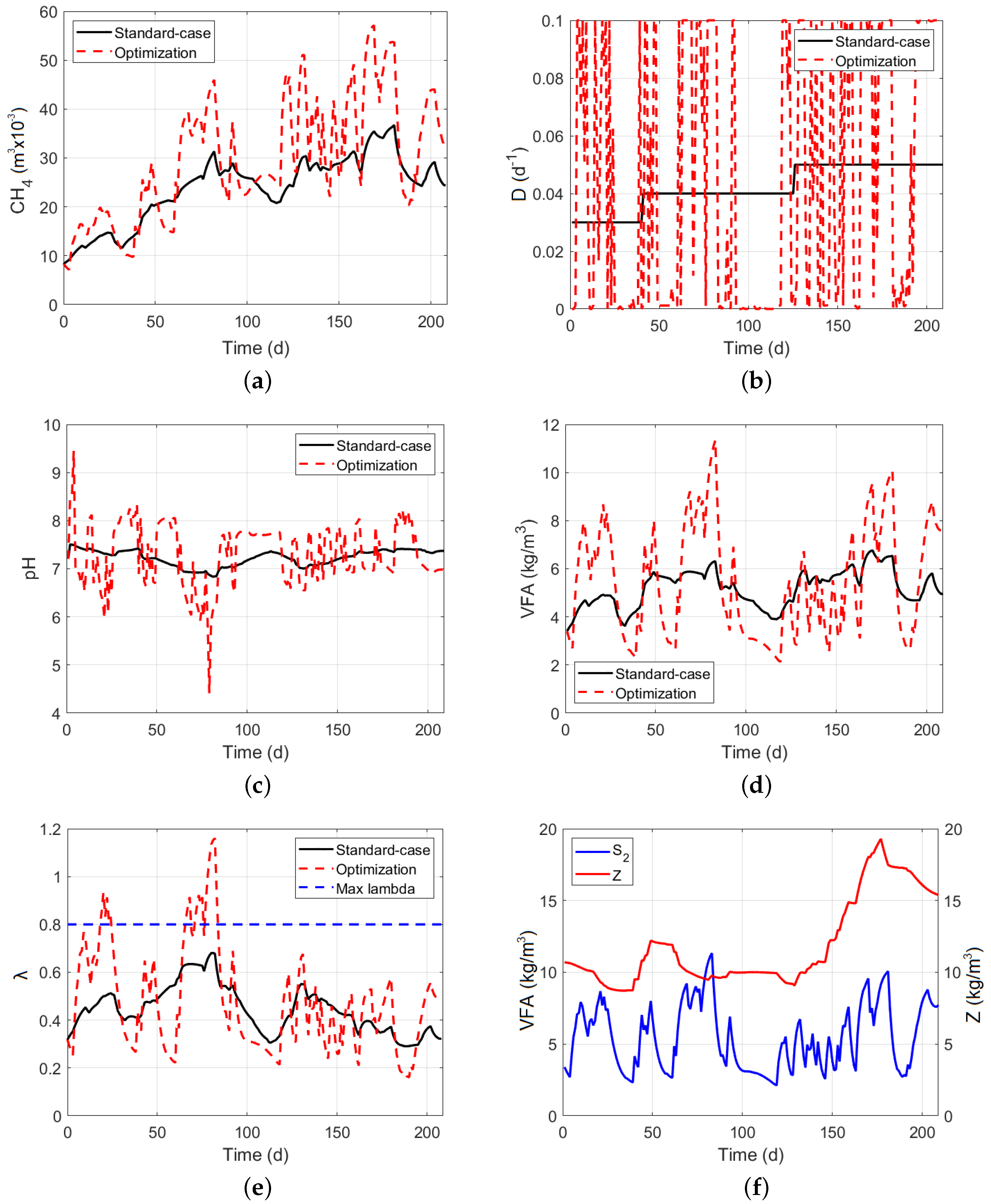
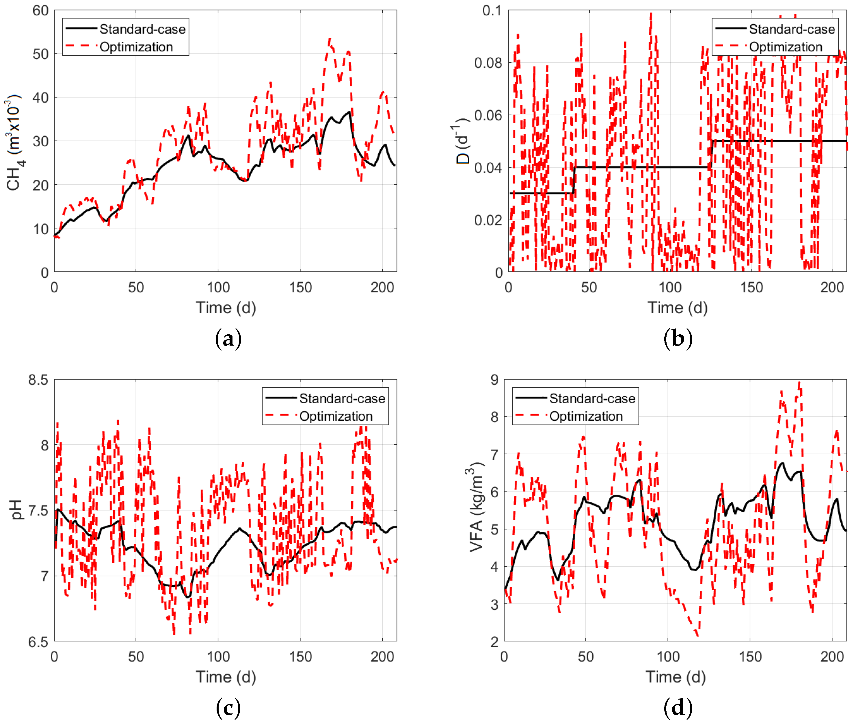
5.4. Mpc Controller without Restrictions

Figure 7 shows the results of maximizing the methane produced by the reactor using an MPC without the operational and physical restrictions shown in Equation (49).
Figure 7a shows a substantial increase in the volume of methane produced (see discontinuous red line), where the black line acts as the reference (volume of methane produced due to profile inputs used in parametric optimization), to measure the improvements on efficiency. The correspondent control actions calculated are shown in Figure 7b. The absence of restrictions in the algorithm allows the controller to calculate control actions, neglecting strong changes in operation that could affect the stability of the reactor. As can be seen, maximizing the objective turns the values of D extreme; showing oscillations from one extreme to the other. Several times the value of D decreases to zero and suddenly rise to the maximum. In the same way, pH had severe changes even beyond the operational limits (see Figure 7c). The relationship between pH and VFA is clear in Figure 7c,d showing a correlation along the simulation. This algorithm exposes high external risks in operation because there exists a lack of information over the system’s operation. Figure 7e shows the corresponding values of λ along the simulation; it appears that the values go beyond the limits repeatedly. As it seems in Figure 7f, the value of alkalinity Z exceeds the value of S 2 where at this point, the value of λ goes beyond 1, meaning the reaction system runs inadequately.
Given the previous results in Figure 7, the maximization of methane without restrictions leads the system to operate beyond non-feasible limits. Therefore, it is necessary to include extra information about the process to avoid inhibitors along the simulation.
Figure 8 shows the results obtained due to the operation of the MPC without the restriction of buffering capacity ( λ ) and without the multistart function. Figure 8a shows the volume of methane produced by both the reference (black line), and the MPC (red discontinuous line). A significant increase in the volume of methane produced compared to the reference is observed. Figure 8b shows the control actions calculated by the MPC. As it is shown, the oscillation is severe, however, the results are reliable. Figure 8c,d shows the results of the pH and S 2 . As expected, the oscillation of values is intense around the reference (black line) but not attractive for control purposes. Finally, Figure 8e shows the evolution of the non-restricted parameter λ . As expected, due to the absence of restrictions on programming, the maximum value of λ has been exceeded once.

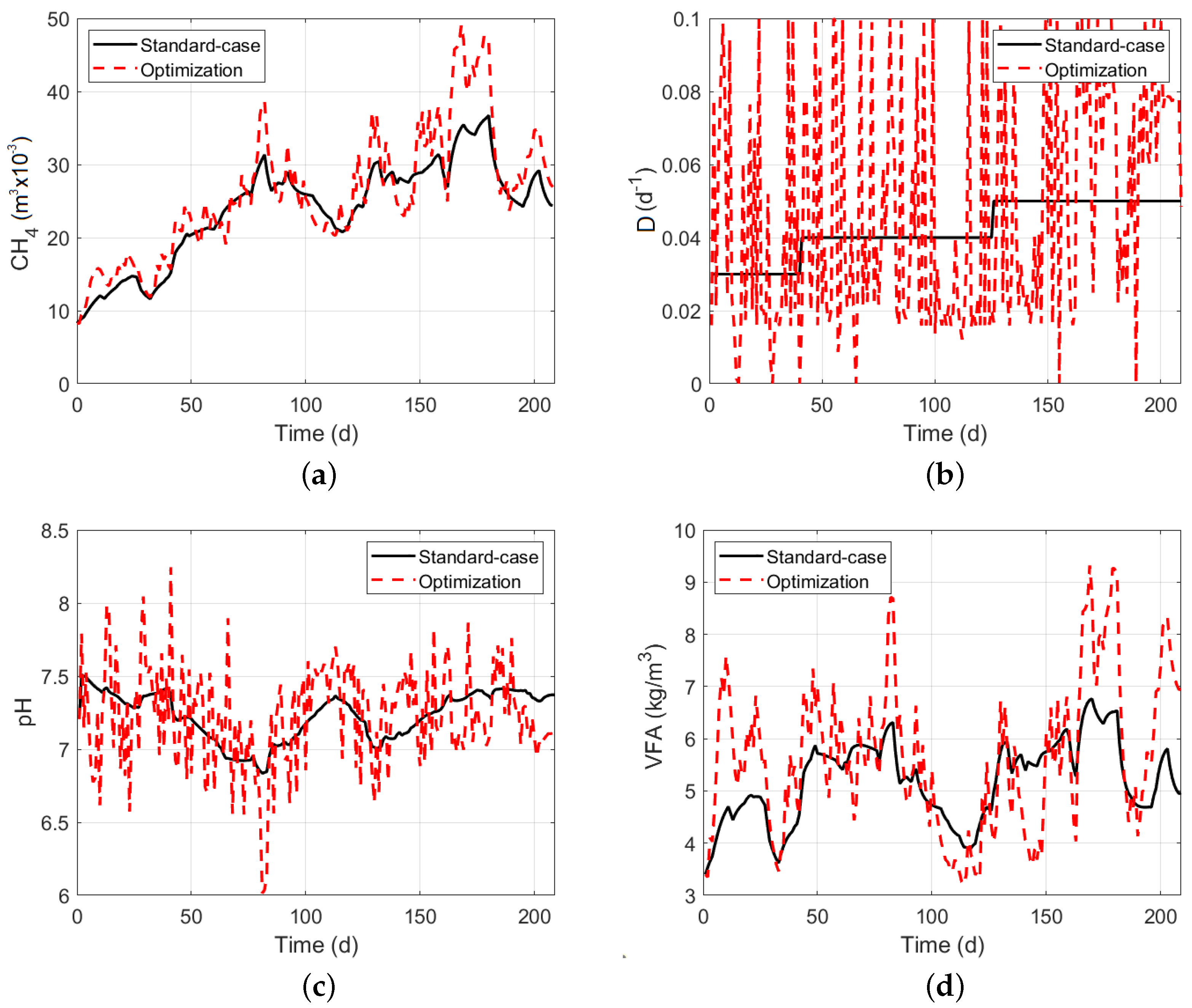
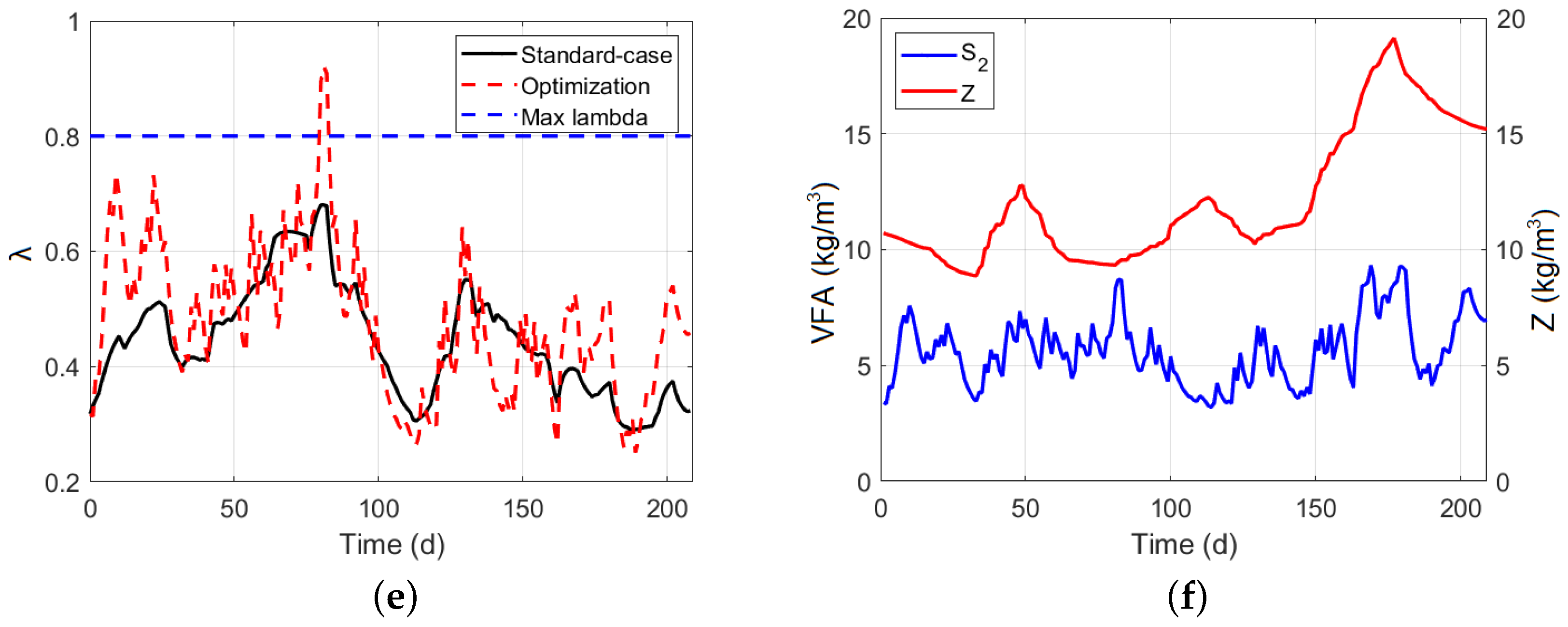
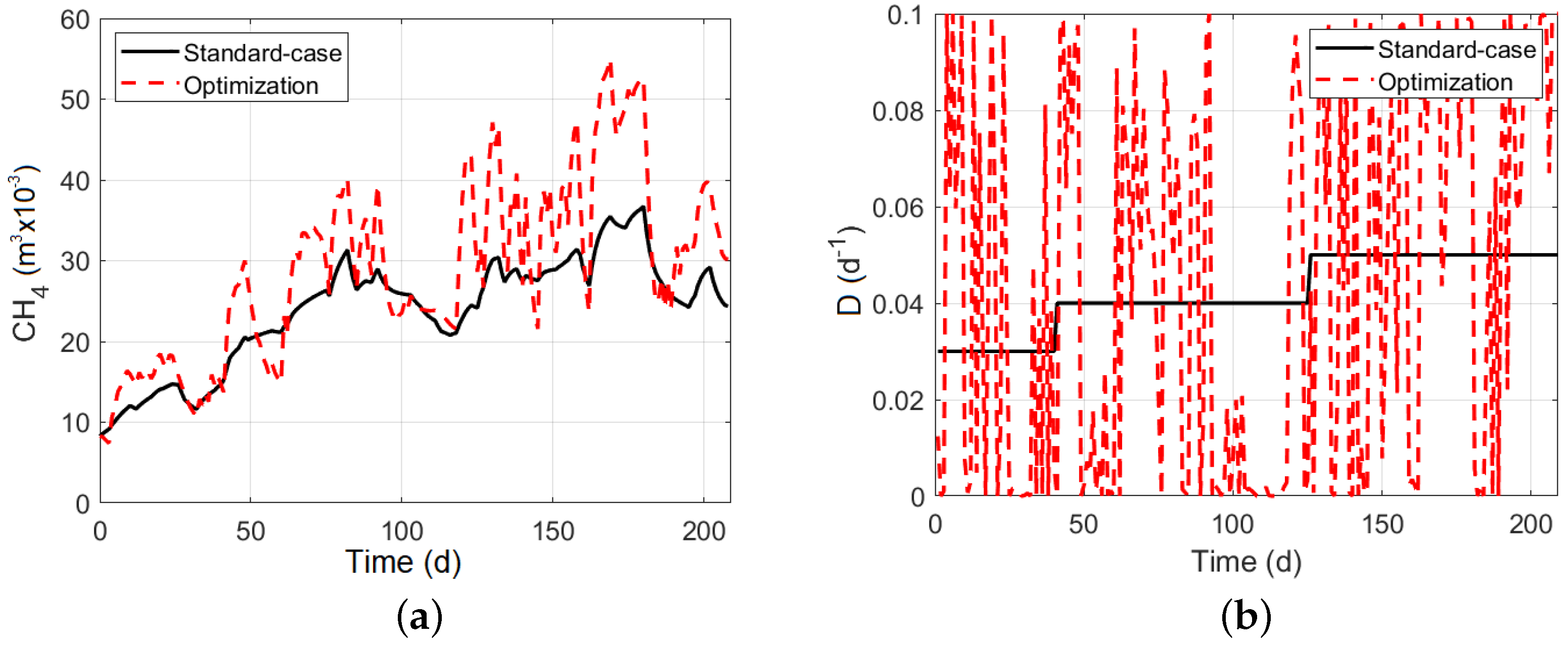
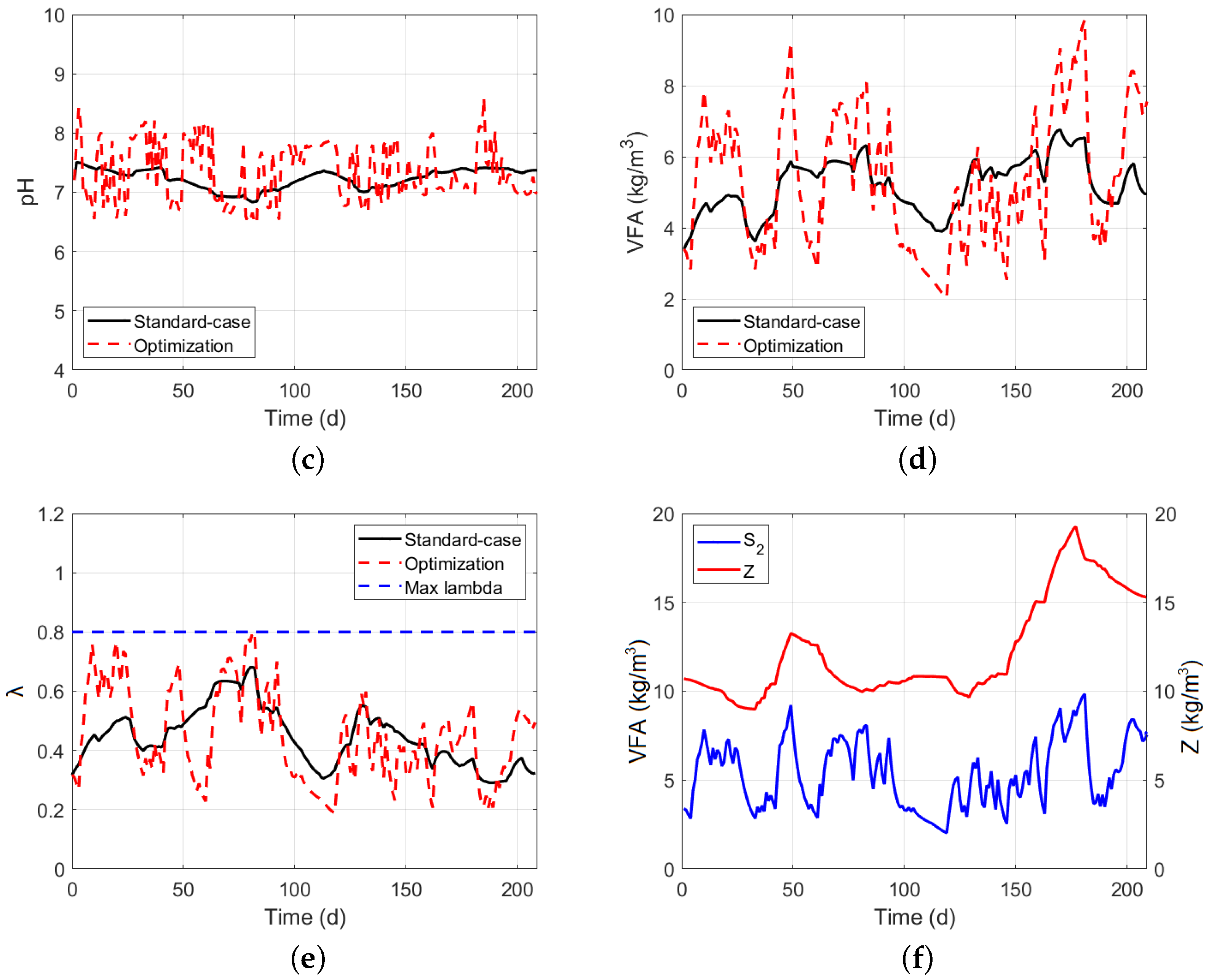
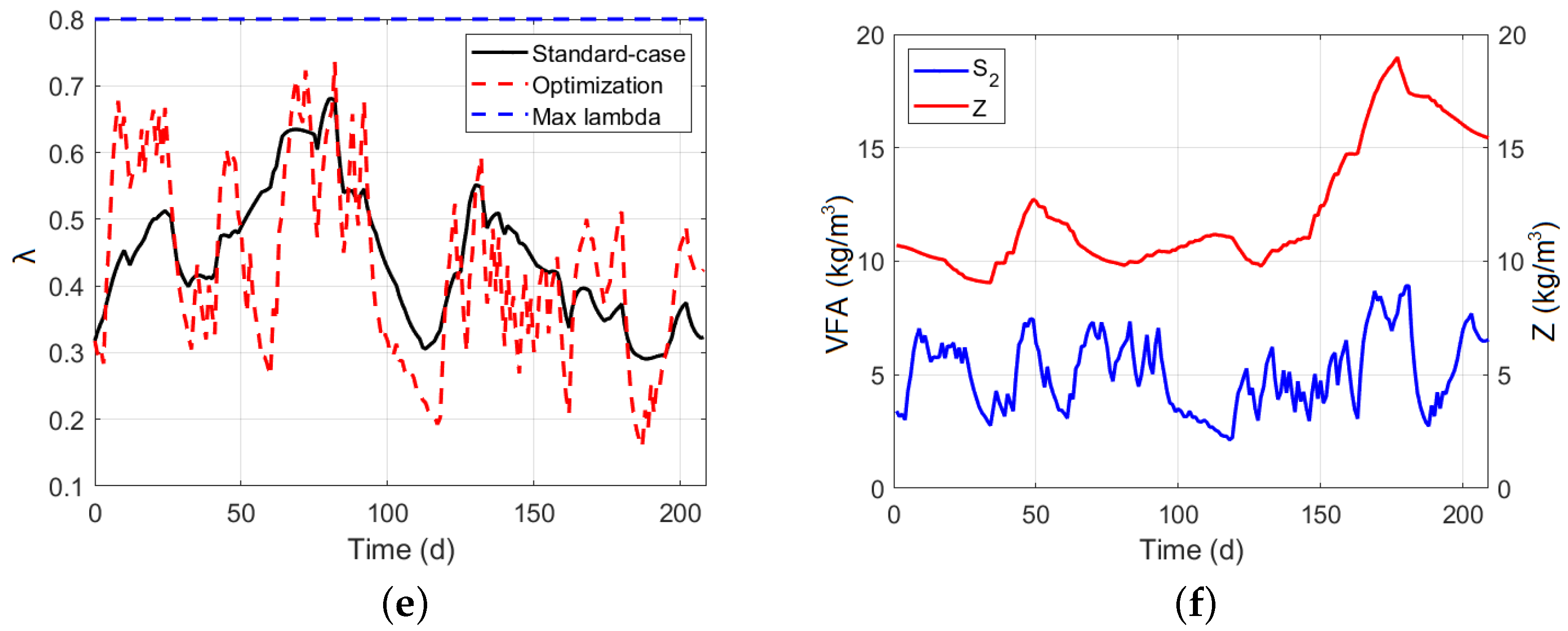
5.5. Model Predictive Controller with Restrictions

The information about operational and physical restrictions is added to the MPC aiming to maintain the microorganisms under feasible operational conditions. As shown in Figure 9a, the discontinuous red line shows the volume of methane produced. The efficiency is maintained despite the restrictions; therefore, this option better fits the system under stable conditions. The correspondent control actions calculated by the optimizer (see Figure 9b) shows a slight attenuation compared with previous simulations. The results of pH in Figure 9c show that the range of values becomes closer to the reference than the previous results. Compared with the previous results, the acidification level is much lower (see Figure 9d). In Figure 9e, the discontinuous blue line represents the limit stated for a regular operation. As it is shown, the discontinuous red line never surpasses the limits beyond λ = 0.8; in some cases, it gets closer. However, it is because the reactor is producing a high amount of methane closer to the operational limits. Figure 9f shows the evolution of the balance between VFA and Z. It is clear that the buffer capacity is always under control. Although the algorithm is restricted, the amount of methane CH 4 produced is higher than the reference.
Finally, Figure 10 shows similar results to those shown in Figure 8 but programmed without the multistart function. Despite the decrease in efficiency, the results show an adequate operation.
Table 1 shows a condensed vision of the previous results. Two same alternatives were simulated without the multistart function. As expected, there is a reduction in efficiency because the algorithm chose a random initial point to start the process. The black line is used as a reference to compare easily the results from the methane produced by the MPC [13]. In the case of the MPC controller that operates without operational restrictions, the improvement achieved was 17.4% and 24.4%, respectively, for the algorithm with no multistart and the multistart function.
The reactor that operates with operational restrictions shows an improvement of 18.8% and 20.8% for both MPC schemes, without and with the multistart function, respectively. Although the performance is reduced significantly because of the insertion of restrictions, the continuous operation of the reactor is not broken and can run permanently.

6. Conclusions

A structure of two observers demonstrates to be effectively solving two specific drawbacks responsible for the inefficiencies implementing control schemes based on modeling. The Asymptotic observer that operates in the absence of the reaction rates demonstrates an error of convergence less than 5% estimating the concentrations of acidogens and methanogens. Then, the previous information enables an upstream operation feeding the kinetic observer that estimates the reaction rates with an error of convergence lower than 5%. In the following, the rest of the parameters, considered as static due to their correlation with the specific biochemical characteristics of the organic matter, were calculated using algorithms based on optimization. All the above-mentioned aspects represent the key that makes it possible to operate MPCs in the industry. Four MPC configurations were used to test the observer and identification structure proposed. The objective was to maximize the volume of methane. While the controller without the operational restrictions showed a considerable increase in efficiency, after operational limits were added to the algorithm, the efficiency of the controller slightly decreased. However, its reduction on efficiency is affordable because the algorithm helped the system to stay in operation continuously. Without operational restrictions, the efficiency reached 24.4%, while the restricted algorithm showed an efficiency of 20.9%. The exhaustiveness in the methodology proposed is worth using because the added information guarantees robustness in operation and an increase in efficiency compared with traditional control alternatives.

Author Contributions

Conceptualization, L.G.C., J.B., D.F.L., J.D.M.-B., C.P. and M.A.d.l.R.; Data curation, L.G.C., C.P. and M.A.d.l.R.; Formal analysis, D.F.L., J.D.M.-B., C.P. and M.A.d.l.R.; Investigation, L.G.C., J.B., D.F.L., J.D.M.-B., A.F.M., C.P. and M.A.d.l.R.; Methodology, L.G.C., J.B. and C.P.; Project administration, J.B. and C.P.; Resources, J.D.M.-B. and A.F.M.; Software, L.G.C.; Supervision, D.F.L., J.D.M.-B. and M.A.d.l.R.; Validation, D.F.L. and M.A.d.l.R.; Visualization, L.G.C.; Writing—original draft, L.G.C.; Writing—review & editing, J.B., D.F.L. and C.P. All authors have read and agreed to the published version of the manuscript.

Funding

The authors wish to express their gratitude to Fundación FIDETIA (G91045419), Universidad de Sevilla, Spain, for funding this work. The author Luis G. Cortés express special acknowledgements to Fundación Centro de Estudios Interdisciplinarios Básicos y Aplicados (CEIBA), Colombia, for funding. Laboratorio de Investigaciones en Catálisis y nuevos materiales LICATUC (Universidad de Cartagena).

Data Availability Statement

The initial experimental results developed in this study are in the next link: https://doi.org/10.1016/j.procbio.2005.03.073 (accessed on 20 August 2022).

Conflicts of Interest

The authors declare that they have no known competing financial interests or personal relationships that could have appeared to influence the work reported in this paper.

Nomenclature

C , C i n Total inorganic carbon concentration (kg/m 3 )
DDilution rate (d 1 )
k 1 Yield substrate degradation
k 2 Yield for VFA production
k 3 Yield for VFA consumption
k 4 Yield for CO 2 production
k 5 Yield for CO 2 production
k 6 Yield for CH 4 production (m 3 )
K S 1 Half-saturation constant (kg/m 3 )
K S 2 Half-saturation constant (kg/m 3 )
K Z , 1 Yield for ammonium production (kg/m 3 )
K Z , 2 Yield for ammonium production (kg/m 3 )
q C Carbon dioxide flow rate (m 3 /d)
q M Methane flow rate (m 3 /d)
r 1 , r 2 Reaction rates (d 1 )
S 1 , S 1 i n Organic substrate concentration (kg acid acetic/m 3 )
S 2 , S 2 i n Volatile fatty acids concentration (kg/m 3 )
X 1 Concentration of acidogenic bacteria (kg/m 3 )
X 2 Concentration of methanogenic bacteria (kg/m 3 )
Z , Z i n Total alkalinity (kg/m 3 )
α Fraction of bacteria in the liquid phase
μ 1 Specific growth rate of acidogenic bacteria (d 1 )
μ 2 Specific growth rate of methanogenic bacteria (d 1 )
ψ 1 Maximum acidogenic bacteria growth rate (d 1 )
ψ 2 Maximum methanogenic bacteria growth rate (d 1 )
n m Vector of measured state variables
n n m Vector of non-measurable state variables
p , p m a x Vector of parameters
u , u m i n , u m a x Control action (d 1 )
ξ Vector of state variables
KMatrix with the kinetics of the biochemical
ϕ Microbiological reactions involved on system
QGaseous rate of mass outflow from reactor
FMass feed rate due to external substrates
ρ Unknown functions of all states
HKnown functions of all the states
Γ Gain matrix of the updating law
Ω Square gain convergence matrix
λ Buffer capacity
N p Prediction horizon (d)
N u Control horizon (d)

References

  1. Singh, R.; Sahay, A.; Karry, K.M.; Muzzio, F.; Ierapetritou, M.; Ramachandran, R. Implementation of an advanced hybrid MPC–PID control system using PAT tools into a direct compaction continuous pharmaceutical tablet manufacturing pilot plant. Int. J. Pharm. 2014, 473, 38–54. [Google Scholar] [CrossRef] [PubMed]
  2. le Roux, J.; Olivier, L.; Naidoo, M.; Padhi, R.; Craig, I. Throughput and product quality control for a grinding mill circuit using non-linear MPC. J. Process Control 2016, 42, 35–50. [Google Scholar] [CrossRef] [Green Version]
  3. Corbett, B.; Macdonald, B.; Mhaskar, P. Model Predictive Quality Control of Polymethyl Methacrylate. IEEE Trans. Control Syst. Technol. 2015, 23, 687–692. [Google Scholar] [CrossRef]
  4. Lora Grando, R.; de Souza Antune, A.M.; da Fonseca, F.V.; Sánchez, A.; Barrena, R.; Font, X. Technology overview of biogas production in anaerobic digestion plants: A European evaluation of research and development. Renew. Sustain. Energy Rev. 2017, 80, 44–53. [Google Scholar] [CrossRef] [Green Version]
  5. Marquez-Ruiz, A.; Mendez-Blanco, C.; Porru, M.; Özkan, L. State and Parameter Estimation Based On Extent Transformations. Comput. Aided Chem. Eng. 2018, 44, 583–588. [Google Scholar]
  6. Gaida, D.; Wolf, C.; Bongards, M. Feed control of anaerobic digestion processes for renewable energy production: A review. Renew. Sustain. Energy Rev. 2017, 68, 869–875. [Google Scholar] [CrossRef]
  7. Association, E.B. EBA Statistical Report; European Biogas Association: Brussels, Belgium, 2017. [Google Scholar]
  8. Méndez-Acosta, H.; Palacios-Ruiz, B.; Alcaraz-González, V.; González-Álvarez, V.; García-Sandoval, J. A robust control scheme to improve the stability of anaerobic digestion processes. J. Process. Control 2010, 20, 375–383. [Google Scholar] [CrossRef]
  9. Anukam, A.; Mohammadi, A.; Naqvi, M.; Granström, K. A Review of the Chemistry of Anaerobic Digestion: Methods of Accelerating and Optimizing Process Efficiency. Processes 2019, 7, 504. [Google Scholar] [CrossRef] [Green Version]
  10. Bernard, O.; Hadj-Sadok, Z.; Dochain, D.; Genovesi, A.; Steyer, J. Dynamicals Model Development and Parameter Identification for an Anaerobic Wastewater Treatment Process. Biotechnol. Bioeng. 2001, 75, 424–438. [Google Scholar] [CrossRef]
  11. Kil, H.; Li, D.; Xi, Y.; Li, J. Model Predictive Control with On-line Model Identification for Anaerobic Digestion Processes. Biochem. Eng. J. 2017, 128, 63–75. [Google Scholar] [CrossRef]
  12. López Buriticá, K.; Trujillo, S.; Acosta-Medina, C.; Granada, D.H. Dynamical Analysis of a Continuous Stirred-Tank Reactor with the Formation of Biofilms for Wastewater Treatment. Math. Probl. Eng. 2015, 2015, 512404. [Google Scholar] [CrossRef]
  13. Cortés, L.G.; Barbancho, J.; Larios, D.F.; Marín-Batista, J.; Mohedano, A.F.; Portilla, C.; de la Rubia, M.A. Full-Scale Digesters: An Online Model Parameter Identification Strategy. Energies 2022, 15, 7685. [Google Scholar] [CrossRef]
  14. Bastin, G.; Dochain, D. On-line Estimation and Adaptive Control of Bioreactors. Process Meas. Control. 1990, 10, 707–723. [Google Scholar] [CrossRef]
  15. Das, S.; Pan, I.; Halder, K.; Das, S.; Gupta, A. LQR based improved discrete PID controller design via optimum selection of weighting matrices using fractional order integral performance index. Appl. Math. Model. 2013, 37, 4253–4268. [Google Scholar] [CrossRef]
  16. Mauky, E.; Weinrich, S.; Jacobi, H.; Naegele, H.J.; Liebetrau, J.; Nelles, M. Model Predictive Control for Demand-Driven Biogas Production in Full Scale. Chem. Eng. Technol. 2016, 39, 652–664. [Google Scholar] [CrossRef]
  17. González, A.; Adam, E.; Marchetti, J. Conditions for offset elimination in state space receding horizon controllers: A tutorial analysis. Chem. Eng. Process. Process Intensif. 2008, 47, 2184–2194. [Google Scholar] [CrossRef]
  18. Hanema, J.; Lazar, M.; Tóth, R. Tube-based LPV Constant Output Reference Tracking MPC with Error Bound. IFAC-Pap. 2017, 50, 8612–8617. [Google Scholar]
  19. Wang, Y.; Witarsa, F. Application of Contois, Tessier, and first-order kinetics for modeling and simulation of a composting decomposition process. Bioresour. Technol. 2016, 220, 384–393. [Google Scholar] [CrossRef]
  20. Andrews, J.F. A Mathematical Model for the Continuous Culture of Microorganisms Utilizing Inhibitory Substrates. Biotechnol. Bioeng. 1968, 10, 707–723. [Google Scholar] [CrossRef]
  21. Rossi, E.; Pecorini, I.; Ferrara, G.; Iannelli, R. Dry Anaerobic Digestion of the Organic Fraction of Municipal Solid Waste: Biogas Production Optimization by Reducing Ammonia Inhibition. Energies 2022, 15, 5515. [Google Scholar] [CrossRef]
  22. Haldane, J. Enzynmes; MIT Press: Cambridge, MA, USA, 1965; p. 184. [Google Scholar]
  23. Marquez-Ruiz, A.; Mendez-Blanco, C.; Ozcan, L. Constrained Control and Estimation of Homogeneous Reaction Systems Using Extent-Based Linear Parameter Varying Models. Ind. Eng. Chem. Res. 2020, 59, 2242–2251. [Google Scholar] [CrossRef]
  24. García-Diéguez, C.; Bernard, O.; Roca, E. Reducing the Anaerobic Digestion Model No. 1 for its application to an industrial wastewater treatment plant treating winery effluent wastewater. Bioresour. Technol. 2013, 132, 244–253. [Google Scholar] [CrossRef] [PubMed]
  25. Chaib Draa, K.; Zemouche, A.; Alma, M.; Voos, H.; Darouach, M. A discrete-time nonlinear state observer for the anaerobic digestion process. Int. J. Robust Nonlinear Control 2019, 29, 1279–1301. [Google Scholar] [CrossRef]
  26. Song, Y.J.; Oh, K.S.; Lee, B.; Pak, D.W.; Cha, J.H.; Park, J.G. Characteristics of Biogas Production from Organic Wastes Mixed at Optimal Ratios in an Anaerobic Co-Digestion Reactor. Energies 2021, 14, 6812. [Google Scholar] [CrossRef]
  27. Batstone, D.; Keller, J.; Newell, B.; Newland, M. Model Development and Full Scale Validation for Anaerobic Treatment of Protein and Tat Based Wastewater. Water Sci. Technol. 1997, 36, 423–431. [Google Scholar] [CrossRef]
  28. Isaza-Hurtado, J.; Botero-Castro, H.; Alvarez, H. Robust Estimation for LPV Systems in the Presence of Non-uniform Measurements. Automatica 2020, 115, 108901. [Google Scholar] [CrossRef]
  29. Meegoda, J.N.; Li, B.; Patel, K.; Wang, L.B. A Review of the Processes, Parameters, and Optimization of Anaerobic Digestion. Int. J. Environ. Res. Public Health 2018, 15, 2224. [Google Scholar] [CrossRef] [Green Version]
  30. Bora, B.J.; Dai Tran, T.; Prasad Shadangi, K.; Sharma, P.; Said, Z.; Kalita, P.; Buradi, A.; Nhanh Nguyen, V.; Niyas, H.; Tuan Pham, M.; et al. Improving combustion and emission characteristics of a biogas/biodiesel-powered dual-fuel diesel engine through trade-off analysis of operation parameters using response surface methodology. Sustain. Energy Technol. Assess. 2022, 53, 102455. [Google Scholar] [CrossRef]
  31. Condrachi, L.; Vilanova, R.; Meneses, M.; Barbu, M. Anaerobic Digestion Process Control Using a Data-Driven Internal Model Control Method. Energies 2021, 14, 6746. [Google Scholar] [CrossRef]
  32. de la Rubia, M.; Perez, M.; Romero, L.; Sales, D. Effect of Solids Retention Time (SRT) on Pilot Scale Anaerobic Thermophilic Sludge Digestion. Process Biochem. 2006, 41, 79–86. [Google Scholar] [CrossRef]
  33. Valencia, F.; López, J.D.; Núñez, A.; Portilla, C.; Cortes, L.G.; Espinosa, J.; Schutter, B.D. Congestion Management in Motorways and Urban Networks through a Bargaining-Game-Based Coordination Mechanism; Springer: Berlin/Heidelberg, Germany, 2015; pp. 1–40. [Google Scholar]
  34. Batstone, D.; Keller, J.; Angelidaki, I.; Kalyuzhnyi, S.; Pavlostathis, S.; Rozzi, A.; Sanders, W.; Siegrist, H.; Vavilin, V. Anaerobic Digestion Model No 1 (ADM1). Water Sci. Technol. 2002, 45, 65–73. [Google Scholar] [CrossRef] [PubMed]
Figure 1. The controller and the observer structure proposed for the anaerobic reactor.
Energies 15 08594 g001
Figure 2. Model Predictive Control structure for the anaerobic digester.
Energies 15 08594 g002
Figure 3. Process of convergence in the estimation of reaction rates. (a) Values of r 1 ; (b) values of r 2 ; (c) zoom in r 1 ; (d) zoom in r 2 .
Energies 15 08594 g003
Figure 4. Kinetic reaction estimator to state variables considered. (a) Acidogens concentration X 1 ; (b) methenogens concentration X 2 ; (c) chemical oxygen demand; (d) volatile fatty acids.
Energies 15 08594 g004
Figure 5. Performance of PID control after step changes. (a) Low change in CH 4 ; (b) D values after a low change in CH 4 ; (c) medium change in CH 4 ; (d) D values after a medium change in CH 4 ; (e) high change in CH 4 ; (f) D values after a high change in CH 4 .
Energies 15 08594 g005
Figure 6. Performance of PID controller after step changes. (a) pH values after a low change in CH 4 ; (b) λ values after a low change in CH 4 ; (c) pH values after a medium change in CH 4 ; (d) λ values after a medium change in CH 4 ; (e) pH values after a high change in CH 4 ; (f) λ values after a high change in CH 4 .
Energies 15 08594 g006
Figure 7. MPC controller without restrictions, maximizing the volume of CH 4 . Time course of (a) volume of CH 4 ; (b) dilution rate D; (c) value of pH; (d) dynamic of VFA; (e) values of λ ; (f) dynamics of S 2 and Z.
Energies 15 08594 g007
Figure 8. MPC controller without restrictions. (a) Volume of CH 4 ; (b) dilution rate D; (c) value of pH; (d) dynamic of VFA; (e) values of λ ; (f) dynamics of S 2 and Z.
Energies 15 08594 g008aEnergies 15 08594 g008b
Figure 9. MPC controller with restrictions, maximizing the volume of CH 4 . (a) Volume of CH 4 ; (b) dilution rate D; (c) value of pH; (d) dynamic of VFA; (e) values of λ ; (f) dynamics of S 2 and Z.
Energies 15 08594 g009aEnergies 15 08594 g009b
Figure 10. MPC controller with restrictions. (a) CH 4 evolution; (b) D values calculated by optimizer; (c) pH values; (d) VFA values; (e) λ over the process; (f) evolution of S 2 and Z.
Energies 15 08594 g010aEnergies 15 08594 g010b
Table 1. Improvement in the methane produced by each MPC control scheme.
SchemesWithout RestrictionsWith Restrictions
No MultistartMultistartNo MultistartMultistart
Increase on efficiency17.4 %24.4%18.8%20.9%
Publisher’s Note: MDPI stays neutral with regard to jurisdictional claims in published maps and institutional affiliations.

