Atmospheric Drivers of Wind Turbine Blade Leading Edge Erosion: Review and Recommendations for Future Research

Abstract

Leading edge erosion (LEE) of wind turbine blades causes decreased aerodynamic performance leading to lower power production and revenue and increased operations and maintenance costs. LEE is caused primarily by materials stresses when hydrometeors (rain and hail) impact on rotating blades. The kinetic energy transferred by these impacts is a function of the precipitation intensity, droplet size distributions (DSD), hydrometeor phase and the wind turbine rotational speed which in turn depends on the wind speed at hub-height. Hence, there is a need to better understand the hydrometeor properties and the joint probability distributions of precipitation and wind speeds at prospective and operating wind farms in order to quantify the potential for LEE and the financial efficacy of LEE mitigation measures. However, there are relatively few observational datasets of hydrometeor DSD available for such locations. Here, we analyze six observational datasets from spatially dispersed locations and compare them with existing literature and assumed DSD used in laboratory experiments of material fatigue. We show that the so-called Best DSD being recommended for use in whirling arm experiments does not represent the observational data. Neither does the Marshall Palmer approximation. We also use these data to derive and compare joint probability distributions of drivers of LEE; precipitation intensity (and phase) and wind speed. We further review and summarize observational metrologies for hydrometeor DSD, provide information regarding measurement uncertainty in the parameters of critical importance to kinetic energy transfer and closure of data sets from different instruments. A series of recommendations are made about research needed to evolve towards the required fidelity for a priori estimates of LEE potential.

1. Introduction

1.1. Wind Turbine Blade Leading Edge Erosion

Leading edge erosion (LEE) is an emerging issue in wind turbine blade reliability [1]. Erosion of the leading edge causes gradual degradation of aerodynamic performance resulting in loss of annual energy production (AEP) [2,3,4]. While there is uncertainty regarding the response relationship between the severity of LEE and AEP losses [4,5], roughening of the blade leading edge reduces aerodynamic performance at roughness heights of 0.1 mm or below [6]. Accordingly, wind turbine blade LEE is a substantial cause of maintenance costs [7]. Reports suggest “structural repair of a single wind blade can cost up to $30,000, and a new blade costs, on average, about $200,000” [8], both of which inflate the Levelized Cost of Energy (LCoE) from wind. Increasing evidence of blade LEE has spurred development of advanced methods for detection of LEE [8,9,10,11], and to replicate the process of LEE in the laboratory [12,13] or using numerical modeling [14,15,16]. As an example of the latter, the Springer model has been applied for assessing the material properties and combined with Minor’s rule to assess time to failure [17]. Preventative tools to reduce LEE via application of polymer tapes or coatings to the leading edge have also been developed [10,18,19,20,21,22]. However, application of these tapes can reduce aerodynamic efficiency and thus power production [23]. Further, the tapes/coatings themselves can also be subject to erosion by shockwaves caused by impacts from hydrometeors [24].

Performance of leading edge protection (LEP) systems are typically evaluated using accelerated rain erosion tests (RET) [25]. Whirling-arm test-rigs are designed to determine the surface impact resistance of blade coatings to hydrometeor collisions. Many studies employ such systems, sometimes with a staged approach to examine the mechanisms by which coating systems evolve during the experiment [26]. They are used to perform experiments wherein a blade section is rotated at high-speed and exposed to droplet bombardment [13]. Although this experimental procedure has been widely used, it is subject to some limitations. For example, concerns have been raised that they do not sample realistic droplet size, morphology and velocity spectra [27]. They also do not fully include the presence of co-stressors such as degradation due to ultraviolet (UV) exposure or thermal cycling and associated materials expansion and contraction. Further, there is evidence that pre-stress of blade materials enhances hydrometeor erosion of the leading edge [28]. This effect is not fully reproduced in the whirling-arm test-rigs. Finally, current experimental configurations are limited to consideration of liquid hydrometeors.

Proposals have also been advanced to reduce blade rotational speed during hydroclimatic events that are likely to cause high materials stresses [1,29,30]. Adoption of this ‘erosion safe mode’ operation naturally comes at a penalty of reduced power production but may extend blade lifetimes by reducing materials stress yielding net economic benefit to wind farm owner-operators [31].

Wind turbine blades are made of composites (e.g., epoxy or polyester, with reinforcing glass or carbon fibers) [32] coated to protect them by distributing and absorbing energy from hydrometeor and other impacts [33]. Wind turbine blade LEE is principally the result of material stresses causes by kinetic energy transfer from hydrometeors impacting on the rotating blade [27,30,34]. Each impact has the potential to generate surface Rayleigh waves, and both shear and compressional waves in the coating interior [35]. The interaction of these waves is complex and depends on the nature of the impact and material properties of the coating. Erosion mechanics can be simply envisaged as comprising an incubation period during which no damage is observed but microstructural material changes due to hydrometeor impacts generate nucleation sites for subsequent material removal. Material removal commences when a threshold level of accumulated impacts is reached [17]. This is followed by a period during which additional impacts lead to observable damage as stress waves propagate from impact locations causing growth of pits/cracks to grow and an increase in material loss [14,36,37]. The number of impacts required to reach the threshold at which material failure becomes evident is thus a non-linear function of the number, magnitude and phase of the hydrometeors and hydrometeor closing velocity plus the material strength [15]. The Waterhammer equation describes the pressure exerted on the coating by the impact as a linear function of the impact velocity [23,35,38]. The impact force and the kinetic energy transferred into the coating scales with the mass and closing velocity squared [35]. For a closing velocity of 80 ms⁻¹ a single 2 mm rain droplet may extert a pressure of up to 120 MPa on the blade surface [35].

The amount of kinetic energy transferred into the blade from an ensemble of falling hydrometeors is dictated by:

(i)

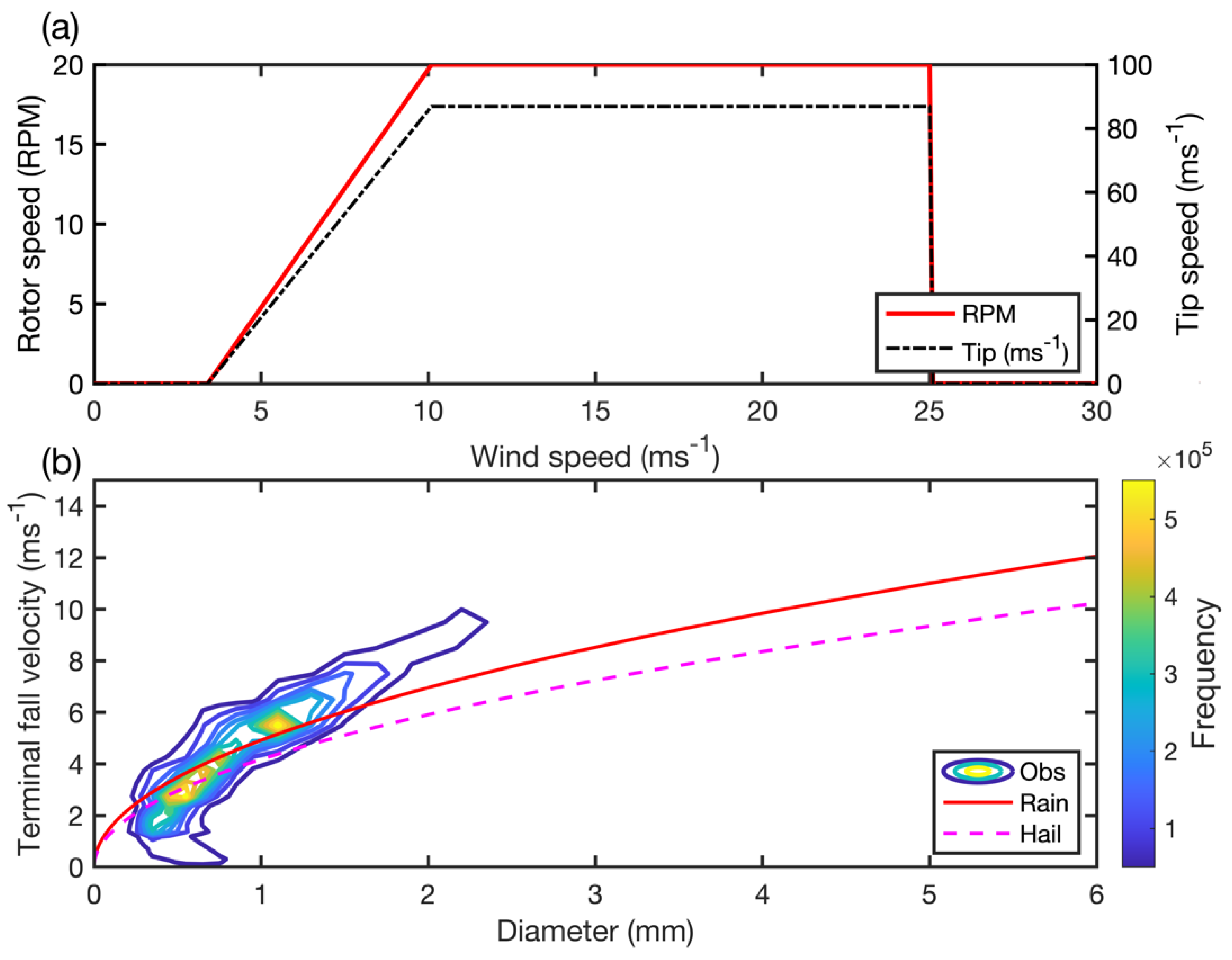
The closing velocity between the hydrometeors and the blade. Variations in wind turbine rotational speed are a function of incident wind speed (WS) at the hub-height (Figure 1a). The rotational speed of the wind turbine blades during typical operation exceeds the terminal fall velocity (v_t) of hydrometeors and hence generally dominates the closing velocity between falling hydrometeors and wind turbine blades.

A range of approximations have been proposed to describe the dependence of hydrometeor v_t on their diameter (D), phase, morphology and density [39]. Estimates shown in Figure 1b are computed using:

$$v_{t,rain}=\kappa {\left[\frac{{\rho }_o}{{\rho }_{air}}R\right]}^{1/2}$$

(1)

where R = droplet radius (m), κ = 220 m^1/2s⁻¹, ${\rho }_o$ = air density at sea level (kgm⁻³), ${\rho }_{air}$ = air density at the altitude above sea level (kgm⁻³) [40]. Early research [41] suggested that droplet v_t should be calculated within three different diameter ranges. The following is valid for droplet diameters (D) > 0.05 mm (5 × 10⁻⁵ m);

$$v_{t,rain}=B\left\{1-exp\left[-{\left(\frac{D}{a}\right)}^n\right]\right\}$$

(2)

where for D = 5 × 10⁻⁵ m to 3 × 10⁻⁴ m, B = 1.91 ms⁻¹, a₁ = 3.16 × 10⁻⁴ m and n = 1.754. For D > 3 × 10⁻⁴ m, the coefficients in Equation (2) are adjusted to B = 9.32 ms⁻¹, a₁ = 1.77 × 10⁻³ m and n = 1.147.

An approximation for the terminal fall velocity for hail is:

$$v_{t,hail}={\left[\frac{8}{3}\frac{\left|g\right|}{C_D}\frac{{\rho }_i}{{\rho }_{air}}{R}_h\right]}^{1/2}$$

(3)

where R_h = radius of the hailstone (m), ${\rho }_i$ = density of ice (kgm⁻³), ${\rho }_{air}$ = air density at the altitude at which the hail is falling (kgm⁻³) and $C_D$ = drag coefficient (0.55) [40]. Alternative, simpler forms have also been experimentally determined. E.g., for D_max < 2.05 cm:

$$v_{t,hail}=12.65D_{max}^{0.65}$$

(4a)

For D_max > 2.05 cm:

$$v_{t,hail}=15.69D_{max}^{0.35}$$

(4b)

where D_max = hailstone maximum diameter [42]. For hail D of 0.6 to 9 mm, the following has been suggested [43]:

$$v_{t,hail}=3.74D^{0.5}$$

(5)

Virtually all droplets with D > 0.5 mm have sufficient inertia to deviate from the streamlines and impact the blade with an impingement efficiency ~1 and have a velocity at impaction close to v_t [14,44,45,46].

During periods when wind turbines are operating close to their rated capacity (i.e., generating electricity of an amount equal to their nameplate) and so are rotating at their maximum speed (Figure 1a), the v_t of hydrometeors (Figure 1b) contributes ≤10% of the net closing velocity between the droplets and blade. A possible exception to this may occur if hydrometeors are caught up in downdrafts or downbursts from convective systems [47].

(ii)

The number, size and phase of hydrometeors that impact the blade leading edge. The incubation, transition and steady-state progression of damage on leading edge [48] differs as a function of precipitation climate. There is evidence that larger drops are of greater importance in dictating the incubation period and that smaller drops are critical in the transition and steady-state progression [49]. Further, the materials response to hail (ice) differs from that to collisions with rain (liquid) droplets [35]. The maximum von-Mises stress created by impact of a 10 mm diameter hailstone on a blade leading edge greatly exceeds that from a rain droplet of equivalent size and closing velocity due to differences in mass and hardness [35]. Recent laboratory-based research found that for hailstone with diameters of 15 and 20 mm as few as five impacts at a closing velocity of ≥ 110 ms⁻¹ were needed to cause damage to a glass fibre reinforced plastic composite coated with polyurethane [50].

Larger wind turbines with higher rated capacity and longer blades are now being deployed [51,52,53]. These wind turbines typically use lower rotational speeds, but the length of the blade means they typically have higher tip-speeds than smaller, and lower rated (or nameplate) capacity wind turbines, and thus they may experience higher rates of LEE. That coupled with increased deployments offshore [52] where maintenance costs are considerably higher [54,55,56], led to the International Energy Agency Wind Technology Collaboration Programme (IEA Wind TCP) to create Task 46. This task is designed to undertake cooperative research in the key topic of blade erosion. The goal is to improve understanding of the drivers of LEE, the geospatial and temporal variability in erosive events, erosion mechanics, the impact of LEE on wind plant performance and the cost/benefit of possible mitigation strategies.

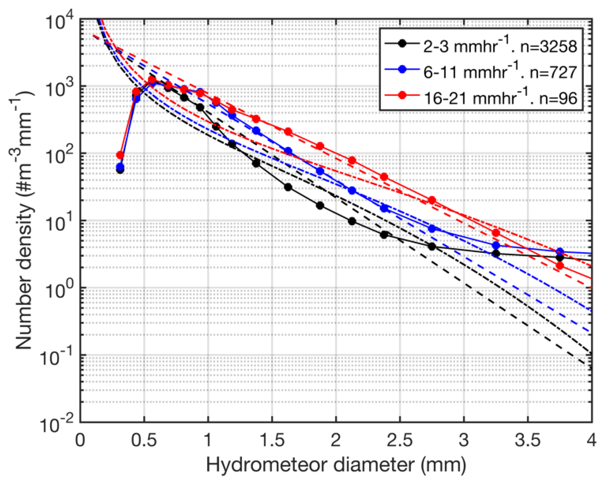
1.2. Hydrometeor Droplet Size Distributions

Although theoretical droplet size distributions (DSD) are often formulated in terms of the number of droplets above some threshold radius (or diameter), observed droplet size distributions measure hydrometeor counts in diameter classes and thus are processed to generate number concentrations (dN) within some finite size interval (dD). They are expressed as the number concentrations of raindrops per cubic meter as a function of their diameter normalized for a fixed size interval (dN/dD or N(D), #m⁻³ mm⁻¹).

It has long been recognized that increasing precipitation intensity (or rain rate, RR) shifts the hydrometeor DSD towards an increase in the relative abundance of larger droplets [57]. Accordingly, theoretical DSD are described as a function of prevailing RR and/or liquid water content (LWC) of air. Frequently, the number DSD for rain droplets is assumed to follow a two- or three-parameter gamma distribution [58], although there is some evidence to suggest a three-parameter lognormal may be optimal under some circumstances [59]. The normalized gamma distribution as a function of LWC (in gm⁻³) is given by:

$$N\left(D\right)=N_{w}f\left(\mu \right){\left(\frac{D}{D_m}\right)}^{\mu }exp\left[-\left(4+\mu \right)\frac{D}{D_m}\right]$$

(6)

where N_w is:

$$N_w=\frac{{3.67}^4{10}^{3}LWC}{\pi {\rho }_w{D}_0^4}$$

(7)

and D_m is:

$$D_m=\frac{4+\mu }{3.67+\mu }{D}_0$$

(8)

where D₀ = median drop diameter, ρ_w = density of water and μ = shape parameter of the distribution that can be derived by fitting to observed DSD [45]. Details on estimation of N_w and ƒ(μ) are given in Testud et al. [60].

The Marshall-Palmer approximation for DSD for rain was experimentally derived based on data collected in Montréal, Canada in 1946 [61]. It assumes that rain droplets follow an exponential distribution and can be easily used to predict the size distribution of liquid hydrometeors (rain droplets) based on the prevailing rainfall rate (RR, in mmhr⁻¹) [61]. It is most frequently expressed as the number of droplets above radius, R, per cubic meter of air (N, m⁻³):

$$N=\frac{N_0}{\Lambda }{e}^{-\Lambda R}$$

(9)

where $\Lambda =8200{\left(RR\right)}^{-0.21}$ (m⁻¹) and $N_0=1.6\times {10}^7{\mathsf{m}}^{-4}$.

The Det Norske Veritas (DNV) Recommended Practice for LEE testing issued in December 2020 and amended in October 2021 [46] proposes use of the so-called Best rain DSD to characterize the droplet size spectrum. This distributional form was published in 1950 and is based on measurements made in the United Kingdom using filter paper [41]. It has the form:

$$N\left(D\right)=\frac{W}{V}\left(\frac{k_B·D^{k_B-1}}{a^{k_B}}\right)e^{-\lfloor D/a{\rfloor }^{k_B}}$$

(10)

where V = spherical volume of the droplet $\left(\frac{1}{6}\pi D^3\right)$ (mm⁻³), D = droplet diameter (mm), W = total water volume which is given as 67 RR^0.846 (mm³) RR = rainfall rate in mmhr⁻¹, k_B = 2.25, a = 1.3 RR^0.232.

The DNV Recommended Practice also suggests 6 mm as an upper bound for droplet diameter asserting that above this diameter “aerodynamic forces break up the droplet” [46]. As shown herein, observations derived using ground-based disdrometers suggest the existence of droplets at diameters considerably above 6 mm.

Fewer studies have examined the size distribution of hail stones [62,63]. The simplest approximations use a single fitting parameter (λ), e.g.,:

$$N\left(D\right)=115{\lambda }^{3.63}{e}^{-\lambda D}$$

(11)

where D = hail stone diameter [64]. Values of λ of 0.3 to 0.6 mm⁻¹ were proposed based on measurements in Canada [64,65].

It should be noted that rain droplets are generally not spherical and are increasingly oblate as D increases. For liquid droplets the ratio of the vertical to horizontal axis decreases from about 1 for D = 1 mm, to 0.7 at D = 5 mm [66]. The following empirical estimate of the terminal fall velocity for deformed rain droplets has been advanced for 0.04 ≤ R ≤ 2.5 mm:

$$v_{t,rain}=-c_1\left[w_0-w_{1}exp\left(\frac{R_o-R}{R_1}\right)\right]$$

(12)

where R = equivalent droplet radius of the deformed drop of a sphere with the same volume (mm), w₀ = 12 ms⁻¹, w₁ = 1 ms⁻¹, R₀ = 2.5 mm, and R₁ = 1.0 mm. c₁ is a density correction factor given by the square root of the ratio of 70 kPa to the air pressure at the height of the droplet [40].

Smaller hail stones (i.e., D < 5 mm) are almost spherical, but for massive hail with D > 50 mm, the ratio of the vertical to horizontal axis can drop to 0.6 [67]. This may have some important implications when considering the area of impact on a wind turbine blade. Further, the material stresses induced by hail stone impacts will inevitably be dictated in part by the hardness or strength (tensile and compressive) of the solid hydrometeors, that is determined in part by their density. Although many hailstones have densities close to 900 kgm⁻³ some of the largest natural hailstones exhibit a lower density [67].

1.3. Spatial Variability in the Primary Drivers of Leading Edge Erosion

Previous meteorological research has indicated substantial spatial variability in the intensity, frequency and annual accumulation of liquid precipitation and frequency of hail at the global scale. High spatial variability in annual precipitation accumulation has been documented using homogenized records of in situ measurements such as the Global Historical Climatology Network (GCHN) dataset [68] (Figure 2a), blended multi-stream datasets (e.g., Global Precipitation Climatology Centre (GPCC) Full Data Reanalysis Version 7 [69]) Figure 2b), and satellite-derived estimates [70]. Annual precipitation accumulation varies by a factor of 10, even within individual countries (e.g., the US). Further, a recently released data set that merges information from multiple instruments and measurement technologies found that daily precipitation accumulation on the top 1 percent of wet days (i.e., days with daily accumulated precipitation of >1 mm) ranges from <5 mm over large parts of Australia, interior regions of Asia, northern Africa and western North America to >80 mm over large swaths of South America, parts of the eastern US, India and southern China [71].

Hail frequency also varies greatly across different parts of the globe [72]. An analysis of hail observations from the US National Oceanic and Atmospheric Administration (NOAA) Storm Prediction Center’s event database, and similar archives from Australia and Europe, found that when the data are conditionally sampled to include only events with maximum hail diameter >25 mm, the annual hail frequency per 100 by 100 km grid cell are over 20 times higher in large parts of the south-central US than either Europe or Australia [73]. Similar spatial patterns in hailstorm frequency are found based on analyses of multi-sensor multi-wavelength brightness temperature data from the GPM mission (Figure 2c). An additional assessment of hail occurrence from Microwave Humidity Sounders onboard a number of different satellites also identifies the Southern Great Plains (SGP, south-central portions of the continental US) as being a global hot-spot for hail occurrence particularly during the Northern Hemisphere (NH) warm months. Secondary maxima are identified in central Eurasia and South America during the NH cold months [74]. It should be noted that these hail climatologies are biased towards detecting large-scale convective events (i.e., those that have long-duration—i.e., last for multiple hours and large spatial scales) [75].

There are also important gradients in the frequency of precipitation and hail at the regional and sub-regional scale. For example, based on data from the Integrated Multi-satellitE Retrievals for the Global Precipitation Measurement (GPM) mission (IMERG) [76], the median size of precipitation systems over North America ranges from < 10,000 km² in parts of the west to 50,000 km² in the US southeast [77]. The mean intensity ranges from below 1 mmhr⁻¹ in the west to well over 2 mmhr⁻¹ in the US southeast [71]. On sub-regional scales there is also high variability. For example, annual precipitation varies by a factor of 10 across Texas and the prevalence of hail events ranges from hundreds of 5 min events per year to nearly zero [78]. Northwestern Texas has high wind turbine installed capacity and a high joint probability of hail and/or heavy precipitation at power-producing wind speeds [78].

Figure 2. (a) Map of mean annual precipitation (mm) computed from the Global Historical Climatology Network (GCHN) dataset (v4) for all 10,468 measurement sites with complete records for the five years; 2015–2019. Location (magenta dots) of the primary sites from which hydrometeor and wind data are presented herein. Listed west to east these sites are; Southern Great Plains, United States (US SGP), Canada coastal, UK coastal, Norway coastal, North Sea, and Denmark. (b) Map of mean annual precipitation (mm) from the GPCC Full Data Reanalysis Version 7 (data have a spatial resolution of 1 by 1 degree). (c) Map of estimated annual hail frequency at 2 deg resolution based on the NASA Passive Microwave Hail Climatology Data Products V1 data set and observations from 2014–2022 [75]. (d) Map showing countries that have either more than 5 GigaWatts (GW) of wind energy installed capacity (IC) onshore or more than 1.5 GW offshore (as of end of 2020) based on data from the GWEC 2020 status report [79].

Figure 2. (a) Map of mean annual precipitation (mm) computed from the Global Historical Climatology Network (GCHN) dataset (v4) for all 10,468 measurement sites with complete records for the five years; 2015–2019. Location (magenta dots) of the primary sites from which hydrometeor and wind data are presented herein. Listed west to east these sites are; Southern Great Plains, United States (US SGP), Canada coastal, UK coastal, Norway coastal, North Sea, and Denmark. (b) Map of mean annual precipitation (mm) from the GPCC Full Data Reanalysis Version 7 (data have a spatial resolution of 1 by 1 degree). (c) Map of estimated annual hail frequency at 2 deg resolution based on the NASA Passive Microwave Hail Climatology Data Products V1 data set and observations from 2014–2022 [75]. (d) Map showing countries that have either more than 5 GigaWatts (GW) of wind energy installed capacity (IC) onshore or more than 1.5 GW offshore (as of end of 2020) based on data from the GWEC 2020 status report [79].

Wind speeds and wind resources also vary across a wide range of spatial and temporal scales [80,81,82]. This leads to an uneven distribution of wind turbine deployments (Figure 2d), and to large spatial variability in the amount of time wind turbines operate at their maximum rotor rotational speed (Figure 1a).

Precipitation frequency and intensity (RR) are highly dependent on the spatial and temporal resolution of observations. Generally, intensity-duration-frequency curves to illustrate the approximately exponential decline in RR with increasing temporal (and spatial) averaging [83,84]. Use of 1 h integration periods profoundly truncates the right tail of the probability distribution of RR relative to higher frequency observations [85]. For this reason, most data sets presented herein sample RR and DSD at a 1 min averaging period.

Relatively few long-term measurements of hydrometeor DSD are available. However, past research has postulated that regions dominated by stratiform precipitation generally have smaller median and mass-weighted mean droplet diameters. Conversely, those that exhibit a higher frequency of convective precipitation, especially where the convection is sufficiently vigorous to pass the freezing level and thus for there to be substantial ice in the cloud are a larger contribution from bigger droplets. According to some estimates, convective events have median droplet diameters for that are >3 times as large as those from stratiform events with the same droplet distribution intercept parameter (N_w), which is linked to the cloud LWC (see Equations (6)–(8)) [58,79].

1.4. Objectives

From the discussion above it is reasonable to postulate that spatiotemporal variations of hydroclimate conditions and the joint probabilities of WS and RR, DSD and hydrometeor phase will lead to variations in the accumulated kinetic energy into wind turbine blades, the resulting materials stress and hence the likelihood of erosion of the leading edge. It is further reasonable to postulate that the cost effectiveness of the different LEE preventative measures will vary in space.

Research reported herein is conducted under IEA Task 46 WorkPackage 2 Climatic conditions driving blade erosion and focusses on evaluating and analyzing observational data sets pertaining to the primary atmospheric drivers of wind turbine blade leading edge erosion; hydrometeors. Our objectives are as follows:

(1)

Review and summarize metrologies for measuring RR and DSD. Because of our focus is on wind turbine blade LEE, we concentrate on performance at high rainfall rates, for larger diameter hydrometeors and for detection of solid hydrometeors (hail and graupel).

(2)

Summarize aspects of hydroclimates (e.g., RR, hail frequency) at study locations with high wind energy penetration and/or high wind energy potential.

(3)

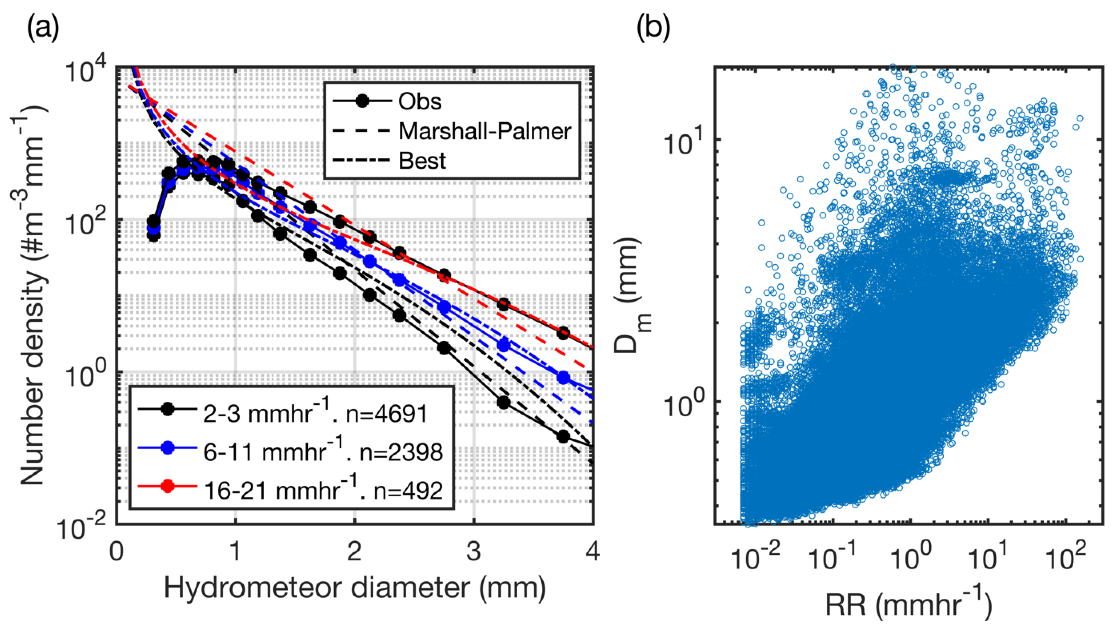
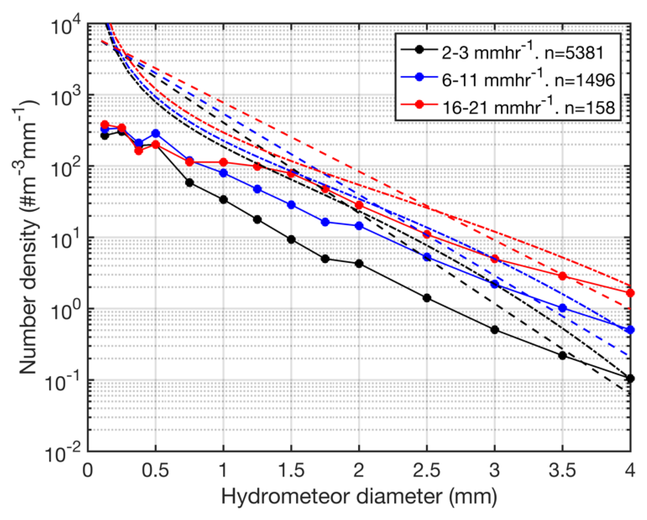
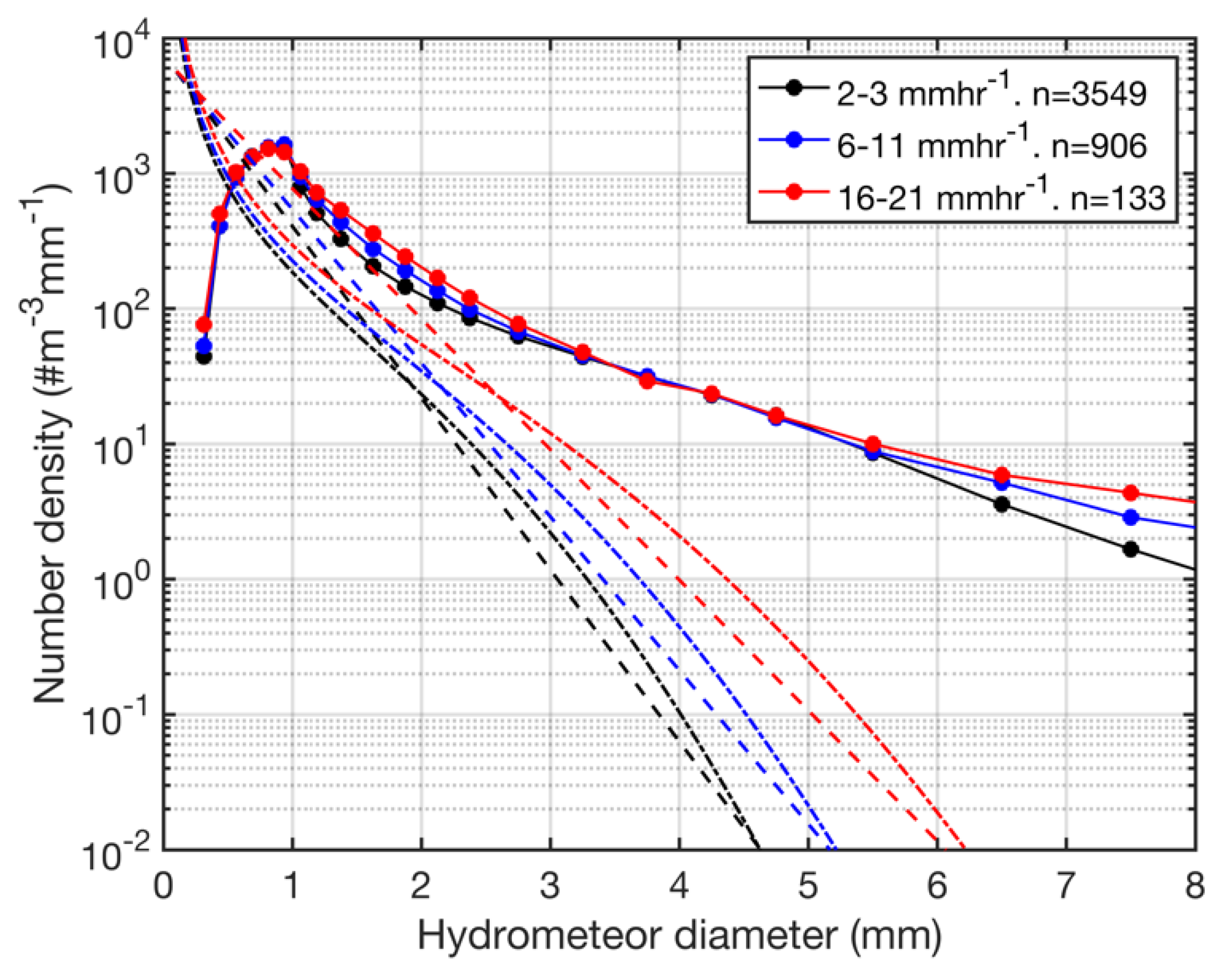
Compare observed DSD at several sites, and evaluate the degree to which the Marshall-Palmer and/or Best distributions accurately represent the observations. We further assess whether current whirling-arm experimental designs that use the Best DSD to guide the droplet sizes used are optimal to fully characterize surface impact resistance at different RR.

(4)

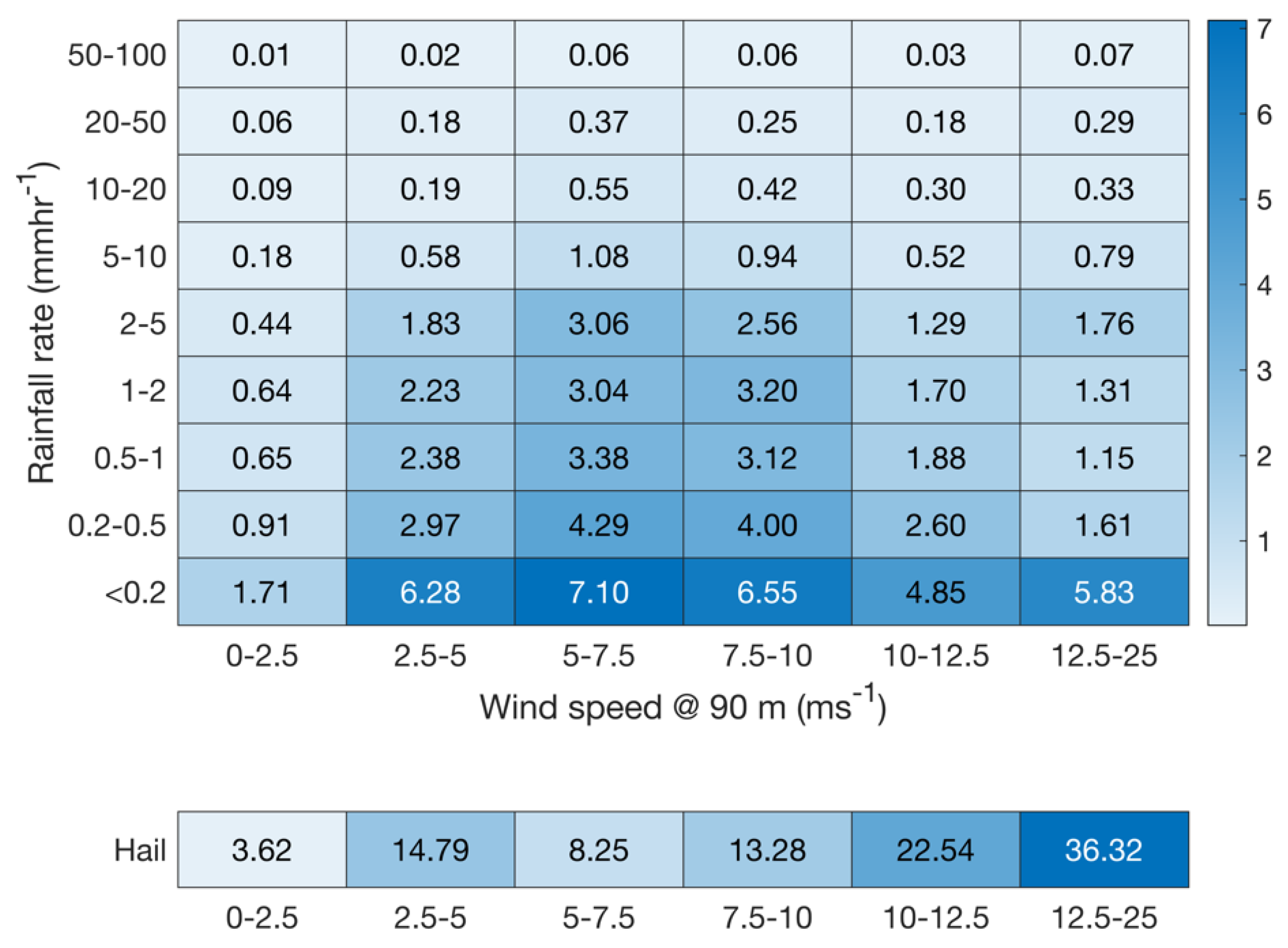
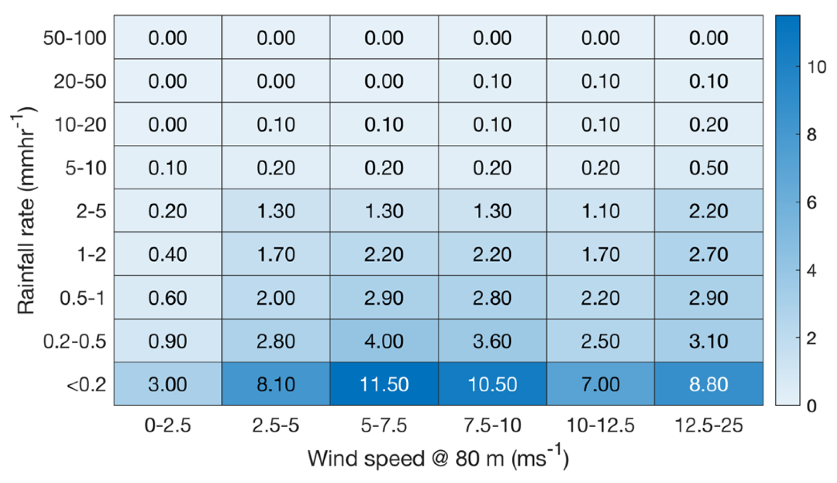
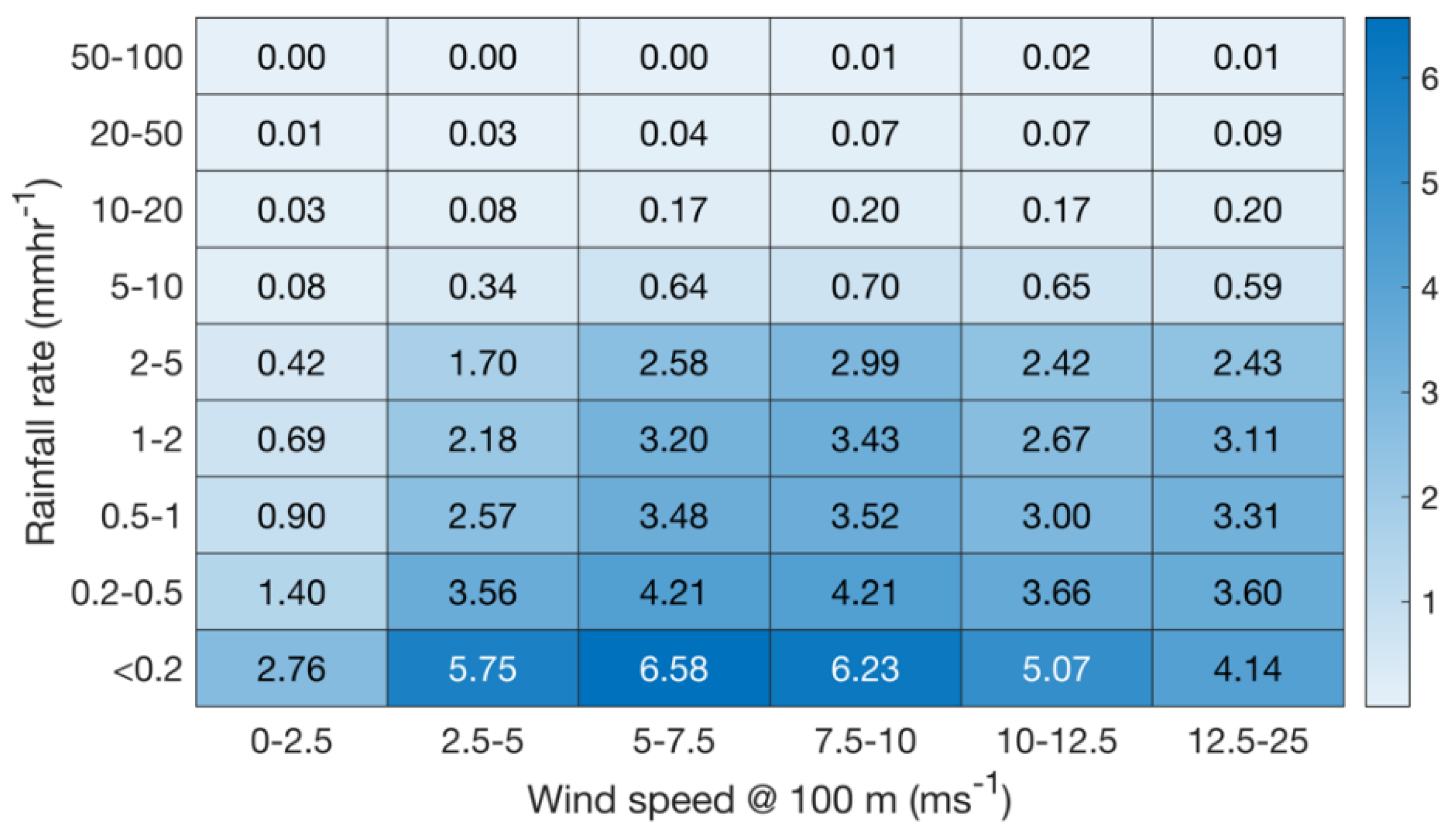
Summarize and compare joint probability distributions of wind speed and rainfall rates (and hail occurrence) to illustrate how inferences can be drawn regarding likely relative LEE potential.

We further articulate research activities required to provide high-fidelity assessments of key atmospheric drivers of LEE and to make a priori estimates of likely LEE severity at a given location and through time.

2. Materials and Methods

2.1. Metrologies for Measuring Rainfall Rates and Droplet Size Distributions

Most national meteorological measurement networks use heated tipping-bucket or weighing rain gauges to measure liquid-equivalent precipitation accumulation over a time interval (i.e., the RR). These data are often reported with a resolution of one hour [86], although some countries report data for selected sites at higher temporal resolution [87]. Some meteorological services equip these rain gauges with wind shields to reduce precipitation under-catch (particularly of snow) under high wind conditions [88].

Rain gauges remain the primary source of ground-truth information regarding precipitation receipt at the ground. Good agreement for daily accumulated precipitation (within ±10%) is generally reported from closure experiments [86]. These measurements, plus RR and hydrometeor phase estimated from ground-based dual polarization Doppler RADAR [89,90], are extremely important to hydrological applications [91]. They have relevance to, but are not sufficient for, estimation of kinetic energy transfer to wind turbine blades. This specific application requires high temporal resolution in order to capture high intensity but short duration precipitation events, plus information regarding the DSD. Thus, in past analyses, estimates of RR and hail occurrence from tipping bucket or weighing rain gauges and/or derived from ground-based dual polarization Doppler RADAR have been combined with approximations of DSD as a function of RR (Equations (6)–(11)) and simultaneous WS observations to derive estimations of time varying and annual accumulated kinetic energy transfer to wind turbine blades [78,92]. However, such estimates are critically dependent on the degree to which the assumed rain and hail DSD represent real atmospheric conditions.

Precipitation DSD can be measured using a range of different metrologies [93]. Two-dimensional video disdrometers (VDIS) comprises two video cameras with perpendicular lines of sight [94,95]. Objects passing through the measurement area obstruct the light and are detected as shadows by the cameras [96,97]. Impact disdrometers work by recording the kinetic energy transferred due to the impact of a falling hydrometeor on a detector [98,99]. Acoustic disdrometers work by detecting the acoustic signal generated by rain droplet impacts on a diaphragm [93]. Herein we present data primarily from optical disdrometers (also known as light occlusion instruments) that measure droplet number and fall velocity in a number of diameter classes by detecting the breaking of a horizontal light sheet by the passage of the hydrometeors [95,100,101]. As with rain gauges, the quality of data obtained from disdrometers can be influenced by wind-induced under-sampling of hydrometeors [102,103] and reporting of unrealistically low v_t for large D in high wind speeds [104]. In situ disdrometers are also subject to interference from other droplets (e.g., sea spray or splash) in the sample volume [103,105]. Thus, all disdrometers should be shielded using similar technologies to those deployed for rain gauges.

The process of translating the signal from a disdrometer to number density normalized by the diameter range covered in a given class is shown in Equation (13) and described below using the example of the 2nd generation OTT Particle size and velocity (Parsivel²) optical disdrometer [95,106]:

$$N\left(D_i\right)=\frac{n_i}{Ft{v}_t\left(D_i\right)∆D_i}$$

(13)

where n_i = number count in diameter class i (D_i in mm), F = area field of view of the disdrometer (0.0054 m² for the OTT Parsivel² disdrometer), t = sampling interval (typically 60 s), v_t(D_i) = fall velocity of a drop of that diameter (ms⁻¹), ΔD_i = width of the size class (mm). N(D_i) thus has units of the number per cubic meter of air per mm. Because of the low signal-to-noise ratio, the first two diameter classes for the Parsivel² (D_i of 0.062 and 0.187 mm) are frequently empty, thus valid data are generally reported for diameter classes with D_i of 0.25 mm and above. Note: The different generations (first and second) of the OTT optical disdrometer are denoted here as Parsivel¹ and Parsivel², respectively.

Previous research has indicated errors in the OTT Parsivel² terminal fall velocities under some atmospheric conditions [106] which may have some implications for the number density estimates reported herein (see Equation (13)). A key aspect of the data analysis framework for optical disdrometer observations pertains to use of screening procedures to exclude droplets reported in the raw measurements as occurring in terminal fall velocities that differ substantially from theoretical estimates of v_t(D_i). An illustration of this effect is given in Figure 3 for ~14,000 1 min observed hydrometeor counts expressed in diameter and fall velocity classes from measurements with an OTT Parsivel² deployed on the campus of Cornell University in upstate New York, US. As shown in Figure 3, while the mean number counts in combined D and v_t class illustrate the expected monotonic increase of fall velocity with droplet diameter, a non-trivial number of detected hydrometeors exhibit fall velocities below 2 ms⁻¹ even for D > 2 mm. These values may reflect the presence of insects and leaves in the instrument field of view, or splintered hydrometeors that strike on the housing of the disdrometer and subsequently enter the field of view. The implication is that it may be appropriate to remove them prior to computing the hydrometeor DSD. For example, in processing of data from optical disdrometers operating at US Department of Energy sites, droplets reported in fall velocity classes that differ by >±50% from the terminal velocity for water droplets in stagnant air computed using Gunn and Kinzer [107] are assumed to be in error and are excluded from consideration [101]. This inevitably results in a reduction in N(D_i). Currently there is no consensus regarding use of this screening to exclude some count data and/or the specific threshold that should be applied. We recommend best-practice be developed to ensure comparability of observed DSD across different sites and regions.

Some droplets pass through the margins of the field of view of the disdrometer. Thus, a further key aspect of the processing of disdrometer data pertains to use of an effective sampling area (F_eff) that scales with the droplet diameter. The following estimate of F_eff has been proposed [108]:

$$F_{eff}=L\left(W_A-\frac{D_i}{2}\right)$$

(14)

where L and W_A are the length (180 mm) and width (30 mm) of the viewing area.

Assuming spherical droplets, the precipitation rate (RR in mmhr⁻¹) is:

$$RR=\frac{\pi }{6}\frac{3.6}{{10}^3}\frac{1}{Ft}\sum n_i{D}_i^3$$

(15)

The mass-weighted mean diameter (D_m in mm) is computed as the ratio of the 3rd to the 4th moment of the measured droplet size distribution as follows [109]:

$$D_m=\frac{M_4}{M_3}$$

(16)

where:

$$M_n={\displaystyle \sum }_{i=1}^{NB}N\left(D_i\right)D_i^n∆D_i$$

(17)

where NB = number of size bins available from the disdrometer.

The Thies Laser Precipitation Monitor (LPM) optical disdrometer [110] works on a similar measurement principle to the OTT Parsivel and also measures hydrometeors as they fall through, and thus break, a series of adjacent horizontal beams. The Thies LPM disdrometer uses a wavelength (λ_w) of 785 nm, while the OTT Parsivel² operates at a λ_w = 650 nm. The Thies LPM used at sites in the UK Disdrometer Verification Network (DiVeN) experiment [111] employs 20 diameter classes from ≥0.125 mm to >8 mm and 20 velocity classes from 0 ms⁻¹ to 10 ms⁻¹. For the OTT Parsivel² disdrometer the 32 measured size classes range from mid-point diameters of 0.0619 to 24 mm and the 32 velocity classes range from 0.2 to 20 ms⁻¹. The OTT Parsivel² manual denotes an expected accuracy of ±10% in RR but does not provide information regarding the expected accuracy of the DSD. Previous work has reported highest relative uncertainty for low RR, larger diameter hydrometeors and short integration times [112]. For example, a study reported a sampling uncertainty in number concentrations of 5–11% for D of 1–2 mm, and for a D of 1.5 mm, an uncertainty of 8% for 1 min samples to 4.5% for a 10-min sampling period [103].

The presence of solid hydrometeors (snow, graupel, hail) is represented in data output from the OTT Parsivel² using the World Meteorological Organization (WMO) synoptic present weather codes (WC). WC of 71–73, inclusive indicate snow. WC of 87 (RR < 1 mmhr⁻¹, soft hail), 88 (RR ≥ 1 mmhr⁻¹, soft hail), 89 (RR < 2.5 mmhr⁻¹, hail) and 90 (RR ≥ 2.5 mmhr⁻¹, hail). The hydrometeor type classification is based on a combination of the v_t, and D following a look-up chart approach [100,113]. All optical disdrometers exhibit some uncertainty due to incorrect v_t assigned to hydrometeors that fall through the edge of the sampling area [112] and/or strong winds causing misclassification of hydrometeor type.

Present Weather Sensors (PWS) such as the Campbell Scientific PWS100 [39] use two or three optical sensors and measure the scintillation as individual hydrometeors pass through the illuminated volume. Hydrometeor type is determined by the relative contributions of light reflection, refraction and diffraction [39]. The PWS100 has been withdrawn from service, but measured droplet sizes range from 0.1 to 30 mm in 34 diameter classes and 34 velocity classes [114].

Ground-based remote sensing devices are also available that can also be used to infer RR and the size distribution of hydrometeors. Micro-rain RADAR (MRR) are active vertically pointing remote sensing systems. The Doppler shift of the backscattered radiation scales with the fall velocity of hydrometeors, which in turn is a function of their size. For MRR an assumption is made that the fall velocity of a droplet is equal to the terminal fall velocity which thus assumes the droplets are embedded in still air which is a source of uncertainty in deeply convective environments. The strength of the signal (backscatter intensity) scales with the number and size of hydrometers. Hence, the DSD can be computed and used to obtain an inferred RR. MRR provide the vertical profile (to heights of several kilometers) of hydrometeor properties including DSD at high temporal sampling rates (every 10 s) [115,116,117]. New techniques are being actively pursued to derive robust assessment of precipitation type based on the hydrometeor fall velocity, equivalent RADAR reflectivity, and diameter plus the presence (or not) of a bright band [118]. A key challenge in use of such technology is linking properties above the surface (even in cloud) to those at the ground, and modification of the hydrometeors as they fall through the atmosphere.

An additional area of active instrument development pertains to detection and sizing of hail. Hail pads are simple and cheap and hence have been used in community-based networks (e.g., Community Collaborative Rain, Hail and Snow network (CoCoRaHS) [119]). However, they provide time-integrated measurements and are labor intensive. The hail DSD are inferred from subjective assessment of dents caused by the hail impacts (e.g., in Styrofoam blocks wrapped in heavy duty aluminum foil) [120], some of which may overlap leading to undercounting of hail stones [121]. Next generation sensors (e.g., HailFlow sensor HF4 from ISAW) use acoustic technology. A key issue in all of these metrologies is the small sampling area which may systematically under-count large diameter hail [120]. Proposals for use of drone aerial photogrammetry for hail sampling have also been advanced [122].

As indicated by the brief precis given above, the metrologies for measuring hydrometeor DSD and even RR differ in terms of the size range to which they exhibit sensitivity and assumptions regarding the hydrometeor morphology. For example, the OTT Parsivel² disdrometer uses a calibration procedure to derive a relationship between the droplet diameter in the vertical and horizontal axes and applies an assumed (but unspecified) function to relate each sample of oblate spheroid droplets to a RR [100]. It has been reported that the assumed axis ratio relationship in the OTT Parsivel² varies linearly with diameter for D = 1 to 5 mm from 1 to 0.7 and is set to 0.7 for D > 5 mm [66].

2.2. Statistical Methods

Analyses of the frequency and intensity of precipitation (RR) and the frequency of occurrence of hail across the six primary sampling locations presented herein are summarized using the following statistical approaches. The probability of hail is computed as the ratio of the frequency with which the hail flag is reported by the sensor divided by the total number of observational periods for which data are available. The probability of precipitation (PoP) is described using two different RR thresholds for precipitation detection; 0 mmhr⁻¹ and 0.2 mmhr⁻¹. The latter threshold is used to enable comparisons across instruments that may have different minimum detectable limits for precipitation. To characterize the upper percentiles of the probability distribution of RR, we also report the 90th, 95th and 99th percentile RR (mmhr⁻¹) during all periods with non-zero RR. These values thus provide information regarding RR when the heaviest precipitation is occurring. To illustrate the importance of high-frequency sampling of precipitation in the context of wind turbine blade LEE, data from the optical disdrometer at the US SGP site [95] (Figure 2a and Figure 4a) are subject to an analysis wherein each hour of data where any precipitation occurred are sampled to compute the maximum RR with sampling durations of 1-, 5-, 10-, 20-, 30- and 60-min. The results are then summarized to compute the 10th, 20th, … 90th percentile values of the resulting RR for each averaging period.

Non-parametric Spearman (rank) correlation coefficients (r_s) are reported as a measure of the degree of agreement between two data sets. This measure of correlation is appropriate for use with data, such as RR, that are not Gaussian distributed [123]. Linear fitting is undertaken and is expressed in terms of the slope (m) and the intercept (c) of the general linear model, where x is the independent variable and y is the dependent variable:

$$y=mx+c$$

(18)

To illustrate RR and DSD from different instrument metrologies we examine data from three disdrometers deployed at the US SGP site (Figure 4a). The degree of closure between RR is assessed using three different thresholds (RR > 0.1, 1 and 10 mmhr⁻¹) using contingency-table based metrics; the Hit Rate (HR) and the False Alarm Rate (FAR) [123]. The HR, which is also known as the proportion correct, is the ratio of the number of times data from the two instruments agree on precipitation occurrence for each of the thresholds, to the total number of times that the reference instrument (in this case the OTT Parsivel²) exhibited a RR in excess of that threshold. The FAR, is a measure of the number of times both instruments indicated RR below the specified threshold, to the number of times the reference instrument indicated RR below the specified threshold. Thus, perfect agreement would result in HR = 1 and FAR of 0.

Wind speed data from both the ERA5 reanalysis [124] and NORA3 hindcast [125] for a height of 100 m AGL [124] plus observationally derived wind speeds at each site at/close to typical wind turbine hub-heights are presented. They are summarized in part by fitting them to a two-parameter Weibull distribution using maximum likelihood methods and reporting the scale and shape distribution parameters (A and k) [123,126]:

$$f\left(WS\right)=\frac{k}{A}{\left(\frac{WS}{k}\right)}^{k-1}exp\left[-{\left(\frac{WS}{A}\right)}^k\right]$$

(19)

In the joint probability analysis of WS and RR we discretize the WS into six classes reflecting different operating ranges of a typical wind turbine (Figure 1a). Class 1 with WS of 0–2.5 ms⁻¹ reflect periods with no rotor rotation. WS class 2: 2.5–5 ms⁻¹ indicate periods with only very slow rotation. WS classes 3 (5–7.5 ms⁻¹) and 4 (7.5–10 ms⁻¹) indicate periods when the rotational speed is likely to be increasing and the last two classes (5 and 6), WS: 10–12.5 and 12.5–25 ms⁻¹ indicate periods when, depending on the precise wind turbine in operation, the RPM will be close to and at the maximum speed, respectively.

2.3. Locations from Which Data Are Presented

Analyses presented herein focus primarily on data from six locations (Figure 2a and Figure 4a,b) that are listed by longitude (west to east) and summarized below (Table 1).

Table 1. Summary of the locations from which data are reported herein.

Location Label Used Here	Site	Latitude	Longitude	Instrument Type Used for Droplet Size Distribution Measurements	Instrument Used for the Wind Speed Measurements (Height)	Weibull Distribution Parameters	Sampling Period from Which Data Are Reported
US SGP	DoE ARM, Lamont, SGP, USA	36.6072° N	97.4875° W	OTT Parsivel2	Doppler lidar (90 m AGL)	A = 8.96 ms−1 k = 2.183	January 2017–December 2020
				2D Video
				Impact
US NE	Cornell University, New York, USA	42.4534° N	76.4735° W	OTT Parsivel2	None	N/A	December 2021, July–September 2022
Canada coastal	WEICan, Canada	47.035° N	64.015° W	CSI PWCS100	Cup anemometer (80 m AGL)	A = 10.3 ms−1 k = 2.001	October 2018–December 2020
Coastal UK	WAO, UK	52.9433° N	1.1414° E	Thies LPM	None	N/A	February 2017–September 2019
Norway coastal	Bergen, Norway	60.38° N	5.33° E	OTT Parsivel2	ERA5 reanalysis [124] NORA hindcast [125] 2D sonic anemometer (49 m ASL)	A = 6.7 ms−1 k = 1.7 A = 7.0 ms−1 k = 1.7 A = 4.0 ms−1 k = 2.0	January 2016–December 2021
				MRR			January 2010–December 2014 and January 2016–December 2021
North Sea	Horns Rev, Denmark	55.6° N	7.59° E	OTT Parsivel2	None	N/A	December 2018–October 2021
Denmark inland	DTU, Denmark	55.693° N	12.1° E	OTT Parsivel2	Cup anemometer (94 m AGL)	A = 8.0 ms−1 k = 2.4	June 2019–December 2021

Table 1. Summary of the locations from which data are reported herein.

Location Label Used Here	Site	Latitude	Longitude	Instrument Type Used for Droplet Size Distribution Measurements	Instrument Used for the Wind Speed Measurements (Height)	Weibull Distribution Parameters	Sampling Period from Which Data Are Reported
US SGP	DoE ARM, Lamont, SGP, USA	36.6072° N	97.4875° W	OTT Parsivel2	Doppler lidar (90 m AGL)	A = 8.96 ms−1 k = 2.183	January 2017–December 2020
				2D Video
				Impact
US NE	Cornell University, New York, USA	42.4534° N	76.4735° W	OTT Parsivel2	None	N/A	December 2021, July–September 2022
Canada coastal	WEICan, Canada	47.035° N	64.015° W	CSI PWCS100	Cup anemometer (80 m AGL)	A = 10.3 ms−1 k = 2.001	October 2018–December 2020
Coastal UK	WAO, UK	52.9433° N	1.1414° E	Thies LPM	None	N/A	February 2017–September 2019
Norway coastal	Bergen, Norway	60.38° N	5.33° E	OTT Parsivel2	ERA5 reanalysis [124] NORA hindcast [125] 2D sonic anemometer (49 m ASL)	A = 6.7 ms−1 k = 1.7 A = 7.0 ms−1 k = 1.7 A = 4.0 ms−1 k = 2.0	January 2016–December 2021
				MRR			January 2010–December 2014 and January 2016–December 2021
North Sea	Horns Rev, Denmark	55.6° N	7.59° E	OTT Parsivel2	None	N/A	December 2018–October 2021
Denmark inland	DTU, Denmark	55.693° N	12.1° E	OTT Parsivel2	Cup anemometer (94 m AGL)	A = 8.0 ms−1 k = 2.4	June 2019–December 2021

These sites are selected due to the availability of detailed hydroclimatic observations and their location in regions with large wind resource and/or wind energy deployments:

(1)

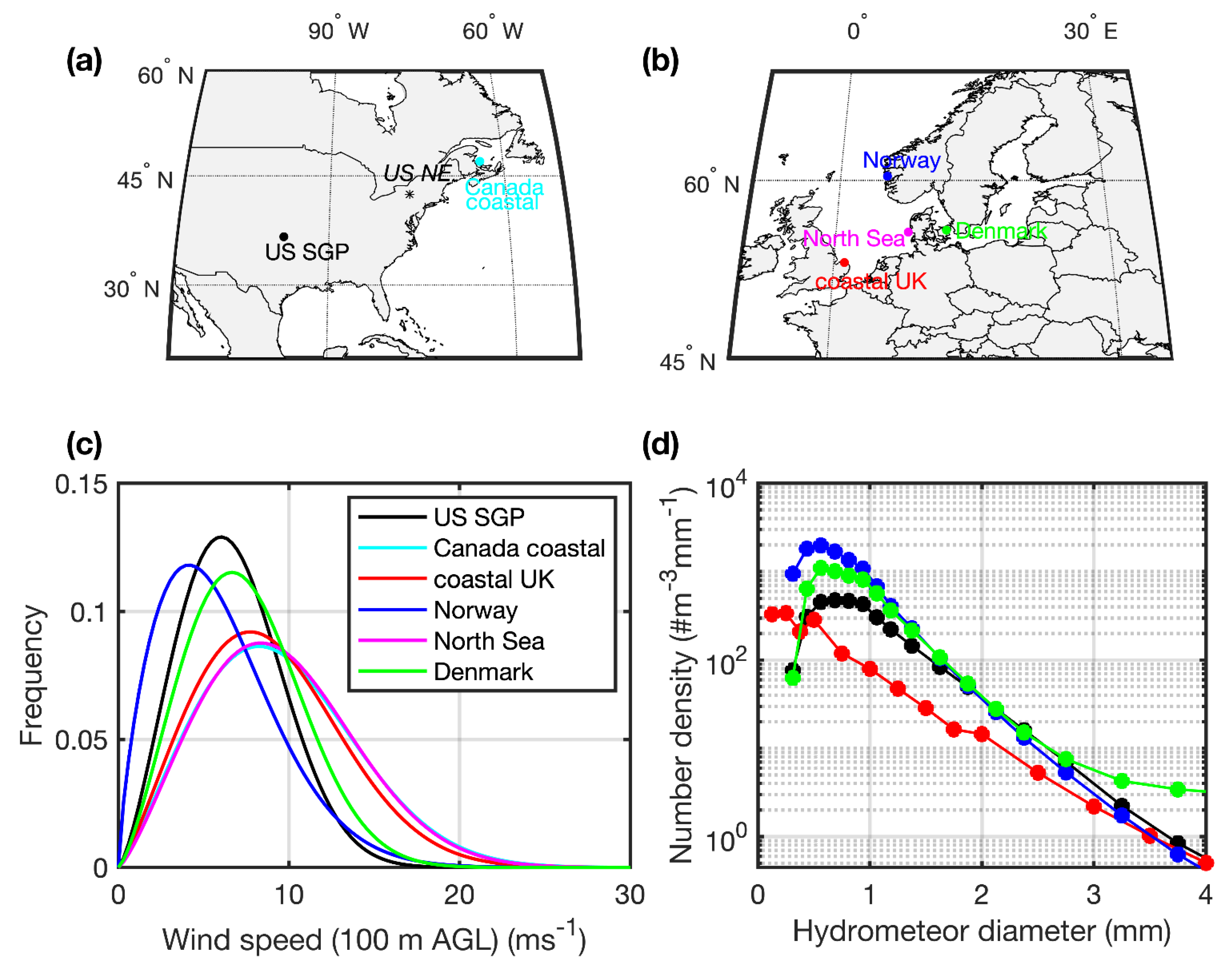
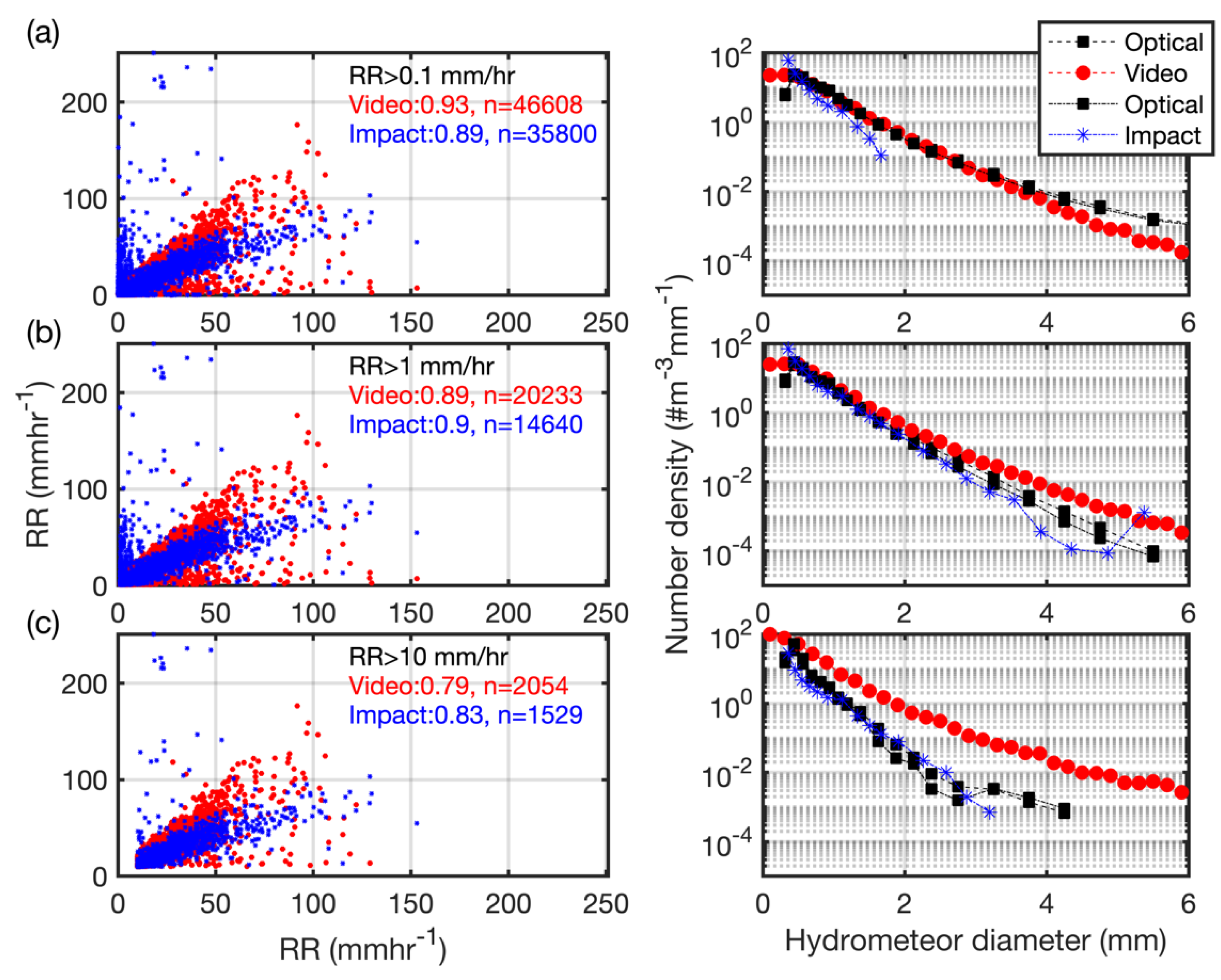
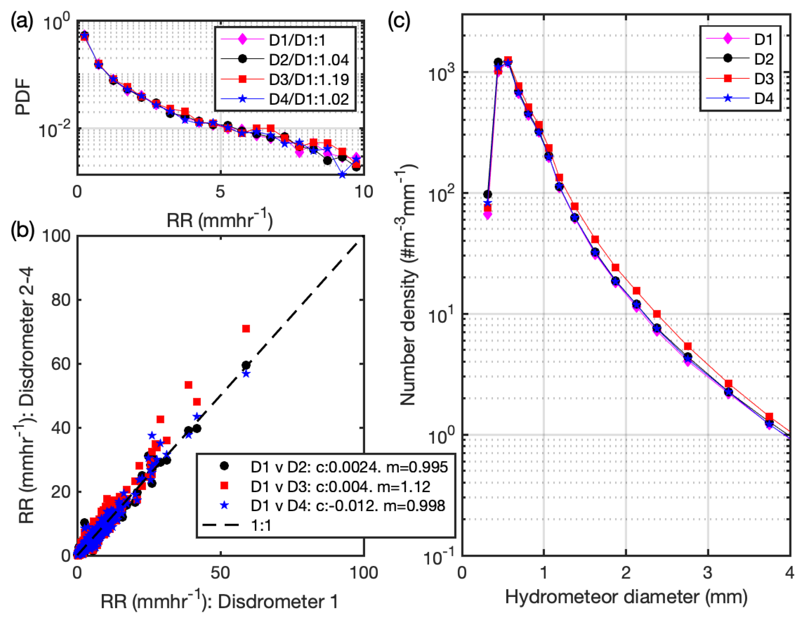
Southern Great Plains, United States (US SGP): The US Department of Energy (DoE) Atmospheric Radiation Measurement (ARM) site at Lamont in Oklahoma. DSD data from three disdrometers deployed at this site are reported; an impact disdrometer [99], an optical (Parsivel²) disdrometer [101] and a video disdrometer [95]. Data availability during 1 January 2017 to 31 December 2020 from the OTT Parsivel² is 93%. All disdrometers are recorded every 1-min. To provide a context for the spatial variability in DSD and RR derived from a range of locations, we compare measurements of RR and DSD from these three different disdrometers. It is important to recall that they have different sampling ranges. The Parsivel² discretizes the hydrometeors into 32 diameter classes, with classes centered at diameters of 0.062 to 24 mm. The video disdrometer uses 50 diameter classes from 0.1 to 9.9 mm. The impact disdrometer uses 20 diameter classes from 0.359 to 5.373 mm. Wind speed data reported for this site are 15 min average values and derive from a Halo Photonics Doppler lidar [127]. As described further below, the US SGP region is subject to frequent deep convection and associated high RR and hail [92,128,129]. There are also substantial wind turbine deployments. Based on data from the USGS wind turbine database (updated from [130]), as of April 2022, there are over 16 GW of wind turbine installed capacity (IC) within 300 km of the US SGP site considered here. This is over 12% of the total US wind turbine IC.

(2)

Canada coastal: The Wind Energy Institute of Canada (WEICan) on Prince Edward Island in eastern Canada. The site has 300 degrees of ocean exposure and contains five 2 MW DeWind turbines that have a hub-height of 80 m AGL, as well as an instrumented 80 m meteorological tower compliant with IEC 61400-12-1 and a 10 m meteorological tower compliant with IEC 61724-1 [131]. Hydroclimatic data presented herein derive from a Campbell Scientific PWS100 deployed at 11 m AGL and the RR data availability is 88.9%. Due to a data logging issue no DSD are available. Wind speed observations are from a Thies cup anemometer at 80 m AGL which is the hub-height of the wind turbines operating at WEICan.

(3)

UK coastal: The Weybourne Atmospheric Observatory (WAO) [132], on the north coast of the English county of Norfolk. WAO was one of 14 sites at which Thies LPMs ran as part of the Disdrometer Verification Network (DiVeN) project [111]. This site has an altitude of 16 m above sea level and is landward of a pebble beach. It has an open ocean fetch to the north and a clear view towards many of the major offshore wind farms operating in the western North Sea around the coast of East Anglia. The closest offshore wind farms are; Sheringham Shoals, a 317 MW installation 17–23 km north of the north Norfolk coast, and Race Bank, a 573 MW installation approximately 27 km north-northwest of Weybourne. No in situ or remote sensing wind speeds are presented from this location due to a lack of availability of well-documented, traceable measurements at/close to wind turbine hub-height.

(4)

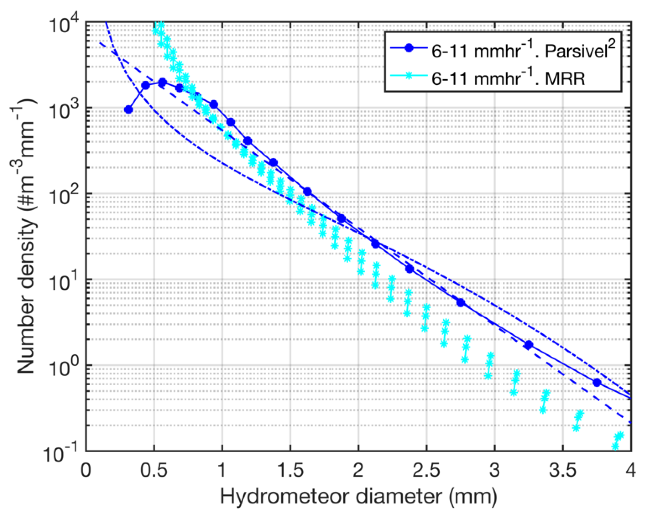
Norway coastal: The Geophysical Institute at the University of Bergen on the west coast of Norway. The RR and DSD presented here are from a METEK MRR [117,133] operated on a building rooftop (39 m above sea-level (ASL)), and an OTT Parsivel². Wind speeds are observed using a 2D sonic anemometer on a co-located 10 m mast (49 m ASL). The offshore waters along the west coast of Norway have large wind resources. When commissioned the 94.6 MW Hywind Tampen floating offshore wind farm (140 km from the Norwegian coast and northwest of Bergen) will be the largest floating wind farm in the world [134].

(5)

North Sea: Horns Rev2 offshore wind farm off the west coast of Denmark in the North Sea. RR and DSD data are from an OTT Parsivel² deployed at a height of 22 m ASL. The Horns Rev offshore wind farm comprises three wind turbine clusters; Horns Rev 1 (160 MW), Horns Rev 2 (209 MW) and Horns Rev 3 (407 MW) located approximately 30 km from the Danish west coast. No wind speed measurements are presented from this location since they are deemed commercially sensitive.

(6)

Denmark: The Risoe campus of the Danish Technical University (DTU) near Roskilde in Denmark. Denmark was an early adopter of wind technologies and has nearly 6000 wind turbines deployed onshore [135] and nearly 2 GW of offshore installed capacity [79]. The RR and DSD reported herein derive from OTT Parsivel² instruments recorded with 1 min and 10 min averaging.

Uncertainty in the wind speed during precipitation events has a substantial impact on the implied closing velocity between the rotating blade and the falling hydrometeors and thus the kinetic energy transferred by hydrometeor impacts. This is because of the highly non-linear dependence of the turbine rotational speed and hence tip speed on the incident wind speed (Figure 1a). Hence, except at the site in Norway, the joint probability analyses are based on observations rather than once hourly output from gridded reanalysis or hindcast products.

Additional data are presented for an instrument closure experiment performed on the campus of Cornell University in upstate New York (US NE, Table 1). We present data from two campaigns. The first lasted from 21 October 2021 to 7 December 2021 and the second was performed during 14 July 2022 to 30 September 2022 (Table 1). Both involved co-deployment of four OTT Parsivel² disdrometers and capture of over 6000 1 min periods of precipitation.

3. Results

3.1. Hydroclimate and Wind Regimes at the Focus Sites

Wind speeds at a height of 100 m AGL from the ERA5 reanalysis [124] at the six focus study locations (Table 1) are summarized in Figure 4c. Consistent with observational WS data, all six locations exhibit probability distributions that are consistent with substantial wind resources. The fidelity of ERA5 wind speeds varies in space and there is lowest fidelity in regions of complex terrain [136]. This is also evident in comparisons of the Weibull parameters in ERA5 relative to the measurements from coastal Canada (WEICan) and the US SGP. At the US SGP location, the measurements at 90 m AGL indicate a Weibull A and k of 8.96 ms⁻¹ and 2.183, while the ERA5 output for 100 m AGL indicates values of 7.55 ms⁻¹ and 2.391, which suggests a negative bias in the wind speeds at this location and a narrowing of the probability distribution. The negative bias at the US SGP site is consistent with past research that has indicated negative bias in ERA5 wind speeds over western North America [136]. At WEICan (coastal Canada), the Weibull A and k derived from observations at 80 m are; 10.3 ms⁻¹ and 2.001, respectively, while those from ERA5 for 100 m AGL are 10.7 ms⁻¹ and 2.239, also indicating a substantially narrower probability distribution from ERA5. For this reason, the joint probability distributions presented herein use only local wind speed observations. It should be noted that much closer agreement is found for the onshore site in Denmark consistent with the surrounding flat terrain. ERA5 wind speeds at 100 m AGL have a Weibull A of 8.40 ms⁻¹ and k = 2.368 while similar values computed from the observations from the cup anemometer at 94 m AGL are; 8.0 ms⁻¹ and 2.4.

As expected based on the site descriptions in Section 2.3, coastal Norway exhibits the highest frequency of precipitation and is the location with highest annual mean precipitation (2250 mm). The US SGP exhibits a high frequency of hail and the highest values for the 90th, 95th and 99th percentile RR (

Table 2. Summary of precipitation statistics at the six primary long-term study sites for all available instruments. PoP denotes probability of precipitation and is computed using two different rainfall rate (RR) thresholds. * The values for the three disdrometers at US SGP reflect all 1 min periods when all three instruments reported valid data. Probability of hail/graupel is defined using hail as Weather Codes (WC) 87, 88, 89, 90, except for Bergen where the OTT Parsivel² indicates a very high prevalence of WC 87 or WC 88 (2.8% of all observations have one of these two codes). Unless otherwise stated the sampling intervals over which the data are averaged is 1-min. See DSD for these sites in Figure 5, Figure 6, Figure 7, Figure 8 and Figure 9.

Location Label Used Here	Site	Instrument Type	Sampling Period	Probability of Hail/Graupel * (%)	PoP (RR > 0 mmhr−1) (%)	PoP (RR > 0.2 mmhr−1) (%)	90th, 95th, 99th Percentile Values of RR (mmhr−1)
US SGP	DoE ARM, Lamont, SGP, USA *	OTT Parsivel2	January 2017–December 2020	0.059	4.20	2.81	4.18, 7.72, 31.3
		2D Video		N/A	6.28	2.40	2.45, 4.70, 20.1
		Impact		N/A	6.53	1.76	1.79, 3.68, 15.5
Canada coastal	WEICan, Canada	CSI PWCS100	October 2018–December 2020	None reported	7.47	3.81	1.99, 3.18, 9.52
Coastal UK	WAO, UK	Thies LPM	February 2017–September 2019	0.0094	12.3	5.17	1.69, 2.97, 9.44
Norway coastal	Bergen, Norway	OTT Parsivel2	January 2016–December 2021	0.08	20.5	14.3	2.43, 3.98, 10.1
		MRR (100 m AGL)	January 2010–December 2014 and January 2016–December 2021	N/A	18.6	10.4	1.98, 3.48, 9.37
		MRR (200 m AGL)		N/A	18.2	12.9	3.23, 5.60, 19.4
		MRR (300 m AGL)		N/A	18.1	13.4	3.76, 6.56, 19.4
North Sea	Horns Rev, Denmark	OTT Parsivel2	December 2018–October 2021	N/A	6.9	4.1	1.68, 2.73, 7.75
Denmark inland	DTU, Denmark	OTT Parsivel2	June 2019–December 2021	0.03	7.4	4.19	2.05, 3.27, 8.59
		OTT Parsivel2 (10 min)		0	11.6	4.72	1.82, 2.85, 7.15

). Based on the four years of data from the Parsivel² disdrometer non-zero precipitation is reported during about 4.2% of all 1 min records and the 90th, 95th and 99th percentile 1 min RR are; 4.18, 7.72 and 31.3 mmhr⁻¹, respectively. Thus, 1% of minutes when precipitation is falling (or 220 min in an average year) exhibit a RR > 31.3 mmhr⁻¹. Precipitation is more frequently observed at coastal Canada, coastal UK, coastal Norway, North Sea, and Denmark, but each of those sites has a much lower frequency of hail reports. Further all have considerably lower 99th percentile RR of 9–10 mmhr⁻¹ (coastal Canada, coastal Norway, and coastal UK) and ≈7–8 mmhr⁻¹ (North Sea and Denmark) (Table 2). These analyses illustrate that the US SGP exhibits a hydroclimate that differs substantially relative to sites in Europe with respect to parameters of importance to wind turbine blade LEE. Indeed, hail may dominate LEE in the US SGP [92], in contrast to northern Europe where the hydroclimate is dominated by liquid precipitation, hail is very infrequent (Table 2) and thus kinetic energy transfer to the blades is likely dominated by rain [137,138]. This would seem to imply that exclusion of consideration of hail in whirling-arm experiments may lead to inaccurate assessments of blade coating lifetimes for wind turbines deployed in regions such as the US SGP and in other regions with high hail frequency such as southern Europe, Asia, Africa and Australia (Figure 2).

The DSDs from the Parsivel² disdrometer at the US SGP site sampled for different RR emphasize a long-recognized feature of precipitation: That, although there is a high degree of event-to-event variability (Figure 5) [139], on average higher RR are associated with increases in droplet number plus increases in the median droplet diameter (D₀) and mass-weighted mean diameter (D_m) due to the presence of more larger droplets [57]. This finding is equally applicable to measured DSD from the five other sites (Figure 6, Figure 7, Figure 8 and Figure 9).

Neither the Best nor Marshall-Palmer approximations of the DSD fully represent the shape of the observed DSD from the disdrometers deployed at US SGP, or Norway, or coastal UK or Denmark (Figure 5, Figure 6, Figure 7 and Figure 9). The Marshall-Palmer approximation yields DSD that are in closer accord with the observations but tends to overestimate the number of smaller droplets and underestimates the number of larger droplets. The underestimation is evident for D > 2.5 mm for all three RR at the US SGP site, for D > 1.25 mm in Denmark and D > 0.7 mm at coastal Norway. Data from the Thies LPM operated WAO (coastal UK) exhibit DSD that are lower than either Best and Marshall Palmer approximations up to droplet D of 1.5 mm. However, larger droplet (D > 3 mm) number concentrations are overestimated by the Best approximation and underestimated by Marshall-Palmer (Figure 6). These results indicate that assessment of accumulated kinetic energy transfer to wind turbine blades and the resulting materials stress, and blade lifetimes that use measured RR combined with assumed DSD are likely to result in inaccurate assessments that may be mis-leading to windfarm developers. We recommend that where possible such any such assessments be predicated on either on-site or near-by DSD measurements.

Despite the large degree of site-to-site variability for mean DSD at a given RR (Figure 4d) and the variability at a given site in different RR classes (e.g., Figure 5a), the slope of all DSD curves (number density as a function of droplet diameter) from all sites exhibit a shallower gradient with D than are manifest in either the Best or Marshall-Palmer approximations especially at high RR. This is particularly important given the relevance of high RR and the associated larger droplet diameters to potential kinetic energy to the rotating blades.

The implication of these analyses is that if whirling-arm experiments are sampling DSD from Best rain droplet distribution they are not fully representing atmosphere-relevant DSD. Such experiments may be under-sampling the abundance of larger droplets (D > 0.5 mm) that are likely to induce the largest material stresses [140]. For this reason, we recommend that RR and DSD considered in whirling-arm experiments be greatly expanded to cover a wider range of conditions. It is also noted that the highly accelerated RET do not realistically represent operational modes for wind turbines and have the drawback that for viscoelastic coatings other damage types may be observed. Thus, use of lower speeds to better reflect real-life wind turbine blades in service may be advantageous. Furthermore, we recommend use of a broad-spectrum of droplet sizes (similar to the spray mode used in Bech et al. [140]) rather than a nearly uniform D currently used for the testing, and that the suggestion to confine the range of droplet D to < 6 mm as recommended in the DNV Recommended Practice be reconsidered.

Data from the North Sea offshore wind farm indicate a DSD that deviates substantially from the other locations from which data are presented and also from theoretical expectations (Figure 8). DSD from this disdrometer may reflect the presence of a mixed droplet distributions due to both hydrometeors and sea spray. Sea spray droplets range in diameters from <1 μm (film droplets, generated by biogeochemistry and bubble bursting), to 1–50 μm (jet droplets, generated by bubble bursting and the impact of rain droplets on the sea surface), to spume droplets that have diameters up to a few mm and are generated by wave tearing and wave breaking on structures/vessels [141,142]. Such mixed DSD have been previously demonstrated in data collected using a disdrometer at 16 m ASL on an offshore marine tower in Japan [105]. In light of this issue, we do not consider the North Sea data set further. Nevertheless, production of high-quality hydrometeor size distributions and precipitation intensity datasets from disdrometers or other sensors installed on offshore platforms (e.g., buoys and/or meteorological masts, transformer platforms) is essential to quantifying LEE potential for offshore wind turbines. We recommend that either; (i) hydrometeor DSD measurements at offshore wind farms for the purpose of LEE analyses be performed preferentially using remote sensing devices (e.g., MRR). By virtue of sampling higher above the surface, they may be less vulnerable to sea spray contamination. Or alternatively, (ii) studies be conducted to investigate and quantify the influence of sea spray on such measurements and develop filtering methods for data quality control based on wind speed, wave properties, etc.

When the mean DSD from optical disdrometers at four of the sampling sites are compared for the same fixed RR interval, the results indicate important differences (Figure 4d). Some of these differences may derive from the relatively small sample size at some locations and/or differences in measurement technology (at coastal UK). It is noteworthy that the DSD reported above for our selected study sites are in contrast to a year of data collected using a PWS100 disdrometer deployed 5.5 km off the east coast of the UK [143]. Analyses of those data indicated “the Best DSD significantly overestimates the diameter of droplets” [143]. The reason for this discrepancy is currently unresolved, but it may also to linked to the different disdrometer technology used. The influence of different measurement strategies and instrument metrologies are discussed further below. Additional causes of differences in DSD are likely geophysical and include different abundance of cloud condensation nuclei in marine and continent locations, the presence or absence of solid hydrometeors and a difference in the relative frequency of convective versus stratiform precipitation. These differences strongly indicate the need for development of disdrometer networks in regions with high wind resource potential in order to develop a tool for use in a priori estimation of LEE potential.

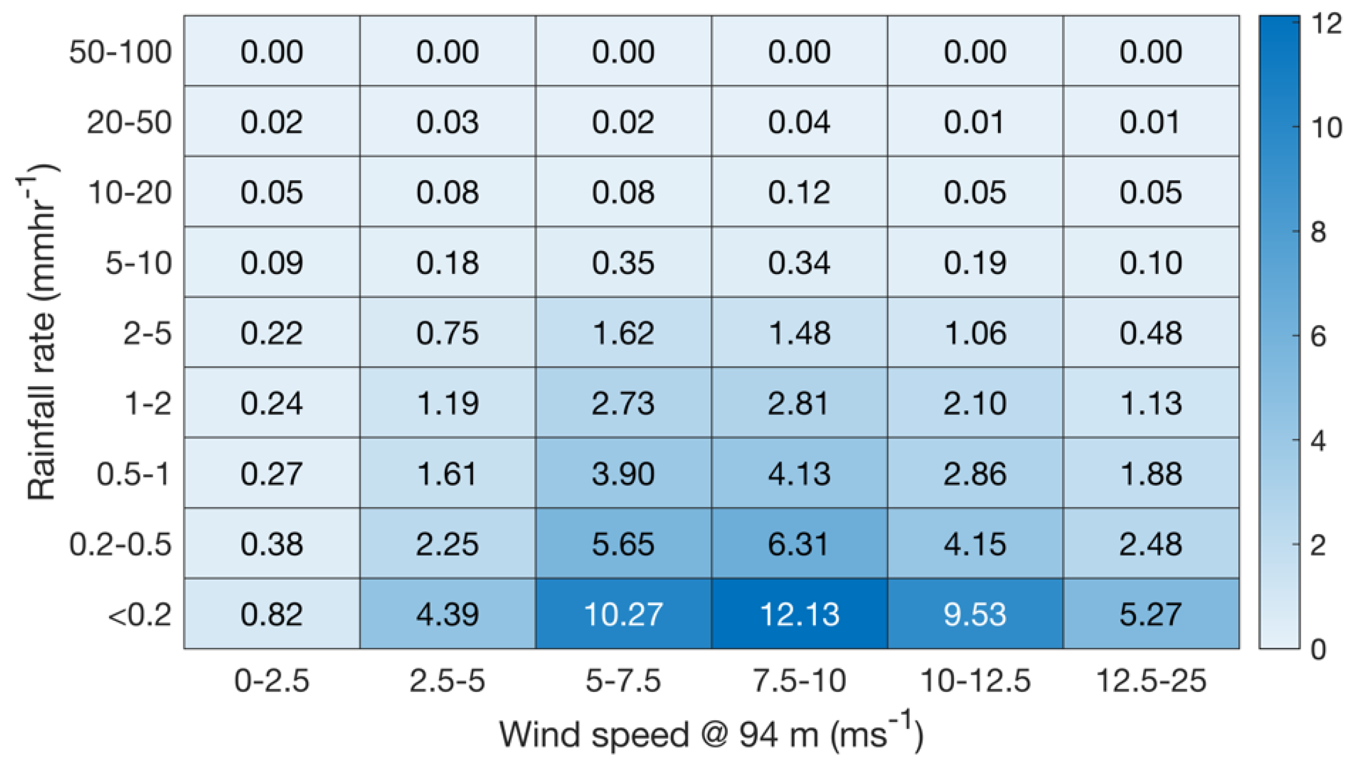
3.2. Joint Probabilities of Hydroclimatic Conditions and Wind Speeds

Based on the discussion in Section 1, it is clear that the closing velocity between hydrometeors and wind turbine blade and the kinetic energy transfer to the blades are maximized under the joint occurrence of high RR with a large fraction of high diameter droplets (Figure 5) and/or hail and high wind speeds when the blades are likely to be rotating at their maximum speed. Accordingly, any blade lifetime estimate is going to be critically contingent on the joint distributions of RR (and DSD and phase) and WS. Examples of the joint distributions of RR and hub-height wind speed are given in Figure 10, Figure 11, Figure 12 and Figure 13 for four illustrative sites; the US SGP, coastal Canada, coastal Norway and the onshore site in Denmark. In construction of these illustrative joint-probabilities, wind speeds are assumed to be constant over each 1 min period within each t-minute periods over which the wind speed data are collected.

Laboratory studies and numerical models have repeatedly shown that impact responses on the wind turbine blade coating system increase with “increasing droplet size and increasing droplet impact angle with maximum impulses, stresses and damages developed for normal impingement (90°)” [15]. A numerical modeling study found that the number of impacts required for onset of erosion damage increases by a factor over seven when impact velocities are decreased from 140 ms⁻¹ to 80 ms⁻¹ under RR > 25 mmhr⁻¹ [15]. Hence, in much of the following discussion we focus on the relative frequency of joint occurrence of high RR and high wind speeds.

At the US SGP site >2.4% of 1 min precipitation events, or 0.1% of all 1 min periods, are associated with wind speeds at which typical wind turbines will be rotating at their maximum speed (or close there-to) (WS = 10–25 ms⁻¹) and RR > 5 mmhr⁻¹ (Figure 10). Conversely at the coastal Canada site (WEICan) only 1.2% of 1 min precipitation events, which is 0.09% of all 1 min periods, are associated with these conditions (Figure 11). At the site in Bergen (noting the WS are from the NORA3 hindcast), 2.3% of all 1 min periods with precipitation and 0.47% of all 1 min periods in an average year are associated with WS between 10 and 25 ms⁻¹ and RR > 5 mmhr⁻¹ (Figure 12). At the site in Denmark 0.46% of all 1 min periods with precipitation and 0.04% of all 1 min periods in an average year are associated with WS between 10 and 25 ms⁻¹ and RR > 5 mmhr⁻¹ (Figure 13).

Focusing on the even more extreme portion of the joint distributions; RR > 10 mmhr⁻¹ and WS of 12.5–25 ms⁻¹, these occur on average on ~200 min per year at the US SGP site, on ~60 min in an average year at coastal Canada and 30 min in Denmark. Thus, all other things being equal material stresses in blades on wind turbines operating in the US SGP will be higher than at these other two locations. The implied enhanced material stress at the US SGP site is amplified by the high frequency of co-occurrence of WS of 12.5–25 ms⁻¹ and hail (~100 min in an average year).

Naturally, the interannual variability and seasonal variability in the frequency of hail and/or heavy RR means the joint probability heatmaps shown in Figure 10, Figure 11, Figure 12 and Figure 13 must be viewed and compared with caution. They are constructed using relatively short data time series and in order to increase the sample size have not been screened to ensure they have equal representation of each season (Table 1). However, they represent the types of analyses that are necessary as a first step in the development of robust climatologies for use in assessing wind turbine blade lifetimes. The low frequency of highly erosive events that are likely to dominate kinetic energy transfer to the blades and resulting materials stresses also emphasizes the critical need for long-duration data sets to properly characterize LEE potential. It is therefore recommended that reference sites such as that operated at the US SGP DoE ARM be deployed at additional locations and run for many years in order to generate robust and comparable data sets.

In closing it is important to re-emphasize that uncertainty in disdrometer-based RR is enhanced under high wind speeds [144]. This is of particular concern to efforts to derive estimates of the kinetic energy transfer to wind turbine blades and also merit further investigation.

3.3. Influence of Measurement Strategies and Instrument Metrologies

As described above, precipitation events exhibit a wide range of durations and fluctuating RR during individual events. This is illustrated using data from OTT Parsivel² instruments operating in the US SGP and in Denmark. Ten percent of all 60 min periods when precipitation occurred at US SGP exhibit a 1 min maximum RR > 4.5 mmhr⁻¹ (Figure 14). When the time series are averaged to 30 min sampled periods the 90th percentile RR (i.e., that exceeded by 10% of the data) is 2.1 mmhr⁻¹. Given the non-linear dependence of the DSD on RR (see Equations (6)–(10) and Figure 5, Figure 6, Figure 7, Figure 8 and Figure 9), use of 30 min or 60 min average RR will greatly under-sample the presence of large droplets and thus kinetic energy transfer into the blades. Data from two OTT Parsivel² instruments operated at the Denmark site with different integration periods also illustrates the expected dependence of RR on the averaging period. Based on 1 min sampling, the 99th percentile RR is 8.6 mmhr⁻¹. When sampled at 10 min the 99th percentile RR is 7.2 mmhr⁻¹. For accurate estimation of kinetic energy transfer to wind turbine blades it is thus recommended to use very high frequency (ideally 1-min) sampling of DSD and RR.

Data from the OTT Parsivel² disdrometer at the US SGP also emphasizes important differences in DSD as a function of hydrometeor phase. The mean DSD when the data are conditionally sampled to select all 1133 periods when the WC indicates the presence of hail and/or graupel (mean RR ~14 mmhr⁻¹), and that from an equal number of periods with similar RR but only liquid hydrometeors. The results show clear evidence of a considerably higher frequency of large (D > 3 mm) droplets when hail is indicated (Figure 15). While this comparison is contingent on correct assignment of the WC by the disdrometer software, it reemphasizes the importance of research to better characterize DSD for hail and also that, even neglecting the influence from hydrometeor hardness, hail events are therefore likely be associated with higher kinetic energy transfer into the blade and potentially greater induced material stresses. Thus, we recommend enhancing efforts to include hail into material fatigue experiments. The hail DSD shown in Figure 15 also emphasizes the need for such experiments to include hailstones with diameters below 15 mm that was the lower limit considered in the study of Reshab [50]. Given the challenges in use of frozen water in such analyses particularly for smaller D [50], it may be preferable to use polylactic acid pellets to replicate the effects of hail impacts on wind turbine blades, since they have approximately the right hardness and tend to shatter on impact [130].

The regional differences in hydroclimates and the joint probability distributions of wind speeds and RR implied by the data summaries described in Section 3.1 have important implications for the spatial variability of WT blade LEE. However, it is important to note that they are also subject to differences associated with instrument metrology. Efforts to quantify this effect in the hydroclimatic parameters based on new data analyses are described below and presented in the context of the existing literature.

A number of previous studies have evaluated the relative accuracy of different disdrometers. Most have focused on comparisons of different optically based instruments (see summary given in

Table 3. Summary of some previous closure experiments for different disdrometers, and new findings from the current analysis.

Reference	Instruments Considered	Comparison of Accumulated Precipitation (acc. PPT) or Rainfall Rates (RR)	Comparison of DSD
Johannsen et al. [145]	PWS100, Theis LPM, Parsivel1	All underestimated of acc. PPT v weighing rain gauge	PWS100 higher modal D than Parsivel1
Guyot et al. [147]	Theis, Parsivel1		Theis LPM higher conc. of D < 0.6 mm
Tokay et al. [148]	Impact, 2DVD, Parsivel1	Negative bias in acc PPT in Parsivel1	Differences in DSD and total number concentration (2DVD and Parsivel1) amplified at high RR
Angulo-Martinez et al. [149]	Theis LPM and Parsivel2		Theis LPM lower median D than Parsivel2
De Moraes Frasson et al. [146]	Theis LPM and tipping bucket rain gauges	Large differences (18%) in seasonal acc PPT from 5 different Theis LPM disdrometers. Theis LPM positive bias relative to rain gauges.
Fehlmann et al. [43]	Theis LPM, 2DVD	Theis LPM negative bias in RR
Krajweski et al. [151]	2DVD, Parsivel1	RR consistently higher from Parsivel1	Parsivel1 higher droplet counts, 2DVD higher conc. of D > 4 mm
Chang et al. [30]	2DVD, MRR		MRR higher conc for D < 1 mm than ground-based disdrometers
Marzuki et al. [152]	Parsivel1, MRR	Lower RR from MRR	MRR higher conc for D < 1 mm, Parsivel1 higher conc for D > 2 mm
Sarkar et al. [150]	Theis LPM, MRR	RR MAE = 3 mm/hr between instruments, MRR RR lower than Theis LPM	Good agreement for D = 1–3 mm
Current study: US SGP	2DVD, Parsivel2, impact	RR higher from Parsivel2 by 10% v. 2DVD and 37% v. impact (0.1 mm/hr to define wet minute). Difference decreases with use of 1 mm/hr to define a wet minute, but increase for a threshold of 10 mm/hr	Impact disdrometer lower conc of D > 1 mm than Parsivel2
Current study: coastal Norway	MRR, Parsivel2		MRR higher conc than Parsivel2 for D < 1 mm

and following discussion). For example, one study at a site in Austria compared data from two PWS100, a Thies LPM and an OTT Parsivel¹ against a weighing rain gauge. All of the disdrometers underestimated accumulated precipitation by 2 to 29% relative to the rain gauge [145]. Mean droplet size spectra from Thies LPM showed lower number density for D > 1 mm. The PWS100 sensors had highest modal droplet D but exhibited important differences from each other. PWS100 showed 31 and 22% of droplets were in the diameter range 1–2 mm. Equivalent data from the Thies LPM and OTT Parsivel¹ indicated 6% and 16% [145]. Conversely a long-term study of multiple Theis LPM relative to tipping-bucket rain gauges found the Theis LPM tended to overestimated long-term accumulated precipitation, and that the Theis LPM exhibited differences in long-term accumulated precipitation of up to 18% [146]. A further study of the Thies LPM and an OTT Parsivel¹ conducted over 3 years in southern Australia found only small discrepancies between the two Thies LPM sensors, but greater differences between the two OTT Parsivel¹ instruments. The authors report “LPM recorded 1 to 2 orders of magnitude more smaller droplets for drop diameters below 0.6 mm compared to the OTT Parsivel¹, with differences increasing at higher rainfall rates” [147]. Analyses of accumulated precipitation and DSD from impact, 2DVD and OTT Parsivel¹ disdrometers indicated “reasonable agreement” in terms of total event accumulated precipitation with a reference rain gauge, with mean biases of −3.5%, +0.4% and −7.5%, respectively [148]. Relative to the impact and 2DVD, the OTT Parsivel¹ was negatively biased in terms of the number concentrations for D < 0.76 mm, and exhibited a positive bias for D > 2.44 mm. The divergence between the instruments was most marked for RR > 2.5 mmhr⁻¹ [148]. A further study lasting 2 years and employing two Thies LPM and two OTT Parsivel² disdrometers during >200 rain events, also found the Thies sensors exhibited a higher total number of droplets but considerably lower median droplet diameter, even after correcting for the differences in measured diameter range. The discrepancies were amplified at high RR [149]. An evaluation of the Thies LPM in terms of precipitation detection, intensity and phase relative to an OTT weighing precipitation gauge and a 2DVD found the HR for precipitation detection is 99% (FAR = 9.9%) during periods with liquid precipitation [43]. However, the Thies disdrometer underestimated rainfall intensities by 16.5% which the authors linked to under-sampling of the number concentration of hydrometeors with D of 0.5 to 3.5 mm relative to the 2DVD [43]. The slope of a linear fit of RR averaged to 30 min from the Thies disdrometer and the OTT pluviometer was equal to 0.80. The authors proposed adjusting the number concentrations of rain droplets in the first three diameter classes (D: 0.125–0.5 mm) down by factors of 0.83 to 0.92, and those in classes 4 to 12 (D: 0.5–3.5 mm) up by factors of 1.08 to 1.43, and those in classes 13 to 22 (D: 3.5 to > 8 mm) down by factors of 0.92 for class 13 to 0.19 for the 22nd (and largest) class [43]. A further study comparing optical and 2DVD disdrometers with an MRR found best consistency between number concentrations for D = 1.1 to 3.8 mm and for longer averaging periods [102]. That study also reported much higher number concentrations (higher by a factor of 10) for D < 0.5 mm from the MRR relative to the ground-based disdrometers. An additional study comparing MRR with the Theis LPM found persistently higher RR for the Theis LPM, and a lower concentration of droplets with D < 2 mm in the Theis LPM [150]. This feature of a negative bias in the concentration of smaller droplets measured by the ground-based disdrometer relative to the MRR is also seen in the Norway data presented here (Figure 7).

Comparison of 1 min RR and mean DSD conditionally sampled for three RR based on four years of data from the OTT Parsivel² disdrometer, video disdrometer and an impact disdrometer operating at the US SGP site further illustrate the key importance of metrology in dictating the implied hydroclimate and, by association, LEE potential (Figure 16, Table 2 and Table 3). The probability of precipitation computed using a RR threshold of 0 mmhr⁻¹ for all periods when all three disdrometers were operating show good closure between the 2D video disdrometers and the impact disdrometer, and both show a higher precipitation frequency than the OTT Parsivel² (Table 2). This finding may be partly attributable to differences in the diameter range to which the disdrometers are sensitive. Specifically, as mentioned above, the smallest size channel (centered at a D~0.062 mm) from the OTT Parsivel² has zero reports of droplets and the second channel centered at D~0.187 mm has very few reported droplets. Thus, the OTT Parsivel² has a functional observational range beginning at D~0.22 mm which is above the smallest diameter reported by the video disdrometer, though not the impact disdrometer.

When a RR threshold of 0.2 mmhr⁻¹ is applied, the probability of precipitation from the OTT Parsivel² exceeds that from the other two sensors. Over three-quarters of all 1 min periods when the optical, impact and video disdrometers were operating without error flags and the optical disdrometer indicated a RR above 0.1 mmhr⁻¹ are also identified as having RR > 0.1 mmhr⁻¹ (and RR > 1 mmhr⁻¹) in the video disdrometer (Table 3). It is notable that this HR is lower than that reported from an earlier study in Switzerland [43], but the FAR is also lower. This may reflect use of a screen to deselect periods with very light RR in the current analysis. For a RR threshold of 10 mmhr⁻¹, which equates to approximately the 96th percentile of all non-zero RR, and the 99.85th percentile of all 1 min periods, the HR drops to 0.705 (

Table 4. Hit Rates (HR) and False Alarm Rates (FAR) for the co-occurrence of RR above the specified thresholds from the optical, impact and video disdrometers operating at the DoE ARM site in the Southern Great Plains (SGP). See also Figure 16.

	RR > 0.1 mmhr−1		RR > 1 mmhr−1		RR > 10 mmhr−1
	HR	FAR	HR	FAR	HR	FAR
Optical v video	0.781	0.0020	0.788	0.0018	0.705	0.0003
Optical v impact	0.600	0.0017	0.570	0.0013	0.525	0.0003

). Thus, a quarter of all 1 min periods when the optical disdrometer indicated very high RR are not identified as such in the video disdrometer time series. This finding is consistent with the existing literature summarized above and also suggests that discrepancies between disdrometers are amplified at high RR that have greatest relevance to LEE. Comparisons between the impact disdrometer and the optical disdrometer indicate lower HR, but similarly low FAR. When the data time series are conditionally sampled to select only periods when either the optical disdrometer and the video disdrometer or the optical disdrometer and the impact disdrometer exhibit RR exceeding either 0.1 mmhr⁻¹, or 1 mmhr⁻¹ or 10 mmhr⁻¹, the Spearman correlation coefficients (ρ_s) all exceed 0.78, indicating relatively good but incomplete agreement between RR from the different instruments (Figure 16).

The mean droplet size distributions for RR with different thresholds from the optical, impact and video disdrometers at US SGP also exhibit important differences. For example, for both the 1 mmhr⁻¹ and 10 mmhr⁻¹ RR the video disdrometer indicates a much greater abundance of droplets of all diameters (Figure 16). For example, for a hydrometeor of approximately 2 mm diameter the mean number density for all periods when both the optical and video disdrometer exhibited RR > 10 mmhr⁻¹, are 0.0178 m⁻³ mm⁻¹ from the Parsivel² and 0.5282 from the video disdrometer. Similar results for when both the impact and optical disdrometers exhibit RR > 10 mmhr⁻¹ indicate a mean droplet abundance of 0.0274 and 0.0222 m⁻³ mm⁻¹. In contrast, a previous study [153] comparing data from two 2-D video disdrometers and two OTT Parsivel¹ disdrometers found that total accumulated rainfall during extended periods of precipitation (many hours) from the optical instrument was biased high particularly during high RR (RR > 20 mmhr⁻¹). However, consistent with the data from the US SGP site, the RR during co-identified precipitation periods are correlated. The Pearson (parametric) correlation coefficient (r) for 3 min running mean RR from the optical and video disdrometers was 0.87 [153]. The difference in inferences these two analyses (US SGP versus the previous study [153]) may be partially attributable to use of different generations of OTT Parsivel disdrometers but it may also illustrate the importance of the decision to use a screening tool to exclude droplets with atypically low fall velocities from the US SGP optical disdrometer. This again emphasizes the need to develop best-practice for the processing of data from these instruments.

The following common inferences can be drawn from these and other instrument intercomparison studies. First, it appears that there is a persistent difference between ground-based disdrometers and MRR in terms of the droplet size distribution with MRR showing higher values for smaller droplets, while the ground-based disdrometers exhibit higher concentrations for larger diameter droplets. The crossing point appears to be in the D range of 0.5 to 1 mm. This tends to lead to a negative bias in RR from the MRR. Second, while there is some dependence on the precise precipitation regime, the OTT Parsivel instrument appears to exhibit DSD with a greater presence of larger droplets than the Theis LPM. Third, DSD discrepancies between instruments are amplified at high RR. We further note that while many studies find disdrometers tend to underestimate accumulated precipitation relative to rain gauges this is not uniformly the case.

The instrument comparisons based on primary data analysis for the US SGP facility and previous work summarized in Table 3 also provide important context for the comparisons provided earlier between DSD from the OTT Parsivel² disdrometer and the Best and Marshall-Palmer approximations. In those comparisons, data from the OTT Parsivel² instruments tend to indicate that both Best and Marshall-Palmer underestimate the droplet number concentrations for large D. Comparisons between the 2DVD and OTT Parsivel² at US SGP suggest that for high RR the under-counting of large droplets by the Best and Marshall-Palmer approximations may be even more pronounced.

Mean DSD from the MRR and Parsivel² disdrometer at the Norway site when conditionally sampled for a moderate RR of 6–11 mmhr⁻¹ also exhibit notable differences (Figure 7, Table 3). While some of the difference might be attributable to sampling of different data periods and thus different precipitation events, given the long time series it is likely that such an effect is small. Thus, >5-fold difference in droplet number concentrations for D > 2 mm (Figure 7) for a moderate RR of 6–11 mmhr⁻¹ appears to derive primarily from differences in the measurement height and fundamental differences due to metrology. Consistent with expectations, the differences between mean DSD from the OTT Parsivel² and MRR for D~2.5–4 mm exceed those for the ground-based disdrometers at the US SGP site (Figure 16). Data from the MRR operated at the Norway site fall below the Best DSD approximation for large D but recall instrument intercomparisons suggest the MRR underestimates the presence of large rain droplets (Table 3). Conversely, data from the OTT Parsivel² at that site indicate both the Best and Marshall-Palmer approximations underestimate the concentration of droplets at D 0.5 to 1.5 mm, and the Marshall-Palmer estimate more closely approximates the observations at larger D (Figure 7).

Even data from the same type and generation of disdrometer are not always comparable. Data from an experiment wherein 16 identical Parsivel¹ disdrometers were deployed within a 6 m² area found substantial deviations of two of the 16 instruments. Although no details were provided, the authors reported ‘two instruments yielded different measurements from the other 14 in terms of cross correlation for integral parameters’ [99]. For this reason, a short instrument closure experiment from four brand-new OTT Parsivel² disdrometers that have consecutive serial numbers was performed on the Cornell University campus in upstate New York during 21 October to 7 December 2021. The disdrometers were placed on a grid such that the detection heads are all within 2 m of each other. RR from the four instruments when subject to linear fits exhibit intercept values close to 0 (Figure 17b), and three of the four instruments exhibit RR that agree within the instrument specification of ±10%. The slope of the linear fit is in the range 0.9–1.1 and the mean ratio of RR from disdrometers 2–4 to that from disdrometer 1 are close to 1 (Figure 17a,b). Data from the third disdrometer (D3) exhibits a positive bias relative to the other three in terms of the RR. The bias in RR appears to be due to excess detected abundance of droplets in the 1–4 mm diameter range as is evidenced in the mean DSD from all four disdrometers (Figure 17c).

Disdrometer D3 was subsequently returned to the manufacturer for repair/recalibration. Upon return of that instrument a second closure experiment was performed to collect an approximately equal number of 1 min periods with precipitation. The results indicate that after the repair/recalibration the RR from this disdrometer have a mean ratio to RR from disdrometer D1 close to 1 (Figure 18a) and a slope of a linear fit of ~0.9 with RR from the other disdrometers. However, the repaired D3 now exhibits a negative bias in terms of RR (Figure 18b), and on average exhibits a smaller number density for D > 1.5 mm (Figure 18c). A key recommendation based on this, and other related research, is that prior to deployment of a disdrometer network the instruments should be collocated and subject to intensive closure experiments.

Figure 17. (a) Probability distribution and (b) Scatterplots of 1 min rainfall rates (RR, in mmhr⁻¹) from the four OTT Parsivel² disdrometers (D1, D2, D3, D4) operating at Cornell University during the first instrument closure experiment. The probability distribution of RR shown in panel (a) is discretized into 0.5 mmhr⁻¹ intervals and the legend reports the mean ratio of RR from the disdrometers. The legend in (b) denotes best-fit lines to the datasets where c is the intercept and m is the slope of a linear fit. (c) Mean DSD from the four instruments for all 8526 1 min periods when RR > 0 mmhr⁻¹.

Figure 17. (a) Probability distribution and (b) Scatterplots of 1 min rainfall rates (RR, in mmhr⁻¹) from the four OTT Parsivel² disdrometers (D1, D2, D3, D4) operating at Cornell University during the first instrument closure experiment. The probability distribution of RR shown in panel (a) is discretized into 0.5 mmhr⁻¹ intervals and the legend reports the mean ratio of RR from the disdrometers. The legend in (b) denotes best-fit lines to the datasets where c is the intercept and m is the slope of a linear fit. (c) Mean DSD from the four instruments for all 8526 1 min periods when RR > 0 mmhr⁻¹.

4. Discussion

Questions remain about the precise mechanisms that lead to wind turbine blade LEE and the relative importance of hydroclimatic drivers relative to other geophysical stressors and manufacturing defects such as the presence of air bubbles in the top coating [20]. Given trends towards use of larger rotors and tip speeds, as well as current high cost of repairing blades due to LEE [7,10], it is of high importance to establish which mechanisms are responsible for blade damage. As a part of this work, there is an urgent need for high fidelity, repeatable and comparable measurements of wind speeds and hydrometeor characteristics in areas with high wind resources and/or wind turbine deployments. Such data are necessary to generate robust assessments of the hydroclimate and the joint probabilities (at high temporal resolution) of high wind speeds with high RR, large droplet diameters and hail occurrence. Currently, the greatest challenge to interpreting joint probability distributions of RR and wind speed, and in ultimately constructing joint probability distributions of DSD or D_m and wind speed are the short durations of the measured time series. The greatest challenge to developing a comprehensive understanding of geospatial variability in likely LEE rates is the lack of publicly accessible data from disdrometers and wind speeds in high wind energy resource areas outside North America and Europe. Investment to generate high-quality, long-term, publicly accessible data at wind energy relevant locations will help to continue historical trends towards lower operating costs [154] and overall LCoE from wind [155]. Reduction of the uncertainty regarding the conditions to which wind turbines are subjected and linking geophysical measurements to actual wind turbine blade damage reports will also yield improved cost–benefit analyses of erosion prevention measures. Industry-wide solutions to reduce AEP loss due to LEE will be greatly enabled by advanced metrologies for geophysical site characterization and access to high fidelity, controlled and repeatable wind turbine blade inspection photographs and maintenance records.

The remote sensing community is evolving new satellite-based metrologies to derive global and spatially explicit estimates of hydroclimates including not only rainfall rates, but hydrometeor phase and droplet size distribution [70,156,157]. Additionally numerical modeling is being performed at so-called convection permitting grid resolution (grid spacing of < 4 km) and with very detailed microphysics schemes with a goal of quantifying relative LEE potential. Such high-resolution simulations with the Weather Research and Forecasting (WRF) model exhibit some promise in terms of reproducing critical aspects of the hydroclimate and wind speeds [128,129]. This type of numerical modeling or enhanced high-resolution remote sensing products may ultimately yield data sufficient to, when combined with wind speed measurements or model output, yield a comprehensive global atlas of annual accumulated kinetic energy transfer to wind turbine blades and hence LEE potential. However, in numerical models, RR, hydrometeor phase and DSD exhibit a strong dependence on the microphysics scheme selected [158] and are only partly validated. Additionally, the computational costs of such simulations are high [159,160]. Further, satellite-based precipitation products are subject to a range of uncertainties (e.g., gap filling [161]), and at the daily scale exhibit lower fidelity than WRF simulations [162]. Thus, it seems likely that in the near-term there will be continue reliance on in situ and/or ground based instrumentation to collect the data necessary for ground-truthing of numerical model simulations and/or assessment of LEE potential.

Analyses presented herein reaffirm that the specific instrument (i.e., type of disdrometer) from which DSD are drawn has a profound influence on the resulting DSD and RR. Causes of these differences are only partly resolved and the discrepancies in data from different instruments may vary with the prevailing hydroclimate. Instrument closure experiments to resolve these matters and those arising from difference in instruments from the same manufacturer are urgently needed. There would also be tremendous benefit from greater transparency on the part of instrument manufacturers regarding the data inversion used to derive DSD, RR and the weather codes (hydrometeor phase), in terms of reconciling data from the different sensors. Two key recommendations are advanced regarding closure experiments. First, a controlled experiment should be designed and performed for the in situ disdrometers where known DSD at varying RR are applied in a laboratory setting to characterize the different instrument response more comprehensively. Second, a comprehensive and extended field experiment should be performed to better characterize the relative performance and comparability of data from all the different instrument technologies. Such an experiment should ideally be conducted in a location with a high range of RR, and a range of hydrometeor types (including hail) and unlike most past research would be fully inclusive of all metrologies. The data from such experiments should be made public to allow both for advancements in instrument metrology, improvements in signal processing and improved uncertainty quantification.

Data and analyses presented herein also indicate that reliance on the Best approximation to project droplet size distributions for use in whirling-arm experiments is not appropriate and may lead to biases if extrapolated to accumulated material fatigue. The Marshall-Palmer distribution also fails to fully capture the DSD at any of the sites from which data are reported herein. This implies that further method development is required to describe DSD for LEE studies, although better characterization of hydroclimatic conditions is also likely to be beneficial for other applications. Inclusion of solid hydrometeors in whirling-arm experiments for material stress assessment is also critical to correctly represent the hydroclimate in many regions of the world where wind turbines are being deployed.

Data summarized herein indicate the droplet size distributions of hydrometeors, precipitation frequency and intensity and hail frequency vary markedly across locations where wind turbines are currently deployed or may be deployed in the near future, particularly offshore. The implication is that atmospheric conditions associated with leading edge erosion (e.g., frequency of hail and heavy precipitation co-occurring with wind speeds above cut in) will also exhibit large site-to-site variability. The state of the art (including data summarized above) suggests there are likely to be pronounced regional differences in terms of the relative importance to total accumulated kinetic energy transfer to the blades of; (i) hail versus rain, (ii) low intensity (low rainfall rates) but sustained precipitation periods versus high intensity but relatively short duration precipitation periods. Accordingly, there is likely to be substantial geographic variability in the need for LEE preventative measures and the relative utility of erosion safe operation mode versus use of protective tapes will also be location specific. However, in the absence of reliable and high-fidelity measurements of hydroclimatic conditions, identification of optimal solutions will remain elusive.

5. Summary and Recommendations

Wind turbine blade LEE is an important emerging issue within this key renewable energy industry. A recent article reported that EDP Renewables “inspected 201 rotor blades on a wind farm after 14 years of operation and discovered that 174 blades (87%) had visible signs of erosion, with 100 blades (50%) showing severe levels of LEE” [163]. Research to date suggests that LEE is primarily the result of materials stresses caused when hydrometeors impact on rapidly rotating wind turbine blades [1]. For this reason a range of laboratory testing approaches have been developed to perform accelerate rain erosion testing of coating materials [25], and there is considerable interest within the wind energy industry on advanced methods to characterize hydroclimate conditions. The number, size and hardness of hydrometeors varies as a function of atmospheric conditions—e.g., air temperature, cloud conditions and precipitation intensity (RR). The resulting materials stresses caused by the resulting impacts on the blade are naturally also a function of these conditions and the closing velocity which is additionally a function of wind speed since the wind turbine rotational speed is a non-linear function of wind speed. Here, we present hydroclimate measurements from a range of locations with large wind resources and/or wind turbine installed capacity. We use these data sets to illustrate both the spatial variability in DSD, the frequency of hail and RR, and also that common forms of hydrometeor size distributions as a function of RR fail to represent either the event-to-event variability in DSD and/or the observations. We additionally present the first joint probability distributions of wind speed and RR that are specifically tailored to provide first order assessment of relative LEE potential. Finally, we use primary data analyses and reviews of the current literature to document the large variability between RR and DSD from different measurement technologies and from identical instruments.

Based on primary research presented herein and the accompanying review of previous research the following key recommendations are drawn:

(1)

Best-practice be developed for deployment of disdrometers (e.g., use of wind shields) and analysis of data from disdrometers to ensure comparability of observed DSD across different sites and regions.

(2)

A disdrometer network in wind energy rich environments should be developed to allow more detailed assessment of LEE potential. Such data sets will also provide information necessary to evaluate numerical models and remotely sense hydroclimate parameters. Reference sites such as that operated at the US SGP DoE ARM should be run for many years in order to generate robust and comparable data sets. Since the joint probability of RR and hydrometeor size distribution (fall velocity and phase) with wind speeds are the critical determinants of kinetic energy transferred to the blades and the resulting material stresses, these sites should also include high fidelity wind speed measurements at wind turbine hub-heights. Given the current ambiguity in terms of how weather codes (WC) are assigned by disdrometers independent meteorological data and assessments of hydrometer phase would be greatly beneficial.

(3)

RR and DSD considered in accelerated RET be greatly expanded to cover a wider range of conditions including simultaneous presence of droplets across a range of diameters and presence of solid hydrometeors.

(4)

Research be conducted to better characterize hydrometeor size distributions offshore and advance techniques to avoid contamination from sea spray.

(5)

Detailed closure experiments should be conducted that are inclusive of different metrologies and manufacturers. Such experiments should also examine instrument durability.

References

1. Mishnaevsky, L., Jr.; Hasager, C.B.; Bak, C.; Tilg, A.-M.; Bech, J.I.; Rad, S.D.; Fæster, S. Leading edge erosion of wind turbine blades: Understanding, prevention and protection. Renew. Energy 2021, 169, 953–969. [Google Scholar]
2. Schramm, M.; Rahimi, H.; Stoevesandt, B.; Tangager, K. The Influence of Eroded Blades on Wind Turbine Performance Using Numerical Simulations. Energies 2017, 10, 1420. [Google Scholar]
3. Ravishankara, A.K.; Özdemir, H.; van der Weide, E. Analysis of leading edge erosion effects on turbulent flow over airfoils. Renew. Energy 2021, 172, 765–779. [Google Scholar]
4. Papi, F.; Cappugi, L.; Salvadori, S.; Carnevale, M.; Bianchini, A. Uncertainty quantification of the effects of blade damage on the actual energy production of modern wind turbines. Energies 2020, 13, 3785. [Google Scholar]
5. Maniaci, D.C.; Westergaard, C.; Hsieh, A.; Paquette, J.A. (Eds.) Uncertainty Quantification of Leading Edge Erosion Impacts on Wind Turbine Performance. J. Phys. Conf. Ser. 2020, 1618, 052082. [Google Scholar]
6. Bak, C.; Gaunaa, M.; Olsen, A.S.; Kruse, E.K. What is the Critical Height of Leading Edge Roughness for Aerodynamics? J. Phys. Conf. Ser. 2016, 753, 022023. [Google Scholar] [CrossRef]
7. Mishnaevsky, L., Jr.; Thomsen, K. Costs of repair of wind turbine blades: Influence of technology aspects. Wind Energy 2020, 23, 2247–2255. [Google Scholar] [CrossRef]
8. McGugan, M.; Mishnaevsky, L., Jr. Damage mechanism based approach to the structural health monitoring of wind turbine blades. Coatings 2020, 10, 1223. [Google Scholar]
9. Du, Y.; Zhou, S.; Jing, X.; Peng, Y.; Wu, H.; Kwok, N. Damage detection techniques for wind turbine blades: A review. Mech. Syst. Signal Process. 2020, 141, 106445. [Google Scholar]
10. Herring, R.; Dyer, K.; Martin, F.; Ward, C. The increasing importance of leading edge erosion and a review of existing protection solutions. Renew. Sustain. Energy Rev. 2019, 115, 109382. [Google Scholar]
11. Duthé, G.; Abdallah, I.; Barber, S.; Chatzi, E. Modeling and monitoring erosion of the leading edge of wind turbine blades. Energies 2021, 14, 7262. [Google Scholar]
12. Herring, R.; Dyer, K.; MacLeod, A.; Ward, C. (Eds.) Computational fluid dynamics methodology for characterisation of leading edge erosion in whirling arm test rigs. J. Phys. Conf. Ser. 2019, 1222, 012011. [Google Scholar]
13. Mackie, C.; Nash, D.; Boyce, D.; Wright, M.; Dyer, K. (Eds.) Characterisation of a whirling arm erosion test rig. In Proceedings of the 2018 Asian Conference on Energy, Power and Transportation Electrification (ACEPT), Singapore, 30 October–2 November 2018. [Google Scholar]
14. Eisenberg, D.; Laustsen, S.; Stege, J. Wind turbine blade coating leading edge rain erosion model: Development and validation. Wind Energy 2018, 21, 942–951. [Google Scholar]
15. Verma, A.S.; Castro, S.G.; Jiang, Z.; Teuwen, J.J. Numerical investigation of rain droplet impact on offshore wind turbine blades under different rainfall conditions: A parametric study. Compos. Struct. 2020, 241, 112096. [Google Scholar] [CrossRef]
16. Castorrini, A.; Venturini, P.; Bonfiglioli, A. Generation of Surface Maps of Erosion Resistance for Wind Turbine Blades under Rain Flows. Energies 2022, 15, 5593. [Google Scholar] [CrossRef]
17. Hoksbergen, N.; Akkerman, R.; Baran, I. The Springer model for lifetime prediction of wind turbine blade leading edge protection systems: A review and sensitivity study. Materials 2022, 15, 1170. [Google Scholar]
18. Major, D.; Palacios, J.; Maughmer, M.; Schmitz, S. Aerodynamics of leading-edge protection tapes for wind turbine blades. Wind Eng. 2021, 45, 1296–1316. [Google Scholar]
19. Finnegan, W.; Flanagan, T.; Goggins, J. (Eds.) Development of a novel solution for leading edge erosion on offshore wind turbine blades. In Proceedings of the 13th International Conference on Damage Assessment of Structures; Springer: Berlin/Heidelberg, Germany, 2020. [Google Scholar]
20. Fæster, S.; Johansen, N.F.J.; Mishnaevsky, L., Jr.; Kusano, Y.; Bech, J.I.; Madsen, M.B. Rain erosion of wind turbine blades and the effect of air bubbles in the coatings. Wind Energy 2021, 24, 1071–1082. [Google Scholar]
21. Frost-Jensen Johansen, N.; Mishnaevsky, L., Jr.; Dashtkar, A.; Williams, N.A.; Fæster, S.; Silvello, A.; Cano, I.G.; Hadavinia, H. Nanoengineered graphene-reinforced coating for leading edge protection of wind turbine blades. Coatings 2021, 11, 1104. [Google Scholar]
22. Verma, A.S.; Noi, S.D.; Ren, Z.; Jiang, Z.; Teuwen, J.J. Minimum leading edge protection application length to combat rain-induced erosion of wind turbine blades. Energies 2021, 14, 1629. [Google Scholar] [CrossRef]
23. Slot, H.; Gelinck, E.; Rentrop, C.; van der Heide, E. Leading edge erosion of coated wind turbine blades: Review of coating life models. Renew. Energy 2015, 80, 837–848. [Google Scholar] [CrossRef]
24. Cortés, E.; Sánchez, F.; Domenech, L.; Olivares, A.; Young, T.; O’Carroll, A.; Chinesta, F. (Eds.) Manufacturing issues which affect coating erosion performance in wind turbine blades. In AIP Conference Proceedings; AIP Publishing LLC: College Park, MD, USA, 2017. [Google Scholar]
25. Herring, R.; Domenech, L.; Renau, J.; Šakalytė, A.; Ward, C.; Dyer, K.; Sánchez, F. Assessment of a wind turbine blade erosion lifetime prediction model with industrial protection materials and testing methods. Coatings 2021, 11, 767. [Google Scholar]
26. Nash, D.; Leishman, G.; Mackie, C.; Dyer, K.; Yang, L. A staged approach to erosion analysis of wind turbine blade coatings. Coatings 2021, 11, 681. [Google Scholar]
27. Bartolomé, L.; Teuwen, J. Prospective challenges in the experimentation of the rain erosion on the leading edge of wind turbine blades. Wind Energy 2019, 22, 140–151. [Google Scholar] [CrossRef] [Green Version]
28. Pugh, K.; Rasool, G.; Stack, M.M. Raindrop erosion of composite materials: Some views on the effect of bending stress on erosion mechanisms. J. Bio-Tribo-Corros. 2019, 5, 45. [Google Scholar] [CrossRef] [Green Version]
29. Hasager, C.B.; Vejen, F.; Skrzypiński, W.R.; Tilg, A.-M. Rain Erosion Load and Its Effect on Leading-Edge Lifetime and Potential of Erosion-Safe Mode at Wind Turbines in the North Sea and Baltic Sea. Energies 2021, 14, 1959. [Google Scholar]
30. Bech, J.I.; Hasager, C.B.; Bak, C. Extending the life of wind turbine blade leading edges by reducing the tip speed during extreme precipitation events. Wind Energy Sci. 2018, 3, 729–748. [Google Scholar]
31. Skrzypiński, W.; Bech, J.; Hasager, C.B.; Tilg, A.; Bak, F.V.C. (Eds.) Optimization of the erosion-safe operation of the IEA Wind 15 MW Reference Wind Turbine. J. Phys. Conf. Ser. 2020, 1618, 052034. [Google Scholar]
32. Mishnaevsky, L.; Branner, K.; Petersen, H.; Beauson, J.; McGugan, M.; Sørensen, B. Materials for wind turbine blades: An overview. Materials 2017, 10, 1285. [Google Scholar] [CrossRef] [Green Version]
33. Brøndsted, P.; Lilholt, H.; Lystrup, A. Composite materials for wind power turbine blades. Annu. Rev. Mater Res. 2005, 35, 505–538. [Google Scholar]
34. Zhang, S.; Dam-Johansen, K.; Nørkjær, S.; Bernad, P.L., Jr.; Kiil, S. Erosion of wind turbine blade coatings–design and analysis of jet-based laboratory equipment for performance evaluation. Prog. Org. Coat. 2015, 78, 103–115. [Google Scholar] [CrossRef]
35. Keegan, M.H.; Nash, D.; Stack, M. On erosion issues associated with the leading edge of wind turbine blades. J. Phys. D Appl. Phys. 2013, 46, 383001. [Google Scholar] [CrossRef] [Green Version]
36. Cortés, E.; Sánchez, F.; O’Carroll, A.; Madramany, B.; Hardiman, M.; Young, T.M. On the Material Characterisation of Wind Turbine Blade Coatings. Materials 2017, 10, 1146. [Google Scholar] [CrossRef] [Green Version]
37. Traphan, D.; Herráez, I.; Meinlschmidt, P.; Schlüter, F.; Peinke, J.; Gülker, G. Remote surface damage detection on rotor blades of operating wind turbines by means of infrared thermography. Wind Energy Sci. 2018, 3, 639–650. [Google Scholar]
38. Preece, C.M. Treatise on Materials Science and Technology; Doremus, R.H., Tomozawa, M., Eds.; Academic Press: New York, NY, USA, 1979; Volume 16, 450p. [Google Scholar]
39. Ellis, R.; Sandford, A.P.; Jones, G.; Richards, J.; Petzing, J.; Coupland, J.M. New laser technology to determine present weather parameters. Meas. Sci. Technol. 2006, 17, 1715. [Google Scholar] [CrossRef] [Green Version]
40. Stull, R.B. Practical Meteorology: An Algebra-based Survey of Atmospheric Science; University of British Columbia: Vancouver, BC, Canada, 2017; 940p, ISBN 978-0-88865-283-6. [Google Scholar]
41. Best, A. The size distribution of raindrops. Q. J. R. Meteorol. Soc. 1950, 76, 16–36. [Google Scholar]
42. Heymsfield, A.J.; Giammanco, I.M.; Wright, R. Terminal velocities and kinetic energies of natural hailstones. Geophys. Res. Lett. 2014, 41, 8666–8672. [Google Scholar]
43. Fehlmann, M.; Rohrer, M.; von Lerber, A.; Stoffel, M. Automated precipitation monitoring with the Thies disdrometer: Biases and ways for improvement. Atmos. Meas. Tech. 2020, 13, 4683–4698. [Google Scholar]
44. Li, S.; Barthelmie, R.J.; Bewley, G.P.; Pryor, S.C. Quantifying hydrometeor droplet impact probabilities for wind turbine blade leading edge erosion analyses. J. Phys. Conf. Ser. 2020, 1452, 012053. [Google Scholar] [CrossRef]
45. Prieto, R.; Karlsson, T. A model to estimate the effect of variables causing erosion in wind turbine blades. Wind Energy 2021, 24, 1031–1044. [Google Scholar]
46. DNVGL. Evaluation of Erosion and Delamination for Leading Edge Protection Systems of Rotor Blades. Document #: DNVGL-RP-0573, 44p. Available online: https://www.document-center.com/standards/show/DNVGL-RP-0573 (accessed on 1 October 2022).
47. Bolgiani, P.; Fernández-González, S.; Valero, F.; Merino, A.; García-Ortega, E.; Sánchez, J.L.; Martín, M.L. Simulation of atmospheric microbursts using a numerical mesoscale model at high spatiotemporal resolution. J. Geophys. Res. Atmos. 2020, 125, e2019JD031791. [Google Scholar]
48. Springer, G.S.; Yang, C.-I.; Larsen, P.S. Analysis of rain erosion of coated materials. J. Compos. Mater. 1974, 8, 229–252. [Google Scholar] [CrossRef]
49. Visbech, J.; Göçmen, T.; Hasager, C.B.; Shkalov, H.; Handberg, M.; Nielsen, K.P. Introducing a data-driven approach to predict site-specific leading edge erosion. Wind Energy Sci. Discuss. 2022, 1–30. [Google Scholar] [CrossRef]
50. Savana, R. Effect of Hail Impact on Leading Edge Polyurethane Composites: TUDelft. 2022. Available online: http://repository.tudelft.nl/ (accessed on 19 October 2022).
51. Barthelmie, R.J.; Shepherd, T.J.; Aird, J.A.; Pryor, S.C. Power and wind shear implications of large wind turbine scenarios in the U.S. Central Plains. Energies 2020, 13, 4269. [Google Scholar] [CrossRef]
52. Pryor, S.C.; Barthelmie, R.J.; Shepherd, T.J. Wind power production from very large offshore wind farms. Joule 2021, 5, 2663–2686. [Google Scholar]
53. Shields, M.; Beiter, P.; Nunemaker, J.; Cooperman, A.; Duffy, P. Impacts of turbine and plant upsizing on the levelized cost of energy for offshore wind. Appl. Energy 2021, 298, 117189. [Google Scholar]
54. Nielsen, J.S.; Tcherniak, D.; Ulriksen, M.D. A case study on risk-based maintenance of wind turbine blades with structural health monitoring. Struct. Infrastruct. Eng. 2020, 17, 302–318. [Google Scholar]
55. Steffen, B.; Beuse, M.; Tautorat, P.; Schmidt, T.S. Experience curves for Operations and Maintenance costs of renewable energy technologies. Joule 2020, 4, 359–375. [Google Scholar] [CrossRef]
56. Ren, Z.; Verma, A.S.; Li, Y.; Teuwen, J.J.; Jiang, Z. Offshore wind turbine operations and maintenance: A state-of-the-art review. Renew. Sustain. Energy Rev. 2021, 144, 110886. [Google Scholar]
57. Mason, B.J.; Andrews, J.B. Drop—Size distributions from various types of rain. Q. J. R. Meteorol. Soc. 1960, 86, 346–353. [Google Scholar]
58. Dolan, B.; Fuchs, B.; Rutledge, S.; Barnes, E.; Thompson, E. Primary modes of global drop size distributions. J. Atmos. Sci. 2018, 75, 1453–1476. [Google Scholar] [CrossRef]
59. Baltas, E.; Panagos, D.; Mimikou, M. Statistical analysis of the raindrop size distribution using disdrometer data. Hydrology 2016, 3, 9. [Google Scholar]
60. Testud, J.; Oury, S.; Black, R.A.; Amayenc, P.; Dou, X. The concept of “normalized” distribution to describe raindrop spectra: A tool for cloud physics and cloud remote sensing. J. Appl. Meteorol. 2001, 40, 1118–1140. [Google Scholar] [CrossRef]
61. Marshall, J.S.; Palmer, W.M.K. The distribution of raindrops with size. J. Meteorol. 1948, 5, 165–166. [Google Scholar]
62. Straka, J.M.; Zrnić, D.S.; Ryzhkov, A.V. Bulk hydrometeor classification and quantification using polarimetric radar data: Synthesis of relations. J. Appl. Meteorol. 2000, 39, 1341–1372. [Google Scholar]
63. Ulbrich, C.W.; Atlas, D. Rainfall microphysics and radar properties: Analysis methods for drop size spectra. J. Appl. Meteorol. 1998, 37, 912–923. [Google Scholar]
64. Cheng, L.; English, M. A relationship between hailstone concentration and size. J. Atmos. Sci. 1983, 40, 204–213. [Google Scholar]
65. Cheng, L.; English, M.; Wong, R. Hailstone size distributions and their relationship to storm thermodynamics. J. Appl. Meteorol. Climatol. 1985, 24, 1059–1067. [Google Scholar]
66. Zhang, A.; Hu, J.; Chen, S.; Hu, D.; Liang, Z.; Huang, C.; Xiao, L.; Min, C.; Li, H. Statistical characteristics of raindrop size distribution in the monsoon season observed in southern China. Remote Sens. 2019, 11, 432. [Google Scholar]
67. Allen, J.T.; Giammanco, I.M.; Kumjian, M.R.; Jurgen Punge, H.; Zhang, Q.; Groenemeijer, P.; Kunz, M.; Ortega, K. Understanding hail in the earth system. Rev. Geophys. 2020, 58, e2019RG000665. [Google Scholar] [CrossRef] [Green Version]
68. Menne, M.J.; Durre, I.; Vose, R.S.; Gleason, B.E.; Houston, T.G. An overview of the global historical climatology network-daily database. J. Atmos. Ocean. Technol. 2012, 29, 897–910. [Google Scholar]
69. Schneider, U.; Finger, P.; Meyer-Christoffer, A.; Rustemeier, E.; Ziese, M.; Becker, A. Evaluating the hydrological cycle over land using the newly-corrected precipitation climatology from the Global Precipitation Climatology Centre (GPCC). Atmosphere 2017, 8, 52. [Google Scholar] [CrossRef] [Green Version]
70. Sun, Q.; Miao, C.; Duan, Q.; Ashouri, H.; Sorooshian, S.; Hsu, K.L. A review of global precipitation data sets: Data sources, estimation, and intercomparisons. Rev. Geophys. 2018, 56, 79–107. [Google Scholar] [CrossRef] [Green Version]
71. Sadeghi, M.; Nguyen, P.; Naeini, M.R.; Hsu, K.; Braithwaite, D.; Sorooshian, S. PERSIANN-CCS-CDR, a 3-hourly 0.04° global precipitation climate data record for heavy precipitation studies. Sci. Data 2021, 8, 1–11. [Google Scholar]
72. Raupach, T.H.; Martius, O.; Allen, J.T.; Kunz, M.; Lasher-Trapp, S.; Mohr, S.; Rasmussen, K.L.; Trapp, R.J.; Zhang, Q. The effects of climate change on hailstorms. Nat. Rev. Earth Environ. 2021, 2, 213–226. [Google Scholar]
73. Prein, A.F.; Holland, G.J. Global estimates of damaging hail hazard. Weather Clim. Extrem. 2018, 22, 10–23. [Google Scholar]
74. Laviola, S.; Monte, G.; Levizzani, V.; Ferraro, R.R.; Beauchamp, J. A new method for hail detection from the GPM constellation: A prospect for a global hailstorm climatology. Remote Sens. 2020, 12, 3553. [Google Scholar]
75. Bang, S.D.; Cecil, D.J. Constructing a multifrequency passive microwave hail retrieval and climatology in the GPM domain. J. Appl. Meteorol. Climatol. 2019, 58, 1889–1904. [Google Scholar] [CrossRef]
76. Huffman, G.J.; Bolvin, D.T.; Braithwaite, D.; Hsu, K.-L.; Joyce, R.J.; Kidd, C.; Nelkin, E.J.; Sorooshian, S.; Stocker, E.F.; Tan, J. Integrated multi-satellite retrievals for the global precipitation measurement (GPM) mission (IMERG). In Satellite Precipitation Measurement; Springer: Cham, Switzerland, 2020; pp. 343–353. [Google Scholar]
77. Zhang, Y.; Wang, K. Global precipitation system size. Environ. Res. Lett. 2021, 16, 054005. [Google Scholar]
78. Letson, F.W.; Barthelmie, R.J.; Pryor, S.C. Sub-regional variability in wind turbine blade leading-edge erosion potential. J. Phys. Conf. Ser. 2020, 1618, 032046. [Google Scholar] [CrossRef]
79. GWEC. Global Wind Report 2020: Global Wind Energy Council, Brussels, Belgium. 78p. Available online: https://gwec.net/global-wind-report-2020/ (accessed on 15 June 2021).
80. Pryor, S.C.; Barthelmie, R.J. A global assessment of extreme wind speeds for wind energy applications. Nat. Energy 2021, 6, 268–276. [Google Scholar]
81. Pryor, S.C.; Barthelmie, R.J.; Bukovsky, M.S.; Leung, L.R.; Sakaguchi, K. Climate change impacts on wind power generation. Nat. Rev. Earth Environ. 2020, 1, 627–643. [Google Scholar]
82. Gruber, K.; Regner, P.; Wehrle, S.; Zeyringer, M.; Schmidt, J. Towards global validation of wind power simulations: A multi-country assessment of wind power simulation from MERRA-2 and ERA-5 reanalyses bias-corrected with the global wind atlas. Energy 2022, 238, 121520. [Google Scholar]
83. Sivapalan, M.; Blöschl, G. Transformation of point rainfall to areal rainfall: Intensity-duration-frequency curves. J. Hydrol. 1998, 204, 150–167. [Google Scholar] [CrossRef]
84. Courty, L.G.; Wilby, R.L.; Hillier, J.K.; Slater, L.J. Intensity-duration-frequency curves at the global scale. Environ. Res. Lett. 2019, 14, 084045. [Google Scholar]
85. Haerter, J.O.; Berg, P.; Hagemann, S. Heavy rain intensity distributions on varying time scales and at different temperatures. J. Geophys. Res. Earth Surf. 2010, 115, D17102. [Google Scholar] [CrossRef]
86. Tokay, A.; Bashor, P.G.; McDowell, V.L. Comparison of rain gauge measurements in the mid-Atlantic region. J. Hydrometeorol. 2010, 11, 553–565. [Google Scholar]
87. Panagos, P.; Borrelli, P.; Meusburger, K.; Yu, B.; Klik, A.; Jae Lim, K.; Yang, J.E.; Ni, J.; Miao, C.; Chattopadhyay, N.; et al. Global rainfall erosivity assessment based on high-temporal resolution rainfall records. Sci. Rep. 2017, 7, 4175. [Google Scholar] [CrossRef] [Green Version]
88. Kochendorfer, J.; Earle, M.E.; Hodyss, D.; Reverdin, A.; Roulet, Y.-A.; Nitu, R.; Rasmussen, R.; Landolt, S.; Buisán, S.; Laine, T. Undercatch adjustments for tipping-bucket gauge measurements of solid precipitation. J. Hydrometeorol. 2020, 21, 1193–1205. [Google Scholar]
89. Fulton, R.A.; Breidenbach, J.P.; Seo, D.-J.; Miller, D.A.; O’Bannon, T. The WSR-88D rainfall algorithm. Weather Forecast. 1998, 13, 377–395. [Google Scholar] [CrossRef]
90. Wallace, R.; Friedrich, K.; Kalina, E.A.; Schlatter, P. Using operational radar to identify deep hail accumulations from thunderstorms. Weather Forecast. 2019, 34, 133–150. [Google Scholar]
91. Nijssen, B.; Lettenmaier, D.P. Effect of precipitation sampling error on simulated hydrological fluxes and states: Anticipating the Global Precipitation Measurement satellites. J. Geophys. Res. Earth Surf. 2004, 109, D02103. [Google Scholar] [CrossRef]
92. Letson, F.W.; Barthelmie, R.J.; Pryor, S.C. RADAR-derived precipitation climatology for wind turbine blade leading edge erosion. Wind Energy Sci. 2020, 5, 331–347. [Google Scholar]
93. Kathiravelu, G.; Lucke, T.; Nichols, P. Rain drop measurement techniques: A review. Water 2016, 8, 29. [Google Scholar]
94. Kruger, A.; Krajewski, W.F. Two-dimensional video disdrometer: A description. J. Atmos. Ocean. Technol. 2002, 19, 602–617. [Google Scholar]
95. Bartholomew, M.J. Two-Dimensional Video Disdrometer (VDIS) Instrument Handbook. U.S. Department of Energy: Office of Science, DOE/SC-ARM-TR-275. 2020. Available online: https://www.arm.gov/capabilities/instruments/vdis (accessed on 1 October 2022).
96. Raupach, T.H.; Berne, A. Correction of raindrop size distributions measured by Parsivel disdrometers, using a two-dimensional video disdrometer as a reference. Atmos. Meas. Tech. 2015, 8, 343–365. [Google Scholar]
97. Thurai, M.; Gatlin, P.; Bringi, V.; Petersen, W.; Kennedy, P.; Notaroš, B.; Carey, L. Toward completing the raindrop size spectrum: Case studies involving 2D-video disdrometer, droplet spectrometer, and polarimetric radar measurements. J. Appl. Meteorol. Climatol. 2017, 56, 877–896. [Google Scholar]
98. Tokay, A.; Kruger, A.; Krajewski, W.F. Comparison of drop size distribution measurements by impact and optical disdrometers. J. Appl. Meteorol. Climatol. 2001, 40, 2083–2097. [Google Scholar]
99. Bartholomew, M.J. Impact Disdrometer Instrument Handbooks; U.S. Department of Energy: Office of Science, DOE/SC-ARM-TR-111. 2016. Available online: https://www.arm.gov/capabilities/instruments/disdrometer (accessed on 1 October 2022).
100. Löffler-Mang, M.; Joss, J. An optical disdrometer for measuring size and velocity of hydrometeors. J. Atmos. Ocean. Technol. 2000, 17, 130–139. [Google Scholar]
101. Bartholomew, M.J. Laser Disdrometer Instrument Handbooks. U.S. Department of Energy: Office of Science, DOE/SC-ARM-TR-137. 2020. Available online: https://www.arm.gov/capabilities/instruments/ldis (accessed on 1 October 2022).
102. Chang, W.-Y.; Lee, G.; Jou, B.J.-D.; Lee, W.-C.; Lin, P.-L.; Yu, C.-K. Uncertainty in measured raindrop size distributions from four types of collocated instruments. Remote Sens. 2020, 12, 1167. [Google Scholar]
103. Wang, D.; Bartholomew, M.J.; Giangrande, S.E.; Hardin, J.C. Analysis of Three Types of Collocated Disdrometer Measurements at the ARM Southern Great Plains Observatory; Oak Ridge National Lab.(ORNL): Oak Ridge, TN, USA, 2021. [Google Scholar]
104. Friedrich, K.; Higgins, S.; Masters, F.J.; Lopez, C.R. Articulating and stationary PARSIVEL disdrometer measurements in conditions with strong winds and heavy rainfall. J. Atmos. Ocean. Technol. 2013, 30, 2063–2080. [Google Scholar] [CrossRef]
105. Okachi, H.; Yamada, T.J.; Baba, Y.; Kubo, T. Characteristics of Rain and Sea Spray Droplet Size Distribution at a Marine Tower. Atmosphere 2020, 11, 1210. [Google Scholar]
106. Tokay, A.; Wolff, D.B.; Petersen, W.A. Evaluation of the new version of the laser-optical disdrometer, OTT Parsivel2. J. Atmos. Ocean. Technol. 2014, 31, 1276–1288. [Google Scholar]
107. Gunn, R.; Kinzer, G.D. The terminal velocity of fall for water droplets in stagnant air. J. Atmos. Sci. 1949, 6, 243–248. [Google Scholar] [CrossRef]
108. Battaglia, A.; Rustemeier, E.; Tokay, A.; Blahak, U.; Simmer, C. PARSIVEL snow observations: A critical assessment. J. Atmos. Ocean. Technol. 2010, 27, 333–344. [Google Scholar] [CrossRef]
109. Huang, C.; Chen, S.; Zhang, A.; Pang, Y. Statistical Characteristics of Raindrop Size Distribution in Monsoon Season over South China Sea. Remote Sens. 2021, 13, 2878. [Google Scholar]
110. Tapiador, F.J.; Navarro, A.; Moreno, R.; Jiménez-Alcázar, A.; Marcos, C.; Tokay, A.; Durán, L.; Bodoque, J.M.; Martín, R.; Petersen, W.; et al. On the optimal measuring area for pointwise rainfall estimation: A dedicated experiment with 14 laser disdrometers. J. Hydrometeorol. 2017, 18, 753–760. [Google Scholar]
111. Pickering, B.S.; Neely, I.I.I.R.R.; Harrison, D. The Disdrometer Verification Network (DiVeN): A UK network of laser precipitation instruments. Atmos. Meas. Tech. 2019, 12, 5845–5861. [Google Scholar]
112. Jaffrain, J.; Berne, A. Experimental quantification of the sampling uncertainty associated with measurements from PARSIVEL disdrometers. J. Hydrometeorol. 2011, 12, 352–370. [Google Scholar]
113. Friedrich, K.; Kalina, E.A.; Masters, F.J.; Lopez, C.R. Drop-size distributions in thunderstorms measured by optical disdrometers during VORTEX2. Mon. Weather. Rev. 2013, 141, 1182–1203. [Google Scholar]
114. Agnew, J.; Space, R. Final Report on the Operation of a Campbell Scientific PWS100 Present Weather Sensor at Chilbolton Observatory; Science & Technology Facilities Council: Swindon, UK, 2013. [Google Scholar]
115. Klugmann, D.; Heinsohn, K.; Kirtzel, H.-J. A low cost 24 GHz FM-CW Doppler radar rain profiler. Contrib. Atmos. Phys. 1996, 69, 247–253. [Google Scholar]
116. Löffler-Mang, M.; Kunz, M.; Schmid, W. On the performance of a low-cost K-band Doppler radar for quantitative rain measurements. J. Atmos. Ocean. Technol. 1999, 16, 379–387. [Google Scholar]
117. Peters, G.; Fischer, B.; Münster, H.; Clemens, M.; Wagner, A. Profiles of raindrop size distributions as retrieved by microrain radars. J. Appl. Meteorol. 2005, 44, 1930–1949. [Google Scholar]
118. Garcia-Benadi, A.; Bech, J.; Gonzalez, S.; Udina, M.; Codina, B.; Georgis, J.-F. Precipitation type classification of micro rain radar data using an improved doppler spectral processing methodology. Remote Sens. 2020, 12, 4113. [Google Scholar]
119. Reges, H.W.; Doesken, N.; Turner, J.; Newman, N.; Bergantino, A.; Schwalbe, Z. CoCoRaHS: The evolution and accomplishments of a volunteer rain gauge network. Bull. Am. Meteorol. Soc. 2016, 97, 1831–1846. [Google Scholar]
120. Towery, N.G.; Changnon, S.A., Jr.; Morgan, G.M., Jr. A review of hail-measuring instruments. Bull. Am. Meteorol. Soc. 1976, 57, 1132–1141. [Google Scholar] [CrossRef]
121. Palencia, C.; Castro, A.; Giaiotti, D.; Stel, F.; Fraile, R. Dent overlap in hailpads: Error estimation and measurement correction. J. Appl. Meteorol. Climatol. 2011, 50, 1073–1087. [Google Scholar]
122. Soderholm, J.S.; Kumjian, M.R.; McCarthy, N.; Maldonado, P.; Wang, M. Quantifying hail size distributions from the sky–application of drone aerial photogrammetry. Atmos. Meas. Tech. 2020, 13, 747–754. [Google Scholar]
123. Wilks, D.S. Statistical Methods in the Atmospheric Sciences; Academic Press: Oxford, UK, 2011; ISBN 9780123850225. [Google Scholar]
124. Hersbach, H.; Bell, B.; Berrisford, P.; Hirahara, S.; Horányi, A.; Muñoz-Sabater, J.; Nicolas, J.; Peubey, C.; Radu, R.; Schepers, D.; et al. The ERA5 global reanalysis. Q. J. R. Meteorol. Soc. 2020, 146, 1999–2049. [Google Scholar] [CrossRef]
125. Haakenstad, H.; Breivik, Ø.; Furevik, B.R.; Reistad, M.; Bohlinger, P.; Aarnes, O.J. NORA3: A nonhydrostatic high-resolution hindcast of the North Sea, the Norwegian Sea, and the Barents Sea. J. Appl. Meteorol. Climatol. 2021, 60, 1443–1464. [Google Scholar]
126. Pryor, S.C.; Nielsen, M.; Barthelmie, R.J.; Mann, J. Can satellite sampling of offshore wind speeds realistically represent wind speed distributions? Part II: Quantifying uncertainties associated with sampling strategy and distribution fitting methods. J. Appl. Meteorol. 2004, 43, 739–750. [Google Scholar]
127. Newsom, R.; Krishnamurthy, R. Doppler Lidar (DL) Instrument Handbook; U.S. Department of Energy: Office of Science, DOE/SC-ARM-TR-101. 2020. Available online: https://www.arm.gov/capabilities/instruments/dl (accessed on 1 October 2022).
128. Letson, F.; Shepherd, T.J.; Barthelmie, R.J.; Pryor, S.C. WRF modelling of deep convection and hail for wind power applications. J. Appl. Meteorol. Climatol. 2020, 59, 1717–1733. [Google Scholar]
129. Pryor, S.C.; Letson, F.; Shepherd, T.J.; Barthelmie, R.J. Evaluation of WRF simulation of deep convection in the US Southern Great Plains. J. Appl. Meteorol. Climatol. 2022, in press. [Google Scholar]
130. Hoen, B.D.; Diffendorfer, J.E.; Rand, J.T.; Kramer, L.A.; Garrity, C.P.; Hunt, H.E. United States Wind Turbine Database (v4.3, (January 14, 2022); U.S. Geological Survey, American Clean Power Association, and Lawrence Berkeley National Laboratory Data Release. 2018. Available online: https://www.sciencebase.gov/catalog/item/57bdfd8fe4b03fd6b7df5ff9 (accessed on 1 October 2022).
131. Barthelmie, R.J.; Doubrawa, P.; Wang, H.; Giroux, G.; Pryor, S.C. Effects of an escarpment on flow parameters of relevance to wind turbines. Wind Energy 2016, 19, 2271–2286. [Google Scholar]
132. Penkett, S.; Plane, J.; Comes, F.; Clemitshaw, K.; Coe, H. The Weybourne atmospheric observatory. J. Atmos. Chem. 1999, 33, 107–110. [Google Scholar]
133. Adirosi, E.; Baldini, L.; Roberto, N.; Gatlin, P.; Tokay, A. Improvement of vertical profiles of raindrop size distribution from micro rain radar using 2D video disdrometer measurements. Atmos. Res. 2016, 169, 404–415. [Google Scholar]
134. Dahl, I.R.; Tveiten, B.W.; Cowan, E. The Case for Policy in Developing Offshore Wind: Lessons from Norway. Energies 2022, 15, 1569. [Google Scholar]
135. Berg, T.L.; Apostolou, D.; Enevoldsen, P. Analysis of the wind energy market in Denmark and future interactions with an emerging hydrogen market. Int. J. Hydrogen Energy 2021, 46, 146–156. [Google Scholar] [CrossRef]
136. Pryor, S.C.; Letson, F.W.; Barthelmie, R.J. Variability in wind energy generation across the contiguous United States. J. Appl. Meteorol. Climatol. 2020, 59, 2021–2039. [Google Scholar] [CrossRef]
137. Hasager, C.; Vejen, F.; Bech, J.; Skrzypiński, W.; Tilg, A.-M.; Nielsen, M. Assessment of the rain and wind climate with focus on wind turbine blade leading edge erosion rate and expected lifetime in Danish Seas. Renew. Energy 2020, 149, 91–102. [Google Scholar]
138. Bartolomé, L.; Teuwen, J. Methodology for the energetic characterisation of rain erosion on wind turbine blades using meteorological data: A case study for The Netherlands. Wind Energy 2021, 24, 686–698. [Google Scholar]
139. Tilg, A.M.; Skrzypiński, W.R.; Hannesdóttir, Á.; Hasager, C.B. Effect of drop—Size parameterization and rain amount on blade—Lifetime calculations considering leading—Edge erosion. Wind Energy 2022, 25, 952–967. [Google Scholar]
140. Bech, J.I.; Johansen, N.F.-J.; Madsen, M.B.; Hannesdóttir, Á.; Hasager, C.B. Experimental study on the effect of drop size in rain erosion test and on lifetime prediction of wind turbine blades. Renew. Energy 2022, in press. [Google Scholar]
141. Mintu, S.A.; Molyneux, D.; Colbourne, B. (Eds.) Multi-Phase Simulation of Droplet Trajectories of Wave-Impact Sea Spray Over a Vessel. International Conference on Offshore Mechanics and Arctic Engineering; American Society of Mechanical Engineers: New York, NY, USA, 2019. [Google Scholar]
142. Veron, F. Ocean spray. Annu. Rev. Fluid Mech. 2015, 47, 507–538. [Google Scholar]
143. Herring, R.; Dyer, K.; Howkins, P.; Ward, C. Characterisation of the offshore precipitation environment to help combat leading edge erosion of wind turbine blades. Wind Energy Sci. 2020, 5, 1399–1409. [Google Scholar]
144. Capozzi, V.; Annella, C.; Montopoli, M.; Adirosi, E.; Fusco, G.; Budillon, G. Influence of wind-induced effects on laser disdrometer measurements: Analysis and compensation strategies. Remote Sens. 2021, 13, 3028. [Google Scholar]
145. Johannsen, L.L.; Zambon, N.; Strauss, P.; Dostal, T.; Neumann, M.; Zumr, D.; Cochrane, T.A.; Blöschl, G.; Klik, A. Comparison of three types of laser optical disdrometers under natural rainfall conditions. Hydrol. Sci. J. 2020, 65, 524–535. [Google Scholar]
146. de Moraes Frasson, R.P.; Da Cunha, L.K.; Krajewski, W.F. Assessment of the Thies optical disdrometer performance. Atmos. Res. 2011, 101, 237–255. [Google Scholar] [CrossRef]
147. Guyot, A.; Pudashine, J.; Protat, A.; Uijlenhoet, R.; Pauwels, V.; Seed, A.; Walker, J.P. Effect of disdrometer type on rain drop size distribution characterisation: A new dataset for south-eastern Australia. Hydrol. Earth Syst. Sci. 2019, 23, 4737–4761. [Google Scholar]
148. Tokay, A.; Petersen, W.A.; Gatlin, P.; Wingo, M. Comparison of raindrop size distribution measurements by collocated disdrometers. J. Atmos. Ocean. Technol. 2013, 30, 1672–1690. [Google Scholar]
149. Angulo-Martínez, M.; Beguería, S.; Latorre, B.; Fernández-Raga, M. Comparison of precipitation measurements by OTT Parsivel 2 and Thies LPM optical disdrometers. Hydrol. Earth Syst. Sci. 2018, 22, 2811–2837. [Google Scholar] [CrossRef] [Green Version]
150. Sarkar, T.; Das, S.; Maitra, A. Assessment of different raindrop size measuring techniques: Inter-comparison of Doppler radar, impact and optical disdrometer. Atmos. Res. 2015, 160, 15–27. [Google Scholar]
151. Krajewski, W.F.; Kruger, A.; Caracciolo, C.; Golé, P.; Barthes, L.; Creutin, J.-D.; Delahaye, J.-Y.; Nikolopoulos, E.I.; Ogden, F.; Vinson, J.-P. DEVEX-disdrometer evaluation experiment: Basic results and implications for hydrologic studies. Adv. Water Resour. 2006, 29, 311–325. [Google Scholar] [CrossRef]
152. Marzuki, H.H.; Shimomai, T.; Rahayu, I.; Vonnisa, M. Performance evaluation of Micro Rain Radar over Sumatra through comparison with disdrometer and wind profiler. Prog. Electromagn. Res. M 2016, 50, 33–46. [Google Scholar]
153. Thurai, M.; Petersen, W.A.; Tokay, A.; Schultz, C.; Gatlin, P. Drop size distribution comparisons between Parsivel and 2-D video disdrometers. Adv Geosci 2011, 30, 3–9. [Google Scholar]
154. Wiser, R.; Bolinger, M.; Lantz, E. Assessing wind power operating costs in the United States: Results from a survey of wind industry experts. Renew. Energy Focus 2019, 30, 46–57. [Google Scholar]
155. Duffy, A.; Hand, M.; Wiser, R.; Lantz, E.; Dalla Riva, A.; Berkhout, V.; Stenkvist, M.; Weir, D.; Lacal-Arántegui, R. Land-based wind energy cost trends in Germany, Denmark, Ireland, Norway, Sweden and the United States. Appl. Energy 2020, 277, 114777. [Google Scholar]
156. Tapiador, F.J.; Turk, F.J.; Petersen, W.; Hou, A.Y.; García-Ortega, E.; Machado, L.A.; Angelis, C.F.; Salio, P.; Kidd, C.; Huffman, G.J.; et al. Global precipitation measurement: Methods, datasets and applications. Atmos. Res. 2012, 104, 70–97. [Google Scholar]
157. Kidd, C.; Huffman, G.; Maggioni, V.; Chambon, P.; Oki, R. The Global Satellite Precipitation Constellation: Current status and future requirements. Bull. Am. Meteorol. Soc. 2021, 102, E1844–E1861. [Google Scholar] [CrossRef]
158. Labriola, J.; Snook, N.; Jung, Y.; Xue, M. Explicit ensemble prediction of hail in 19 May 2013 Oklahoma City thunderstorms and analysis of hail growth processes with several multimoment microphysics schemes. Mon. Weather Rev. 2019, 147, 1193–1213. [Google Scholar]
159. Barrett, A.I.; Wellmann, C.; Seifert, A.; Hoose, C.; Vogel, B.; Kunz, M. One step at a time: How model time step significantly affects convection—Permitting simulations. J. Adv. Modeling Earth Syst. 2019, 11, 641–658. [Google Scholar]
160. Jeworrek, J.; West, G.; Stull, R. Evaluation of cumulus and microphysics parameterizations in WRF across the convective gray zone. Weather Forecast. 2019, 34, 1097–1115. [Google Scholar] [CrossRef]
161. Tan, J.; Huffman, G.J.; Bolvin, D.T.; Nelkin, E.J. IMERG V06: Changes to the morphing algorithm. J. Atmos. Ocean. Technol. 2019, 36, 2471–2482. [Google Scholar] [CrossRef]
162. Beck, H.E.; Pan, M.; Roy, T.; Weedon, G.P.; Pappenberger, F.; Van Dijk, A.I.; Huffman, G.J.; Adler, R.F.; Wood, E.F. Daily evaluation of 26 precipitation datasets using Stage-IV gauge-radar data for the CONUS. Hydrol. Earth Syst. Sci. 2019, 23, 207–224. [Google Scholar]
163. Law, H.; Koutsos, V. Leading edge erosion of wind turbines: Effect of solid airborne particles and rain on operational wind farms. Wind Energy 2020, 23, 1955–1965. [Google Scholar]
Figure 1. (a) Simplified wind turbine rotor speed (revolutions per minute, RPM) and tip speed (ms−1) as a function of hub-height wind speed for a typical wind turbine with a rated capacity of 1.5–2 MW (e.g., GE 1.5 SLE). Estimation of the tip speed from the blade RPM assumes a blade diameter of 83 m. Power production begins at 3.5 ms−1 and ceases at hub-height wind speeds >25 ms−1, thus no RPM or tip-speed data are plotted for wind speeds outside of this range. (b) Contours of the joint probabilities of terminal fall velocities (vt) and hydrometeor diameter (D) based on 4 years of optical disdrometer data (2017–2020) from the US Department of Energy (DoE) Atmospheric Radiation Measurements (ARM) site at Lamont in the US Southern Great Plains (US SGP). Additionally, shown are vt estimates as a function of D computed for rain droplets and hail using Equations (1) and (3) (lines) and the following assumptions: ρ o = 1.225 kgm−3, ρ a i r = 0.999 ρ o , ρ i = 900 kgm−3.
Energies 15 08553 g001
Figure 3. Mean hydrometeor number counts in droplet diameter and fall velocity classes for approximately 14,000 min with RR > 0 mmhr−1 from an OTT Parsivel2 disdrometer deployed at Cornell University (Table 1). Data from a few minutes with WC indicative of snow have been excluded.
Energies 15 08553 g003
Figure 4. (a,b) Maps of locations from which data are presented (see details in Table 1). (c) Probability distributions of wind speeds at 100 m AGL at those locations based on once-hourly output from the ERA5 reanalysis for 1979–2018. (d) Observed mean droplet size distributions for four of the locations based on measurements with the optical disdrometers for liquid precipitation and RR of 6–11 mmhr−1. Colors used in frames (c,d) indicate the different locations and are as shown in frames (a,b).
Energies 15 08553 g004
Figure 5. (a) Mean droplet size distributions from data collected with the OTT Parsivel2 disdrometer in the US SGP conditionally sampled for liquid only precipitation (WC < 71) in three different RR; 2–3 mmhr−1, 6–11 mmhr−1 and 16–21 mmhr−1 (Obs). The legend shows the number of 1 min periods (n) used to compute these mean DSD for each class of RR. Additionally, shown are the estimates of the DSD derived using Marshall-Palmer (dashed lines) and Best approximations (dashed-dot lines) for the mid-point of each RR range. (b) Scatterplot of 1 min values of RR versus the mass-weighted droplet mean diameter (Dm) based on the same four years of data collected with the OTT Parsivel2 disdrometer at US SGP site.
Energies 15 08553 g005
Figure 6. Mean droplet size distributions from the Thies LPM at WAO (coastal UK) conditionally sampled for liquid only precipitation and three different RR; 2–3 mmhr−1, 6–11 mmhr−1 and 16–21 mmhr−1. The legend shows the number of 1 min periods (n) used to compute these mean DSD for each class of RR. Additionally, shown are the estimates of the DSD derived using Marshall-Palmer (dashed lines) and Best approximations (dashed-dot lines) for the mid-point of each RR range.
Energies 15 08553 g006
Figure 7. Mean droplet size distributions from the OTT Parsivel2 disdrometer and the MRR sampled at 100, 200, and 300 m AGL at Bergen, Norway conditionally sampled for liquid only precipitation and a RR of 6–11 mmhr−1. Note the MRR data set covers a longer time period than the OTT Parsivel2. Additionally, shown are the estimates of the DSD derived using Marshall-Palmer (dashed lines) and Best approximations (dashed-dot lines) for a RR = 8.5 mmhr−1.
Energies 15 08553 g007
Figure 8. Mean droplet size distributions from the OTT Parsivel2 disdrometer at the North Sea offshore wind farm conditionally sampled three different RR; 2–3 mmhr−1, 6–11 mmhr−1 and 16–21 mmhr−1. The legend shows the number of 1 min periods (n) used to compute these mean DSD for each class of RR. Additionally, shown are the estimates of the DSD derived using Marshall-Palmer (dashed lines) and Best approximations (dashed-dot lines) for the mid-point of each RR range. Note the x-axis has been extended relative to those from the other sites (e.g., Figure 5a) to emphasize the presence of large quantities of high D droplets at this site.
Energies 15 08553 g008
Figure 9. Mean droplet size distributions from the OTT Parsivel2 disdrometer at the site in Denmark conditionally sampled for liquid precipitation only, for three different RR; 2–3 mmhr−1, 6–11 mmhr−1 and 16–21 mmhr−1. The legend shows the number of 1 min periods (n) used to compute these mean DSD for each class of RR. Additionally, shown are the estimates of the DSD derived using Marshall-Palmer (dashed lines) and Best approximations (dashed-dot lines) for the mid-point of each RR range.
Energies 15 08553 g009
Figure 10. Heatmaps of the joint probabilities (in %, colorbar and also numeric values shown in each cell) of RR (rain only) and wind speeds at the US SGP site. The joint probabilities are computed for periods with precipitation and thus the sum of all cells is 99.8% since 0.2% of wind speeds are above 25 ms−1. Data for periods with hail (WC = 88 or 89) are processed separately and are shown in the lower panel. The values for hail sum to 98.8% because a few hail events are associated with wind speeds at 90 m in excess of 25 ms−1.
Energies 15 08553 g010
Figure 11. Heatmaps of the joint probabilities (in %, colorbar and also numeric values shown in each cell) of RR and wind speeds at coastal Canada. The joint probabilities are computed for periods with precipitation and thus the sum of all cells is 99.8% since 0.2% of wind speeds are above 25 ms−1.
Energies 15 08553 g011
Figure 12. Heatmaps of the joint probabilities (in %, colorbar and also numeric values shown in each cell) of RR and wind speeds at coastal Norway. The probabilities are computed using once hourly wind speeds at a nominal height of 100 m from NORA3.
Energies 15 08553 g012
Figure 13. Heatmaps of the joint probabilities (in %, colorbar and also numeric values shown in each cell) of RR and wind speeds at onshore Denmark. The joint probabilities are computed for periods with liquid precipitation.
Energies 15 08553 g013
Figure 14. Rainfall rate (RR, in mmhr−1) as a function of averaging period based on 4 years of 1 min data collected with the OTT Parsivel2 disdrometer at the US SGP. Each 60 min time window when precipitation occurred is sampled to determine the maximum RR for averaging periods of 1, 5, 10, 20, 30 and 60 min. The results are presented as the 10th:10:90th percentile values for each averaging period.
Energies 15 08553 g014
Figure 15. Mean droplet size distributions from the OTT Parsivel2 disdrometer at US SGP conditionally sampled for the presence of WC indicating hail and/or graupel and an equal number of liquid (rain only events) centered on the same mean RR as prevails during the hail/graupel events.
Energies 15 08553 g015
Figure 16. Scatterplots of 1 min rainfall rates (RR, in mmhr−1) from the three disdrometers operating at US SGP. The optical disdrometer (OTT Parsivel2) is shown in the x-axis and the red and blue dots show all 1 min periods when the video (red) or impact (blue) disdrometers also show RR above the specified threshold; (a) 0.1 mmhr−1, (b) 1 mmhr−1 and (c) 10 mmhr−1. Panels on the right show the mean droplet size distributions for those same 1 min periods. Two values are shown for each diameter for the optical disdrometer, they denote conditional sampling for co-occurrence of the specific RR in the video and impact disdrometers. The values shown in the legends of the left-hand panels denote the Spearman (rank) correlation coefficients (rs) and the sample size (n). Hit Rates (HR) and False Alarm Rates (FAR) for the co-occurrence of RR above the specified thresholds are given in Table 4.
Energies 15 08553 g016
Figure 18. (a) Probability distribution and (b) Scatterplots of 1 min rainfall rates (RR, in mmhr−1) from the four OTT Parsivel2 disdrometers (D1, D2, D3, D4) operating at Cornell University during the second closure experiment, after disdrometer D3 had been repaired/recalibrated. The probability distribution of RR shown in panel (a) is discretized into 0.5 mmhr−1 intervals and the legend reports the mean ratio of RR from the disdrometers. The legend in (b) denotes best-fit lines to the datasets where c is the intercept and m is the slope of a linear fit. (c) Mean DSD from the four instruments for all 6829 1 min periods when RR > 0 mmhr−1.
Energies 15 08553 g018