Abstract
More and more wind turbines are installed in cold regions because of better wind resources. In these regions, the high humidity and low temperatures in winter will lead to ice accumulation on the wind turbine impeller. A different icing location or mass will lead to different natural frequency variations of the impeller. In order to monitor the icing situation in time and in advance, a method based on depth neural network technology to predict the icing mass is explored and proposed. Natural-environment icing experiments and iced-impeller modal experiments are carried out, aiming at a 600 W wind turbine, respectively. The mapping relationship between the change rate of the natural frequency of the iced impeller at different icing positions and the icing mass is obtained, and the correlation coefficients are all above 0.93. A deep neural network (DNN) prediction model of ice-coating quality for the impeller was constructed with the change rate of the first six-order natural frequencies as the input factor. The results show that the MAE and MSE of the trained model are close to 0. The average prediction error of the DNN model is 4.79%, 9.35%, 3.62%, 1.63%, respectively, under different icing states of the impeller. It can be seen that the DNN shows the best prediction ability among other methods. The smaller the actual ice-covered mass of the impeller, the larger the relative error of the ice-covered mass predicted by the DNN model. In the same ice-covered state, the relative error will decrease gradually with the increase in ice-covered mass. In a word, using the natural frequency change rate to predict the icing quality is feasible and accurate. The research achievements shown here can provide a new idea for wind farms to realize efficient and intelligent icing monitoring and prediction, provide engineering guidance for the wind turbine blade anti-icing and deicing field, and further reduce the negative impact of icing on wind power generation.
1. Introduction
Wind energy is a renewable, clean, and green new energy, which is favored by most countries [1]. More and more wind turbines are installed in cold plateaus and coastal areas with abundant wind resources. However, due to high altitudes, low temperatures, and complex meteorological conditions, it is very easy for supercooled water droplets to hit the blades and to form ice [2]. As a result, the power-generation efficiency of the unit is reduced, the blades are broken, and safety accidents even occur [3,4], which seriously restricts the development of the wind power industry. If the blade icing state can be predicted early on, and effective maintenance measures can be taken, the negative impact of icing on wind power generation can be reduced, which is of great significance for ensuring the normal and safe operation of the unit and improving the power generation efficiency.
In recent years, many research achievements have been made on the characteristics of wind turbine blades covered with ice. Lamraoui et al. simulated and studied the influence law of the change of icing conditions on the icing characteristics of wind turbine blades [5]. Alsabagh et al. used the finite element numerical analysis method to study ice-covered blades. The results showed that the dynamic amplification coefficient of the ice-covered blades increases, the natural frequency decreases, and the vibration causes the load to increase, thus reducing the fatigue life of the structure [6]. Jia et al. used a CFD multi-phase flow numerical simulation combined with an ice wind tunnel test to analyze the blade segment of the wind turbine, showing that ice has a greater impact on the aerodynamic performance of the blade than frost ice [7]. Gantasala et al. numerically simulated frozen blades in different positions through the FAST tool and concluded that blade icing would reduce the power output and aeroelastic damping under the blade shimmy [8]. Yirtici et al. showed that icing would change the shapes of blades, resulting in reduced aerodynamic characteristics of the blades and impairing the power generation efficiency of units [9]. Manatbayev et al. used the wind turbine SAP-ICE icing simulation tool to obtain the icing shape at different angles of attack, indicating that the entire leading edge of the blade would be covered by the ice [10]. However, most of the current research use simulations or test methods to study a single blade of the wind turbine after ice coating. There are relatively few studies on the modal characteristics of the impeller after the overall ice coating, and most wind turbines are in the form of three-blade impellers. Therefore, there is important practical significance to carry out modal research on the ice-covered wind turbine impeller.
Meanwhile, more and more research has been conducted to monitor or detect the icing process of the wind turbine blade. Changyao et al. designed a blade icing monitoring system and analyzed the relationship between the icing thickness of the sensor on the blade surface and the output voltage to monitor the icing state of the blade [11]. Neil et al. measured the ambient temperature and humidity, the wind turbine output power loss, etc., as research objects and established a corresponding icing detection model according to the correlation between these parameters and the blade icing degree [12]. Georgios et al. realized the icing blade’s detection by using changes in the nacelle accelerometer and power performance analysis and verified the reliability of this method with a vibration power curve of the wind farm unit after icing [13]. Li Ningbo et al. realized an automatic and intelligent icing detection system on the wind turbine blade by monitoring wind turbine power loss [14]. Yang et al. used the random forest model and the K-nearest neighbor (KNN) algorithm to diagnose the blade icing state based on the SCADA data of wind farms and showed good accuracy [15]. Guo et al. adopted the XGBoost method to construct a normal behavioral model of the output power and rotating speed. It was found that abnormal changes caused by the blade icing in the model will cause an icing alarm [16]. Kabardin et al. proposed a method to detect frozen blades based on optical diagnosis and installed sensors on the large surface of wind turbine blades for remote monitoring [17]. In summary, although many achievements have been made on wind turbine blade icing detection, most methods mainly rely on indirectly monitoring the frozen blades, such as wind turbine operating conditions and output characteristics. With the development of artificial intelligence neural network technology, it is possible to apply this technology to the prediction of the icing condition of the wind turbine. In view of this, an impeller icing prediction method is proposed in this paper based on the combination of a neural network and the modal frequency.
Therefore, a 600 W wind turbine impeller was taken as the research object in this paper. Deep learning was also used to predict the icing state by using the measured modal frequency variation of the wind turbine impeller. Blade icing and impeller modal tests were realized under a natural environment in winter to obtain the corresponding relationships between the icing mass and the natural frequency change rate under different icing states. The characteristics of the natural frequency change of the impeller before and after icing were analyzed, and a deep neural network (DNN) for the icing prediction model was trained. Thus, the ice-covered state of the impeller was also predicted, which provides a theoretical basis and new ideas for icing-state diagnosis and prediction on actual wind turbines.
2. Fundamental Theory
In the modal experiment, the excitation force and the output response signal of the impeller structure are measured by artificial excitation mode, and the frequency response function is estimated by the excitation force and the response signal. Then, the modal parameter identification method is used to estimate the modal parameter of the frequency response function, and the modal parameter of the structure is obtained.
2.1. Measuring the Frequency Response Function
At present, due to the portability and simplicity of the force hammer method, it has become a common method to obtain the frequency response function by experimental mode testing. When multiple stationary sensors are used as reference points and the moving force hammer traverses all the measurement points, this method is called Multiple Reference Impact Testing. Before estimating the frequency response function, the self-power spectrum function, cross-power spectrum function, and the coherence function should first be known. The self-power spectrum is the Fourier transform of the autocorrelation function of the signal. The formula of the self-power spectrum of the time signal a(t) can be resolved by using the following fomula:
where is the Fourier transform of a(t), is the conjugate of the Fourier transform of a(t), and the self-power spectrum represents how the average power in the signal is distributed according to the frequency. In experimental modal analysis, the self-spectrum is used to calculate the average frequency response function and evaluate the quality of the force input signal.
The cross-power spectrum function refers to the Fourier transform of the cross-correlation function between two signals. The formula of the cross-power spectrum between two time signals a(t) and b(t) can be resolved using the following formula:
where is the conjugate of the Fourier transform of b(t), and the cross-spectrum represents the mutual relationship between two signals in amplitude and phase, which is mainly used to calculate the frequency response function between two signals.
For the impeller structure system with n degrees of freedom, the frequency spectrums of the input signal f(t) and the output signal x(t) are and , respectively, and the obtained frequency response function can be expressed as follows:
The frequency response function is directly estimated by averaging the sum of these frequency response functions, as shown in the Equation (4):
If any of the are zero, then the frequency response function cannot be resolved. Therefore, in practice, the self-power spectrum and the cross-power spectrum can be used to estimate the frequency response function as an alternative. There are three estimation formulas to estimate the frequency response function by using the self-power spectrum and the cross-power spectrum function:
H1 can reduce the impact of output signal noise on the result, H2 can reduce the impact of input signal noise on the result, and HA can minimize the impact of noise on both the input and output signals in a balanced way. HA gives the best estimate of the whole frequency band, but it is computationally expensive. Therefore, when HA is available, it is better than both H1 and H2. When HA is not available, H1 should be used if the output is noisy, and H 2 should be used if the input is noisy.
In practice, we use the average of the self-power spectrum and the cross-power spectrum to find the least squares approximation of , and thus estimate the frequency response function. This leads to the coherence function, which refers to the measure of the least squares error. The coherence function can be resolved as follows:
The coherence function is an index to judge the correlation degree of two signals in the frequency domain. The value ranges from 0 to 1. If = 0, it means that the output is not the response caused by the input. If = 1, it means that the output is the response caused by the input.
2.2. Modal Parameter Estimation
The modal parameters of the structure can be determined by using the appropriate modal parameter identification method to analyze the frequency response function. In this paper, the least-squares complex exponential method is used as an example to describe the solving process.
Suppose a frequency response function matrix is:
where is the modal proportion conversion factor, is the conjugate of , is the r-th mode vector, is the conjugate of , is the system pole, is the conjugate of , and N is the mode order.
The impulse response function matrix in the time domain can be obtained by the inverse Laplace transform of the frequency response function:
This is simplified as follows:
where
For the n-th time sample, Equation (11) becomes:
The k-th behavior of the impulse response matrix corresponding to the response point k is:
or
where
The combination of the complex exponential mode parameters or is independent of the response point and is a solution of the following finite difference equation of order p:
The dimension of the matrix is , which is the number of input points we are considering. In order to obtain characteristic solutions (or poles), the order p of the above equation must satisfy the following equation:
Since the impulse response of the response point is a linear combination of the characteristic solutions or of Equation (15), it is therefore also a solution to Equation (15).
The above equation is considered simultaneously for all response points and can provide an overall least-squares estimate of the matrix coefficients . Equation (15) can then be rewritten as a general eigenvalue problem and can solve for eigenvalue . Obtaining an estimate of the system pole and the left eigenvector corresponding to the vector of the mode participation factors, the modal parameters of the structure can be calculated [18,19].
2.3. Blade Icing State Parameter Setup
The model shown in Figure 1 is used to describe the ice-covered state of the blades. In this paper, the blades are divided into three regions: the blade tip, the blade middle, and the blade root [20], and the ice-covered state β is used to represent the ice-covered state of a certain region, as shown in Equation (18):
where x is the starting position (relative value) of the ice-covered area of the blade along the blade’s span direction. ∆x is the length of the ice-covered area along the blade’s span direction (relative value). ∆m is the icing quality of the ice-covered area on the blade.

Figure 1.
Schematic diagram of the blade covered with ice.
First, the initial position definition of the ice-covered area is calculated.
Taking the blade root as the coordinate origin, the formula for describing the starting point of an ice-covered area is defined as follows:
where X is the starting point coordinate of the ice-covered area on the blade (unit: mm). L is the blade’s spanwise length (unit: mm). The value of x ranges from 0 to 1.
Second, the length of the ice-covered area is defined as follows.
The length from the starting position to the end position of the ice-covered area is defined as ∆X, so the formula to describe the length of the ice-covered area is as follows:
where ∆X is the length of the blade that ice covers along the blade’s spanwise direction (unit: mm). The value of ∆x ranges from 0 to 1.
Third, the ice-covered mass setup along an ice-covered area is given as follows.
The blade mass before and after icing is measured by a digital electronic scale. Therefore, the icing mass in the icing area can be calculated using the following formula:
where M1 is the weight of blade covered with ice, and M is the weight of blade without ice. Both units are in kilograms (kg).
3. Experimental Setup and Modal Test
3.1. Blade Parameters
The blades of a 600 W wind turbine produced by the same company in Jiangsu Province in China were selected as the icing and modal test objects. The blade was filled with foam material and outfitted with glass-fiber material. The blade is 1170 mm long along the span direction. Its chord length is 170 mm, and its weight is 2.14 kg.
3.2. Blade Icing Test
Generally, most ice is mainly concentrated on the windward side or the leading edge of the wind turbine blade, and little ice is concentrated on the leeward side. Therefore, the blade icing tests were carried out only on the windward side, as shown in Figure 2. During each icing experiment, the blades were placed horizontally with the windward side facing upwards, and a high-pressure electric nebulizer with an eight-hole nozzle was used to spray water mist over the blades. The water mist was very fine. The diameter of the atomized particles can reach up to 0.3 µm. The flow rate was 3 L/min. The blade surfaces were gradually covered with ice uniformly when the water mist fell freely from above. During the icing process, a digital electronic scale was used to measure the ice-covered mass of the blades repeatedly until the ice-covered mass errors among three blades in each group were less than 0.01 kg. The average ambient temperature ranged from −15 °C to −19 °C, and the ambient air humidity ranged from 80% to 95% RH at the test site measured by an electronic temperature and humidity recorder.

Figure 2.
Schematic diagram of the blade icing experiment. (a) Schematic diagram of icing experiment. (b) Site drawing of icing experiment.
4. Modal Test of the Impeller
4.1. Modal Test
Three icing blades were assembled with nine flange bolts to form an impeller, as illustrated in Figure 3, and the multi-input and multi-output force hammer excitation mode testing method was adopted. The impeller was discretized. The points at both ends of the blade’s airfoil section were taken as the excitation points, and 12 sections were evenly divided from the blade tip to the blade end. Therefore, the impeller was divided into 36 sections. The analysis frequency was set to 400 Hz, and the frequency resolution was 0.5 Hz. During the modal test, a force hammer with a rubber head and an embedded force sensor was used to hit the excitation points in sequence as the input signal, and three piezoelectric acceleration sensors were used to collect the tip acceleration as the output signals. Both signals were transferred to the data-acquisition front terminal. The data-acquisition front terminal was used to amplify the signals and finish the impedance matching. Then, both pre-processed signals were input to the computer through a network cable. B&K PULSE LABSHOP 16.0 was used to realize the modal experiments. The acquired input and output signals were analyzed and processed by post-processing Reflex16.1.1 software, and the parameter estimation method of the least-squares complex exponential was used to obtain the steady-state frequency response diagram of the impeller by fitting calculation. By observing the frequency response diagram, it was found that there were obvious formants, and the coherence function values were all beyond 0.85. Finally, the first six-order natural frequencies of the impeller were extracted. One cloud diagram of the mode shape for the ice-covered impeller is shown in Figure 4.

Figure 3.
Impeller modal test system. (a) Schematic diagram of modal test. (b) Site drawing of modal test.
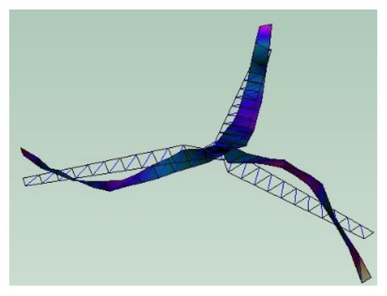
Figure 4.
Mode shape cloud diagram of the iced impeller.
4.2. Modal Result Analysis
Impeller modal tests were carried out on the ice-covered states F (0.7, 0.3, ∆m), F (0.35, 0.35, ∆m), F (0, 0.35, ∆m), and F (0, 1, ∆m), respectively. Each group was tested three times, and the average value of the three amounts was taken as the result. The first six-order natural frequencies of the impeller under different ice-covered states were obtained as shown in Table 1. To directly reflect the influence degree of icing on the natural frequency of the impeller, the change rate of natural frequency r is defined, as shown in Equation (22). The greater the absolute value of the change rate, the greater the influence of icing on the natural frequency of this order is:
where fi is the i-th-order natural frequency of the ice-free impeller. fj is the j-th-order natural frequency of the impeller after icing. i, j is 1, 2, 3, 4, 5, 6.

Table 1.
The first 6-order natural frequencies of impeller under different icing conditions.
The trend charts on the change rate of the first six-order natural frequencies under different icing states were obtained, as shown in Figure 5. It can be seen that the natural frequency change rate of the impeller presents different trends with different icing areas and icing quality. When the icing state is F (0.7, 0.3, ∆m), the natural frequency change rate of each order shows an increasing trend with the increase in icing quality. When the icing state is F (0.35, 0.35, ∆m), the change rate of the first-, second-, third-, and fourth-order natural frequencies increases with the increase in the ice-covered mass, and the change rate of the fifth- and sixt- order natural frequencies decreases negatively with the increase in the ice-covered mass. When the icing state is F (0, 0.35, ∆m), the change rate of the first, second-, third-, fourth- and fifth-order natural frequency increases with the increase in the ice-covered mass, and the change rate of the sixth-order natural frequency decreases negatively with the increase in the ice-covered mass. When the icing state is F (0, 1, ∆m), the change rates of the first-, second-, and third-order natural frequencies increase with the increase in the ice-covered mass, and the change rates of the fourth-, fifth-, and sixth-order natural frequencies decrease negatively with the increase in the ice-covered mass. Under different icing conditions, the absolute value of the natural frequency change rate of each order gradually increases, indicating that icing has a significant effect on each order of natural frequency.
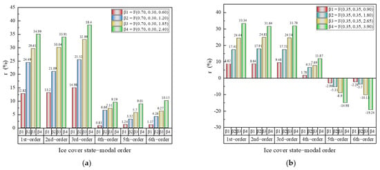
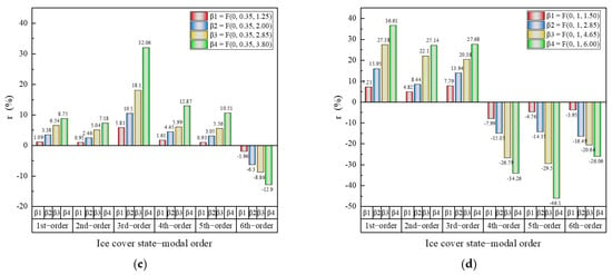
Figure 5.
Change rate trend of the natural frequency of impeller in the first 6 orders under different icing conditions. (a) F (0.7, 0.3, ∆m). (b) F (0.35, 0.35, ∆m). (c) F (0, 0.35, ∆m). (d) F (0, 1, ∆m).
At the same time, quadratic polynomials were used in Origin 2021 to fit the relationship between the covered-ice mass and the natural frequency change rate under different icing states. The quadratic polynomial fitting equations are shown in Table 2.

Table 2.
Quadratic fitting equation of the first 6 orders of natural frequency change rates of the impeller under different icing states.
As can be seen from Table 2, the correlation coefficients R2 of the fitting equations of each order are all greater than 0.93. This indicates that the fitting degree is good. Therefore, the fitting equation can be used to interpolate the corresponding natural frequency change rate of any icing mass between 0 and the maximum. In this section, the relationships between different ice-covering states and the change rates of each order of natural frequency are established, and the dataset of the deep neural network model is constructed by assigning different ice-covering quality values to each region.
5. Design of Deep Neural Network (DNN) Based on TensorFlow
5.1. TensorFlow Deep Learning Tool
TensorFlow is a second-generation open-source AI deep learning framework developed by Google that is based on disbelief. Tensor is the tensor of n-dimensional matrices, and Flow is the calculation based on the data flow graph, so TensorFlow is the calculation of n-dimensional matrices moving from one end of the data flow graph to the other. Due to its compatibility with Windows, Linux, and Mac systems, good cross-platform performance, portability, and high flexibility of the framework, TensorFlow has been widely used in deep learning fields such as speech recognition and image processing [21,22]. The Python language is used in this paper. A DNN algorithm based on the TensorFlow framework is developed experimentally.
5.2. DNN Neural Network Algorithm
A deep neural network (DNN), also known as a multi-layer perceptron (MLP), can be understood as a neural network with many hidden layers. It is an algorithm that realizes “multi-layer nonlinear transformation”. According to the positions of different layers, DNN can be divided into three categories: the input layer, the hidden layer, and the output layer, as shown in Figure 6. Generally speaking, the first layer is the input layer, the last layer is the output layer, and the middle layers are all hidden layers [23,24].
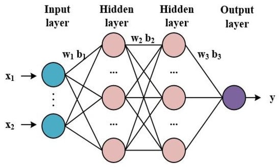
Figure 6.
DNN network architecture with three layers.
Neurons in the same layer are independent of each other and have no connection, and all layers are fully connected. That is, any neuron in the N-th layer must be connected to any neuron in the N + 1 layer. Although the DNN network looks very complex, it is still composed of a linear relationship and an activation function, just like a perceptron, from a small local model.
5.2.1. DNN Forward Propagation Algorithm
Forward propagation usually proceeds from local to global, and there is a certain correlation between the features of each local statistic. Several weight coefficient matrices w and bias vector b are used to carry out a series of linear operations and activation operations with the input value vector x. Starting from the input layer, the calculation proceeds back layer by layer, all the way to the output layer, until the output result is obtained [25].
5.2.2. DNN Back Propagation Algorithm
The core of back propagation is the loss function, which is used to measure the loss between the calculated output of training samples and the real output of training samples. We reverse to a series of weight coefficient matrix w and bias vector b, which are constantly updated until our expected effect is achieved. Generally, the mean square deviation function is chosen as the loss function measure. This minimizes the expectation of each sample. Finally, the output calculated by all training samples is equal to or close to the real value, as much as possible [26,27].
5.3. Prediction Model Construction for the Impeller Icing
To verify the effectiveness of the algorithm, the natural frequency change rate of the impeller under different ice-covered states was analyzed. The data samples were generated by the corresponding relation established above. The algorithm was developed in TensorFlow 2.2.0 under the Windows operating system, and the operating environment includes an Intel Core i3-2350M@1.60GHz processor with 12 GB of memory.
5.3.1. Data Pre-Processing
In this experiment, the data collected from the modal test of ice-covered impellers were analyzed. The quadratic fitting relationships established in the above section were used as the dataset. The dataset contains eight parameters, namely, the change rates of the first six-order natural frequencies for the ice-covered impeller, the ice-covered area, and the ice-covered quality. The dataset is selected and extracted using the Pandas function. At the same time, all data are normalized to minimize the error caused by the data difference [28], as shown in the following Equation:
where Tnorm is the normalized data, T is the original data, and Tmax and Tmin are the maximum and minimum values of the original data, respectively. Normalization is used to transform the data into a dimensionless numerical form within the interval [0, 1] to reduce the difference between values.
5.3.2. Model Design
The number of hidden layers and the number of nodes of neural networks have a great influence on the results of model training and prediction. Too many layers may lead to too long a training time and an over-fitting phenomenon, whereas too few layers may not meet the accuracy of the model. In this paper, after repeatedly adjusting parameters and the number of hidden layers and nodes, it was found that it is optimal to construct a DNN model with four hidden layers and a total of 512 nodes. The structure of the DNN prediction model is shown in Figure 7. In this study, the change rates of the first six-order natural frequencies of the impeller were selected as the input factor of the model, and the icing quality of different ice-covered areas was taken as the output of the model. When applying model prediction, input factors in the test set are input into the model, and then the prediction results of icing quality in different ice-covered areas are output. The model prediction process is shown in Figure 8, and the details are as follows.
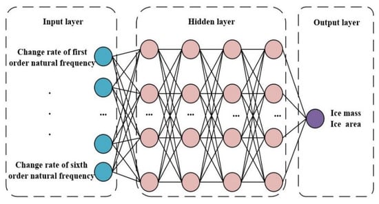
Figure 7.
Structure of DNN prediction model.
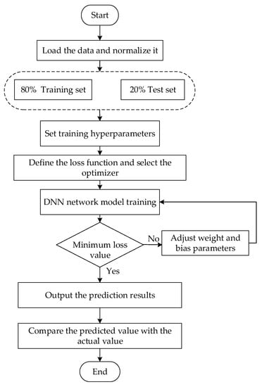
Figure 8.
Prediction model flow of ice coating quality of impeller.
First, modal tests were carried out on the impellers under different ice-covered conditions to obtain the original data.
Second, the data, such as the change rate of natural frequency, ice-covered area, and ice-covered quality, were normalized to eliminate the inconsistency of dimensional differences among the data.
Third, the dataset was divided by an 8:2 ratio. A total 80% of the data is used as the training set (20% of which is used as the validation set), and 20% of the data is used as the test set.
Fourthly, the model parameters are set, the network model is built, and training starts.
Finally, the loss value of the network model output is judged. If the loss value is reduced to the minimum, the training is finished. If the loss value is too high, the parameters are fine-tuned in reverse, and the model is retrained until the loss value decreases to 0. The training is completed, and the predicted value is output.
In this paper, six input factors and four hidden layers are designed, and the output layer is the icing quality under different icing areas of the impeller. The training parameter setup is shown in Table 3. Among them, the activation function Relu is a piecewise linear function [29]. Due to its simple calculation, it can alleviate the vanishing gradient problem caused by excessive network layers, and its model can be easily trained to obtain good performance. The Adam optimizer algorithm, which is easy to implement, can be adapted to carry out parameter optimization because of its low memory demand and high computational efficiency [30].

Table 3.
Parameter settings of DNN prediction model.
6. Results Analysis
6.1. Model Evaluation Index
In this paper, the mean absolute error (MAE) and the mean square error (MSE) were selected to evaluate the performance of the prediction model [31,32], and the expressions are shown in Equations (24) and (25). MAE is the average value of the absolute error between the predicted value and the actual value, which can avoid the error cancellation problem and accurately reflect the size of the actual prediction error. MSE is the expectation of the square difference between the actual value and the predicted value and takes the value [0, +∞). When the predicted value and the actual value are the same, MSE is 0:
where Pi is the predicted value and Ri is the real value.
The training effect of the model has a strong correlation with the order of the data. If there are regular sequential data in the training process, this may cause the model to fall into a local optimum and eventually lead to overfitting of the model. In order to avoid the impact of the fixed order of data input on the training results, this paper uses the shuffle function to shuffle the data before each iteration round to improve the model training effect.
In the process of model training, the changes in the saving loss function values (MAE and MSE) with the number of iterations are recorded in real time, as shown in Figure 9. It can be seen that all loss values decrease rapidly at the beginning, and after several iterations, the training and verification curves gradually smooth and begin approaching 0. This indicates that the model is constantly optimized and shows good prediction ability after multiple iterations of training.
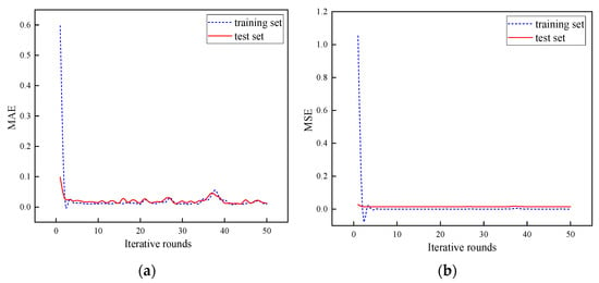
Figure 9.
The change curve of loss function with the number of iterations at (a) MAE. (b) MSE.
6.2. The Predicted Value Is Compared with the Real Value
The test set data were used for network model prediction. Four groups of samples were randomly selected under different icing states and imported into the trained DNN neural network model. The comparison between the predicted ice quality and the actual ice quality is shown in Figure 10, which can more intuitively reflect the prediction error between the predicted value of the DNN model and the actual value. Meanwhile, the relative error δ and the average error η are defined as shown in Equations (26) and (27) to describe the error of predicting ice quality. The error between the predicted value and the actual value under different icing conditions is shown in Table 4.
where is the actual ice-covered mass, and is the ice-covered mass predicted by the DNN model, i = 1, 2, 3, 4.
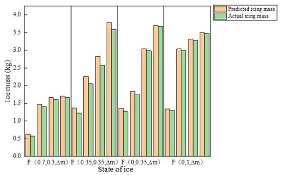
Figure 10.
Comparison between the predicted value and real value of ice coating mass of impeller.

Table 4.
Relative error of DNN model predicting ice mass.
It can be seen from Figure 10 and Table 4 that the DNN neural network model has a good predictive ability, and the predicted value is close to the actual value without participating in the training. The smaller the actual ice-covered mass of the impeller, the larger the relative error of the ice-covered mass predicted by the DNN model. For example, the actual ice-covered mass of the ice-covered state F (0.7, 0.3, 0.57) is 0.57 kg, the predicted ice-covered mass is 0.62 kg, and the relative error is 8.77%. In the same ice-covered state, the relative error will decrease gradually with the increase in ice-covered mass.
In the iced state F (0.7, 0.3, ∆m), F (0.35, 0.35, ∆m), F (0, 0.35, ∆m), F (0, 1, ∆m), the average prediction error of the DNN model is 4.79%, 9.35%, 3.62%, and 1.63%, respectively. It can be found that the ice-covered state F (0, 1, ∆m) has the smallest average error compared with the three other ice-covered states. That is, when all three blade surfaces of the impeller are ice-covered, the DNN model has the best prediction ability. In practice, when the wind turbine operates in cold weather, ice usually covers the surface of all three blades, and only a certain area of the blade surface is relatively bare. Therefore, the prediction accuracy of the DNN model established in this paper is high. That is, it can realize the precise prediction of the ice-covered quality of the impeller on the wind farm.
At present, the research on the icing problem of wind turbine blades focuses on the timely detection of blade icing and the removal of ice before impact, with such examples as the optical method, the infrared method, the ice sensor method, etc. However, most of these have limitations, such as limited application conditions and high costs. Nowadays, most wind turbines are equipped with blade vibration detection systems that include many sensors in the blade to collect the vibration signal of the blade. The change rate of the natural frequency can be obtained using the fast Fourier transform. The method presented in this paper can be used as the basis for designing a deicing system. Through deep neural network technology, the natural frequency change rate data of the wind turbine impeller are analyzed, and the neural network is trained to obtain an icing prediction model, so as to achieve the purpose of early icing prediction, leading to deicing the wind turbine blades in time to eliminate hidden dangers. The final example shows that the DNN neural network method can effectively predict the icing mass, and the error is lower than that of the methods proposed by Gantasala [33] and Li [34]. It shows good prediction accuracy and generalization ability. It provides a new idea for the fault diagnosis of and deicing decisions for wind turbine blades.
7. Conclusions
In this paper, a blade icing test was carried out in a natural environment, and a modal test was realized using B&K modal test instruments and PULSE16.1.1 modal analysis software aiming at a 600 W small wind turbine impeller. The corresponding relationships between the icing mass and the natural frequency change rate under different icing states were established. The DNN neural network was also applied to predict the icing mass of the impeller. The following conclusions were obtained.
First, the force-hammer modal tests of the impeller with ice-coated blades showed that icing has a great influence on each natural frequency of the wind turbine impeller under different icing states, and the absolute value of the natural frequency change rate increases with the increase in ice-coated mass. The corresponding relationships between the icing mass and the change rate of the first six-order natural frequencies were established, and the correlation coefficients were all beyond 0.93. This indicates that there is an obvious quantitative relationship between the natural frequency change rate and the ice-coated mass in different areas, which can be used to diagnose the icing situation in engineering practice.
Secondly, the deep neural network (DNN) prediction model of ice-coating quality for the impeller was constructed with the change rates of the first six-order natural frequencies as the input factors. The results showed that the MAE and MSE of the trained model were close to 0. The average prediction error of the DNN model was 4.79%, 9.35%, 3.62%, 1.63%, respectively, under different icing states of the impeller. It can be seen that the DNN shows better prediction ability than other methods. The smaller the actual ice-coated mass of the impeller, the larger the relative error of the ice-coated mass predicted by the DNN model. In the same icing state, the relative error will decrease gradually with the increase in ice-coated mass. In a word, it is more feasible and accurate to use the natural frequency change rate to predict the icing quality.
Author Contributions
Conceptualization, H.C. and Z.L.; methodology, Z.L. and H.C.; software, Z.L. and H.C.; validation, B.S., Y.L. and L.L.; data curation, T.F. and J.W.; writing—original draft preparation, Z.L. and H.C.; writing—review and editing, Z.L. and H.C.; project administration, H.C. and Y.Z.; funding, H.C. All authors have read and agreed to the published version of the manuscript.
Funding
This work was supported by a project from National Natural Science Foundation of China (grant No. 12064033), a project from the Interdisciplinary Research Fund of Inner Mongolia Agricultural University (grant No. BR22-15-07), a project from the Science and Technology Plan of Inner Mongolia Autonomous Region in China in 2020 (grant No. 2020GG0314), and a project from the Talent Fund of Inner Mongolia Autonomous Region in 2021.
Data Availability Statement
Not applicable.
Acknowledgments
The authors would like to thank the anonymous reviewers who gave valuable suggestions that have helped to improve the quality of the manuscript.
Conflicts of Interest
The authors declare no conflict of interest.
References
- Aizpurua-Etxezarreta, M.; Carreno-Madinabeitia, S.; Ulazia, A.; Sáenz, J.; Saenz-Aguirre, A. Long-Term Freezing Temperatures Frequency Change Effect on Wind Energy Gain (Eurasia and North America, 1950–2019). Sustainability 2022, 14, 5630. [Google Scholar] [CrossRef]
- Fakorede, O.; Feger, Z.; Ibrahim, H.; Ilinca, A.; Perron, J.; Masson, C. Ice protection systems for wind turbines in cold climate: Characteristics, comparisons and analysis. Renew. Sustain. Energy Rev. 2016, 65, 662–675. [Google Scholar] [CrossRef]
- Awada, A.; Younes, R.; Ilinca, A. Review of Vibration Control Methods for Wind Turbines. Energies 2021, 14, 3058. [Google Scholar] [CrossRef]
- Li, Y.; Sun, C.; Jiang, Y.; Feng, F. Scaling Method of the Rotating Blade of a Wind Turbine for a Rime Ice Wind Tunnel Test. Energies 2019, 12, 627. [Google Scholar] [CrossRef]
- Lamraoui, F.; Fortin, G.; Benoit, R.; Perron, J.; Masson, C. Atmospheric icing impact on wind turbine production. Cold Reg. Sci. Technol. 2014, 100, 36–49. [Google Scholar] [CrossRef]
- Alsabagh, A.S.; Xu, Y.; Virk, M.S.; Badran, O. Atmospheric Ice Loading and its Impact on Natural Frequencies of Wind Turbines. Wind Eng. 2015, 39, 83–96. [Google Scholar] [CrossRef]
- Jin, J.Y.; Virk, M.S. Study of ice accretion and icing effects on aerodynamic characteristics of DU96 wind turbine blade profile. Cold Reg. Sci. Technol. 2019, 160, 119–127. [Google Scholar] [CrossRef]
- Gantasala, S.; Tabatabaei, N.; Cervantes, M.; Aidanpää, J.-O. Numerical Investigation of the Aeroelastic Behavior of a Wind Turbine with Iced Blades. Energies 2019, 12, 2422. [Google Scholar] [CrossRef]
- Yirtici, O.; Cengiz, K.; Ozgen, S.; Tuncer, I.H. Aerodynamic validation studies on the performance analysis of iced wind turbine blades. Comput. Fluids 2019, 192, 104271. [Google Scholar] [CrossRef]
- Manatbayev, R.; Baizhuma, Z.; Bolegenova, S.; Georgiev, A. Numerical simulations on static Vertical Axis Wind Turbine blade icing. Renew. Energy 2021, 170, 997–1007. [Google Scholar] [CrossRef]
- Huang, C.; Ye, L.; Ge, J.; Zhou, C. Experimental Study on Wind Turbine Blade Icing Detection System. Instrum. Tech. Sens. 2014, 6, 86–88+92. [Google Scholar]
- Davis, N.N.; Byrkjedal, Ø.; Hahmann, A.N.; Clausen, N.-E.; Žagar, M. Ice detection on wind turbines using the observed power curve. Wind Energy 2015, 19, 999–1010. [Google Scholar] [CrossRef]
- Skrimpas, G.A.; Kleani, K.; Mijatovic, N.; Sweeney, C.W.; Jensen, B.B.; Holboell, J. Detection of icing on wind turbine blades by means of vibration and power curve analysis. Wind Energy 2016, 19, 1819–1832. [Google Scholar] [CrossRef]
- Ningbo, L.I.; Tao, Y.; Naipeng, L.; Detong, K.; Qingchao, L.; Yaguo, L. Ice Detection Method by Using SCADA Data on Wind Turbine Blades. Power Gener. Technol. 2018, 39, 58–62. [Google Scholar] [CrossRef]
- Yang, X.; Ye, T.; Wang, Q.; Tao, Z. Diagnosis of Blade Icing Using Multiple Intelligent Algorithms. Energies 2020, 13, 2975. [Google Scholar] [CrossRef]
- Guo, P.; Infield, D. Wind turbine blade icing detection with multi-model collaborative monitoring method. Renew. Energy 2021, 179, 1098–1105. [Google Scholar] [CrossRef]
- Kabardin, I.; Dvoynishnikov, S.; Gordienko, M.; Kakaulin, S.; Ledovsky, V.; Gusev, G.; Zuev, V.; Okulov, V. Optical Methods for Measuring Icing of Wind Turbine Blades. Energies 2021, 14, 6485. [Google Scholar] [CrossRef]
- Cao, S.; Zhang, W.; Xiao, L. Theoretical Experiment and Application of Vibration Structure Modal Analysis, 2nd ed.; Tianjin University Press: Tianjin, China, 2014; ISBN 978-7-5618-5153-1. [Google Scholar]
- Heylen, W.; Lamriens, S.; Sas, P. Modal Analysis Theory and Testing; Beijing University of Technology Press: Beijing, China, 2001; ISBN 7-81045-797-7. [Google Scholar]
- Liu, S.; Li, L.; Yu, T.; Lei, L.; Li, M. Diagnosis Technology for the Icing Status of Wind Turbine Blades Based on Vibration Detection. Chin. J. Electr. Eng. 2013, 33, 88–95. [Google Scholar] [CrossRef]
- Xu, W. The Realization and Optimization Technology of Recognition Algorithm Based on Tensorflow Deep Learning Mechanism. J. Phys. Conf. Ser. 2021, 2066, 012002. [Google Scholar] [CrossRef]
- Su, Y.; Yang, J.; Dai, X.; Liu, J.; Hou, X. TensorFlow Neural Network Based Load and Mutual Inductance Identification Method for Magnetic Coupling Resonant Wireless Power Transfer System. Power Syst. Autom. 2021, 45, 162–169. [Google Scholar] [CrossRef]
- Alotaibi, M.A. Machine Learning Approach for Short-Term Load Forecasting Using Deep Neural Network. Energies 2022, 15, 6261. [Google Scholar] [CrossRef]
- Sok, V.; Lee, S.-W.; Kang, S.-H.; Nam, S.-R. Deep Neural Network-Based Removal of a Decaying DC Offset in Less than One Cycle for Digital Relaying. Energies 2022, 15, 2644. [Google Scholar] [CrossRef]
- Ansari, S.; Ayob, A.; Lipu, M.S.H.; Hussain, A.; Saad, M.H.M. Data-Driven Remaining Useful Life Prediction for Lithium-Ion Batteries Using Multi-Charging Profile Framework: A Recurrent Neural Network Approach. Sustainability 2021, 13, 13333. [Google Scholar] [CrossRef]
- Wright, L.G.; Onodera, T.; Stein, M.M.; Wang, T.; Schachter, D.T.; Hu, Z.; McMahon, P.L. Deep physical neural networks trained with backpropagation. Nature 2022, 601, 549–555. [Google Scholar] [CrossRef] [PubMed]
- Thango, B.A.; Bokoro, P.N. Prediction of the Degree of Polymerization in Transformer Cellulose Insulation Using the Feedforward Backpropagation Artificial Neural Network. Energies 2022, 15, 4209. [Google Scholar] [CrossRef]
- Djordjević, L.; Jordović-Pavlović, M.I.; Ćojbašić, M.; Galović, S.P.; Popović, M.N.; Nešić, M.V.; Markushev, D.D. Influence of data scaling and normalization on overall neural network performances in photoacoustics. Opt. Quantum Electron. 2022, 54, 501. [Google Scholar] [CrossRef]
- Kim, Y.; Ohn, I.; Kim, D. Fast convergence rates of deep neural networks for classification. Neural Netw. 2021, 138, 179–197. [Google Scholar] [CrossRef]
- Solgi, R.; Loáiciga, H.A.; Kram, M. Long short-term memory neural network (LSTM-NN) for aquifer level time series forecasting using in-situ piezometric observations. J. Hydrol. 2021, 601, 126800. [Google Scholar] [CrossRef]
- Chicco, D.; Warrens, M.J.; Jurman, G. The coefficient of determination R-squared is more informative than SMAPE, MAE, MAPE, MSE and RMSE in regression analysis evaluation. PeerJ Comput. Sci. 2021, 7, e623. [Google Scholar] [CrossRef]
- Zhang, H.; Jing, Y.; Zhao, Y. FS-LSTM: Sales forecasting in e-commerceon feature selection. J. China Univ. Posts Telecommun. 2022, 29, 92–98. [Google Scholar] [CrossRef]
- Gantasala, S.; Luneno, J.-C.; Aidanpää, J.-O. Identification of ice mass accumulated on wind turbine blades using its natural frequencies. Wind Eng. 2017, 42, 66–84. [Google Scholar] [CrossRef]
- Li, F.; Cui, H.; Su, H.; Iderchuluun; Ma, Z.; Zhu, Y.; Zhang, Y. Icing condition prediction of wind turbine blade by using artificial neural network based on modal frequency. Cold Reg. Sci. Technol. 2021, 194, 103467. [Google Scholar] [CrossRef]
Publisher’s Note: MDPI stays neutral with regard to jurisdictional claims in published maps and institutional affiliations. |
© 2022 by the authors. Licensee MDPI, Basel, Switzerland. This article is an open access article distributed under the terms and conditions of the Creative Commons Attribution (CC BY) license (https://creativecommons.org/licenses/by/4.0/).