Article

Short-Term Electricity Price Forecasting Based on the Two-Layer VMD Decomposition Technique and SSA-LSTM

1
School of Mechatronical Engineering and Automation, Foshan University, Foshan 528231, China
2
Yangtze Delta Region Institute, University of Electronic Science and Technology of China, Huzhou 313098, China
3
School of Information, Xuzhou Vocational College of Industrial Technology, Xuzhou 221140, China
*
Author to whom correspondence should be addressed.
Energies 2022, 15(22), 8445; https://doi.org/10.3390/en15228445
Submission received: 18 October 2022 / Revised: 9 November 2022 / Accepted: 10 November 2022 / Published: 11 November 2022

Abstract

:
Accurate electricity price forecasting (EPF) can provide a necessary basis for market decision making by power market participants to reduce the operating cost of the power system and ensure the system’s stable operation. To address the characteristics of high frequency, strong nonlinearity, and high volatility of electricity prices, this paper proposes a short-term electricity price forecasting model based on a two-layer variational modal decomposition (VMD) technique, using the sparrow search algorithm (SSA) to optimize the long and short-term memory network (LSTM). The original electricity price sequence is decomposed into multiple modal components using VMD. Then, each piece is predicted separately using an SSA-optimized LSTM. For the element with the worst prediction accuracy, IMF-worst is decomposed for a second time using VMD to explore the price characteristics further. Finally, the prediction results of each modal component are reconstructed to obtain the final prediction results. To verify the validity and accuracy of the proposed model, this paper uses data from three electricity markets, Australia, Spain, and France, for validation analysis. The experimental results show that the proposed model has MAPE of 0.39%, 1.58%, and 0.95%, RMSE of 0.25, 0.9, and 0.3, and MAE of 0.19, 0.68, and 0.31 in three different cases, indicating that the proposed model can well handle the nonlinear and non-stationarity characteristics of the electricity price series and has superior forecasting performance.

1. Introduction

Electric energy can be traded freely in a market similar to other common commodities in the electricity market. Electricity prices, which can reflect electricity supply and demand, have become an essential element in the electricity market [1]. In recent years, many researchers have demonstrated that it is difficult to forecast accurately because electricity prices depend heavily on various factors [2,3]. As a special commodity, the price of electricity usually exhibits complex characteristics such as seasonality, calendar effects, non-stationarity, non-linearity, and mean reversion [4]. Combined with the fact that electricity can not be stored on a large scale and must meet the balance of supply and demand at all times, electricity prices are highly volatile and often accompanied by extreme spikes [5,6]. As decentralized commercial entities replace vertically integrated electric utilities, more market players face fierce competition [7]. Accurate EPF not only enhances the efficiency of the market in regulating the allocation of energy resources and improves the optimal dispatch of the grid, but also provides an essential basis for all market participants to make and adjust market decisions and thus obtain corresponding economic benefits [8]. Therefore, accurate EPF is necessary for the whole power system and market participants. There are numerous methods for EPF. In recent years, scholars have conducted extensive research on the methods of EPF. According to the literature [9], the main methods of EPF are econometric models [10,11,12], deep learning methods, and hybrid models.
Econometric models generally use econometric models for forecasting, mainly including autoregressive moving average (ARMA), autoregressive integrated moving average (ARIMA), and generalized autoregressive conditional heteroskedasticity (GARCH). Most traditional econometric models combine historical and current data through mathematical methods, so their fitting effect on electricity price series is not good [13]. Some researchers have combined econometric models with other methods to improve their forecasting ability. The literature [14] proposes a forecasting method with wavelet transform combined with ARIMA and GARCH. In the literature [15], Zhang et al. propose a hybrid forecasting method combining wavelet transform, adaptive particle swarm optimization kernel limit learning machine (SAPSO-KELM) and ARMA. The literature [16] proposes an integrated forecasting model based on IEMD, ARMAX-EGARCH, and ANFIS, which uses different treatments for the linear and nonlinear components of electricity prices. However, econometric models are more limited in capturing electricity prices’ nonlinear and highly volatile characteristics, and they make it difficult to deal with complex or nonlinear time series problems.
Deep learning methods combine elements of learning, fuzziness, and superior performance in electricity price prediction problems by creating systems capable of adapting to complex dynamic changes, making them immensely popular in EPFs in recent years. Deep learning methods mainly contain artificial neural networks (ANN) [17,18,19], deep neural networks (DNN) [20], support vector machines (SVM) [21,22,23], and other methods [24,25]. Among them, SVM makes it difficult to deal with large-scale data, ANN makes it easy to overlearn and fall into local optimum, and its generalization ability needs to be improved. DNNs are subdivided into three main categories: feedforward neural networks (FNN) [26,27], recurrent neural networks (RNN) [28], and convolutional neural networks (CNN) [29,30,31,32]. These methods can approximate any multivariate function to the desired accuracy by adjusting the weights during online updates and can capture the complex, dynamic, and nonlinear features of electricity prices [15].
Among them, RNNs obtain excellent performance in time series prediction by constructing additional mappings to preserve relevant information from past inputs and apply it to the computation of current outputs. However, RNNs can suffer from gradient disappearance or gradient explosion after multi-stage propagation, known as the long-term dependence problem. The Long Short-Time Neural Network (LSTM) is an essential variant of RNN, which introduces memory units based on the traditional RNN structure and solves the gradient vanishing and gradient explosion problems well. The inclusion of memory units makes LSTM more adept at discovering and exploiting the intrinsic patterns of long sequence data, and it has been widely used in electricity price prediction. In the literature [33], Lu et al. proposed a differential evolutionary algorithm to optimize the forecasting model of LSTM and compared it with various models such as ANN and SVR. In the literature [34], a prediction model using an enhanced particle swarm algorithm to optimize LSTM was proposed and applied to forecast the closing price of the Indian energy exchange. In the literature [7], Li et al. use LSTM combined with a feature selection algorithm to predict electricity prices considering market coupling, and finally, use the electricity price data of the Nordic electricity market to verify it. However, none of the above methods can solve the nonlinear and non-stationarity characteristics of electricity prices well.
The approach that has received the most scholarly attention in the past few years is the hybrid model. Hybrid models generally consist of a combination of data processing or feature extraction methods combined with one or more predictive models [15,16,35,36,37,38,39,40,41,42,43,44]. Due to the volatility and nonlinearity of electricity prices, many researchers would combine some data decomposition techniques to preprocess the electricity price series to further improve the model’s prediction accuracy. Among the existing decomposition methods, WT [13,14,15] and empirical modal decomposition (EMD) [45,46,47] have been widely used. Although EMD can achieve better results than WT, it has an end effect that will affect the accuracy of EMD decomposition [48]. Some researchers have addressed this problem by improving the EMD. For example, in the literature [16], Zhang used an improved empirical modal decomposition (IEMD). As well as in the literature [49], Jiang used fast integrated empirical modal decomposition (FEEMD). However, EMD also has the problem of modal mixing, which will harm the decomposition effect of EMD. To overcome the end effects and modal aliasing in EMD, scholars have introduced variational modal decomposition (VMD) [50,51]. VMD uses non-recursive theory to decompose the signal, which has better robustness and improves the modal aliasing problem. However, although a single decomposition technique can improve the predictive accuracy to some extent, it is often difficult for a single decomposition technique to completely deal with the irregularity and non-stationarity of the electricity price series.
This paper introduces a two-layer VMD technique to improve the model’s prediction capability to further address this problem. Considering the excellent performance of LSTM in time series prediction and the advantages of VMD in processing signals, this paper proposes a hybrid model based on a two-layer VMD decomposition technique and a sparrow search algorithm (SSA) to optimize LSTM. Firstly, the original electricity price sequence is decomposed into multiple eigenmode functions (IMFs) with different center frequencies by VMD. In the second step, the network structure parameters of the LSTM are optimized using SSA, and each IMF component is predicted separately using the optimized LSTM. In the third step, the prediction accuracy of each IMF is evaluated. The IMF-worst with the worst prediction accuracy is decomposed for the second time using VMD. Then, the second prediction is performed using SSA-optimized LSTM to obtain the predicted value of IMF-worst. Finally, the prediction values of all IMFs are cumulatively reconstructed to get the final prediction values.
This paper’s main innovations and contributions can be mentioned in the following aspects: (1) This paper presents a hybrid model for electricity price prediction based on a two-layer VMD technique and SSA-optimized LSTM. The two-layer VMD decomposition technique is introduced for the characteristics of non-stationarity and non-linearity of electricity price series. (2) SSA is used to optimize the LSTM and find the appropriate network structure parameters for the LSTM to improve the model’s predictive power. (3) Electricity price data from three electricity markets in New South Wales, Australia, Spain, and France are used, allowing a comprehensive and systematic assessment of the validity and accuracy of the proposed model. The results of the experiments show that the proposed model has a better forecasting effect than other considered models. It is necessary to state that in actual engineering practice, data of other variables such as temperature and load are often difficult to obtain. Therefore, this paper tries to investigate a prediction method based on historical electricity price data for the characteristics of nonlinearity, non-stationarity, and high volatility of electricity price, and adapt to the electricity price prediction in the scenario where data for other variables are not available.
The remainder of the paper is organized as follows: Section 2 introduces the basic theoretical approach. Section 3 describes the framework of the model. Section 4 presents the case study results. Section 5 provides some discussion and conclusions.

2. Methodology

2.1. Variational Mode Decomposition(VMD)

The literature [52] demonstrated that the decomposition of the original sequence into multiple subsequences helps improve prediction results’ accuracy. VMD is an entirely non-recursive adaptive variational pattern decomposition approach proposed by Dragomiretskiy et al. [53]. Its core idea mainly involves the construction and solution of variational models. The method assumes that all components of a sequence signal are narrowband signals concentrated around their respective center frequencies. In the process of obtaining the decomposed components, a constrained optimization problem is established according to the narrowband conditions of the details. Each element’s frequency center and bandwidth are determined by iteratively searching for the optimal solution of the variational model so that the frequency domain dissection of the sequence signal and the effective separation of each component can be realized adaptively. The original electricity price sequence can be decomposed into several modal components with different center frequencies after VMD. In this way, the complex original electricity price can be transformed into a set of relatively stable and more regular subsequences, which provide more apparent features of the electricity prices in different frequency domains, making it easier for the neural network to learn.
Assuming that each modal component is a finite bandwidth with central frequency ω k , the variational problem can be described as seeking K-modal functions u k t such that the sum of the estimated bandwidths of each mode is minimized. The constraint is that the sum of each modal is equal to the input signal f . The VMD model is constructed in the following steps.
(1) The analytic signal of each modal function u k t is obtained using the Hilbert transform to get its one-sided spectrum.
(2) The resolved signal of each modal is mixed with the corresponding center frequency, e j ω k t , so that the spectrum of each mode is modulated to the corresponding fundamental frequency band.
(3) The signal is demodulated according to the Gaussian smoothness and the quadratic criterion of the gradient, and the quadratic L2 norm of the gradient is calculated to obtain the bandwidth of each decomposed mode.
The variational constraint model is obtained as follows:
k = 1 K t δ t + j π t u k t e j ω k t 2 2 u k ω k m i n   ,   s . t . k u k = f  
where t is the partial derivative operator; δ t is the Dirac distribution function; 1/(πt) is the shock response; u k is the modal component; and f is the original sequence signal. To solve the above model, a quadratic penalty factor α and a Lagrange multiplier operator λ are introduced to transform the constrained variational problem into an unconstrained variational problem with the following expressions:
L u k , ω k , λ : = α k = 1 K t [ ( δ t + j π t ) u k t ] e j ω k t 2 2 + f t k = 1 K u k t 2 2 + λ t , f t k = 1 K u k t ,
the alternate direction method of multipliers (ADMM) deals with the above unconstrained variational problem. The variational modal optimal solution in Equation (1) is solved by alternately updating u k n + 1 , ω k n + 1 , and λ k n + 1 (n is the number of iterations). The new u k and the central frequency ω k are:
u ^ k n + 1 ω = f ^ ω i k u ^ i n ω + λ ^ ω 2 1 + 2 α ω ω k 2 ,
ω k n + 1 = 0 ω u ^ k n + 1 ω 2 d ω 0 u ^ k n + 1 ω 2 d ω ,
where f ^ ω , u ^ i ω , λ ^ ω are the Fourier transforms of the points f t , u i t , and λ t , respectively.

2.2. Sparrow Search Algorithm (SSA)

The sparrow search algorithm (SSA) is a population intelligence optimization algorithm proposed by Jiankai Xuea et al. in 2020 [54], which has the advantages of global foraging, few adjustable parameters, and a clear structure. The algorithm builds a mathematical model based on the foraging behavior of sparrows. It incorporates a detection mechanism, where some sparrows in the population are randomly selected as scouts to establish an anti-predation mechanism. Each sparrow is a particle in the search space and represents a solution to the problem. Sparrows at the edge will update their position toward the center of the population to avoid danger, whereas sparrows at the center of the people will perform random wandering.
During foraging, a population of n sparrows in d-dimensional space can be expressed as:
X = x 1 1   x 1 2     x 1 d x 2 1   x 2 2     x 2 d       x n 1   x n 2     x n d ,
the fitness values for all sparrows can be expressed as:
F x = f x 1 1   x 1 2       x 1 d f x 2 1   x 2 2       x 2 d       f x n 1   x n 2       x n d
Sparrow populations have producers and scroungers. The producer has a high fitness value and can provide all scroungers with foraging directions and areas to guide the population in their search. There is a dynamic change between the two identities of individual sparrows, and each sparrow can become a producer if it finds a better food source. The shift in fitness value determines whether the scrounger follows the producer.
In each iteration of the optimization search process, the producer’s position is updated with the formula:
X i , j t + 1 = X i , j t · exp i α · T m a x ,     if   R 2 < S T X i , j t + Q · L   ,     if   R 2 S T ,  
where t is the number of iterations; T m a x is the maximum number of iterations; α is a random number uniformly distributed between (0, 1]; Q is a random number obeying a positive-terrestrial distribution; and L is a 1 × d matrix with each element inside being 1. When R 2 < ST, there is no danger around the sparrow population. The producer can search extensively for physical objects and lead other individuals to obtain a higher fitness value. When R 2 ≥ ST, scouts find danger approaching, and will signal danger and trigger anti-predatory behavior. Meanwhile, the producer will lead scroungers to perform position updates to safer areas for foraging. The position of scroungers is updated as follows:
X i , j t + 1 = Q · exp X w o r s t t X i , j t i 2   ,       if   i > n / 2 X P t + 1 + X i , j t X P t + 1 · A + · L ,     otherwise ,
where X w o r s t t denotes the current global worst position; X P t + 1 denotes the producer occupy the optimal position; and A is a multidimensional matrix with elements of 1 or −1 and satisfies A + = A T A A T 1 . When i > n/2, it suggests that the ith sparrow has too low an adaptation value and needs to fly to other areas to forage. When in/2, it means that the ith sparrow will feed randomly around the position of the current producer X P t + 1 .
The scout is responsible for monitoring the foraging area and will immediately signal danger when it is aware of approaching danger. At the same time, it will quickly move to a safe area or randomly approach other individual sparrows to reduce the likelihood of predation. The scout’s position update formula can be expressed as follow:
X i , j t + 1 = X b e s t t + β · X i , j t X b e s t t   ,     if   f i > f g X i , j t + k · X i , j t X w o r s t t f i f ω + ε   ,   if     f i = f g
where X b e s t t is the current global optimal position; β is the step control parameter, which obeys a normal distribution with mean 0 and variance 1; f i , f ω , f g are the current individual fitness value, global worst, and optimal fitness values, respectively; k ∈ [−1, 1] is used to control the direction of sparrow movement; and ε is a minimum value that is not zero. When f i > f g , it suggests that the sparrow is at the edge of the population and is highly vulnerable to predators. When   f i = f g , the sparrow is in the middle of the population and aware of the danger. The sparrow will move closer to other individuals to protect itself from predators.

2.3. Long Short-Term Memory Neural Network (LSTM)

Traditional recurrent neural networks have good performance in processing time series style by combining the temporality of data with network design but are prone to gradient disappearance and gradient explosion problems when dealing with long-time span nonlinear data. LSTM improves the traditional recurrent neural network structure by introducing memory units to control information transfer, effectively solving the long-term temporal dependence between data [55]. The memory unit can prevent the information from transferring based on the current input. The memory unit can determine the probability of allowing the information to pass based on the current input and the previous hidden state. This enables the whole network to remember and forget the data, which gives LSTM a great advantage when dealing with long time series such as electricity price series.
The LSTM consists of multiple LSTM cells. The LSTM cells include forgetting gates, input, and output gates, as shown in Figure 1. These three gates are used to learn the history input, current input, and history output in a weighted manner to achieve the memory function. The forgetting gate reads the output ht−1 of the previous cell and the current input xt via Sigmoid nonlinear mapping to selectively remember and forget information. The input gate determines the information stored in the recent memory cell state Ct. The output gate then determines the output information ht based on the current new cell state Ct.
The updated formula for Ct and ht within the LSTM cell is as follow:
f t = σ W f · h t 1 , x t + b f ,
i t = σ W i · h t 1 , x t + b i ,
C ˜ t = t a n h W C · h t 1 , x t + b C ,
C t = f t C t 1 + i t C ˜ t ,
o t = σ W o · h t 1 , x t + b o ,
h t = o t t a n h C t ,
where f t , i t , o t , C t , and h t denote the values of the forgetting gate state, input gate state, output gate state, memory cell, and hidden state at the moment t, respectively; σ is the Sigmoid activation function; W f , W i , and W C are the weight matrices of the forgetting gate, input gate, and output gate, respectively; and b f , b i , and b C are the deviation matrices of the forgetting gate, input gate, and output gate, respectively.

2.4. Normalization and Denormalization

To make the data fit the model better to improve the model’s prediction effect, the decomposed modal components need to be normalized. This paper uses the Min-max normalization method to normalize the data set to the range of 0 to 1. The Min-max normalization method is a linear transformation of the original data. Let minA and maxA be the minimum and maximum values of the data set A. The original value x of A is normalized to the value x′ in the interval [0, 1] by Min-max normalization. The normalization formula is as follows:
x = x m i n A m a x A m i n A ,  
After the SSA-LSTM prediction, the prediction result of each subsequence is obtained, which needs to be inverse normalized and then cumulatively reconstructed to obtain the final prediction result. The inverse normalization formula is as follow:
Y = y m a x A m i n A + m i n A ,
where y is the subseries predicted value and Y is the actual expected value after inverse normalization.

3. Construction of VMD-SSA-LSTM Model

3.1. Input and Output of the Model

The proposed method in this paper uses historical electricity price data as the input to the model. Before inputting into the model, the original prices sequence is divided into two parts, the training set and the test set, which are decomposed by a two-layer VMD decomposition technique and then transformed into a supervised learning form to be input into the model for one-step-ahead prediction. After several experimental comparisons, the data is finally fed into the model in the form of t-3, t-2, and t-1 prices to predict the electricity price at time t. The output of the model is the predicted value of each modal component, and the final predicted value is obtained after reconstruction.

3.2. Two-Layer VMD Decomposition Technique

In the electricity market, the electricity price is characterized by non-linearity, non-stationarity and high volatility, and is often accompanied by some extreme electricity prices. To cope with this problem, we propose a two-layer VMD decomposition technique based on the single decomposition approach. Firstly, the original electricity price series are decomposed adaptively using VMD decomposition. In this process, the complex features contained in the original prices are decomposed into multiple relatively stable modal components, and the extreme prices are also included. These modal components provide clearer temporal characteristics of the electricity prices in each frequency domain, which can be more easily learned by the neural network. After the first layer decomposition, we find that some high-frequency components often contain rich prices features that are not extracted. These features are hidden in high-frequency noise and are difficult to be detected. A single decomposition approach often performs poorly in the face of this problem. Therefore, we evaluate each component obtained after the first decomposition, and obtain the IMF-worst component with the worst prediction accuracy, i.e., the component that contains the most information. Then, we use the second VMD decomposition for IMF-worst to further extract the prices features contained in it to improve the prediction accuracy for this component, and thus improve the prediction accuracy of the whole model.

3.3. SSA Optimize LSTM’s Hyperparameters

The model parameters of LSTM, such as the number of neurons in the hidden layer and the number of iterations, significantly impact the accuracy of the electricity price prediction results. Therefore, the hyperparameters of the LSTM model need to be optimized to find the most suitable network parameters. SSA shows good convergence speed and accuracy performance and has some advantages in dealing with nonlinear problems. Thus, this paper uses SSA to optimize the hyperparameters, such as the number of cells in the hidden layer and the number of iterations of the LSTM model. The optimization steps are as follows:
(1) Determine the number of sparrow populations, the proportion of discoverers, the finding dimension, the number of optimization iterations, and the parameter thresholds. Sort and classify the sparrow population and initialize the SSA.
(2) Sparrow positions are updated by the producer, scrounger, and warning condition formulas. The predicted values of the LSTM and the root mean square of the sample data are used to determine the fitness values of the sparrow population. The optimal individual positions and global optimal position values in the population are saved.
(3) Judge whether the sparrow best adaptation in this iteration is better than the global best adaptation. If yes, exit the loop and return the optimal individual solution, i.e., determine the LSTM optimal hyperparameters. Otherwise, continue the loop iteration to find the optimal until the number of update iterations reaches the maximum.

3.4. Forecasting Process of VMD-SSA-LSTM Model

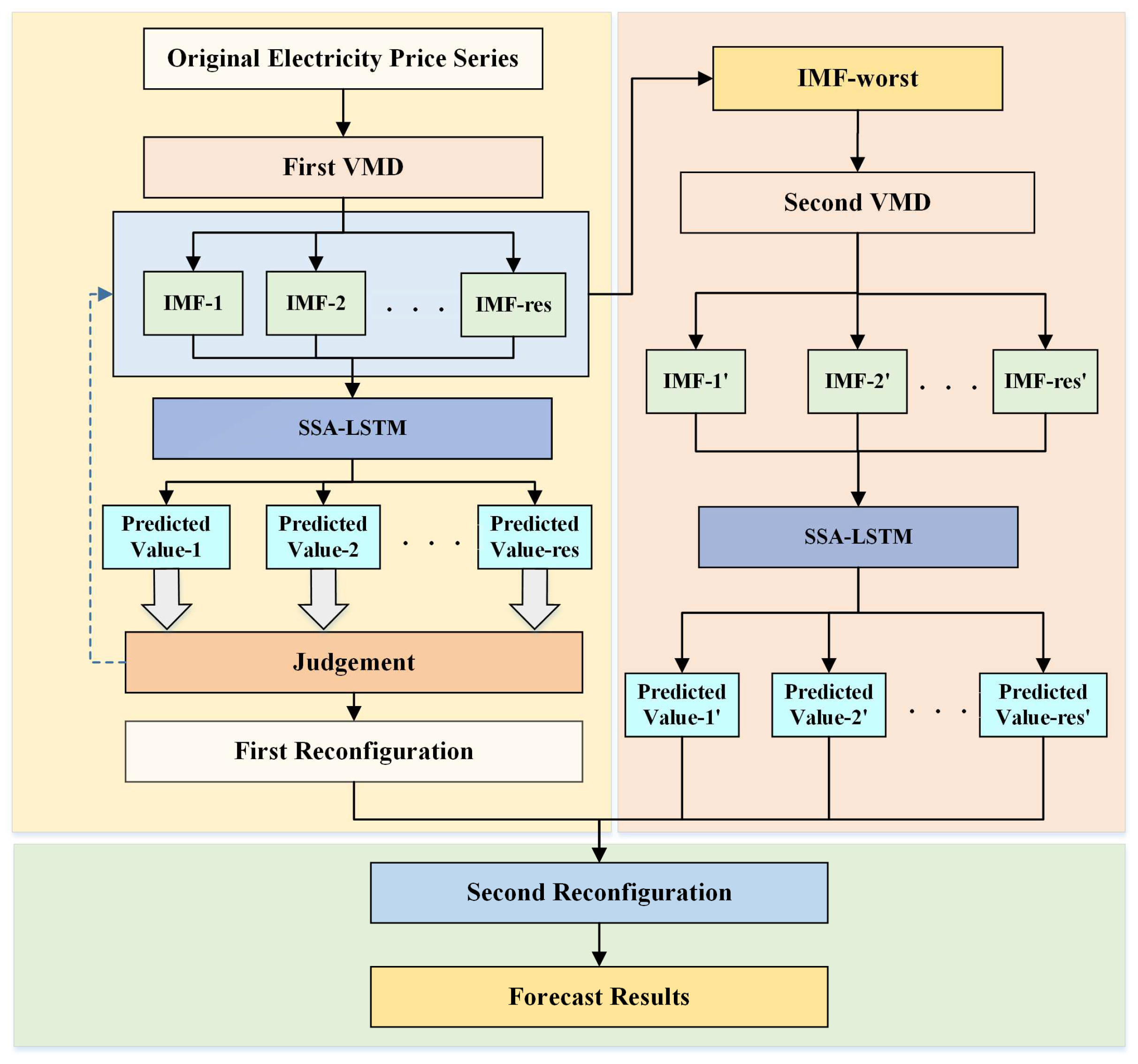
As mentioned above, the electricity price series has complex characteristics such as high frequency, nonlinearity, and volatility, which brings no small challenge to the accurate prediction of electricity prices. The VMD decomposition technique can decompose the complex electricity price signal into several standard modal components, thus significantly improving the prediction accuracy. In addition, LSTM has an excellent ability to deal with long-time series problems. Therefore, this paper combines the dual advantages of VMD and LSTM. SSA is used to optimize the network structure parameters of LSTM to improve its prediction capability further, and a two-layer VMD decomposition technique is introduced to address the problem that a single decomposition technique cannot thoroughly extract the complex information contained in the electricity price series. Finally, a hybrid prediction model based on the secondary VMD decomposition technique and SSA-optimized LSTM is proposed, and its process architecture is shown in Figure 2. The whole prediction process of the model can be divided into the following steps.
(1) Step 1: The original electricity price series is decomposed into multiple IMF components with different center frequencies using VMD. Then, the sum of each IMF component is subtracted from the original sequence to obtain the residual term.
(2) Step 2: The network structure parameters and the number of iterations of the LSTM are optimized using SSA. Each IMF component and the residual terms are normalized and input to the optimized LSTM model to obtain the preliminary prediction values of each IMF component.
(3) In the Judgement module, the prediction accuracy of each IMF is evaluated using MAPE and Adjusted R-Square. Meanwhile, the IMF-worst sequence with the worst prediction accuracy is obtained.
(4) Step 4: The prediction values obtained from the first decomposition of the prediction are renormalized. The IMF-worst prediction values are not considered when the initial reconstruction is performed.
(5) Step 5: The IMF-worst is decomposed by VMD to obtain multiple IMF components and then input again into the LSTM model optimized by SSA to get new prediction values.
(6) Step 6: The first reconstructed value is reconstructed with the new predicted value for the second time to obtain the final prediction result.

4. Case Study and Result

4.1. Data Collection

In this paper, we conduct experimental validation using electricity price data from three electricity markets, Australia, France, and Spain, to comprehensively and systematically evaluate the forecasting performance of the proposed hybrid forecasting model and its generalization capability. In the case of Australia, electricity price data for a total of 100 days between 21 January and 30 April 2014, for the New South Wales continent are used for the experiments. The data are available from the Australian Energy Market Operator platform. The dataset is sampled for half an hour, i.e., 48 observations per day. The first 90 days of the dataset are used as the model’s training set, and the last ten days, with a total of 480 observations, are used as the test set. In the case of France, six weeks of data between 9 January and 20 February in 2021 are used. The data are obtained from the NORD POOL platform. The dataset is sampled for 1 h and 24 observations per day. The first five weeks of this dataset are used as the test set, and the last week with 168 comments, is used as the test set. In the case of Spain, electricity price data between November 2019 and November 2020 are used for the experiment. The data are obtained from the website. The data was sampled for 1 h and 24 observations per day. The data set was divided into four different seasons, each season using ten weeks, with the first nine weeks as the model training set and the last week as the test set.

4.2. Evaluation Metrics

To evaluate the effectiveness of the forecasting method proposed, this paper uses the mean absolute error (MAE), mean fundamental percentage error (MAPE), and root mean square error (RMSE) to test the forecasting results of each forecasting model. The formulas for each indicator are as follows:
M A E = 1 n i = 1 n y i y ^ i ,  
M A P E = 1 n i = 1 n y i y ^ i y i × 100 % ,
R M S E = 1 / n i = 1 n y i y ^ i 2 ,
R a d j 2 = 1 i y i ^ y i 2 n 1 i y i ¯ y i 2 n p 1 ,
where y i is the true value; y ^ i is the predicted value; y i ¯ is the mean value; n is the test set sample size; and p is the number of input feature variables. The smaller the value of MAE, MAPE, and RMSE, the better the prediction, and the closer R a d j 2 is to 1, the better the model fit.

4.3. The Case of the Australian Electricity Market

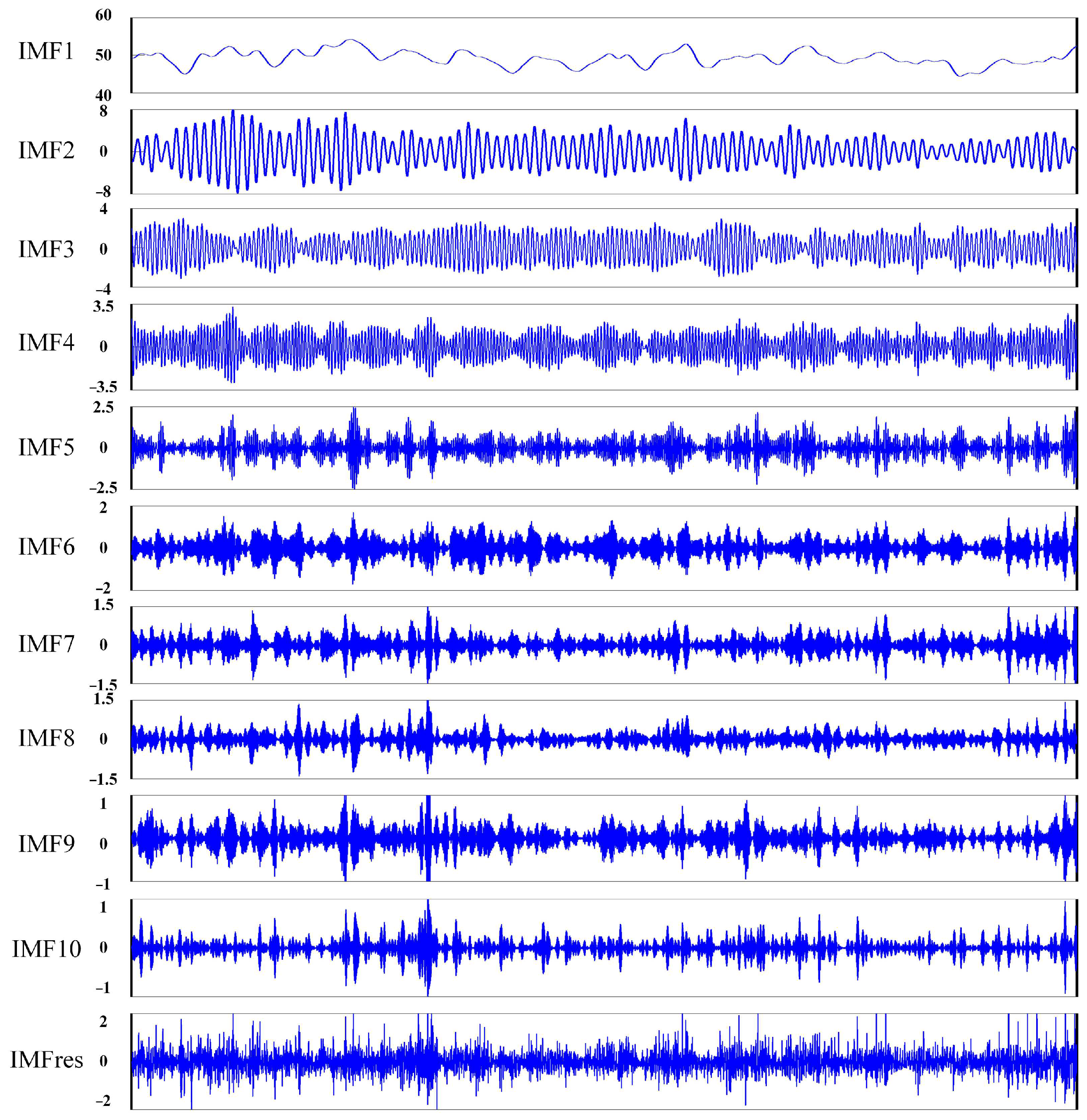
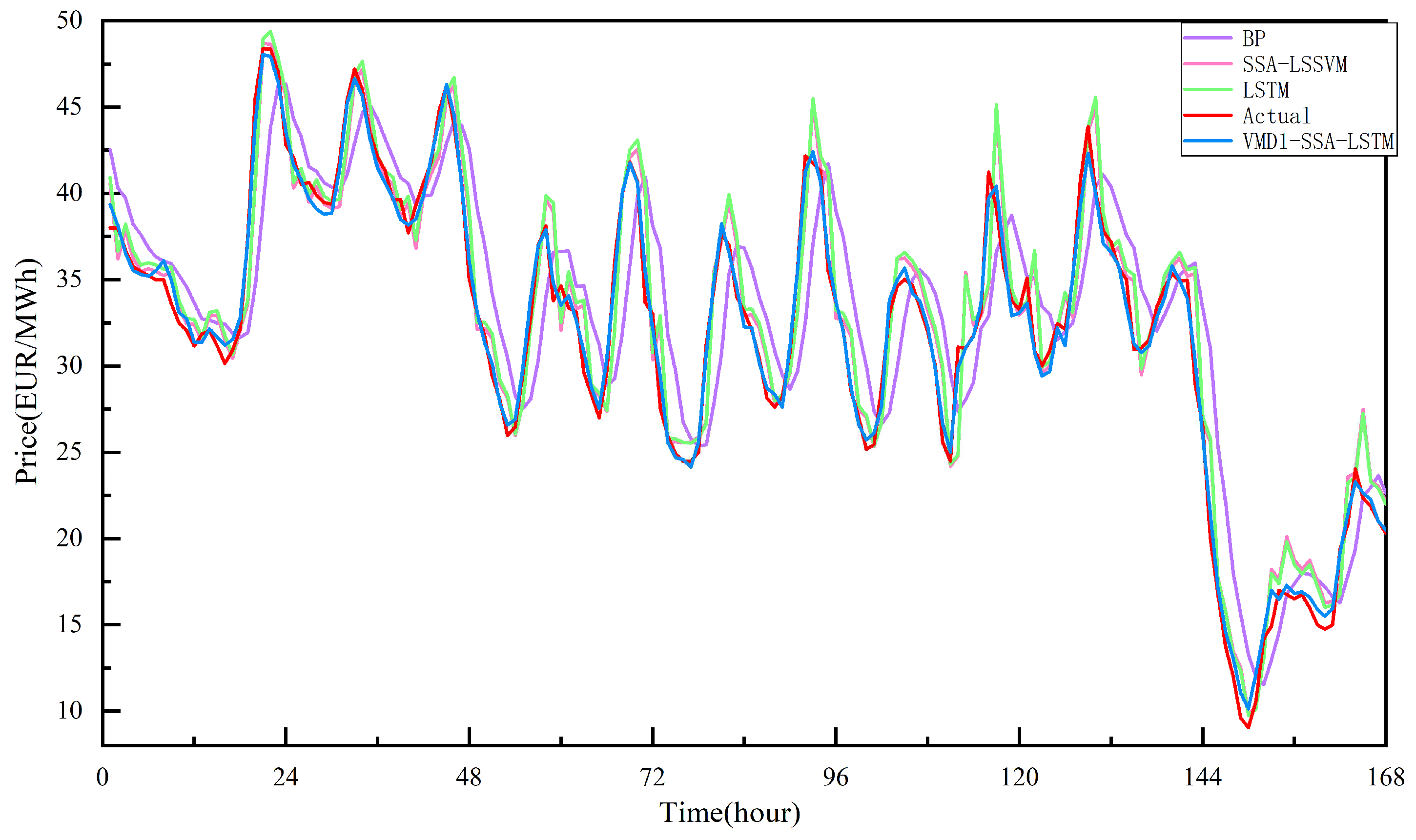
The electricity market in South Wales, Australia, often exhibits high volatility due to frequent external shocks to its electricity prices. In this case, electricity price data for 100 days between 21 January and 30 April 2014, for the New South Wales continent of Australia, were used. As shown in Figure 3, there are 4800 observations, and the original electricity price series has a large variation of ups and downs. Figure 4 illustrates the modal components of several different center frequencies obtained from the original electricity price series after VMD decomposition. After VMD decomposition, the original tariff series’ fluctuating trends and complex internal fluctuation characteristics are assigned to different components. In this way, the SSA-optimized LSTM model can more easily identify and extract the features of all members, thus improving the prediction effect. To further enhance the prediction accuracy, the IMF-worst component with the worst prediction accuracy in the first decomposition is decomposed for the second time using VMD, and the decomposition results are shown in Figure 5. After another corruption, the information implied in IMF-worst can be further extracted, improving the model’s overall prediction.
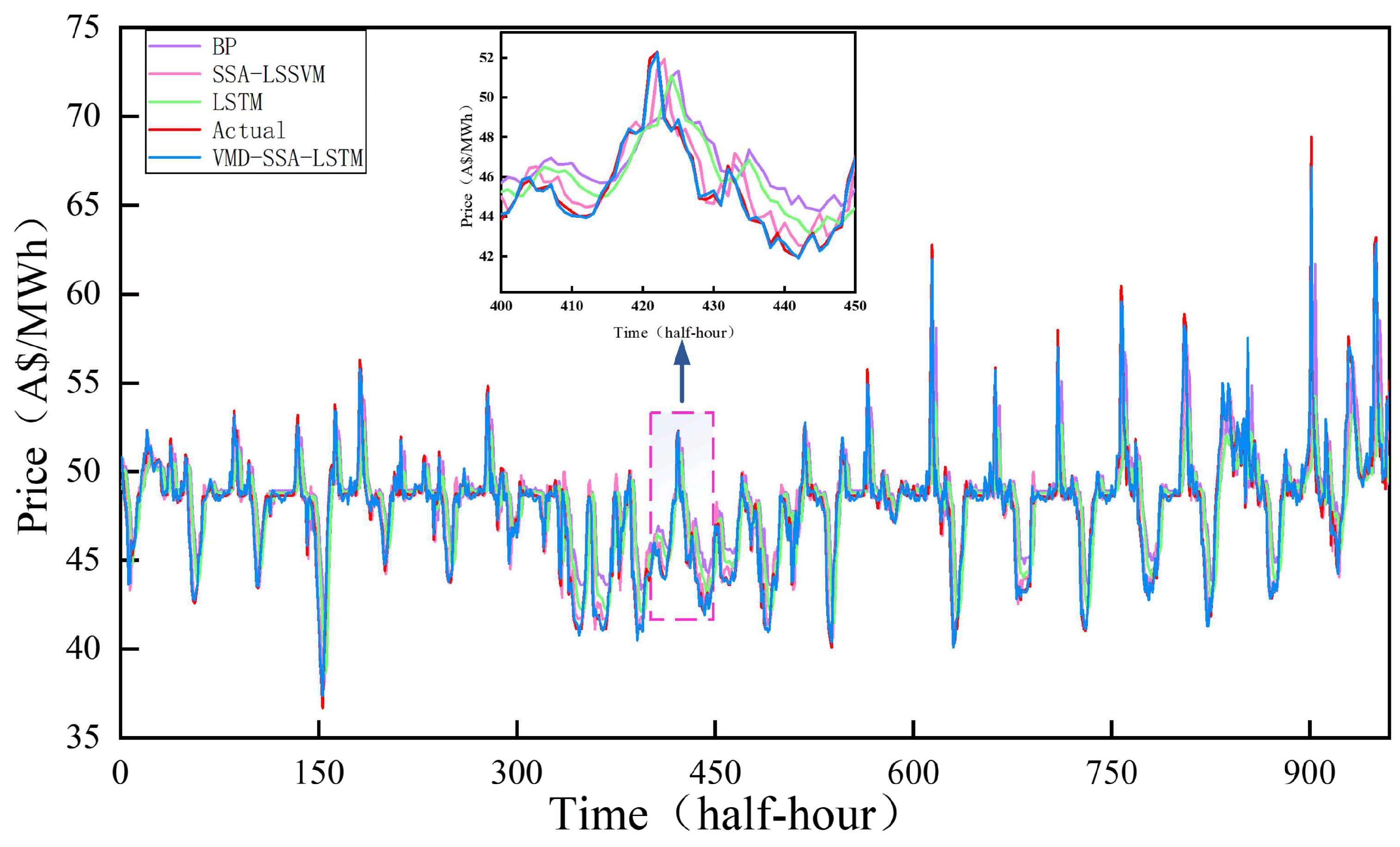
The prediction results of the different models are shown in Figure 6. It can be seen from the figure that the prediction zone curve of the proposed model is very similar to the actual value curve. To further check the prediction accuracy of the models, MAPE, RMSE, and MAE were used to evaluate the models’ prediction errors. Table 1 shows the prediction error metrics of different models, where the proposed model has a MAPE of 0.44%, RMSE of 0.28 (AUD/MWh), and MAE of 0.21 (AUD/MWh). The proposed model significantly improved prediction accuracy compared with BP, LSTM, and SSALSVM models. In addition, the prediction error metrics of single-layer VMD and two-layer VMD are compared in Table 1. The MAPE, RMSE, and MAE are reduced by 0.19%, 0.15 (AUD/MWh), and 0.1 (AUD/MWh) when using two-layer VMD compared with single-layer VMD, indicating that the two-layer VMD decomposition technique can further extract the implied clutter information from the electricity price series to improve the overall prediction effect of the model. And the electricity price series can also perform very well in the face of high electricity price volatility.

4.4. The Case of the French Electricity Market

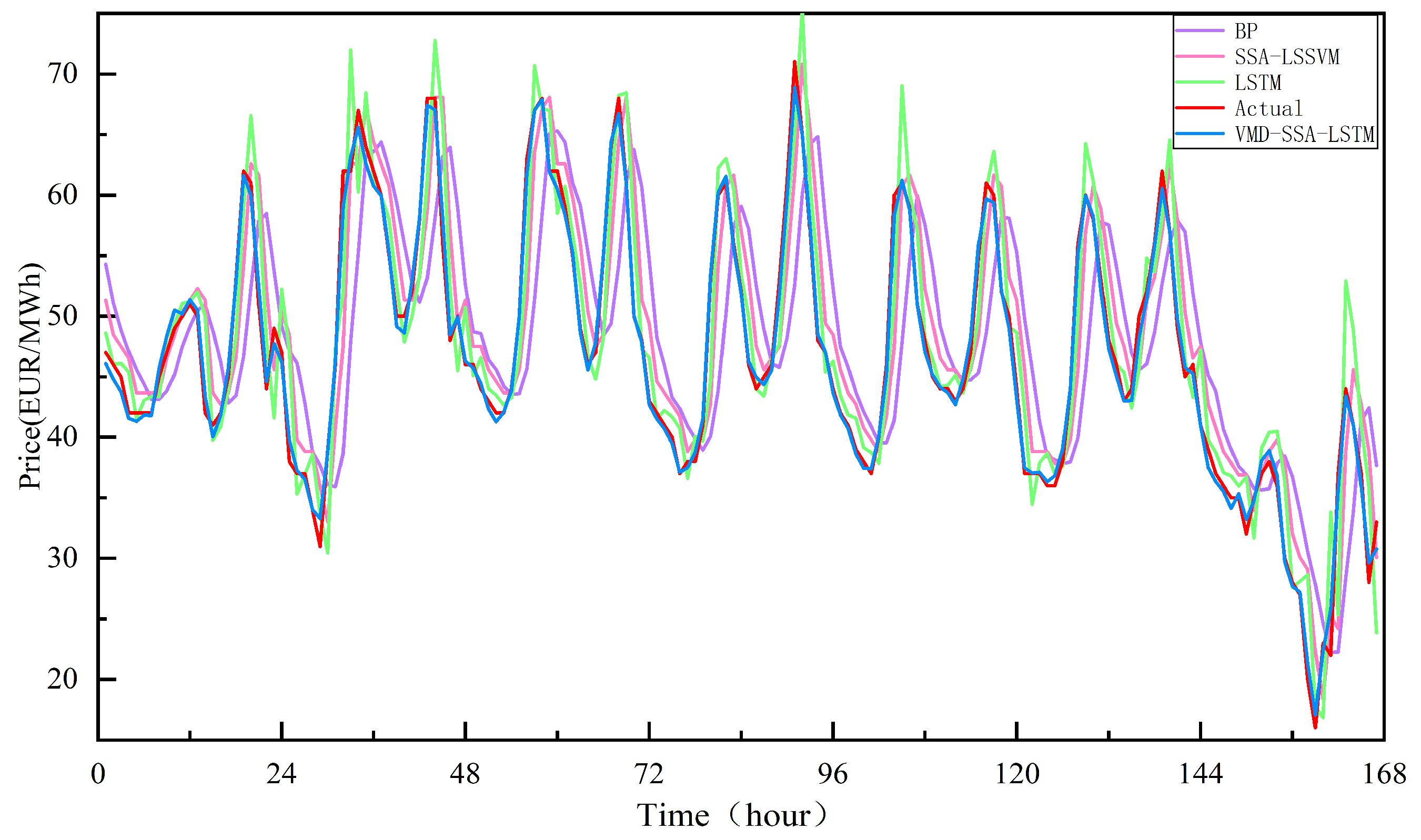
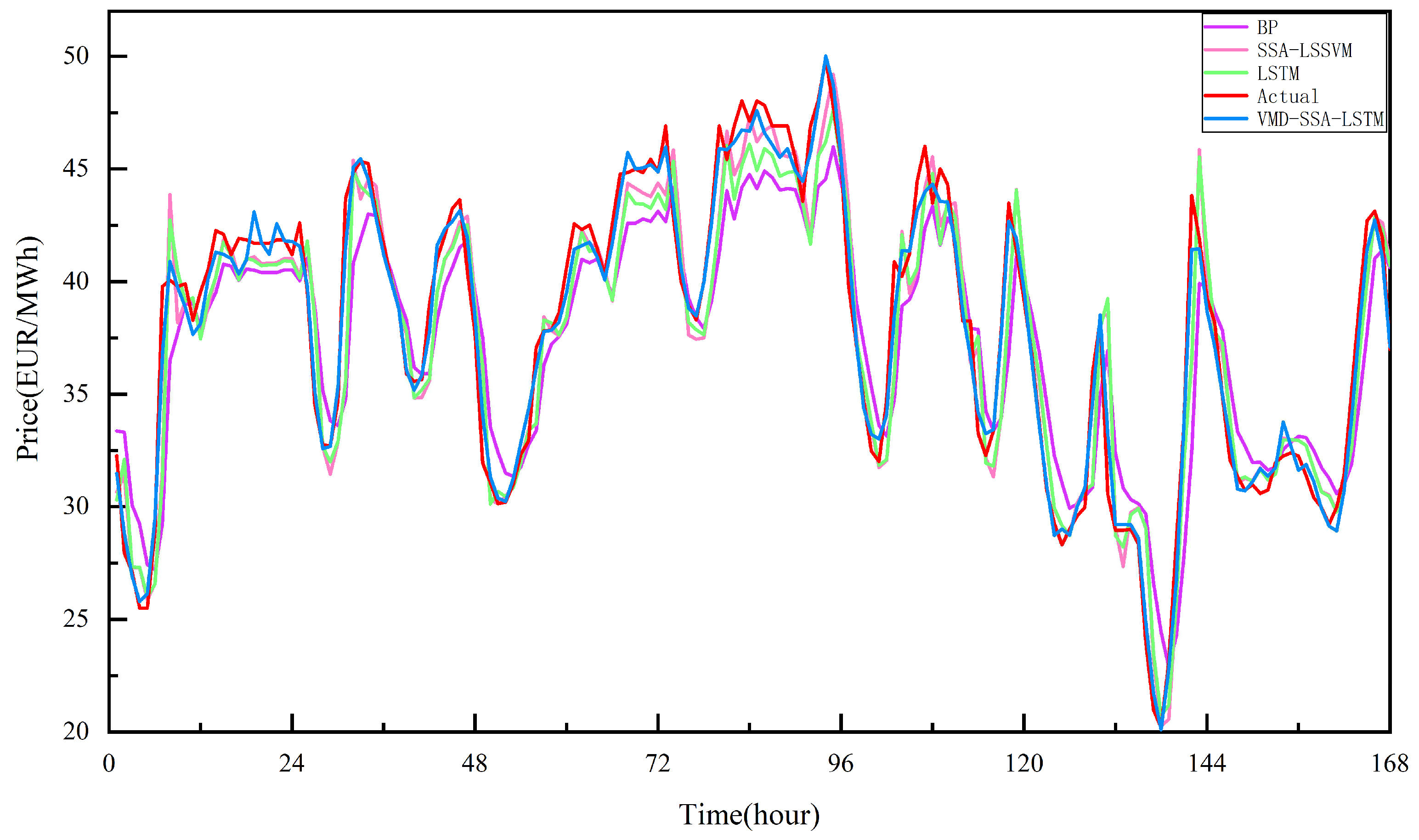
Electricity prices in the French electricity market are relatively stable, with the daily trend being more or less the same. Six weeks of data from 9 January to 20 February 2021, are used in this case. The first five weeks are used as the training set, and the last week with 168 observations, is used as the test set. VMD and input decomposed the original electricity price series to the LSTM model optimized by SSA for training after Min-max normalization. The prediction results are shown in Figure 7. It can be seen from the figure that the predicted values of the proposed model can fit the actual values well and capture the trend and complex features of electricity prices. Figure 8, as well as Table 2, show the prediction error metrics of different models, and it can be seen in the figure that compared to BP, LSTM, and SSA-LSSVM, the proposed model has the smallest MAPE, RMSE, and MAE, indicating that the proposed model has excellent prediction accuracy. In addition, compared with the single-layer VMD, the MAPE, RMSE, and MAE of the proposed two-layer VMD decomposition model in this paper are reduced by 1.54%, 0.8 (EUR/MWh), and 0.67 (EUR/MWh), respectively, indicating that the two-layer VMD decomposition technique can further improve the decomposition effect to reduce the prediction error of the model.

4.5. The Case of the Spanish Electricity Market

The Spanish electricity market has a significant seasonal variation, so in this case, we take this factor into account. In this case, electricity price data are used between 22 December 2019 and 29 November 2020. The data are divided into four different seasons for separate experiments. The data sets span from 22 December 2019 to 29 March 2020 for winter, 23 March to 31 May 2020 for spring, 22 June to 30 August 2020 for summer, and 21 September to 29 November 2020 for fall. Ten weeks of data are used for all four seasons, for 1680 observations. The first nine weeks are used as the training set, and the 168 observations from the last week are used as the test set.
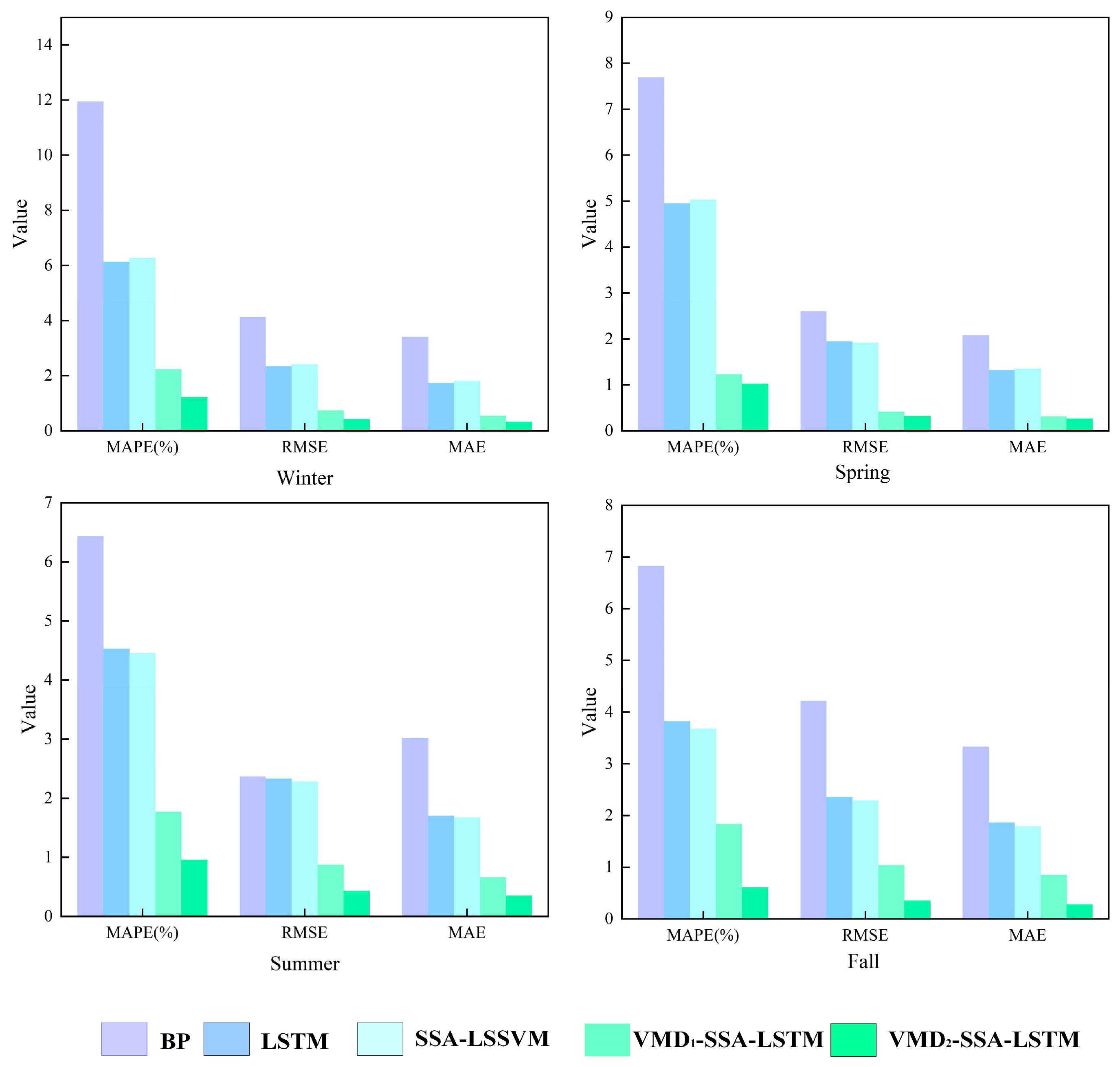
Figure 9, Figure 10, Figure 11 and Figure 12 show the prediction curves of the different models for each of the four seasons. The figures show that the proposed models are very close to the actual electricity price curves, indicating that the proposed models can capture the overall trend of electricity prices well and perform well when there are spikes in electricity prices. The proposed model has very good outstanding forecasting accuracy both in the relatively smooth autumn and in the winter and spring when electricity prices fluctuate greatly. Although there are individual details in the summer curve with more significant errors in the tip electricity price prediction, its overall prediction is still excellent. To further verify the accuracy and stability of the proposed model, MAPE, RMSE, and MAE were calculated for each test week, as shown in Figure 13 and Table 3. By comparing with BP, SSA-LSSVM, and LSTM, we found that the prediction error of the proposed model was significantly reduced in the four seasons. The average MAPE for the four seasons is 0.95%, the average RMSE is 0.38 (EUR/MWh), and the average MAE is 0.31 (EUR/MWh). In addition, the two-layer VMD has better prediction results than the single-layer VMD. The average MAPE is reduced by 0.82%, RMSE by 0.39 (EUR/MWh), and MAE by 0.3 (EUR/MWh) in four seasons, indicating that the two-layer VMD decomposition technique in this paper can further improve the overall prediction accuracy of the model and can adapt well to the changes of the input samples.
In order to further validate the differences in prediction performance between the proposed model and the comparison model and to ensure that the accurate prediction results are stable, the statistical significance of the results needs to be established. We performed Diebold and Mariano (DM) tests [56] on the prediction results of all models based on each of the above cases. The DM test is a statistical test. Table 4 shows the p-values of the DM test results. The null hypothesis is that there is no difference in the prediction accuracy of the models in the rows and columns. The alternative hypothesis is that the model’s prediction accuracy in the column is significantly better than the model in the row. The p-value < 0.01 in Table 4 indicates that the original hypothesis is not valid and the prediction accuracy of the model in the column is significantly better than that of the model in the row. Therefore, we can see that the model’s prediction accuracy incorporating the two-layer VMD decomposition technique is significantly better than several other models.

5. Discussion and Conclusions

EPF is a challenging task, and accurate EPF can provide an essential basis for market participants to develop strategies to reduce risks or maximize benefits in their market transactions. Considering that data for many variables are often difficult to obtain in practical engineering, this study attempts to investigate a prediction method that improves prediction accuracy in scenarios where other variables are not considered, in view of the nonlinear, non-stationarity, and highly volatile characteristics of electricity prices. This paper proposes a hybrid forecasting model consisting of a two-layer VMD decomposition technique and an SSA-optimized LSTM. The model combines the advantages of VMD in terms of data decomposition and LSTM in processing time series. VMD allows decomposing the original electricity price series into multiple modal components with different center frequencies and avoids modal confounding. Optimizing the hyperparameters of the LSTM using SSA can further improve its ability to handle time series. In addition, applying the two-layer VMD to IMF-worst can further extract the complex features implied by the electricity price series to improve the model’s prediction performance. Finally, to test the prediction performance and generalization ability of the model, this paper conducts experimental validation with electricity price data from three electricity markets in New South Wales, Australia, France, and Spain. In addition, the experiments are divided into seasons in the Spanish market. In the case of the New South Wales electricity market, where electricity prices are volatile, we find that the proposed model performs very well, capturing the trend of electricity prices accurately and performing well in the prediction of electricity price spikes despite the large fluctuations in electricity prices. In the case of Spain, we conducted a seasonal forecasting experiment incorporating the seasonal variation in this market. The overall forecasting accuracy is satisfactory, although there are individual cases of large errors in the tip tariffs in the summer forecast result curves. The overall results show that, compared with other models, the proposed model can not only handle the complex features contained in the electricity price series well, but also adapt to the changes of the input samples, and has a better prediction effect and stability. In addition, the proposed two-layer VMD decomposition technique can further deal with the nonlinearity and non-smoothness of the electricity price series and significantly improve the model’s prediction accuracy. This indicates that the proposed model can accurately predict stochastic and non-stationarity electricity price series and can provide key assistance to market participants.
On the other hand, more influencing factors can be considered in future work to further improve the overall forecasting effect and model robustness. Especially with treating spike prices, multi-factor consideration combined with multimodal decomposition may achieve more significant forecasting results. Therefore, in future works, we suggest collecting more real-time data of other variables such as weather, load, and fuel price to facilitate researchers to get better prediction results.

Author Contributions

Conceptualization, F.G. and W.Z.; methodology, F.G.; software, W.Z.; validation, S.D., F.G. and W.Z.; formal analysis, S.D.; investigation, S.D.; resources, A.W. and J.D.; data curation, G.H. and R.W.; writing—original draft preparation, F.G.; writing—review and editing, W.Z., A.W. and J.D.; visualization, S.D.; supervision, A.W. and J.D.; project administration, F.G.; funding acquisition, F.G. All authors have read and agreed to the published version of the manuscript.

Funding

This research was funded by the General University Innovation Team Project of Guangdong, Grant number 2021KCXTD027.

Data Availability Statement

The datasets for this study can be found in the https://www.aemo.com.au, accessed on 16 July 2022 (Australian Energy Market Operator), https://www.nordpoolgroup.com/en/, accessed on 15 July 2022 (NORD POOL), https://www.omie.es/en, accessed on 28 July 2022 (OMIE).

Conflicts of Interest

The authors declare that the research was conducted in the absence of any commercial or financial relationships that could be construed as a potential conflict of interest. The funders had no role in the design of the study; in the collection, analyses, or interpretation of data; in the writing of the manuscript; or in the decision to publish the results.

References

  1. Zugno, M.; Morales, J.M.; Pinson, P.; Madsen, H. A Bilevel Model for Electricity Retailers’ Participation in a Demand Response Market Environment. Energy Econ. 2013, 36, 182–197. [Google Scholar] [CrossRef]
  2. Singh, N.; Mohanty, S.R.; Dev Shukla, R. Short Term Electricity Price Forecast Based on Environmentally Adapted Generalized Neuron. Energy 2017, 125, 127–139. [Google Scholar] [CrossRef]
  3. Lago, J.; De Ridder, F.; Vrancx, P.; De Schutter, B. Forecasting Day-Ahead Electricity Prices in Europe: The Importance of Considering Market Integration. Appl. Energy 2018, 211, 890–903. [Google Scholar] [CrossRef]
  4. Shah, I.; Bibi, H.; Ali, S.; Wang, L.; Yue, Z. Forecasting One-Day-Ahead Electricity Prices for Italian Electricity Market Using Parametric and Nonparametric Approaches. IEEE Access 2020, 8, 123104–123113. [Google Scholar] [CrossRef]
  5. Shao, Z.; Zheng, Q.; Liu, C.; Gao, S.; Wang, G.; Chu, Y. A Feature Extraction- and Ranking-Based Framework for Electricity Spot Price Forecasting Using a Hybrid Deep Neural Network. Electr. Power Syst. Res. 2021, 200, 107453. [Google Scholar] [CrossRef]
  6. Shah, I.; Akbar, S.; Saba, T.; Ali, S.; Rehman, A. Short-Term Forecasting for the Electricity Spot Prices With Extreme Values Treatment. IEEE Access 2021, 9, 105451–105462. [Google Scholar] [CrossRef]
  7. Li, W.; Becker, D.M. Day-Ahead Electricity Price Prediction Applying Hybrid Models of LSTM-Based Deep Learning Methods and Feature Selection Algorithms under Consideration of Market Coupling. Energy 2021, 237, 121543. [Google Scholar] [CrossRef]
  8. Shah, I.; Iftikhar, H.; Ali, S.; Wang, D. Short-Term Electricity Demand Forecasting Using Components Estimation Technique. Energies 2019, 12, 2532. [Google Scholar] [CrossRef] [Green Version]
  9. Lago, J.; Marcjasz, G.; De Schutter, B.; Weron, R. Forecasting Day-Ahead Electricity Prices: A Review of State-of-the-Art Algorithms, Best Practices and an Open-Access Benchmark. Appl. Energy 2021, 293, 116983. [Google Scholar] [CrossRef]
  10. Narajewski, M.; Ziel, F. Econometric Modelling and Forecasting of Intraday Electricity Prices. J. Commod. Mark. 2020, 19, 100107. [Google Scholar] [CrossRef]
  11. Girish, G.P. Spot Electricity Price Forecasting in Indian Electricity Market Using Autoregressive-GARCH Models. Energy Strategy Rev. 2016, 11–12, 52–57. [Google Scholar] [CrossRef]
  12. Liu, H.; Shi, J. Applying ARMA–GARCH Approaches to Forecasting Short-Term Electricity Prices. Energy Econ. 2013, 37, 152–166. [Google Scholar] [CrossRef]
  13. Chang, Z.; Zhang, Y.; Chen, W. Electricity Price Prediction Based on Hybrid Model of Adam Optimized LSTM Neural Network and Wavelet Transform. Energy 2019, 187, 115804. [Google Scholar] [CrossRef]
  14. Tan, Z.; Zhang, J.; Wang, J.; Xu, J. Day-Ahead Electricity Price Forecasting Using Wavelet Transform Combined with ARIMA and GARCH Models. Appl. Energy 2010, 87, 3606–3610. [Google Scholar] [CrossRef]
  15. Yang, Z.; Ce, L.; Lian, L. Electricity Price Forecasting by a Hybrid Model, Combining Wavelet Transform, ARMA and Kernel-Based Extreme Learning Machine Methods. Appl. Energy 2017, 190, 291–305. [Google Scholar] [CrossRef]
  16. Zhang, J.-L.; Zhang, Y.-J.; Li, D.-Z.; Tan, Z.-F.; Ji, J.-F. Forecasting Day-Ahead Electricity Prices Using a New Integrated Model. Int. J. Electr. Power Energy Syst. 2019, 105, 541–548. [Google Scholar] [CrossRef]
  17. Panapakidis, I.P.; Dagoumas, A.S. Day-Ahead Electricity Price Forecasting via the Application of Artificial Neural Network Based Models. Appl. Energy 2016, 172, 132–151. [Google Scholar] [CrossRef]
  18. Mosbah, H.; El-hawary, M. Hourly Electricity Price Forecasting for the Next Month Using Multilayer Neural Network. Can. J. Electr. Comput. Eng. 2016, 39, 283–291. [Google Scholar] [CrossRef]
  19. Keles, D.; Scelle, J.; Paraschiv, F.; Fichtner, W. Extended Forecast Methods for Day-Ahead Electricity Spot Prices Applying Artificial Neural Networks. Appl. Energy 2016, 162, 218–230. [Google Scholar] [CrossRef]
  20. Zhang, C.; Li, R.; Shi, H.; Li, F. Deep Learning for Day-Ahead Electricity Price Forecasting. IET Smart Grid 2020, 3, 462–469. [Google Scholar] [CrossRef]
  21. Shiri, A.; Afshar, M.; Rahimi-Kian, A.; Maham, B. Electricity Price Forecasting Using Support Vector Machines by Considering Oil and Natural Gas Price Impacts. In Proceedings of the 2015 IEEE International Conference on Smart Energy Grid Engineering, Oshawa, ON, Canada, 17–19 August 2015; pp. 1–5. [Google Scholar]
  22. Che, J.; Wang, J. Short-Term Electricity Prices Forecasting Based on Support Vector Regression and Auto-Regressive Integrated Moving Average Modeling. Energy Convers. Manag. 2010, 51, 1911–1917. [Google Scholar] [CrossRef]
  23. Imani, M.H.; Bompard, E.; Colella, P.; Huang, T. Forecasting Electricity Price in Different Time Horizons: An Application to the Italian Electricity Market. IEEE Trans. Ind. Appl. 2021, 57, 5726–5736. [Google Scholar] [CrossRef]
  24. Najafi, A.; Homaee, O.; Jasinski, M.; Golshan, M.; Leonowicz, Z. Application of Extreme Learning Machine-Autoencoder to Medium Term Electricity Price Forecasting. In Proceedings of the 2022 IEEE International Conference on Environment and Electrical Engineering and 2022 IEEE Industrial and Commercial Power Systems Europe, Prague, Czech Republic, 28 June–1 July 2022; pp. 1–4. [Google Scholar]
  25. Wang, L.; Zhang, Z.; Chen, J. Short-Term Electricity Price Forecasting With Stacked Denoising Autoencoders. IEEE Trans. Power Syst. 2017, 32, 2673–2681. [Google Scholar] [CrossRef]
  26. Wang, D.; Luo, H.; Grunder, O.; Lin, Y.; Guo, H. Multi-Step Ahead Electricity Price Forecasting Using a Hybrid Model Based on Two-Layer Decomposition Technique and BP Neural Network Optimized by Firefly Algorithm. Appl. Energy 2017, 190, 390–407. [Google Scholar] [CrossRef]
  27. Yi, M.; Xie, W.; Mo, L. Short-Term Electricity Price Forecasting Based on BP Neural Network Optimized by SAPSO. Energies 2021, 14, 6514. [Google Scholar] [CrossRef]
  28. Anbazhagan, S.; Kumarappan, N. Day-Ahead Deregulated Electricity Market Price Forecasting Using Recurrent Neural Network. IEEE Syst. J. 2013, 7, 866–872. [Google Scholar] [CrossRef]
  29. Khan, Z.A.; Fareed, S.; Anwar, M.; Naeem, A.; Gul, H.; Arif, A.; Javaid, N. Short Term Electricity Price Forecasting Through Convolutional Neural Network (CNN). In Proceedings of the Web, Artificial Intelligence and Network Applications, Caserta, Italy, 15–17 April 2020; Springer: Cham, Switzerland, 2020; pp. 1181–1188. [Google Scholar]
  30. Abedinia, O.; Amjady, N.; Shafie-khah, M.; Catalão, J.P.S. Electricity Price Forecast Using Combinatorial Neural Network Trained by a New Stochastic Search Method. Energy Convers. Manag. 2015, 105, 642–654. [Google Scholar] [CrossRef]
  31. Yang, Y.; Tan, Z.; Yang, H.; Ruan, G.; Zhong, H.; Liu, F. Short-Term Electricity Price Forecasting Based on Graph Convolution Network and Attention Mechanism. IET Renew. Power Gener. 2022, 16, 2481–2492. [Google Scholar] [CrossRef]
  32. Afrasiabi, M.; Mohammadi, M.; Rastegar, M.; Kargarian, A. Probabilistic Deep Neural Network Price Forecasting Based on Residential Load and Wind Speed Predictions. IET Renew. Power Gener. 2019, 13, 1840–1848. [Google Scholar] [CrossRef]
  33. Peng, L.; Liu, S.; Liu, R.; Wang, L. Effective Long Short-Term Memory with Differential Evolution Algorithm for Electricity Price Prediction. Energy 2018, 162, 1301–1314. [Google Scholar] [CrossRef]
  34. Gundu, V.; Simon, S.P. PSO–LSTM for Short Term Forecast of Heterogeneous Time Series Electricity Price Signals. J. Ambient. Intell. Hum. Comput 2021, 12, 2375–2385. [Google Scholar] [CrossRef]
  35. Lahmiri, S. Comparing Variational and Empirical Mode Decomposition in Forecasting Day-Ahead Energy Prices. IEEE Syst. J. 2017, 11, 1907–1910. [Google Scholar] [CrossRef]
  36. Naz, A.; Javed, M.U.; Javaid, N.; Saba, T.; Alhussein, M.; Aurangzeb, K. Short-Term Electric Load and Price Forecasting Using Enhanced Extreme Learning Machine Optimization in Smart Grids. Energies 2019, 12, 866. [Google Scholar] [CrossRef] [Green Version]
  37. Gholipour Khajeh, M.; Maleki, A.; Rosen, M.A.; Ahmadi, M.H. Electricity Price Forecasting Using Neural Networks with an Improved Iterative Training Algorithm. Int. J. Ambient Energy 2018, 39, 147–158. [Google Scholar] [CrossRef]
  38. Victoire, T.A.A.; Gobu, B.; Jaikumar, S.; Arulmozhi, N.; Kanimozhi, P.; Victoire, T.A. Two-Stage Machine Learning Framework for Simultaneous Forecasting of Price-Load in the Smart Grid. In Proceedings of the 2018 17th IEEE International Conference on Machine Learning and Applications, Orlando, FL, USA, 17–20 December 2018; pp. 1081–1086. [Google Scholar]
  39. Darudi, A.; Bashari, M.; Javidi, M.H. Electricity Price Forecasting Using a New Data Fusion Algorithm. IET Gener. Transm. Distrib. 2015, 9, 1382–1390. [Google Scholar] [CrossRef]
  40. Gao, W.; Darvishan, A.; Toghani, M.; Mohammadi, M.; Abedinia, O.; Ghadimi, N. Different States of Multi-Block Based Forecast Engine for Price and Load Prediction. Int. J. Electr. Power Energy Syst. 2019, 104, 423–435. [Google Scholar] [CrossRef]
  41. Pourdaryaei, A.; Mokhlis, H.; Illias, H.A.; Kaboli, S.H.A.; Ahmad, S. Short-Term Electricity Price Forecasting via Hybrid Backtracking Search Algorithm and ANFIS Approach. IEEE Access 2019, 7, 77674–77691. [Google Scholar] [CrossRef]
  42. Yang, W.; Sun, S.; Hao, Y.; Wang, S. A Novel Machine Learning-Based Electricity Price Forecasting Model Based on Optimal Model Selection Strategy. Energy 2022, 238, 121989. [Google Scholar] [CrossRef]
  43. Zhang, F.; Fleyeh, H.; Bales, C. A Hybrid Model Based on Bidirectional Long Short-Term Memory Neural Network and Catboost for Short-Term Electricity Spot Price Forecasting. J. Oper. Res. Soc. 2022, 73, 301–325. [Google Scholar] [CrossRef]
  44. Chen, Y.; Li, M.; Yang, Y.; Li, C.; Li, Y.; Li, L. A Hybrid Model for Electricity Price Forecasting Based on Least Square Support Vector Machines with Combined Kernel. J. Renew. Sustain. Energy 2018, 10, 055502. [Google Scholar] [CrossRef]
  45. Hong, Y.-Y.; Liu, C.-Y.; Chen, S.-J.; Huang, W.-C.; Yu, T.-H. Short-Term LMP Forecasting Using an Artificial Neural Network Incorporating Empirical Mode Decomposition. Int. Trans. Electr. Energy Syst. 2015, 25, 1952–1964. [Google Scholar] [CrossRef]
  46. He, K.; Yu, L.; Tang, L. Electricity Price Forecasting with a BED (Bivariate EMD Denoising) Methodology. Energy 2015, 91, 601–609. [Google Scholar] [CrossRef]
  47. Qiu, X.; Suganthan, P.N.; Amaratunga, G.A.J. Short-Term Electricity Price Forecasting with Empirical Mode Decomposition Based Ensemble Kernel Machines. Procedia Comput. Sci. 2017, 108, 1308–1317. [Google Scholar] [CrossRef]
  48. Zhang, J.; Tan, Z.; Wei, Y. An Adaptive Hybrid Model for Short Term Electricity Price Forecasting. Appl. Energy 2020, 258, 114087. [Google Scholar] [CrossRef]
  49. Jiang, P.; Ma, X. A Hybrid Forecasting Approach Applied in the Electrical Power System Based on Data Preprocessing, Optimization and Artificial Intelligence Algorithms. Appl. Math. Model. 2016, 40, 10631–10649. [Google Scholar] [CrossRef]
  50. Huang, C.-J.; Shen, Y.; Chen, Y.-H.; Chen, H.-C. A Novel Hybrid Deep Neural Network Model for Short-Term Electricity Price Forecasting. Int. J. Energy Res. 2021, 45, 2511–2532. [Google Scholar] [CrossRef]
  51. Zhang, T.; Tang, Z.; Wu, J.; Du, X.; Chen, K. Short Term Electricity Price Forecasting Using a New Hybrid Model Based on Two-Layer Decomposition Technique and Ensemble Learning. Electr. Power Syst. Res. 2022, 205, 107762. [Google Scholar] [CrossRef]
  52. Heydari, A.; Majidi Nezhad, M.; Pirshayan, E.; Astiaso Garcia, D.; Keynia, F.; De Santoli, L. Short-Term Electricity Price and Load Forecasting in Isolated Power Grids Based on Composite Neural Network and Gravitational Search Optimization Algorithm. Appl. Energy 2020, 277, 115503. [Google Scholar] [CrossRef]
  53. Dragomiretskiy, K.; Zosso, D. Variational Mode Decomposition. IEEE Trans. Signal Process. 2014, 62, 531–544. [Google Scholar] [CrossRef]
  54. Xue, J.; Shen, B. A Novel Swarm Intelligence Optimization Approach: Sparrow Search Algorithm. Syst. Sci. Control Eng. 2020, 8, 22–34. [Google Scholar] [CrossRef]
  55. Hochreiter, S.; Schmidhuber, J. Long Short-Term Memory. Neural Comput. 1997, 9, 1735–1780. [Google Scholar] [CrossRef] [PubMed]
  56. Diebold, F.X.; Mariano, R.S. Comparing Predictive Accuracy. J. Bus. Econ. Stat. 2002, 20, 134–144. [Google Scholar] [CrossRef]
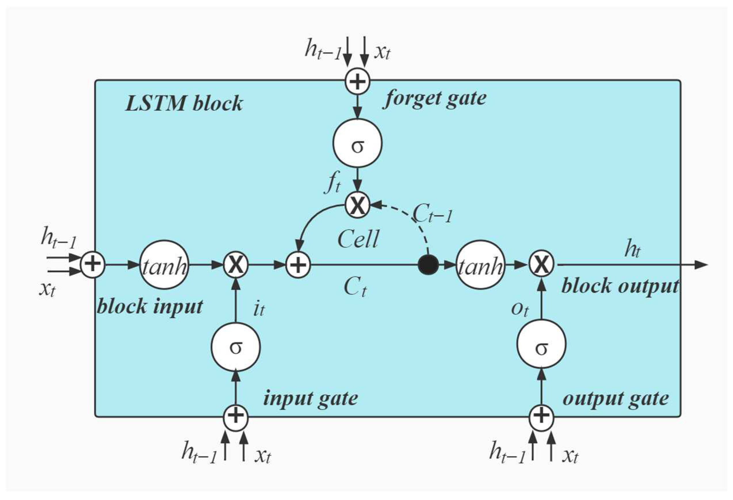
Figure 1. Schematic diagram of LSTM cell structure.
Energies 15 08445 g001
Figure 2. Block diagram of the prediction process of the VMD-SSA-LSTM model.
Energies 15 08445 g002
Figure 3. Original electricity price series.
Energies 15 08445 g003
Figure 4. Decomposition results of the first variational modal decomposition.
Energies 15 08445 g004
Figure 5. Decomposition results of IMF-worst.
Energies 15 08445 g005
Figure 6. NSW prediction result curve.
Energies 15 08445 g006
Figure 7. France prediction result curve.
Energies 15 08445 g007
Figure 8. France forecast error indicators.
Energies 15 08445 g008
Figure 9. Curve of winter forecast results for Spain.
Energies 15 08445 g009
Figure 10. Curve of spring forecast results for Spain.
Energies 15 08445 g010
Figure 11. Curve of summer forecast results for Spain.
Energies 15 08445 g011
Figure 12. Curve of fall forecast results for Spain.
Energies 15 08445 g012
Figure 13. Spanish forecast error indicators.
Energies 15 08445 g013
Table 1. Error metrics for different prediction models in NSW.
BPLSTMSSA-LSSVMVMD1-SSA-LSTMVMD2-SSA-LSTM
MAPE (%)3.672.411.910.630.39
RMSE2.541.841.580.430.25
MAE1.741.170.940.310.19
VMD1 is single-layer VMD. VMD2 is tow-layer VMD.
Table 2. Error metrics for different prediction models in French.
BPLSTMSSA-LSSVMVMD1-SSA-LSTMVMD2-SSA-LSTM
MAPE (%)15.49.898.083.121.58
RMSE8.395.344.511.700.90
MAE6.994.323.481.350.68
VMD1 is single-layer VMD. VMD2 is tow-layer VMD.
Table 3. Error metrics for different prediction models in Spain.
SeasonError MetricsModel
BPSSA-LSSVMLSTMVMD1-SSA-LSTMVMD2-SSA-LSTM
WinterMAPE (%)11.946.136.282.231.22
RMSE4.132.342.410.740.42
MAE3.411.741.810.610.33
SpringMAPE (%)7.695.034.951.231.02
RMSE2.601.921.950.420.32
MAE2.081.351.320.310.26
SummerMAPE (%)6.434.464.531.770.96
RMSE2.372.282.330.870.43
MAE3.021.671.700.670.35
FallMAPE (%)6.833.683.831.830.61
RMSE4.222.292.361.040.35
MAE3.331.791.860.850.28
AverageMAPE (%)8.22 4.83 4.90 1.770.95
RMSE3.33 2.21 2.26 0.770.38
MAE2.96 1.64 1.67 0.61 0.31
VMD1 is single-layer VMD. VMD2 is tow-layer VMD.
Table 4. p-values of the Diebold and Mariano test.
MarketModelsBPLSTMSSA-LSSVMVMD1VMD2
AustraliaBP<0.01<0.01<0.01<0.01
LSTM0.99<0.01<0.01<0.01
SSA-LSSVM0.990.99<0.01<0.01
VMD10.990.990.99<0.01
VMD20.990.990.990.99
FranceBP<0.01<0.01<0.01<0.01
LSTM0.99<0.01<0.01<0.01
SSA-LSSVM0.990.99<0.01<0.01
VMD10.990.990.99<0.01
VMD20.990.990.990.99
Spain—SpringBP<0.01<0.01<0.01<0.01
LSTM0.99<0.01<0.01<0.01
SSA-LSSVM0.990.99<0.01<0.01
VMD10.990.990.99<0.01
VMD20.990.990.990.99
Spain—SummerBP<0.01<0.01<0.01<0.01
LSTM0.990.05<0.01<0.01
SSA-LSSVM0.990.95<0.01<0.01
VMD10.990.990.99<0.01
VMD20.990.990.990.99
Spain—FallBP<0.01<0.01<0.01<0.01
LSTM0.990.02<0.01<0.01
SSA-LSSVM0.990.98<0.01<0.01
VMD10.990.990.99<0.01
VMD20.990.990.990.99
Spain—WinterBP<0.01<0.01<0.01<0.01
LSTM0.99<0.01<0.01<0.01
SSA-LSSVM0.990.99<0.01<0.01
VMD10.990.990.99<0.01
VMD20.990.990.990.99
VMD1 is single-layer VMD. VMD2 is tow-layer VMD. Null hypothesis: models in rows and columns have equal prediction accuracy; alternative hypothesis: models in columns are more accurate than models in rows.
Publisher’s Note: MDPI stays neutral with regard to jurisdictional claims in published maps and institutional affiliations.