Sliding-Mode Current Control with Exponential Reaching Law for a Three-Phase Induction Machine Fed by a Direct Matrix Converter

Abstract

The direct matrix converter (DMC) is considered to be an exciting power converter topology option for electric motor drives in industrial applications (elevators, hoists and cranes) and applications where size and weight are critical (e.g., the aerospace industry). Several control techniques have been developed to exploit the DMC’s benefits and achieve the desired performance with classic control techniques, such as field-oriented control and direct torque control, and more sophisticated ones, such as model predictive control and sliding mode control (SMC). SMC is attractive due to its robustness and fast response. However, this control strategy suffers from a phenomenon called chattering. Thus, a solution based on the exponential reaching law (ERL) is implemented to resolve this issue. The proposed method was validated using simulation and experimental results from tests on a three-phase induction machine.

1. Introduction

Power electronic converters are a fundamental part of applications related to using renewable energies (wind, solar) and propulsion of electric or hybrid vehicles [1,2]. The evolution in the development of power electronic semiconductors has led to the implementation of more efficient, more undersized and more lightweight power converters. These before-mentioned aspects are of outstanding significance in the race for power efficiency, electric-based transportation and the integration of renewables. Consequently, a power electronic converter that has become relevant recently is the direct matrix converter (DMC). The DMC is a direct AC–AC electronic power converter, which transforms AC power directly through an array of bidirectional switches, replacing the traditional AC–AC conversion method with rectification stage, intermediate filters and inversion [3,4]. The following advantages of the DMC have been observed compared to the commonly used back-to-back type power converters:

• Reduced volume as a consequence of the lack of large energy-storage capacitors,
• Decreased conduction losses and
• The option of regeneration of energy from the load to supply because of circuits’ natural bi-directionality [5,6,7,8].

Furthermore, the DMC can adjust the output voltages, frequencies and amplitudes according to the requirement of the grid or load. However, these advantages do come at the cost of slightly more semiconductor devices and greater complexity in the development of modulation strategies; and at the time of experimental implementation, it requires considerable computational time, depending on the control strategy to be implemented, so it is crucial to analyse the appropriate digital devices in terms of working bandwidth.

The DMC topology was first proposed in the mid-1970s [9]. At that moment, controllable semiconductor-based power devices were not available. However, in recent decades, industrial and investigation applications of DMCs have risen primarily because of the reduction in the cost of insulated gate bipolar transistor (IGBT) semiconductors, and more recently, silicon carbide-metal-oxide-semiconductor field-effect transistors (SiC-MOSFETs) [10,11,12].

The three-phase induction machine (IM) has been widely used in industry in low-and medium-power applications. Among the advantages that justify its use are its low cost, simple construction, high robustness and ease of maintenance [13]. High-power applications commonly employ multilevel converters, such as neutral point clamping (NPC) [14,15]. For low- and medium-power ones, the topologies named back-to-back (BTB) and voltage source inverter (VSI) are the most popular choices [16,17]. BTB consists of a two-stage AC-DC-AC conversion that employs huge capacitors for the DC link. This also implies a higher volume and higher weight of the power converter. Note that the DC-bus capacitor is an indispensable component of the VSI and accounts for up to two thirds of the volume of the inverter [18]. As an exciting alternative, the DMC can be considered for electric motor drives in industrial applications (elevators, hoists and cranes) and applications where size and weight are critical (e.g., the aerospace industry) [19].

To apply advanced control techniques to IMs, it is necessary to use a power electronic converter, which allows for regulating the frequency and amplitude of the currents or voltages delivered to the machine [20]. The most widely used three-phase IM control techniques in high-performance applications are field-oriented control (FOC) and direct torque control (DTC) [21,22].

Although there is vast experience in using three-phase IMs, the development of precise and robust control strategies continues to be a significant challenge due to their construction characteristics and nature. They are represented by multivariable mathematical models, in which not all variables are measurable and are also related to each other in a nonlinear way. This produces inaccuracies in controlling and estimating variables when using simplified or linearised systems [23]. With the development of higher-power digital signal processors, cutting-edge control approaches have been presented; some instances include finite-control-set model predictive control (FCS-MPC) and the sliding mode control (SMC) [24]. FCS-MPC is one of the IM’s most popular control techniques [25]. FCS-MPC is typically implemented as predictive current control (PCC) or predictive torque control (PTC) in the inner control loop of field-oriented control [26]. Its quick dynamic response and straightforward inclusion of constraints are the main benefits of FCS-MPC [27]. Yet, it suffers from an elevated computational load and highly depends on the system’s accurate model. Recently, SMC has appeared as a promising option due to its robustness, easy tuning of controller parameters, fast dynamic response and lack of a need for high computational power [28]. The following are a few recent works on SMC and its applications [29,30,31]. However, in practice, SMC presents an unwanted phenomenon called chattering, which can be reduced using the exponential reaching law (ERL).

This article presents the DMC as an alternative to feed the three-phase IM and proposes a robust current regulator based on the SMC approach. This innovative system inherits the advantages of both IM machines and the DMC mentioned above. According to the best of the authors knowledge, most of the proposed current control techniques applied to this system fall into deviations of FOC or FCS-MPC. Therefore, the principal contribution of this article focuses on implementing a robust SMC equipped with the ERL. In this context, experimental analyses are presented to validate the proposal and thus contribute to the state-of-the-art of controlling the system mentioned above. The experimental results were obtained by analyzing different conditions, considering stationary and transient operating regimes under different gains of the proposed controller and varying the electrical parameters.

The remainder of the article is organized as follows. Section 2 provides the three-phase IM mathematical model employed for the SMC. Section 3 presents the classical SMC, the sliding surface design and the enhanced SMC, namely, SMC-ERL. The results obtained are given in Section 4 and Section 5—simulation and experimental, respectively. Ultimately, the findings future research works are included in Section 6.

2. System Conversion Description

The DMC is connected to an AC voltage source via an input filter, which is intended to prevent over-voltages and reduce high-frequency elements in the input currents. A single-stage converter with $m\times n$ bidirectional power switches connecting an m phase voltage source to an n phase load constitutes the schematic circuit of the DMC, as shown in Figure 1. Each bidirectional switch is identified with a variable $S_{ij}$, also named the switching function, $iϵ\{u,v,w\}$ being the input and $jϵ\{a,b,c\}$ the output. Note that $S_{ij}$ can take the following values: $S_{ij}=1$ (when the switch $ij$ is conducting, on or closed) or $S_{ij}=0$ (when the switch $ij$ is blocked, off or open). It is important to mention that, in each column, only one switch can be flipped. This is because of the existence of capacitors at the DMC input.

In addition, due to the load’s inductive nature, it is unthinkable to interrupt the current flowing through it suddenly. Consequently, in each column, at least one switch must be activated. The above constraints can be represented mathematically using the following equation: $S_{uj}+S_{vj}+S_{wj}=1,\forall j\in \{a,b,c\}$. Under these constraints, the DMC gives 27 possible switching combinations allowed among the $2^9=512$ total combinations.

2.1. IM Mathematical Model

The following equations represent the mathematical model of the IM in the state-space representation [32]:

$$\begin{array}{cc}\dot{\mathbf{x}}\left(t\right)\hfill & =f(\mathbf{x},t)+g\mathbf{u}\left(t\right),\hfill \\ \mathbf{y}\left(t\right)\hfill & =\mathbf{C}\mathbf{x}\left(t\right),\hfill \end{array}$$

(1)

being the state vector composed of the stator and rotor currents in $(\alpha ,\beta )$ subspace and the rotor speed as follows: $\mathbf{x}\left(t\right)={\left[i_{s\alpha },i_{s\beta },i_{r\alpha },i_{r\beta },{\omega }_r\right]}^T$. In addition, $f(\mathbf{x},t)$, g and $\mathbf{C}$ are given by:

$$f(\mathbf{x},t)=\mathcal{L}\left[\begin{array}{c}{L}_r{R}_s{i}_{s\alpha }-L_m^2{\omega }_r{i}_{s\beta }-L_m{R}_r{i}_{r\alpha }-L_m{L}_r{\omega }_r{i}_{r\beta }\\ L_m^2{\omega }_r{i}_{s\alpha }+L_r{R}_s{i}_{s\beta }+L_m{L}_r{\omega }_r{i}_{r\alpha }-L_m{R}_r{i}_{r\beta }\\ -L_m{R}_s{i}_{s\alpha }+{\omega }_r{L}_m{L}_s{i}_{s\beta }+R_r{L}_s{i}_{r\alpha }+{\omega }_r{L}_r{L}_s{i}_{r\beta }\\ -{\omega }_r{L}_m{L}_s{i}_{s\alpha }-L_m{R}_s{i}_{s\beta }-{\omega }_r{L}_r{L}_s{i}_{r\alpha }+R_r{L}_s{i}_{r\beta }\\ \left(-\frac{B}{J}{\omega }_r+P^2\frac{L_m}{J}(i_{r\alpha }{i}_{s\beta }-i_{r\beta }{i}_{s\alpha })-\frac{P}{J}{T}_L\right)\frac{1}{\mathcal{L}}\end{array}\right],$$

(2)

$$g=\mathcal{L}\left[\begin{array}{cc}-L_r& 0\\ 0& -L_r\\ L_m& 0\\ 0& L_m\\ 0& 0\end{array}\right],$$

(3)

$$\mathcal{L}={(L_m^2-L_s{L}_r)}^{-1},$$

(4)

$$\mathbf{C}=\left[\begin{array}{ccccc}1& 0& 0& 0& 0\\ 0& 1& 0& 0& 0\end{array}\right].$$

(5)

The input vector consists of the stator voltage and is written as follows: $\mathbf{u}={\left[u_{s\alpha },u_{s\beta }\right]}^T$. On the other hand, the output vector is composed of the stator current and is given by: $\mathbf{y}={\left[i_{s\alpha },i_{s\beta }\right]}^T$. Rotor currents are estimated, since they cannot be measured [33,34,35].

2.2. Classic SMC

The SMC is a nonlinear control technique that has been verified to be an efficacious, robust control strategy for nonlinear systems or systems whose modelling is incomplete. The SMC is a discontinuous control action that switches between two system structures. Then, a system movement named a sliding mode exists on a sliding surface that produces desensitisation to the variation of parameters and total immunity to external disturbances. This mentioned attribute can be considered the most remarkable one of the SMC.

In general, the SMC has an unwanted phenomenon called chattering, which is generally perceived as oscillating around the sliding surface. This phenomenon causes inaccuracies in control, losses due to the Joule effect in the electrical circuits and high wear of the moving mechanical parts [36,37], which is why it must be minimised.

2.3. SMC Design

Several SMC design methods can be found in the literature, mainly consisting of two phases. The foremost concerns the design of a sliding surface $S(\mathbf{x},t)$ that fulfills the expected performance during the sliding phase. Then, the second phase focuses on designing a control effort $\mathbf{u}\left(t\right)$. The aim is that the expected performance is achieved and maintained. Therefore, $\mathbf{u}\left(t\right)$ guides the system to reach the sliding surface in a finite time. Figure 2b illustrates the state trajectory’s evolution composed of both mentioned phases.

2.3.1. Sliding Surface Design

Consider the nonlinear system described by (1), with $\mathbf{x}\left(t\right)$ being the state variables and $\mathbf{u}\left(t\right)$ the control input. The following are continuous functions in $\mathbf{x}$: $f(\mathbf{x},t)$ and g [37,38]. The control slogan is to keep track of the status of the $\mathbf{x}\left(t\right)$ to track a variant state in the desired time frame ${\mathbf{x}}_{\mathbf{d}}\left(t\right)$ in the presence of inaccuracies in the model of the $f(\mathbf{x},t)$ y g. In order that tracking is possible using a finite control input $\mathbf{u}\left(t\right)$, the initial value of the desired state ${\mathbf{x}}_d\left(0\right)$ should be such that ${\mathbf{x}}_d\left(0\right)=\mathbf{x}\left(0\right)$. Otherwise, follow-up is achieved after a transient [39].

Let $ϵ\left(t\right)$ be the tracking error vector in $\mathbf{x}$. Then, the following equation defines the time-invariant surface $S(\mathbf{x},t)$, in the state-space ${\mathbb{R}}^n$:

$$S(\mathbf{x},t)={\left(\frac{d}{dt}+\mathrm{\Lambda }\right)}^{(n-1)}ϵ\left(t\right),$$

(6)

$\mathrm{\Lambda }$ being a positive definite diagonal matrix. Thus, the $\mathbf{x}\left(t\right)$ tracking problem is equivalent to the problem of staying on the surface $S(\mathbf{x},t)$ for all $t>0$. Indeed, $ϵ\left(t\right)\equiv 0$ is the only solution of the linear differential equation represented by $S(\mathbf{x},t)\equiv \mathbf{0}$ [39].

An analogous result is acquired using integral control, i.e., by establishing ${\int }_0^tϵ\left(t\right)dt$ as the variable of interest. In this case, the sliding surface is represented as:

$$S(\mathbf{x},t)={\left(\frac{d}{dt}+\mathrm{\Lambda }\right)}^{(n-1)}{\int }_0^tϵ\left(t\right)dt.$$

(7)

The effective reduction of chattering is achieved using the integral sliding surface to design the switching function, and the accuracy of the SMC is improved [40].

2.3.2. Control Effort Design

The control input in SMC is designed to reach the sliding surface $S(\mathbf{x},t)=0$, and then moves on it indefinitely [37]. It is composed of a sliding phase and a reaching phase. The former spans from the initial state to the intersection with the sliding surface, and the latter spans from the intersection with the sliding surface to the origin [38]. Figure 2a shows the state trajectories reaching the sliding surface. In Figure 2c, the phenomenon called chattering is observed, and in Figure 2b, the evolution of one of the state trajectories can be observed in more detail.

This gives rise to the so-called “range condition”, which must be satisfied by manipulating the control input $\mathbf{u}\left(t\right)$. It can be written as $S^T(\mathbf{x},t)\dot{S}(\mathbf{x},t)<0$ and ensures that the trajectory of the system states always points to the sliding surface.

2.3.3. SMC-ERL Design

The range law specifies the dynamics of the switching function. The constant ratio scope law is given by $\dot{S}=-\mathrm{Y}sign\left(S\right)$, where $\mathrm{Y}$ represents the constant ratio. Under this law, the switching variable is constrained to reach the sliding surface at a constant velocity. This law is notable for its simplicity. However, the choice of a minimal value for $\mathrm{Y}$ causes a very high reach time, and a huge value can cause severe chattering.

The ERL is represented by $\dot{S}=-\mathrm{Y}sign\left(S\right)-KS$. Note that including the proportional term improves the convergence ratio when the value of the sliding variable is relatively large. Consequently, smaller values in the $\mathrm{Y}$ constant can be used without renouncing propitious effects in the range phase. However, the proportional term decreases in the vicinity of the switching surface, which allows chattering to decrease [41].

3. Design of Current Controllers Based on SMC Technique

The schematic of the system to implement the current control based on the sliding mode technique is shown in Figure 3. Two stages can be distinguished: the power stage and the control stage. The power stage comprises the DMC, an input filter, the clamp protection circuit and a three-phase IM. The control stage includes the control block and the other blocks necessary for its implementation.

The output vector must be forced to follow the reference current so that ${\mathbf{y}}^{*}\left(t\right)={\left[i_{s\alpha }^{*},i_{s\beta }^{*}\right]}^T$, since the stator currents are the variables to be controlled. Then, $\mathbf{e}\left(t\right)=\mathbf{y}\left(t\right)-{\mathbf{y}}^{*}\left(t\right)=\mathbf{C}ϵ\left(t\right)$ is the tracking error vector. Subsequently, the sliding surface is designed as follows, using integral control:

$$S(\mathbf{x},t)=\mathbf{e}\left(t\right)+\mathrm{\Lambda }{\int }_0^t\mathbf{e}\left(t\right)dt,$$

(8)

where $\mathrm{\Lambda }$ is:

$$\mathrm{\Lambda }=\left[\begin{array}{cc}{\lambda }_1& 0\\ 0& {\lambda }_2\end{array}\right].$$

The following equation is obtained by performing the first derivative of (8):

$$\begin{array}{cc}\hfill \dot{S}(\mathbf{x},t)& =\dot{\mathbf{e}}\left(t\right)+\mathrm{\Lambda }\mathbf{e}\left(t\right)\hfill \\ \hfill & =\dot{\mathbf{y}}\left(t\right)-{\dot{\mathbf{y}}}^{*}\left(t\right)+\mathrm{\Lambda }\mathbf{e}\left(t\right)\hfill \\ \hfill & =\mathbf{C}\dot{\mathbf{x}}\left(t\right)-{\dot{\mathbf{y}}}^{*}\left(t\right)+\mathrm{\Lambda }\mathbf{e}\left(t\right)\hfill \\ \hfill & =\mathbf{C}(f(\mathbf{x},t)+g\mathbf{u}\left(t\right))-{\dot{\mathbf{y}}}^{*}\left(t\right)+\mathrm{\Lambda }\mathbf{e}\left(t\right)\hfill \\ \hfill & =\mathbf{C}f(\mathbf{x},t)+\mathbf{C}g\mathbf{u}\left(t\right)-{\dot{\mathbf{y}}}^{*}\left(t\right)+\mathrm{\Lambda }\mathbf{e}\left(t\right).\hfill \end{array}$$

(9)

Then, $\mathbf{u}\left(t\right)$ can be acquired from (9), and the following expression for the control input is obtained:

$$\mathbf{u}\left(t\right)={\left(\mathbf{C}g\right)}^{-1}(\dot{S}(\mathbf{x},t)-\mathbf{C}f(\mathbf{x},t)+{\dot{\mathbf{y}}}^{*}\left(t\right)-\mathrm{\Lambda }\mathbf{e}\left(t\right)).$$

(10)

The inverse of $\mathbf{C}g$ always exists and is represented by:

$${\left(\mathbf{C}g\right)}^{-1}=\left[\begin{array}{cc}-\mathcal{L}/L_r& 0\\ 0& -\mathcal{L}/L_r\end{array}\right].$$

(11)

3.1. Classic SMC

The controller based on the constant ratio range law is the simplest form of SMC implementation. In this method, the derivative of the sliding surface is expressed as follows:

$$\dot{S}(\mathbf{x},t)=-{\mathcal{K}}_{1}sign\left(S(\mathbf{x},t)\right),$$

(12)

where the matrix ${\mathcal{K}}_1=diag(k_{11},k_{12})$ is a positive definite diagonal matrix. In addition, for $i=1,2$ the function $sign\left(S(\mathbf{x},t)\right)={[sign\left(s_1\right),sign\left(s_2\right)]}^T$ is defined as follows:

$$sign\left(s_i\right)=\left\{\begin{array}{cc}1,& \mathrm{si}{s}_i>0,\\ 0,& \mathrm{si}{s}_i=0,\\ -1,& \mathrm{si}{s}_i<0.\end{array}\right.$$

(13)

From (10) and (12), the control input is obtained:

$$\mathbf{u}\left(t\right)=(\mathbf{C}{g}^{-1}(-{\mathcal{K}}_{1}sign\left(S(\mathbf{x},t)\right)-\mathbf{C}f(\mathbf{x},t)+{\dot{\mathbf{y}}}^{*}\left(t\right)-\mathrm{\Lambda }\mathbf{e}).$$

(14)

The stability of the system using this control law is assured, and the demonstration can be found in [36].

3.2. Current Controller Based on SMC-ERL

The exponential range law is used in the SMC design to reduce chattering [42]. The ERL selects an exponential term capable of adapting to variations in the switching function. Thus, the derivative of the sliding surface is expressed as:

$$\dot{S}(\mathbf{x},t)=-{\mathcal{K}}_{1}S(\mathbf{x},t)-{\mathcal{K}}_2\left(S(\mathbf{x},t)\right)sign\left(S(\mathbf{x},t)\right),$$

(15)

where the function $sign\left(S(\mathbf{x},t)\right)={[sign\left(s_1\right),sign\left(s_2\right)]}^T$ is defined as in (13), the matrix ${\mathcal{K}}_1=diag(k_{11},k_{12})$ is a positive definite diagonal matrix and the matrix ${\mathcal{K}}_2\left(S(\mathbf{x},t)\right)$ is defined as follows:

$${\mathcal{K}}_2\left(S(\mathbf{x},t)\right)=\left[\begin{array}{cc}{k}_{21}/N\left(s_1\right)& 0\\ 0& k_{22}/N\left(s_2\right)\end{array}\right],$$

(16)

where $N\left(s_i\right)$ is:

$$N\left(s_i\right)={\gamma }_0+(1-{\gamma }_0)e^{-\alpha {|s_i|}^p},$$

(17)

for $i=1,2$, with ${\gamma }_0$ being a positive constant less than one, $p$ a positive integer and $\alpha$ a positive constant.

As for (10) and (15), the control input is obtained:

$$\mathbf{u}\left(t\right)={\left(\mathbf{C}g\right)}^{-1}(-{\mathcal{K}}_{1}S(\mathbf{x},t)-{\mathcal{K}}_2\left(S(\mathbf{x},t)\right)sign\left(S(\mathbf{x},t)\right)-\mathbf{C}f(\mathbf{x},t)+{\dot{\mathbf{y}}}^{*}\left(t\right)-\mathrm{\Lambda }\mathbf{e}).$$

(18)

Stability using this control law is also assured, and a detailed demonstration is given in the following subsection. Both (10) and (18) then pass through the modulation stage, which is based on the space vector modulation (SVM) [43].

3.3. Stability Analysis

Consider the following Lyapunov function candidate:

$$V=\frac{1}{2}{S}^{T}S.$$

(19)

The system is stable if the variation of V is always decreasing:

$$\dot{V}=S^T\dot{S}.$$

(20)

Then, using (9) and (15), we obtain:

$$\dot{S}=\dot{e}+\mathrm{\Lambda }e=-{\mathcal{K}}_{1}S-{\mathcal{K}}_{2}sign\left(S\right),$$

(21)

$$\begin{array}{cc}\hfill \dot{S}& =\mathbf{C}f(\mathbf{x},t)+\mathbf{C}g(\mathbf{x},t)\mathbf{u}\left(t\right)-{\dot{\mathbf{y}}}^{*}\left(t\right)+\mathrm{\Lambda }\mathbf{e}\left(t\right)\hfill \\ \hfill & =-{\mathcal{K}}_{1}S(\mathbf{x},t)-{\mathcal{K}}_2\left(S(\mathbf{x},t)\right)sign\left(S(\mathbf{x},t)\right).\hfill \end{array}$$

(22)

The control law in (18) can be obtained using the above relation. Then,

$$\begin{array}{cc}\hfill \dot{V}& =S^T[-{\mathcal{K}}_{1}S(\mathbf{x},t)-{\mathcal{K}}_2\left(S(\mathbf{x},t)\right)sign\left(S(\mathbf{x},t)\right)]\hfill \\ \hfill & =-S^T{\mathcal{K}}_{1}S-S^T{\mathcal{K}}_2\left(S\right)sign\left(S\right)\hfill \\ \hfill & =-S^T{\mathcal{K}}_{1}S-\sum _{i=1}^2\frac{k_i}{N\left(s_i\right)}{s}_{i}sign\left(s_i\right).\hfill \end{array}$$

(23)

$\dot{V}<0$ since the first term on the right $-S^T{\mathcal{K}}_{1}S<0$ and $-\frac{k_i}{N\left(s_i\right)}{s}_{i}sign\left(s_i\right)<0$ for $k_1$ and $k_2$ greater than zero, and $0<\gamma <1$, a & $p>0$.

4. Simulation Results

A simulation environment has been designed in the Matlab/Simulink program.

Table 1. IM parameters.

Parameter	Symbol	Value	Unit
Nominal power	$P_n$	$6.875$	VA
Supply voltage	$V_s$	380	V
Nominal frequency	f	50	Hz
Stator resistance	$R_s$	$5.95$	$\mathsf{\Omega }$
Rotor resistance	$R_r$	$3.95$	$\mathsf{\Omega }$
Stator loss inductance	$L_{ls}$	$7.7$	mH
Rotor loss inductance	$L_{lr}$	$5.1$	mH
Magnetising inductance	$L_m$	430	mH
Friction coefficient	B	$0.000503$	Nm· s
Moment of inertia	J	$0.07$	kg· m${}^2$
Pole pairs	P	2

lists the parameters of the IM used in the simulation environment. The gains of the designed current controllers, all obtained heuristically, are ${\lambda }_1={\lambda }_2=100$, $k_{11}=k_{12}=100$ and $k_{21}=k_{22}=0.5$.

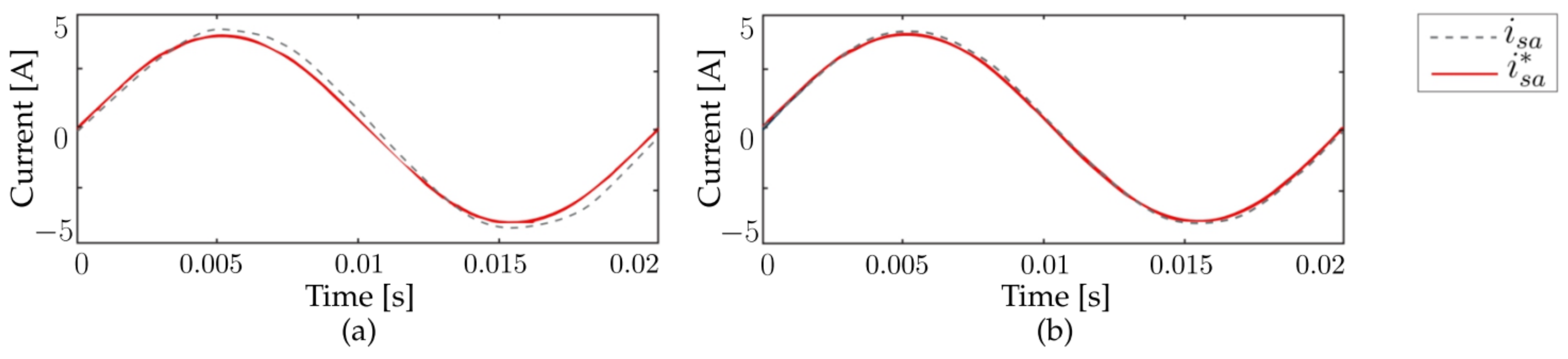
4.1. Steady-State Analysis

The classic SMC and SMC-ERL behaviour is analysed using a reference frequency of $50$ Hz and a reference current amplitude $i_{sa}^{*}=4$ A. In Figure 4, the stator current is denoted $i_{sa}$. In the tests shown in Figure 4, the values $0.4950$ A and $0.3266$ A were computed for the root mean-square error (RMSE) of the classic SMC and SMC-ERL controllers, respectively. It can be observed that the SMC-ERL controller performs better tracking of the current reference compared to the classic SMC. Moreover, it produces less chattering in the stator current. Therefore, it can be observed that the SMC-ERL controller achieves better current tracking than the classic one.

Next, both controllers’ total harmonic distortion (THD) is analysed. For this purpose, $i_{sa}^{*}=3$ A and a frequency of 50 Hz are established. The THD values obtained for the classic SMC and SMC-ERL were 2.52% and 1.28%, respectively.

Considering that the simulation results show that the SMC-ERL controller performs better than the classic SMC, the subsequent tests were conducted using only the proposed SMC-ERL controller.

4.2. SMC-ERL Gain Tuning

For the realisation of these tests, the gains ${\mathcal{K}}_1$, ${\mathcal{K}}_2$ and $\mathrm{\Lambda }$ were varied individually to observe the effect on the stator current tracking for the values chosen in each case. It is possible to notice that the reference tracking was correctly performed in all cases. In Figure 5a,b, it is observed that for small values of the gains $k_{11}=k_{12}$, there is a more considerable difference between the measured value and the stator current reference value that becomes more noticeable as it approaches the peak values. In return, the increase in gain value is accompanied by the rise in chattering. Therefore, a trade-off is established when choosing the value of the gains $k_{11}=k_{12}$. A similar result is obtained by varying the values of the gains $k_{21}=k_{22}$, as can be seen in Figure 5c,d.

The results obtained by varying the value of the gains ${\lambda }_1={\lambda }_2$ are shown in Figure 6. These show that for larger values of the studied gains, the stator current waveform fits better to the reference. However, unlike the gains so far analysed, the magnitude of the chattering is unaffected mainly by increasing the value of ${\lambda }_1={\lambda }_2$.

The statements made from the visual inspection were verified by calculating the RMSE for each test presented. The results shown in

Table 2. RMSE in gain adjustment.

Gain	Values	RMSE (A)
$k_{11}=k_{12}$	1	$0.0553$
	$1.000$	$0.0431$
$k_{21}=k_{22}$	$0.01$	$0.0549$
	100	$0.0311$
${\lambda }_1={\lambda }_2$	100	$0.1378$
	$1.500$	$0.0463$

ratify these statements, since it can be observed that for each case with a higher gain value, the RMSE decreases; therefore, the current tracking method is better.

4.3. Sensitivity Analysis to Parameter Variation

The datasheet provided by the manufacturer of the IM establishes 430 mH as the value of the mutual inductance. This test was carried out to observe the behaviour of the designed SMC-ERL controller in the presence of parametric uncertainties. First, a mutual inductance value lower than the one provided by the manufacturer’s datasheet was chosen, and it was observed that the current tracking persisted. However, at peak values, the stator current briefly exceeded the reference current, adjusting to the same, as shown in Figure 7a. A similar result was obtained by choosing a mutual inductance value higher than that provided by the manufacturer’s datasheet, as seen in Figure 7b. The RMSE values obtained were $0.0629$ and $0.0468$ A for mutual inductances of 230 and 630 mH, respectively. With these tests, it is possible to demonstrate that the designed controller behaves adequately concerning its immunity to the presence of parametric uncertainties.

4.4. Analysis in Response to Frequency Variation of the Reference Current

The stator current tracking test for different frequency values of the reference current can be seen in Figure 8. Different frequency values were chosen to carry out this test. The gain values remained constant in all cases and were determined heuristically.

This test shows that for a given value of the current amplitude, as the current frequency increases, the differences between the measured and reference stator current values at the peaks increase.

These observations were again contrasted with the RMSE, obtaining values of $0.0455$ and $0.0590$ A for frequencies of 50 and 100 Hz, respectively. The RMSE values confirm that the differences between the measured and reference current increase for higher frequencies.

4.5. Analysis of Electrical Frequency Variation

This test was performed to observe the stator current tracking upon an abrupt change in the frequency value (increase or decrease). As shown in Figure 9, the controller momentarily lost the reference tracking with an abrupt change in the frequency value. However, it recovered almost instantaneously. The same test could be repeated after an instant, obtaining the same results. Therefore, it was demonstrated that the designed controller has a fast response to transient changes.

5. Experimental Results

This section presents the results of the experimental validation of the SMC-ERL applied to the current control of a three-phase IM fed by the DMC. For this purpose, an experimental platform whose main components are shown in Figure 10 was used. The DMC was based on SCH2080KE SiC-MOSFETs. The same figure shows the clamp circuit, which provides surge protection for the DMC. The voltage and current sensor boards obtained the magnitudes of the signals and delivered them to the MicroLabBox dSPACE in charge of executing the control algorithms. In turn, the NEXYS 3 field-programmable gate array (FPGA) was used to implement switching algorithms for the SiC-MOSFETs. The signals were transmitted to the bidirectional switches through fibre-optic cables. The IM acts as the load, and the encoder is used to measure the rotational speed of the machine.

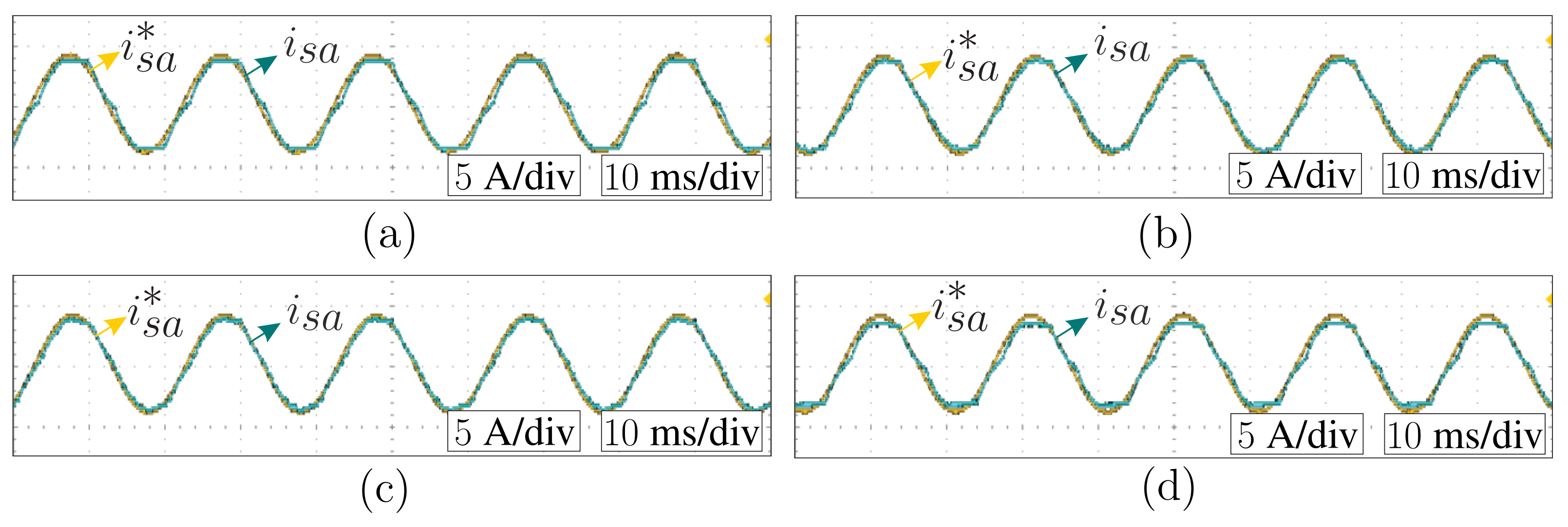
5.1. Steady-State Analysis of SMC-ERL

For the steady-state analysis of the reference stator current tracking $i_{sa}^{*}$, a frequency of 50 Hz and an amplitude of 4 A were used. The gains of both controllers were the same as those used in the simulation environment. In Figure 11 it is possible to observe the behaviour of the designed control algorithms, the classic SMC controller and the SMC-ERL controller, respectively. The experimental results agree with the simulated tests and show that the measured stator current is better matched to the reference value using the SMC-ERL controller. Furthermore, it can be observed that the voltage waveform applied on the load has an approximately sinusoidal shape using the SMC-ERL controller, whereas with the classic SMC controller, the voltage waveform is noisier and less sinusoidal. The same results were seen when calculating the RMSE. The classic SMC gave a value of $0.4950$ A, and the SMC-ERL controller, $0.3266$ A.

5.2. SMC-ERL Gain Adjustments

The experimental validation was carried out identically to the test performed through simulations. For this purpose, the controller gains were adjusted, starting with small values, and one of them was increased, leaving the others constant. The results obtained for the gain adjustment ${\mathcal{K}}_1$ are shown in Figure 12a,b. It is possible to quantify the RMSE values obtained in

Table 3. RMSE in the gain adjustment.

Gain	Value	RMSE (A)
$k_{11}=k_{12}$	1	$0.4699$
	$1.000$	$0.3826$
$k_{21}=k_{22}$	$0.01$	$0.5257$
	100	$0.4663$
${\lambda }_1={\lambda }_2$	100	$0.4467$
	$1.500$	$0.2683$

. Similar results were obtained by varying the values of the gains ${\mathcal{K}}_2$ and $\mathrm{\Lambda }$, as can be seen in Figure 12c,d and Figure 13, respectively.

While it has been shown that the stator current tracking is better at higher gain values, there is a trade-off between gain value and chattering magnitude. In that context, it is not recommended to increase indefinitely any of the gains of the SMC-ERL-based controllers.

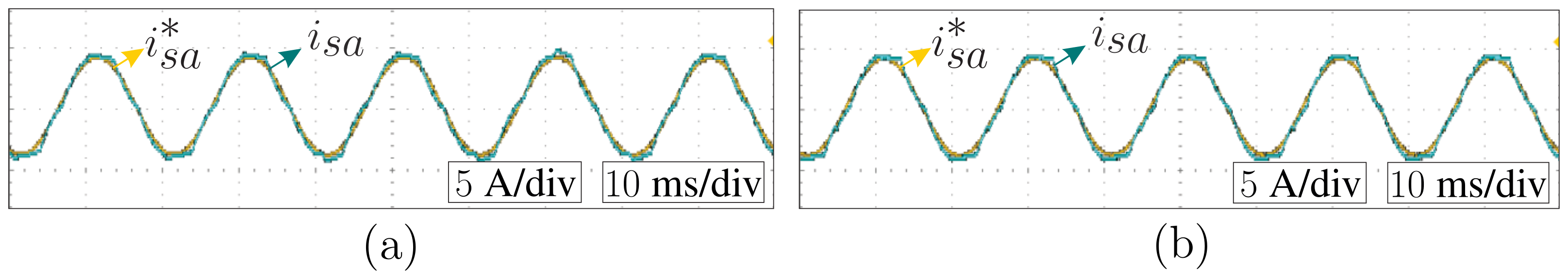
5.3. Sensitivity Analysis to Parameter Variation

The controller’s immunity to parametric uncertainties is a desirable feature of the SMC. Tests were performed by varying the value of the magnetisation inductance to validate this feature, thereby obtaining the results shown in Figure 14. The RMSE values calculated in this case were $0.3454$ and $0.3396$ A for inductances of 230 and 630 mH, respectively. Therefore, even though the value used for the magnetisation inductance parameter was not exact, the reference tracking was established and maintained over time. Note that the variation in $L_m$ implies variation in the whole dynamics, since $f(\mathbf{x},t)$ and g are in terms of this inductance [44]. The simulation and experimental results proved the robustness of the developed SMC-ERL method against parameter variations.

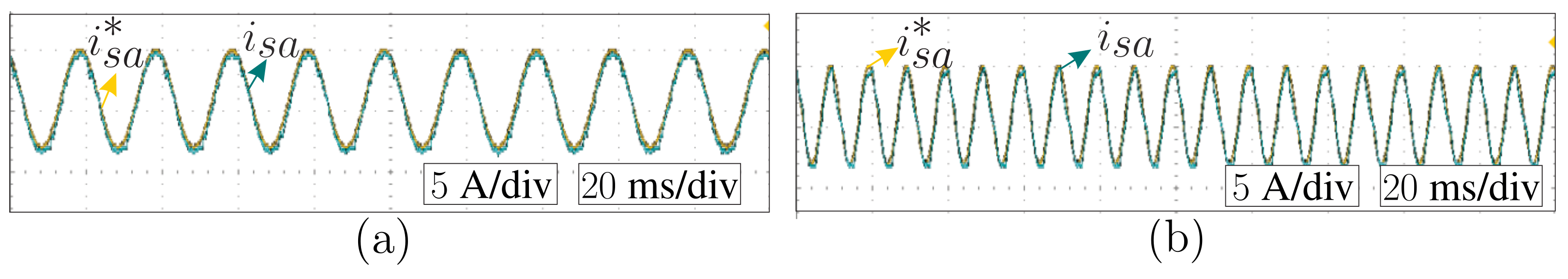
5.4. Analysis against the Variation of Frequency of the Reference Current

Figure 15 shows the analysis of the follow-up of the stator current when varying its frequency from 50 to 100 Hz. The RMSE values obtained were $0.3066$ A and $0.5604$ A for frequencies of 50 and 100 Hz, respectively. Good current tracking was observed in both cases.

5.5. Analysis against Variation in the Electrical Frequency

Abrupt changes in the value of the frequency of the current reference signal were applied to analyse the designed controller’s behaviour under electrical frequency changes, and the controller’s response to these changes was observed. The results are presented in Figure 16. It is possible to observe that when an abrupt change in the frequency of the reference signal occurred (increase or decrease), the measured stator current lost track for a short period of time. However, tracking was again achieved and maintained for the remainder of the test.

The results obtained in the experimental validation present the expected behaviour, since they are similar to those obtained with the simulated tests, even when the quantitative metrics present differences. These differences are entirely attributable to unavoidable measurement errors and inaccuracies in the model of the plant under study. Therefore, the results highlight that the controller’s performance was as expected under the operating circumstances imposed in each case.

6. Conclusions

In this paper, a theoretical study based on computational simulations has been presented, and subsequently, the experimental validation of nonlinear control algorithms based on the sliding mode technique applied to a direct matrix converter with a three-phase IM as a load has been considered. The method uses the exponential reaching law technique to reduce the chattering present in sliding mode-based controllers.

From the results obtained, it can be confirmed that the proposed control strategy is robust to variations in machine parameters and has a fast transient response. In this sense, it is concluded that the control technique presented in this work is attractive as an alternative to the current control techniques usually implemented for three-phase electrical drives powered by matrix converters.

This paper demonstrated that with modifications, the SMC can include more terms to reduce chattering. The comparison between SMC and SMC-ERL gave us the motivation to address an exhaustive comparison of the proposed methods against others, such as FOC, DTC and FCS-MPC, as a near-future research topic. Moreover, this paper opens the door for a niche applications of other nonlinear control techniques, such as higher-order SMC, fuzzy logic and backstepping, in this exciting system.

References

1. Roy, P.; He, J.; Zhao, T.; Singh, Y.V. Recent Advances of Wind-Solar Hybrid Renewable Energy Systems for Power Generation: A Review. IEEE Open J. Ind. Electron. Soc. 2022, 3, 81–104. [Google Scholar] [CrossRef]
2. Islam, M.A.; Singh, J.G.; Jahan, I.; Lipu, M.H.; Jamal, T.; Elavarasan, R.M.; Mihet-Popa, L. Modeling and Performance Evaluation of ANFIS Controller-Based Bidirectional Power Management Scheme in Plug-In Electric Vehicles Integrated With Electric Grid. IEEE Access 2021, 9, 166762–166780. [Google Scholar] [CrossRef]
3. Bento, A.; Paraíso, G.; Costa, P.; Zhang, L.; Geury, T.; Pinto, S.F.; Silva, J.F. On the potential contributions of matrix converters for the future grid operation, sustainable transportation and electrical drives innovation. Appl. Sci. 2021, 11, 4597. [Google Scholar] [CrossRef]
4. Khosravi, M.; Amirbande, M.; Khaburi, D.A.; Rivera, M.; Riveros, J.; Rodriguez, J.; Wheeler, P. Review of model predictive control strategies for matrix converters. IET Power Electron. 2019, 12, 3021–3032. [Google Scholar] [CrossRef]
5. Bogdan, J.D.I.; Wilamowski, M. (Eds.) The Industrial Electronics Handbook; CRC Press: Boca Raton, FL, USA, 2011. [Google Scholar]
6. Rodas, J.; Gregor, R.; Takase, Y.; Gregor, D.; Franco, D. Multi-modular matrix converter topology applied to the six-phase wind energy generator. In Proceedings of the 2015 50th International Universities Power Engineering Conference, Stoke on Trent, UK, 1–4 September 2015; pp. 1–6. [Google Scholar] [CrossRef]
7. Toledo, S.; Gregor, R.; Rivera, M.; Rodas, J.; Gregor, D.; Caballero, D.; Gavilán, F.; Maqueda, E. Multi-modular matrix converter topology applied to distributed generation systems. In Proceedings of the 8th IET International Conference on Power Electronics, Machines and Drives (PEMD 2016), Glasgow, UK, 19–21 April 2016; pp. 1–6. [Google Scholar] [CrossRef]
8. Toledo, S.; Rivera, M.; Gregor, R.; Rodas, J.; Comparatore, L. Predictive current control with reactive power minimization in six-phase wind energy generator using multi-modular direct matrix converter. In Proceedings of the 2016 IEEE ANDESCON, Arequipa, Peru, 19–21 October 2016; pp. 1–4. [Google Scholar] [CrossRef]
9. Gyugyi, L.; Pelly, B.R. Static Power Frequency Changers: Theory, Performance, and Application; Wiley: Hoboken, NJ, USA, 1976. [Google Scholar]
10. Ming, L.; Ding, W.; Gao, Z.; Yin, C.; Chen, M.; Loh, P.C.; Xin, Z. A SiC-Si Hybrid Module for Direct Matrix Converter with Mitigated Current Spikes. IEEE J. Emerg. Sel. Top. Power Electron. 2021, 10, 3805–3817. [Google Scholar] [CrossRef]
11. Toledo, S.; Maqueda, E.; Rivera, M.; Gregor, R.L.; Caballero, D.; Gavilán, F.; Rodas, J. Experimental assessment of IGBT and SiC-MOSFET based technologies for matrix converter using predictive current control. In Proceedings of the 2017 CHILEAN Conference on Electrical, Electronics Engineering, Information and Communication Technologies (CHILECON), Pucon, Chile, 18–20 October 2017; pp. 1–6. [Google Scholar] [CrossRef]
12. Maqueda, E.; Toledo, S.; Gregor, R.; Caballero, D.; Gavilán, F.; Rodas, J.; Rivera, M.; Wheeler, P. An assessment of predictive current control applied to the direct matrix converter based on SiC-MOSFET bidirectional switches. In Proceedings of the 2017 IEEE Southern Power Electronics Conference (SPEC), Puerto Varas, Chile, 4–7 December 2017; pp. 1–6. [Google Scholar] [CrossRef]
13. Taylor, D.G. Nonlinear control of electric machines: An overview. IEEE Control Syst. Mag. 1994, 14, 41–51. [Google Scholar] [CrossRef]
14. Chikondra, B.; Muduli, U.R.; Behera, R.K. Improved DTC technique for THL-NPC VSI fed five-phase induction motor drive based on VVs assessment over a wide speed range. IEEE Trans. Power Electron. 2021, 37, 1972–1981. [Google Scholar] [CrossRef]
15. Desingu, K.; Selvaraj, R.; Kumar, B.A.; Chelliah, T.R. Thermal performance improvement in multi-megawatt power converters serving to asynchronous hydro generators operating around synchronous speed. IEEE Trans. Energy Convers. 2020, 36, 1818–1830. [Google Scholar] [CrossRef]
16. Ni, K.; Hu, Y.; Gan, C. Parameter deviation effect study of the power generation unit on a doubly-fed induction machine-based shipboard propulsion system. CES Trans. Electr. Mach. Syst. 2020, 4, 339–348. [Google Scholar] [CrossRef]
17. Xu, W.; Ali, M.M. One improved sliding mode DTC for linear induction machines based on linear metro. IEEE Trans. Power Electron. 2020, 36, 4560–4571. [Google Scholar] [CrossRef]
18. Taha, W.; Azer, P.; Poorfakhraei, A.; Dhale, S.; Emadi, A. Comprehensive Analysis and Evaluation of DC-Link Voltage and Current Ripples in Symmetric and Asymmetric Two-Level Six-Phase Voltage Source Inverters. IEEE Trans. Power Electron. 2022. [Google Scholar] [CrossRef]
19. Zhang, J.; Li, L.; Dorrell, D.G. Control and applications of direct matrix converters: A review. Chin. J. Electr. Eng. 2018, 4, 18–27. [Google Scholar] [CrossRef]
20. Arnanz, R.; García, F.J.; Miguel, L.J. Métodos de control de motores de inducción: Síntesis de la situación actual. Rev. Iberoam. Autom. Inf. Ind. 2016, 13, 381–392. [Google Scholar] [CrossRef] [Green Version]
21. Alzate, G.A.; Escobar, M.A.; Torres, C.A. Control vectorial de la máquina de inducción. Sci. Tech. 2009, 3. [Google Scholar] [CrossRef]
22. Rodriguez, J.; Cortes, P. Predictive Control of Power Converters and Electrical Drives; John Wiley & Sons, Ltd.: Hoboken, NJ, USA, 2012. [Google Scholar] [CrossRef]
23. Kral, M.; Gono, R. Dynamic model of asynchronous machine. In Proceedings of the 2017 18th International Scientific Conference on Electric Power Engineering (EPE), Kouty nad Desnou, Czech Republic, 17–19 May 2017. [Google Scholar] [CrossRef]
24. Maqueda, E.; Toledo, S.; Caballero, D.; Gavilan, F.; Rodas, J.; Ayala, M.; Delorme, L.; Gregor, R.; Rivera, M. Speed Control of a Six-Phase IM Fed by a Multi-Modular Matrix Converter Using an Inner PTC with Reduced Computational Burden. IEEE Access 2021, 9, 160035–160047. [Google Scholar] [CrossRef]
25. Rodriguez, J.; Garcia, C.; Mora, A.; Flores-Bahamonde, F.; Acuna, P.; Novak, M.; Zhang, Y.; Tarisciotti, L.; Davari, S.A.; Zhang, Z.; et al. Latest Advances of Model Predictive Control in Electrical Drives—Part I: Basic Concepts and Advanced Strategies. IEEE Trans. Power Electron. 2022, 37, 3927–3942. [Google Scholar] [CrossRef]
26. Rodriguez, J.; Garcia, C.; Mora, A.; Davari, S.A.; Rodas, J.; Valencia, D.F.; Elmorshedy, M.; Wang, F.; Zuo, K.; Tarisciotti, L.; et al. Latest Advances of Model Predictive Control in Electrical Drives—Part II: Applications and Benchmarking With Classical Control Methods. IEEE Trans. Power Electron. 2022, 37, 5047–5061. [Google Scholar] [CrossRef]
27. Wang, F.; Mei, X.; Rodriguez, J.; Kennel, R. Model predictive control for electrical drive systems—An overview. CES Trans. Electr. Mach. Syst. 2017, 1, 219–230. [Google Scholar] [CrossRef]
28. Elmorshedy, M.F.; Xu, W.; El-Sousy, F.F.M.; Islam, M.R.; Ahmed, A.A. Recent Achievements in Model Predictive Control Techniques for Industrial Motor: A Comprehensive State-of-the-Art. IEEE Access 2021, 9, 58170–58191. [Google Scholar] [CrossRef]
29. Wei, Y.; Sun, L.; Chen, Z. An Improved Sliding Mode Control Method to Increase the Speed Stability of Permanent Magnet Synchronous Motors. Energies 2022, 15, 6313. [Google Scholar] [CrossRef]
30. Hajihosseini, M.; Lešić, V.; Shaheen, H.I.; Karimaghaee, P. Sliding Mode Controller for Parameter-Variable Load Sharing in Islanded AC Microgrid. Energies 2022, 15, 6029. [Google Scholar] [CrossRef]
31. Luo, B.-Y.; Subroto, R.K.; Wang, C.-Z.; Lian, K.-L. An Improved Sliding Mode Control with Integral Surface for a Modular Multilevel Power Converter. Energies 2022, 15, 1704. [Google Scholar] [CrossRef]
32. Yaramasu, V.; Wu, B. Model Predictive Control of Wind Energy Conversion Systems; John Wiley & Sons: Hoboken, NJ, USA, 2020; ISBN 978-1-118-98858-9. [Google Scholar]
33. Rodas, J.; Martín, C.; Arahal, M.R.; Barrero, F.; Gregor, R. Influence of Covariance-Based ALS Methods in the Performance of Predictive Controllers with Rotor Current Estimation. IEEE Trans. Ind. Electron. 2017, 64, 2602–2607. [Google Scholar] [CrossRef]
34. Rodas, J.; Barrero, F.; Arahal, M.R.; Martín, C.; Gregor, R. Online Estimation of Rotor Variables in Predictive Current Controllers: A Case Study Using Five-Phase Induction Machines. IEEE Trans. Ind. Electron. 2016, 63, 5348–5356. [Google Scholar] [CrossRef]
35. Ayala, M.; Doval-Gandoy, J.; Rodas, J.; González, O.; Gregor, R. Current control designed with model based predictive control for six-phase motor drives. ISA Trans. 2020, 98, 496–504. [Google Scholar] [CrossRef]
36. Liu, J.K.; Wang, X. Advanced Sliding Mode Control for Mechanical Systems; Springer: Berlin/Heidelberg, Germany, 2011. [Google Scholar] [CrossRef]
37. Liu, J.; Gao, Y.; Yin, Y.; Wang, J.; Luo, W.; Sun, G. Sliding Mode Control Methodology in the Applications of Industrial Power Systems; Springer: Berlin/Heidelberg, Germany, 2019. [Google Scholar] [CrossRef]
38. Derbel, N.; Ghommam, J.; Zhu, Q. Applications of Sliding Mode Control; Springer: Berlin/Heidelberg, Germany, 2017. [Google Scholar] [CrossRef]
39. Slotine, J.J.E.; Li, W. Applied Nonlinear Control; Prentice Hall: Upper Saddle River, NJ, USA, 1991. [Google Scholar]
40. Longfei, J.; Yuping, H.; Jigui, Z.; Jing, C.; Yunfei, T.; Pengfei, L. Fuzzy Sliding Mode Control of Permanent Magnet Synchronous Motor Based on the Integral Sliding Mode Surface. In Proceedings of the 2019 22nd International Conference on Electrical Machines and Systems (ICEMS), Harbin, China, 11–14 August 2019; pp. 1–6. [Google Scholar] [CrossRef]
41. Latosiński, P. Sliding mode control based on the reaching law approach—A brief survey. In Proceedings of the 2017 22nd International Conference on Methods and Models in Automation and Robotics (MMAR), Miedzyzdroje, Poland, 28–31 August 2017; pp. 519–524. [Google Scholar] [CrossRef]
42. Fallaha, C.J.; Saad, M.; Kanaan, H.Y.; Al-Haddad, K. Sliding-Mode Robot Control With Exponential Reaching Law. IEEE Trans. Ind. Electron. 2011, 58, 600–610. [Google Scholar] [CrossRef]
43. Casadei, D.; Serra, G.; Tani, A.; Zarri, L. Matrix converter modulation strategies: A new general approach based on space-vector representation of the switch state. IEEE Trans. Ind. Electron. 2002, 49, 370–381. [Google Scholar] [CrossRef]
44. Delorme, L.; Ayala, M.; Rodas, J.; Gregor, R.; Gonzalez, O.; Doval-Gandoy, J. Comparison of the Effects on Stator Currents Between Continuous Model and Discrete Model of the Three-phase Induction Motor in the Presence of Electrical Parameter Variations. In Proceedings of the 2020 IEEE International Conference on Industrial Technology (ICIT), Buenos Aires, Argentina, 26–28 February 2020; pp. 151–156. [Google Scholar] [CrossRef]
Figure 1. Direct matrix converter schematic circuit.
Energies 15 08379 g001
Figure 2. Graphic interpretation of the SMC. (a) State trajectories. (b) Evolution of the state trajectory. (c) Chattering.
Energies 15 08379 g002
Figure 3. Proposed control method based on the SMC.
Energies 15 08379 g003
Figure 4. Simulation of the designed control algorithms. (a) Classic SMC controller. (b) SMC-ERL controller.
Energies 15 08379 g004
Figure 5. Gain adjustment results. (a) K 1 = 1 and (b) K 1 = 1000 . (c) K 2 = 0.01 and (d) K 2 = 100 .
Energies 15 08379 g005
Figure 6. Gain adjustment results. (a) Λ = 0.0001 . (b) Λ = 2000 .
Energies 15 08379 g006
Figure 7. Results obtained from the variation of the parameter L m . (a) L m = 230 mH. (b) L m = 630 mH.
Energies 15 08379 g007
Figure 8. Current tracking results at different frequency values of the reference current. i s a * = 4 A. (a) f = 50 Hz. (b) f = 100 Hz.
Energies 15 08379 g008
Figure 9. Current tracking results visualized as frequency changes. (a) Reference from 20 to 50 Hz and return to 20 Hz. (b) Reference from 20 to 50 and finally 100 Hz.
Energies 15 08379 g009
Figure 10. Experimental test bench.
Energies 15 08379 g010
Figure 11. Experimental results of designed algorithms: (a) Classic SMC. (b) SMC-ERL.
Energies 15 08379 g011
Figure 12. Gain adjustment validation, K 1 and K 2 . (a) K 1 = 1 . (b) K 1 = 1000 (c) K 2 = 0.01 . (d) K 2 = 100 .
Energies 15 08379 g012
Figure 13. Gain adjustment validation, Λ . (a) Λ = 0.0001 . (b) Λ = 2000 .
Energies 15 08379 g013
Figure 14. Results of L m parameter variation. (a) L m = 230 mH. (b) L m = 630 mH.
Energies 15 08379 g014
Figure 15. Current tracking performance. i s a * = 4 A, (a) f = 50 Hz (b) f = 100 Hz.
Energies 15 08379 g015
Figure 16. Current tracking performance compared to reference frequency changes. (a) Reference from 20 to 50 Hz. (b) Reference from 50 to 20 Hz.
Energies 15 08379 g016