Article

On the Kinetic Mechanisms of the Reduction and Oxidation Reactions of Iron Oxide/Iron Pellets for a Hydrogen Storage Process

1
Laboratory of Sorption Processes, Technical University of Applied Sciences, OTH Regensburg, Galgenbergstraße 30, 93053 Regensburg, Germany
2
Regenerative Energy Systems, TUM Campus Straubing for Biotechnology and Sustainability, Technical University of Munich, Schulgasse 16, 94315 Straubing, Germany
*
Author to whom correspondence should be addressed.
Energies 2022, 15(21), 8322; https://doi.org/10.3390/en15218322
Submission received: 3 October 2022 / Revised: 24 October 2022 / Accepted: 2 November 2022 / Published: 7 November 2022
(This article belongs to the Section A5: Hydrogen Energy)

Abstract

:
This work aims at investigating the kinetic mechanisms of the reduction/oxidation (redox) reactions of iron oxide/iron pellets under different operating conditions. The reaction principle is the basis of a thermochemical hydrogen storage system. To simulate the charging phase, a single pellet consisting of iron oxide (90% Fe2O3, 10% stabilising cement) is reduced with different hydrogen (H2) concentrations at temperatures between 600 and 800   ° C . The discharge phase is initiated by the oxidation of the previously reduced pellet by water vapour (H2O) at different concentrations in the same temperature range. In both reactions, nitrogen (N2) is used as a carrier gas. The redox reactions have been experimentally measured in a thermogravimetric analyser (TGA) at a flow rate of 250   m L / m i n . An extensive literature review has been conducted on the existing reactions’ kinetic mechanisms along with their applicability to describe the obtained results. It turned out that the measured kinetic results can be excellently described with the so-called shrinking core model. Using the geometrical contracting sphere reaction mechanism model, the concentration- and temperature-dependent reduction and oxidation rates can be reproduced with a maximum deviation of less than 5%. In contrast to the reduction process, the temperature has a smaller effect on the oxidation reaction kinetics, which is attributed to 71% less activation energy ( E a , Re = 56.9   kJ/mol versus E a , Ox = 16.0   kJ/mol ). The concentration of the reacting gas showed, however, an opposite trend: namely, to have an almost twofold impact on the oxidation reaction rate constant compared to the reduction rate constant.

1. Introduction

The negative effects of climate change are becoming increasingly visible in everyday life [1]. Global energy-related greenhouse and CO2 emissions are the reasons behind this development. Despite periodic flattening, these have increased by an average of 1% per year over the last ten years [2]. To counteract this development, constructive approaches are needed to enable a global transformation of fossil fuel-dominated energy systems into energy- and resource-saving systems. A decentralised “green” energy supply system can be realised by a smart combination of wind, solar and/or bioenergy with efficient energy storage and effective energy recovery solutions. Such a sustainable energy system will enable the transition of various energy sectors such as industrial plants and urban residential areas into green societies [3,4]. The energy carrier hydrogen offers ideal conditions for such a cross-sector “green” energy supply. It can make a substantial contribution to the decarbonisation of stationary energy applications as well as the transport sector [4,5]. Additionally, H2, as a clean energy carrier, has the potential to provide the much-needed flexibility to power systems, acting as a buffer to non-dispatchable renewable energy generation, and therefore, it can play a key role in the seasonal balancing of renewable generation by storing large amounts of it [2].
For the wide application of this potential energy carrier, suitable storage solutions are required. One storage solution is the thermochemical reduction/oxidation of metal oxides ( M n O m )/metals (M) [6,7,8], which can be generally described as follows:
M n O m + m H 2 n M + m H 2 O .
While the reacting solid material does not provide a carrier material for hydrogen, it serves as a kind of catalyst for the oxidation of hydrogen to steam during the charging phase and, later on, for the reduction of steam to hydrogen during the discharging phase. Not only Fe but also other metals, such as Ce, Cu, Mn, Ni, and W, have been tested as reaction masses [9]. Based on a holistic view of the material parameters—availability, costs, reaction kinetics and energy storage density—iron proved to be the most suitable oxide carrier material [6,9,10,11].
At the beginning of the 20th century, the fundamentals of the iron redox process were used for the production of hydrogen, whereby the process was also given the name “steam–iron process” [12,13]. Nowadays, the reduction of iron oxide is mainly used in iron production [14,15]. Within the so-called direct reduction process, iron ore is reduced to metallic iron by means of a H2/CO gas mixture. In view of the high economic importance of iron, the reduction behavior of iron oxides is a frequently studied topic in ferrous metallurgy [14,15,16].
In general, the steam iron process can be considered as a heterogeneous non-catalytic gas-solid reaction [17], in which the charging and discharging phases must be considered separately. The endothermic charging phase, in which the reduction of magnetite (Fe3O4) to Fe takes place, can be described as follows:
F e 3 O 4 + 4 H 2 3 F e + 4 H 2 O .
Hydrogen reduces Fe3O4 first to wustite, simplified as FeO, and then to Fe. Hereby, H2 is oxidised to steam. The corresponding oxidation reaction, which follows also the two-stage reaction principle, is given by:
3 F e + 4 H 2 O F e 3 O 4 + 4 H 2 .
If the mass ratio of H2 to Fe in Equations (2) and (3) is considered, a theoretical maximum storage of H2 in Fe of 4.8   w t % can be estimated, which corresponds to a gravimetric energy storage density (ESD) of 1.6   kwh / ( kg Fe ) . Considering a tubular reactor being filled with spherical storage pellets each having a diameter of d = 12   mm , and made of a mixture of 90   w t % hematit and 10   w t % stabilisation material, the fixed-bed porosity can be estimated to 36%. The resulting volumetric ESD is then estimated to be 2.8   kwh / ( L b u l k ) [18].
This exceptionally high ESD, together with the cost advantage of the storage material, offers an excellent basis for the development of an efficient hydrogen storage unit. Accordingly, several research groups have been conducting research and development tasks on this specific field. A major focus of previous research is the intermediate storage of hydrogen in a rechargeable oxide battery (ROB) with an operating temperature of 800   ° C  [19,20]. By applying 30% of 8 YSZ to the iron oxide form, the highest number of 200 stable cycles, each 70   min long, was obtained. However, these promising results have been realised at the cost of a remarkable reduction in the ESD from 1340 to 900   Wh/kg due to the excessive amount of additives required [21].
Furthermore, a reformer steam iron cycle, developed by an Austrian research group, enables the production and storage of hydrogen out of bio-resources such as biogas or gasified biomass at an operating temperature of 800   ° C [9]. A 10   k W th laboratory prototype, which is filled in with 18   kg of an oxygen carrier material, was presented [22]. The oxygen carrier material was applied in powder form and consists of 80% Fe2O3 and 20% Al2O3. More than 20 redox cycles could be performed in this prototype. With closing the system during the oxidation phase, the researcher showed with another test rig the possibility of producing a pressurised hydrogen up to 95 bar [23]. A further research group from the Tokyo Institute of Technology has also studied the effect of applying different additives such as Al, Cr, Cu, Ni, Rh and Zr on the storage medium in a temperature range between 300 and 380   ° C [24,25]. Iron oxide samples with a mass of 0.2   g (each comprising 5   mol% of one additive) were processed in a quartz tube reactor (length = 60   cm , i.d. = 200   mm ) with reduction mixtures of CO and H2 as well as methane. Steam with argon as a carrier gas was used as an oxidation gas. A total of 13 cycles were studied, in which Cr cations have demonstrated a prevention of the sintering of iron species during the redox reactions. In addition, Cu and Ni species as well as Rh were proven to be effective additives for hydrogen formation by the oxidation of iron with steam.
It can be concluded that in sum, the redox storage of H2 is a promising concept due to the strong bonding of hydrogen and the high ESD [26,27]. In addition, the hydrogen is not directly stored, which is a substantial safety advantage if compared with compressed or liquified hydrogen. Furthermore, the redox storage principle offers promising integration opportunities with industrial processes operating at elevated temperatures, such as hydrogen pyrolysis [28] or the generation/combustion of H2 using solid oxide fuel cells [29].
The overarching focus of our research group is to develop a redox storage technology based on stable iron oxide pellets [30] as a stand-alone renewable energy storage and supply system for urban quarters and industrial facilities. More about the storage process can be read elsewhere [18].
In this work, the kinetics of both reduction and oxidation (redox) reactions on an iron oxide/iron pellet have been experimentally investigated under different isothermal conditions and different concentrations of the respective reacting gas. In addition, a thorough literature review has been carried out on the existing reactions’ kinetic models and their applicability to describe the obtained experimental results. The work is devoted to gain a more systematic understanding of the kinetics of the steam-iron reactions according to (Equations (2) and (3)). To this aim, the existing kinetic models for both reduction and oxidation phases are presented and examined against our own experimental data. Both temperature and concentration dependencies of the velocity rate constants have been estimated and two conversion rate correlations for subsequent modelling activities have been suggested for both reduction and oxidation reactions on the investigated iron oxide pellets.

2. Kinetic Models

Kinetic models of chemical reactions are fundamental for the design, scale-up, optimisation, and industrial application of the reactor process. They depend on the reaction conditions such as temperature, material, particle size, flow rate, concentration, etc. For the formulation of a useful model, the prevailing chemical reaction must be correctly determined. There are many ways of classifying chemical reactions. Probably the most widely used scheme is the subdivision according to the number and type of phases involved. Generally, a differentiation is made between homogeneous and heterogeneous systems. If the reaction takes place in only one phase, it is called homogeneous. In case there are at least two phases, the reaction is termed as heterogeneous.
Additionally, the reaction can be specified according to the phase of the reactants, for example fluid–fluid or solid–fluid. On top of these classifications, the reactions can be of catalytic or non-catalytic type. Catalysts, as foreign agents that are neither reactants nor products, have a significant influence on the reaction rate. They act as intermediaries either to accelerate or to hinder the reaction. Non-catalytic reactions take place without additional substances [17,31].
In general, solid–fluid, especially solid–gas reactions are very important in many chemical and metallurgical processes, such as the reduction of oxide ores, coal gasification, roasting of sulphides and the like [14,32,33]. To study their kinetics, it is essential to define a corresponding mathematical model based on physical and chemical principles. To describe these models, a quasi-steady state is assumed, which means that the reaction is assumed to consume all the gaseous reactant supplied to the solid surface. Generally this is described with the equation:
aA ( g ) + bB ( s ) cC ( s ) + dD ( g )
Here, A(g) is the reactive gas, B(s) is the active chemical solid component, C(s) is the solid product and D(g) is the gaseous product. The stoichiometric coefficients for reactants and products are given with a, b, c and d.
In order to describe the basics for the kinetic mechanisms discussed later, only the reduction of iron oxide from the reversible redox process is described in more detail below. A schematic representation of the sequential steps taking place during the reduction of a porous iron oxide particle can be seen in Figure 1. Here, the reducing gas flows through the cracks or open pores in the pellet and forms individual iron oxide regions, thus creating a flowing boundary layer. Mass transfer between the moving gas phase and the oxide surface takes place by transporting the reacting gases through this boundary layer, the so-called film layer. With the progress of the reduction phase, the reducing gas diffuses through the already reacted zone, also known as macro (1) and micro (2) pores. At the solid/gas interface, the iron oxide reduction reaction (3) described by Equation (2) takes place. This includes the adsorption of the reducing gas, the removal of oxygen from the crystal lattice (4), the formation and growth of nuclei of the reaction products wuestite or iron and finally the desorption of the oxidised gas molecules (H2O) from the surface of the solid. The oxidised gas exits the pellet in the same way (5,6). If the kinetic rate-determining reaction is in the scenarios (1,2,5,6), it is a diffusion-limited reaction, making the overall reaction diffusion- or transport-controlled. However, if it is in the scenarios (3,4), the process becomes reaction-controlled [17,32]. A more detailed description of the physical and chemical steps taking place during such a reaction can be read in [32,34,35].
In the following subsections, the structural–physical principles utilised for the detailed description of the dynamic behavior of the reacting pellet are first derived, which is followed by the methodology of calculating the temperature- and concentration-dependent kinetic parameters.

2.1. Geometry Model

For the solid–gas system, the general molar balance equation for the reactants j = A, B (see Equation (4)) can be formulated as follows [34,36]:
n j t = u c j + D c j ± R j · d V p
The diffusive mass transport of the reactants can be expressed by the vector of the diffusive mass flow density, which is mathematically and physically defined as the product of the molecular diffusion coefficient and the vector of the concentration gradients of the species j D c j , which is also called the 1st Fick’s law of diffusion [37]. Moreover, since the inflowing and outflowing mole streams are the same (4 moles of H2 against 4 moles of H2O as described by Equation (2)), the convection term u c j can be neglected. The mass of species j formed by the chemical reaction in the balance volume is described by the rate of change of the mass R j .
Assuming a constant radius for the spherical pellet during the reaction d r p d t = 0 , the differential of a porous spherical shell volume can be described as d V p = ε p 4 π r p 2 d r p . Here, ε p specifies the volume fraction that the respective reactant j occupies on average inside the reaction volume. It is then possible to divide Equation (5) by d V p and add the concentration c j = n j V p to the accumulation term:
c j t = D c j + R j
With the assumption of a constant effective diffusion coefficient D e of the gas A through the product layer B, the equation can be reduced to:
c A t = D e Δ c A + R A
The variation of mass in the gas phase according to
H 2 + O 2 H 2 O + 2 e
is due to the mass change of the solid phase according to
Fe 3 O 4 + Fe 2 + + 2 e 4 FeO
FeO Fe + O .
Including the stochiometric coefficients according to Equation (4), the mass change of the solid B can thus be described, assuming irreversibility and first-order rate in the concentration of the gas reactant, as follows [38,39]:
d c B d t = b R B
with
R B = f ( α ) · c A ,
where c A is the reaction gas concentration and f ( α ) describes the amount of solid B per unit volume of the solid. This function can be expressed after meeting some assumptions concerning the behavior of solid matrix during the conducted reaction. In the literature [40,41,42,43], the following four different functional expressions are present:
  • In Reaction order models, the reaction rate is proportional to the concentration, where the remaining amount or fraction of the reactant is raised to a particular power (integral or fractional), which represents the reaction order n RB . The general formulation for a reaction-based model is:
    f ( α ) = ( 1 α ) n RB
  • Geometric contraction models assume that the adsorption and desorption of the reaction gas occurs uniformly on the surface of the particle. The reaction rate is controlled by the resulting expansion of the contact area towards the centre of the reactant. Assuming that all particles have the same shape and size, this model is easy to parameterise and shows good agreement for metal oxide/metal redox systems. The two relevant kinetic parameters, the generalised rate constant and the morphology n GC (cubic, cylindrical, spherical), can be determined by fitting a single isothermal curve. In general, this can be described with the following algebraic equation:
    f ( α ) = ( n GC + 1 ) ( 1 α ) n GC / ( n GC + 1 )
  • Diffusion models describe complex concentration equilibrium processes through porous solid matrices or simply pore diffusion, which can play an important role in gas–solid reactions. If the reacting solid B has a porosity ( 1 ε ), the description of diffusion through the micro- and macro-pore volume is necessary for the reacting gas A to access the surface of the solid B; the removal of the gaseous product D also occurs in the same way. However, pore diffusion can also be an important component in the reaction of non-porous solids. If the solid product layer C formed is itself porous, the supply of the gaseous reactant A and the removal of the gaseous product D can take place by diffusion through the porous product layer. Depending on the model used, e.g., Gingstling–Brounshtein, Jander or Chou, the mathematical description differs and will be considered in more detail later.
  • Nucleation and nuclei growth models describe the formation and growth of nuclei, which are finite quantities of the product inside the reactant lattice. This includes crystallisation, crystallographic transition, decomposition, adsorption, hydration and desolvation. In general, the rate-controlling step can be the solid diffusion or movement of the interface.
For modelling the structural change of the reaction mass inside the pellet depending on the reaction progress of the heterogeneous, non-catalytic redox reaction, various models can be found in the literature [17,37,44]. Among these models, it can be distinguished between porous and non-porous reaction solid models. Depending on the structural model used, some of these functional mechanisms are applied or even combined, which implies the selection of the appropriate initial and boundary conditions for Equation (7). To formulate an adequate model for describing the complex structure and, consequently, the behavior of the iron oxide pellet during the reaction, the following assumptions deem necessary:
  • Isothermal condition dominates d T / d t = 0 ;
  • Based on Equations (2) and (3), equimolar counterdiffusion is valid n A = n D ;
  • Reactions proceed independently and without interaction between the gaseous species;
  • No crack formation occurs during the reaction;
  • Pressure is uniform inside and around the pellets;
  • Pellet has a uniform and constant porosity d ε / d t = 0 ;
  • Chemical reaction-controlled process inside each grain is reversible and proceeds topochemically.
The simplest structural model, described in this work, is the progressive-conversion model (PCM). PCM assumes that, according to Equation (4), the reaction gas (A) enters the solid (B) at any time and reacts there. If the diffusion rate through the pores of the particle is much higher than the reaction rate D e > > R A , the concentration profile of the reaction gas in Equation (7) will be uniformly distributed over the particle 2 c A x i 2 = 0 .
Consequently, the chemical reaction R A is the only step in the PCM that controls the molar mass change, as illustrated in Figure 2a. Assuming that the concentration of the reaction gas is so high that it remains unchanged during the process d c A d t = 0 , and assuming a first-order reaction takes place inside the solid B, the molar mass consumption of component B can be described (see Equation (11)) as [17]:
d n B d t = b d V p k c A = ε 4 π r p 2 b k c A d r p
The analytical solution for the consumption of component B ( α B , PCM ( t ) ) of this equation is:
α B , PCM = t τ PCM τ PCM = ρ B b a V k PCM c A .
where ρ B is the molar density of the reactive component in the solid B, k PCM is the reaction rate constant, c A is the molar concentration of the reaction gas, a V is the specific surface of the particle (area per unit volume) which remains constant during the proces and τ PCM is the time needed for completing the reaction. Assuming a constant reaction gas concentration inside the entire particle (equal to that in the bulk) and a first-order reaction at the surface of the reaction material, the PCM is the choice to describe leaching processes [44].
In order, however, to model the kinetics of the redox reactions, most of the literature reported that a concentration change over the pellet radius must be assumed d c A ( t ) d r 0 [17,33,34]. Having a metal oxide reacting with a reactant gas, the reaction zone changes or moves from the outer shell of the solid material towards its interior sections during the reaction and, consequently, the gas concentration does change as it continues to react with the shrinking product layer. Such a behavior can be described with the so-called shrinking-core model (SCM). SCM describes an active pellet with a changing reaction zone A c = 4 π r c ( t ) 2 . The reaction takes place, first, on the outer skin A p = 4 π r p 2 of the particle and then moves into the solid. This leaves behind a completely transformed material as well as the inert solid material. This is usually referred to as “ash”. At any time, there is an unreacted core of material that shrinks during the reaction, as illustrated in Figure 2b [17].
The authors of [16,17], have sliced and examined the cross-section of partly reacted solid particles and reported that the unreacted solid material inside the grains are surrounded by a layer of ash. The unreacted core may not always be as sharply defined as the model assumes it; nevertheless, the literature do recommend the SCM for describing the redox behavior of metal oxides [17,33,45,46,47]. The main advantages of the SCM are the simple parameterisation and the existence of an analytical solution for the particle conversion, provided that the gas concentration surrounding the particle (inside the edges or the bulk phase) is constant, i.e., for r > r p d c A d t = c A , Bulk = c A . It also provides an analytical function for the global reaction rate of the entire pellet as a function of the reaction gas concentration as well as the reaction temperature. This is quite useful, especially when the particle model needs to be coupled with a reactor model that is more complex than a simple plug flow [39].
To describe the particle model, the different kinetic mechanisms must be considered. SCM consists of three kinetic control mechanisms, which results from Equation (7) [36] and are described briefly in the following paragraphs:
(1) Diffusion of the reacting gas through the gas film layer (boundary condition) at the corresponding mass transfer coefficient β m s , also termed as the film theory,
D e d c A ( t ) d r | r = r p = β c A c A ( t ) | r = r p t > 0
d n A d t = 4 π r c ( t ) 2 β c A c A | r = r p
(2) Diffusion through the porous product layer (ash layer) with the effective diffusion coefficient D e m 2 s
d n A d t = 4 π r c ( t ) 2 D e d c A d r | r = r c ( t )
(3) Chemical reaction for an irreversible first-order reaction with the kinetic rate constant k m s
d n A d t = 4 π r c ( t ) 2 k c A | r = r c ( t ) .
The concentration gradient d c A d r in the formed product layer can be derived from the molar balance in spherical coordinates by neglecting the convection and reaction terms and assuming pseudo-stationary conditions, as follows:
0 = c A = d 2 c A d r 2 + 2 r d c A d r
Equation (21) is also known as Fick’s second law of diffusion. Applying the boundary conditions for r = r p c A = c A | r = r p and for r = r c ( t ) c A = c A | r = r c ( t ) and carrying out a twofold integration of Equation (21) results in the following expression for the radius dependency of the gas concentration:
c A ( r ) = c A | r = r c ( t ) + c A | r = r p c A | r = r c ( t ) 1 r c ( t ) r 1 r c ( t ) r p
The concentration gradient at the point r = r c ( t ) can be expressed as follows:
d c A d r | r = r c ( t ) = c A | r = r p c A | r = r c r c ( t ) 1 r c ( t ) r p
By substituting Equations (18)–(20) and reformulating it, the surface concentration c A | r = r c ( t ) as a function of r c ( t ) is obtained as follows
c A | r = r c ( t ) = c A 1 + k β r c ( t ) r p 2 + k r c ( t ) D e 1 r c ( t ) r p
Together with Equation (20), the time rate of the converted molar mass of A for a spherical pellet with film and ash diffusion as well as chemical reaction is obtained:
d n A d t = 4 π r c ( t ) 2 k c A 1 + k β r c ( t ) r p 2 + k r c ( t ) D e 1 r c ( t ) r p
A structural study of the pellet requires an expression for r c ( t ) as a function of time. The following correlation exists between the time derivative of the converted solid B and r c ( t ) :
d n B d t = 4 π r c ( t ) 2 ρ B M B d r c ( t ) d t = b d n A d t
Finally, the shrinking unreacted core can be described by applying the stoichiometric coefficients from Equation (4) as follows:
d r c ( t ) d t = c A c B , 0 b k 1 + k β r c ( t ) r p 2 + k r c D e 1 r c ( t ) r p
M B k g mol stays for the molar mass of solid B, b ( ) for its stoichiometric coefficient and ρ B k g m 3 for its density. If the gas inflows continuously, c A can be assumed to be constant in time and position. With the relationship between the degree of conversion of the solid α B and r c
α B ( t ) = 1 c B ( t ) c B , 0 = 1 r c ( t ) r p 3
d α B d t = 3 r p r c ( t ) r p 2 d r c ( t ) d t = 3 r p 1 1 β + 1 k 1 α B 2 / 3 + r p D e 1 α B 1 / 3 1 b c A c B , 0
the function f ( α B ) for the SCM is defined as follows [34,36]:
f ( α B ) = 1 b c B , 0 c A d α B d t
As long as an adequate flow around the pellet is provided, the mass transfer β > > k . Applying this condition in Equation (31) results in:
f ( α B ) = 3 r p k 1 α B 2 / 3 + r p 2 D e 1 α B 1 / 3 1
The overall process rate is determined by the slowest of the two sequential mechanisms, which take place one after the other during the reaction. In other words, if the diffusion through the porous solid layer is the rate-controlling mechanism, the following applies:
1 k 0 f ( α B ) = D e r p 2 3 1 α B 1 / 3 1
In case the chemical reaction is considered to be the rate-controlling mechanism
1 D e 0 f ( α B ) = k r p 3 1 α B 2 / 3
With the effective diffusion coefficient D e , it is possible to describe the resistance of the ash macro pores to the fluid flow in a simplified way. In general, two types of the pores must be considered: pores that are formed during the reaction and those that are available in the raw material.
Different sizes and shapes of these pores lead to different diffusion mechanisms for the reaction gas flow [48]. If the mass transport in the marco pores is the rate-limiting step, it is possible to describe the reaction process using the SCM. In case of high porous masses, which consists of small particles, the effect of gas diffusion as well as the structural properties, such as diameter, porosity and tortuosity, becomes more important. The sharp boundary between the reacted and the unreacted zone can no longer be confirmed for such reaction masses [49,50]. In order to integrate additional reaction zones of particles in the porous mass, the well-known grain model (GM) is applied.
With the GM, not only the diffusion through the formed product layer is taken into account but also the structure of the unreacted solid particles. The gas penetrates through the pores and reacts on the grains’ surface, as shown in Figure 1 and Figure 2c. According to Szekely [51], the solid reactant comprises micro spherical grains, with a reacting core that shrinks as long as the reaction continues. These grains are assumed to be dense and fine with a constant radius r g . Structures of this type can be observed in many porous materials [35,52]. Complementary to the derivation of the SCM in Equation (31), which describes the reaction behavior of one grain, a finite number of micro grains is integrated into the equations to describe the GM, which increases, however, the numerical effort. The reader is referred to [34,39,49,53] for a detailed derivation of the GM.
So far, a general description of the reaction behavior on one pellet was derived, on which basis the prevailing dominant mechanism can be determined, i.e., whether the process is diffusion or chemical reaction dominated. In each case, the relevant kinetic parameters can be estimated.

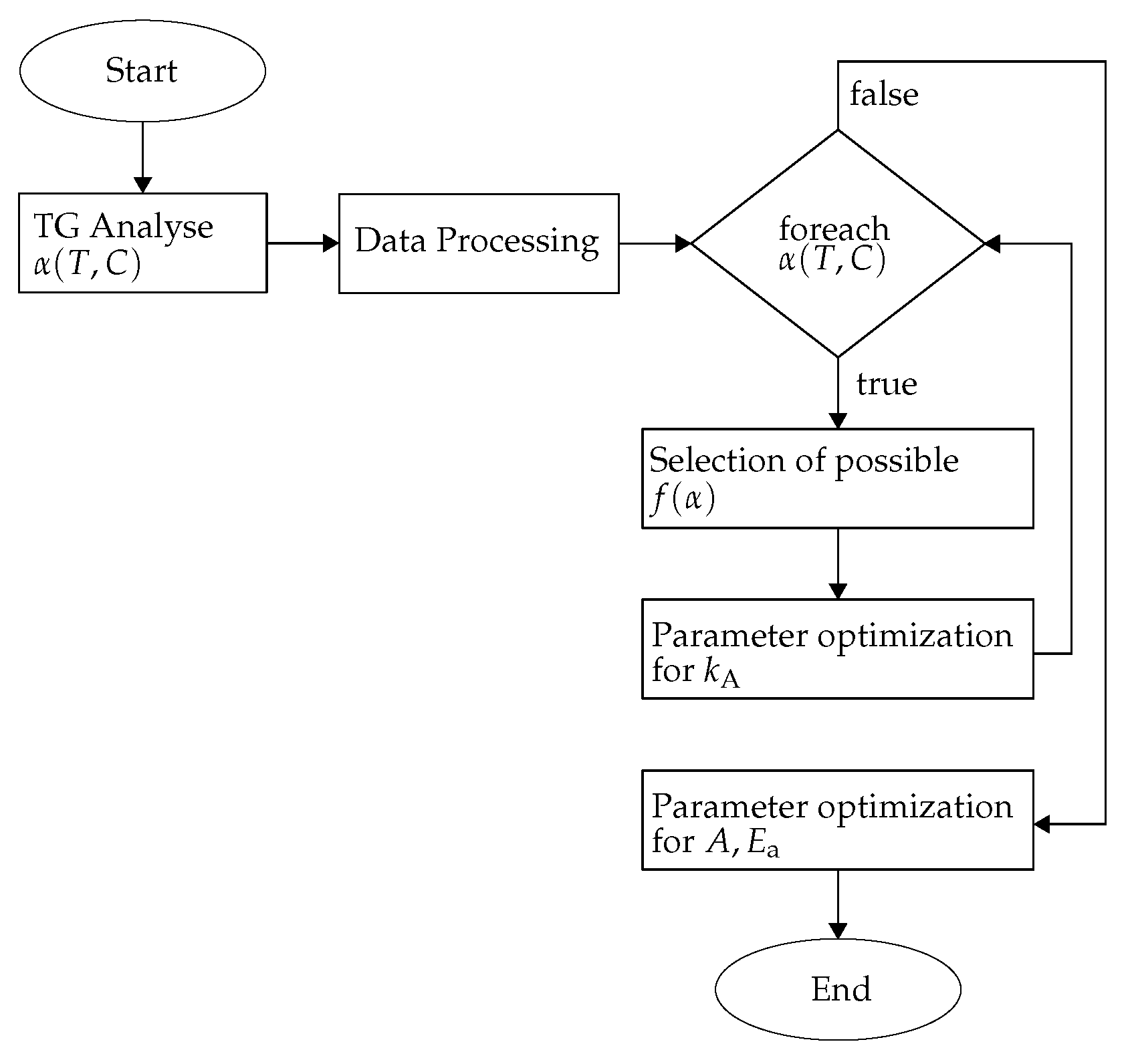
2.2. Estimation of the Kinetic Parameters

In order to investigate the influences of the different reaction conditions, a number of independent algebraic equations have been presented in the literature, which are useful for describing the process within a certain range of reaction conditions [40,54,55,56,57]. The basis for this is the general description of the solid-state reaction rate:
d α d t = k A · f ( α ) ,
where the concentration and temperature dependence is described by the modified Arrhenius rate constant k A 1 s , and the degree of conversion is defined f ( α ) ( ) by an algebraic equation, which represents a physical approximation of the kinetic model and is already discussed in Section 2.1. Exchanging k A by the modified Arrhenius equation results in:
d α d t = A e E a R T C n k A · f ( α )
with α as the reacted fraction at time t, E a as the activation energy, A as a pre-exponential factor of the Arrhenius relationship, and T as the absolute temperature. In addition, the reaction gas concentration C appears, which is raised to an empirical exponent n [58,59,60], which has to be determined by fitting the experimental data to Equation (35).
The algebraic equation f ( α ) is generally classified based on the graphical shape of their isothermal curves or on their mechanistic assumptions. Based on the shape of the isothermal curves of ( d α / d t vs. α ), the kinetic models can be grouped into acceleratory, deceleratory, constant/linear, or sigmoidal models (see Figure 3). Acceleratory models are those in which the reaction rate ( d α / d t ) is increasing as the reaction proceeds (nucleation models). Similarly, deceleratory reaction rates decrease with the reaction progress (phase boundary controlled reaction models or diffusion models). The reaction rate remains constant for linear models (reaction order-based models), while sigmoidal models show a bell-shaped relationship (nuclei growth models).
The mechanistic assumptions f ( α ) evaluated from the plot α vs. t are divided into the already discussed physical processes: Nucleation and nuclei growth (mainly represented by the Avrami–Erofeev equation), progressive conversion (reaction order-based models) as well as diffusion and geometrical contraction [40,61]. The methods for graphical presentation are easy means of visually determining the most appropriate model for a particular dataset. An extraction of the most commonly used kinetic models is presented in Table 1. A more detailed description can be read in [40].
For the parametrisation of the mechanistic models, it is common to use the “model-fitting” method [62,63]. Based on the fitting method, f ( α ) as well as k A can be determined by fitting the integral form of Equation (34), which is described by
0 α d α f ( α ) = k A 0 t d t
g ( α ) = k A t
against the experimental data, which represents the mass change of the sample. The integral form g ( α ) can be determined by integrating the kinetic models of f ( α ) listed in Table 1. By means of a mathematical optimisation method, the activation energy E a can, subsequently, be determined by using the calculated rate constant k from the isothermal experimental data [57].
For the purpose of completeness, the model of Sestak and Berggren [64] should be mentioned here, which showed that it is possible to express the integral form of g ( α ) in a general analytic form that represents all models in a single general expression:
g ( α ) = α m ( 1 α ) o [ l n ( 1 α ) ] p
where m, p and o are constants with the listed possible combinations in Table 2 along with the most suitable application fields of each mechanistic model.
By assigning empirical values for these three variables, the listed physical models in Table 1 can be obtained [64]. An overview of more parameter values and their combinations for more models can be read elsewhere [65].
In order to evaluate the reaction models based on the measured isothermal gravimetric kinetic data, the instantaneous reduction/oxidation fraction α E ( t ) is defined by Equation (39) as the instantaneous mass change of the sample m ( t ) relative to its initial mass m 0 divided by the final mass change m reached after a given maximum reaction time.
α E ( t ) = m 0 m ( t ) m 0 m
The smallest representative investigation unit of a gas–solid reaction system is the interaction of a single particle with a moving gas stream. Since the investigation of single-particle systems is more transparent and the results can be generalised, at least in principle [34], to more complex multi-particle arrangements, a single-pellet measuring device will be described in the following section.

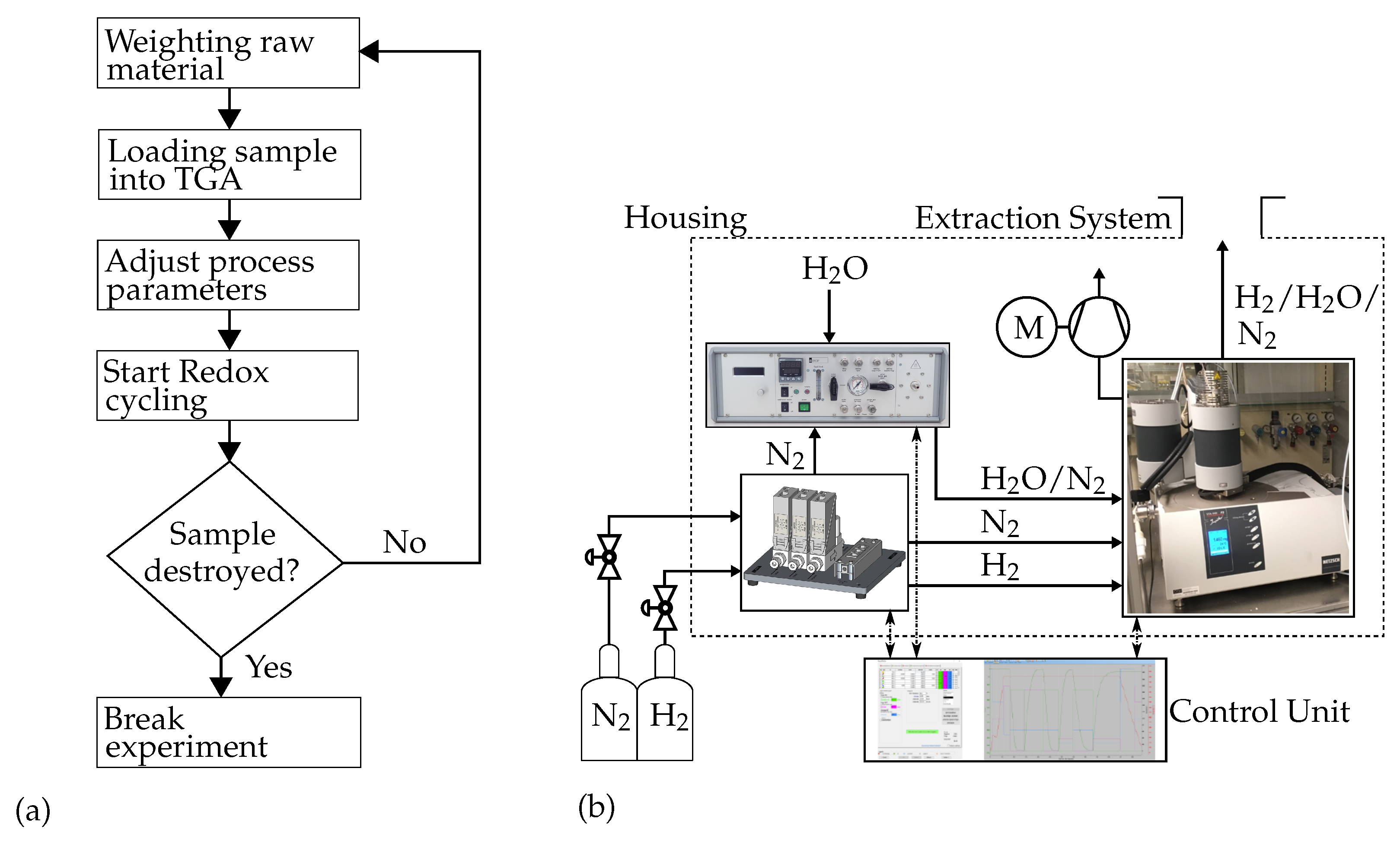
3. Materials and Methods

For investigating the solid–gas redox reaction kinetics in this work, the so-called “engineering approach” is followed, in which a relatively big sample mass is investigated under well-defined external boundary conditions; namely, temperature and gas concentration, in order to obtain the necessary information for the later practical application of the process [50]. A commonly used methodology for such an engineering approach is the determination of the reaction kinetics by means of a thermogravimetric analyser. The set-up used to investigate the iron oxide samples is illustrated schematically in Figure 4, where a hydrogen-compliant thermogravimetric analyser (STA 449-F3, NETZSCH Gerätebau GmbH, Selb, Germany) forms the core component.
The reduction of the iron oxide pellet is triggered by flowing a mixture of nitrogen and hydrogen into the TGA device, where the sample is placed. Different gas mixtures are adjusted by means of a mass flow controller for each gas (EL-FLOW, Bronkhorst, Kamen, Germany) and fed into the TGA device. The oxidation of the previously reduced samples takes place in an H 2 O-H 2 gas mixture atmosphere. The required steam is produced in a steam generator (DV2MK, aDROP Feuchtemeßtechnik GmbH, Fürth, Germany) and transferred to the TGA by means of a heated metallic hose to avoid condensation. Furthermore, a vacuum pump is used to evacuate the experimental setup after each experiment for safety reasons. The measured values of the experimental setup are stored locally on the measurement computer with a sampling rate of 200 points /   min . The accuracies of the applied devices are listed in Table 3.
The investigated sample, based on the recipe of [30], was acquired from the company, Nacompex GmbH, Bad Saarow, Germany. The almost spherical sample consists of a mixture of 90% hematite (Fe2O3) and 10% support material of high-alumina cement [66]. The main function of the support material is to ensure a high dispersion and a high mechanical strength of the pellet. After mixing and shaping processes, the pellets were dried for 28 days under ambient conditions before they were sintered at 950   ° C for 3   h . The investigated sample has a diameter of d s 12.7   mm with a total mass of m s = 3658.5   mg .
Before the very first reduction reaction, the raw sample consists of 90% Fe2O3, which is reduced to Fe using H2. In the subsequent reactions, and because of the adjusted operating conditions (Table 4), Fe can only oxidise to Fe3O4 as can be observed in Section 4.1. From there on, Fe3O4 is converted into Fe and vice versa. More details on this conversion can be read in [67].
As described before, during the experimental campaign for the determination of the reaction kinetics (see Figure 4), the molar concentrations for reduction and oxidation were changed according to Table 4 for the different redox runs (ro 1 –ro 3 ).
The oxidation atmosphere of ro 3 results from the maximum allowed steam concentration for the safe and accurate operation the STA device. At higher concentrations, undesired condensation may take place inside the weighing section of the STA.
Previous studies have reported that the iron composite material can sinter if repeated reactions are performed above an oxidation temperature of 800   ° C  [18,67]. For this reason, the reduction/oxidation investigations have been carried out under the isothermal conditions of 600   ° C , 700   ° C , and 800   ° C .

4. Results and Discussion

This section is divided into two main subsections: namely, Reduction and Oxidation. At the beginning of each subsection, an algebraic equation from Table 1 is fitted to the experimental values using the model-fitting method for isothermal experiments [41]. As previously explained, the kinetic parameters, activation energy E a and Arrhenius’ pre-exponential factor A, are determined for the respective redox reaction by means of a mathematical optimisation fitting to the algebraic equations. To solve these non-linear curve-fitting problems (data fitting), the least squares method is applied in MATLAB R2019b [68]. Generally formulated, the optimisation problem for the velocity rate constant is
min k A F exp d α ( k A ) d t 2 2 = min k A i F exp , i d α i ( k A ) d t 2
and for the activation energy is
min A , E a F k A , exp f ( A , E a ) 2 2 = min A , E a i F k A , exp , i f i ( A , E a ) 2
with F exp representing the experimental data, d α d t as well as the searched coefficient k A from Equation (34). F k A , exp is a function of the determined velocity rates from the experimental data and f ( A , E a ) with the searched parameters A , E a for the Arrhenius formalism of Equation (35). A flowchart describing the estimation methodology for the kinetic parameters is depicted in Figure 5.
The absolute deviation (AD) between the experimentally measured reduction or oxidation fraction α Exp and the mathematically fitted values α Fit is defined by Equation (42). For better reading and interpreting the diagrams, AD is expressed in (%) rather than in a dimensionless fraction.
AD = α Exp α Fit · 100 %

4.1. Reduction

As described previously, the reduction behavior of a metal oxide is a complex thermochemical gas–solid process, which has been in depth investigated with the main target to improve the theoretical models and the applied algebraic rate equations [32,34,40,69]. In this subsection, the focus is specifically on the reduction of iron oxide using hydrogen, for which a summary of the relevant literature can be found in Table 5. In the following, the individual results of the literature review are discussed, using the symbols from Table 1.
The literature review reveals that although some researchers have chosen nucleation models (A2) as the control mechanism, chemical reaction at the interfaces (R2, R3) and reaction order-based models (F1) are also commonly applied models within the related studies. Furthermore, some researchers have shown that the rate-controlling step can be the reduction of wuestite (FeO) to iron [53,70]. The formation of a dense iron shell on the surface of the wuestite layer makes the diffusion of hydrogen through this shell more difficult. Above 576   ° C , the reduction of magnetit Fe3O4 by hydrogen H2 proceeds in two steps, according to the Baur–Glaessner diagramm (Figure 6) and the following simplified reduction equations [71]:
Fe 3 O 4 + H 2 3 FeO + H 2 O
FeO + H 2 Fe + H 2 O
Wuestite is an intermediate product in the reduction of magnetit. Below 576   ° C , wuestite is unstable when magnetite is reduced by hydrogen, as shown in Figure 6. In this range, the reduction takes place according to Equation (2).
One of the most influencing parameters on the reaction kinetics is the activation energy E a . It is essential for determining, for example, the reactor dimension and the energy consumption to sustain the reaction, e.g., at a constant temperature. Based on the literature review for the reduction of iron oxide (see Table 5), E a as well as the dominant kinetic models f ( α ) depends on the starting raw material, the type and concentration of the reaction gas, the reaction temperature, impurities as well as the physical form of the reacting solid material. Because of these numerous influencing parameters, activation energies in the range from 36 to 200   kJ/mol have been reported in the literature.
Even small changes in the sample structure or in the process parameters have a significant effect on the kinetics data. For this reason, the next sections describe and discuss the kinetic mechanisms as well as the activation energy for the investigated storage material upon changing the reaction temperature and the reacting gas concentration.

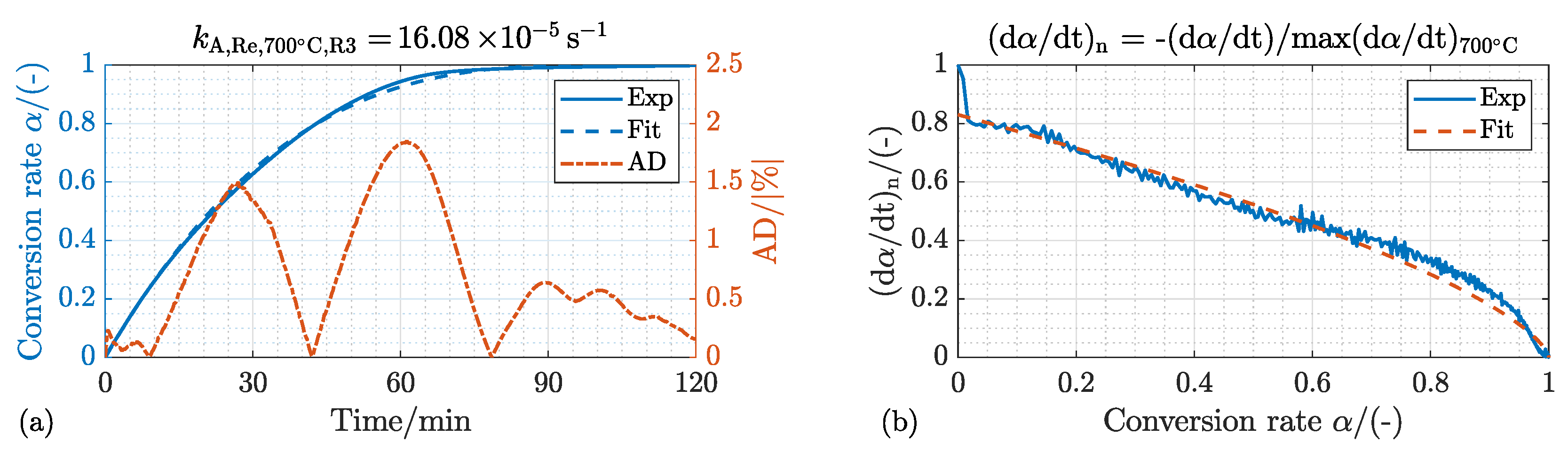
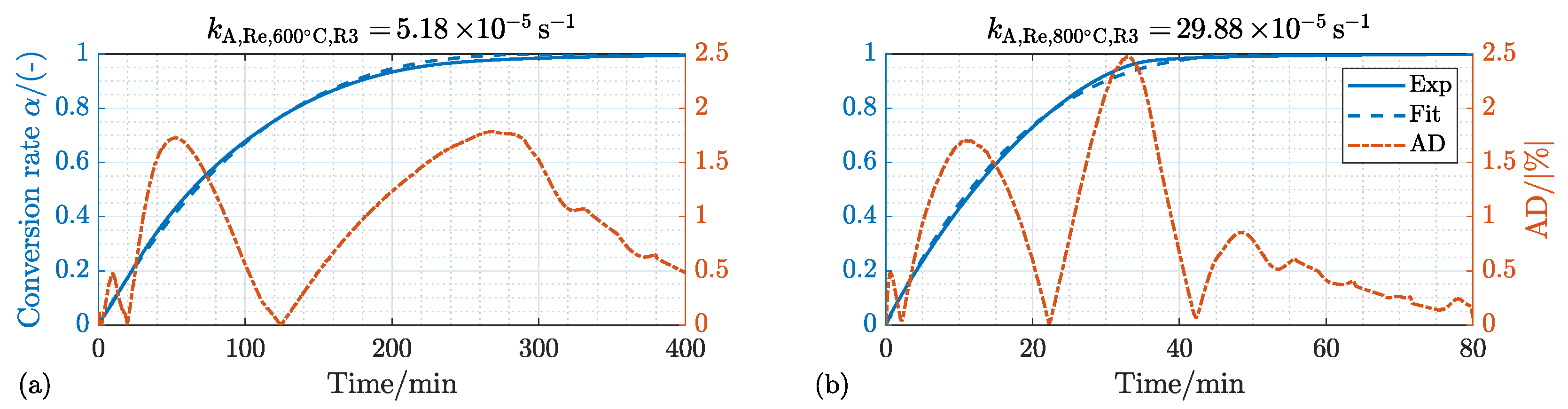
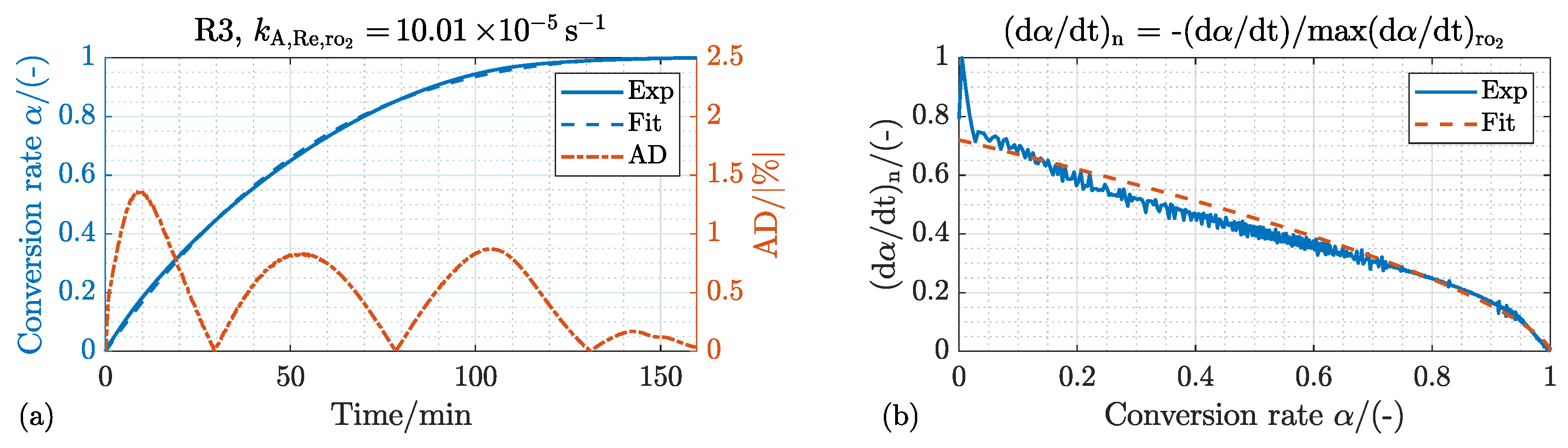
4.1.1. Kinetic Mechanism and Effect of the Process Temperature

As shown in Figure 5, the first step towards the estimation of the kinetic parameters is the selection of the kinetic mechansim from Table 1. To this aim, the experimental data have been normalised and plotted as shown in Figure 7, showing the isothermal reduction curves for 600   ° C , 700   ° C and 800   ° C over time (Figure 7a) and the time derivative of the reduction fractions over the reduction fraction (Figure 7b) of the sample mass. The presented results in Figure 7 belong exemplarily to the reactant gas concentration ro 3 according to Table 4.
Increasing the reaction temperature of the sample from 600 to 700   ° C results in a decrease in the time needed for the reduction fraction to reach α Re = 0.8 from 134 to 43   min (68%). Increasing the temperature further to 800   ° C results in an additional acceleration of the reduction reaction by 47% (from 43 to 23   min ). It can be concluded that the reduction reaction becomes faster with increasing the reaction temperature, which is common for such an endothermic reaction [45,83,84]. Furthermore, the curves in Figure 7b show a decelerating behavior, which indicates a phase boundary controlled reaction model. The high gradient, at the beginning, can be attributed to a short-term dominant surface diffusion, as illustrated in Figure 3 (Deceleratory).
First assumption from the graphical interpretation of Figure 7b can be confirmed by comparing the relevant reaction mechanism model from Table 1 in Figure 8. With the geometrical contracting sphere model R3 (see Figure 8c), the discrepancy between measured to fitted curves at a reactant flow rate of 250   mL/min with gas concentration ro 3 (see Table 4) and reaction temperature of 700   ° C amounts to AD Re , 700   ° C , R 3 ≤ 1.9%. Furthermore, the AD upon applying the A1.5 model decreases to less than AD Re , 700   ° C , A 1.5 < 1% from 56   min and a conversion degree of α > 0.919 . This result might indicate that nucleation growth can be the dominating process from this point on. As the conversion rate is already quite high, such an effect might not be important for a later practical application. However, from the scientific point of view, more dedicated investigations are needed to find out whether a hybridisation between different models might be leading to a much higher modelling accuracy. In addition, the model R2 reveals also a moderate deviation from AD Re , 700   ° C , R 2 2.4% over the reaction time. Applying the other reaction models F1, A1.5 (Time 56   min ) and D3 results in remarkably increased deviations between experimental and theoretical curves as depicted in Figure 8.
In addition, an examination of the time derivative of the reduction fraction over the reduction fraction in Figure 9b also shows, above a conversion rate of α = 0.05 , a maximum deviation of AD Re , 700   ° C , R 3 5 % , which proves that R3 or the geometrical contracting sphere model is perfectly suitable to describe the experimentally obtained hydrogen reduction kinetics at 700   ° C .
Figure 9 and Figure 10 confirm the excellent suitability of the reaction mechanism model R3 also for reaction temperatures 600   ° C and 800   ° C . With the model R3, the difference between the experimental curves and the fitted ones amounts to AD Re , 600   ° C , R 3 < 2% and AD Re , 800   ° C , R 3 < 2.5%.

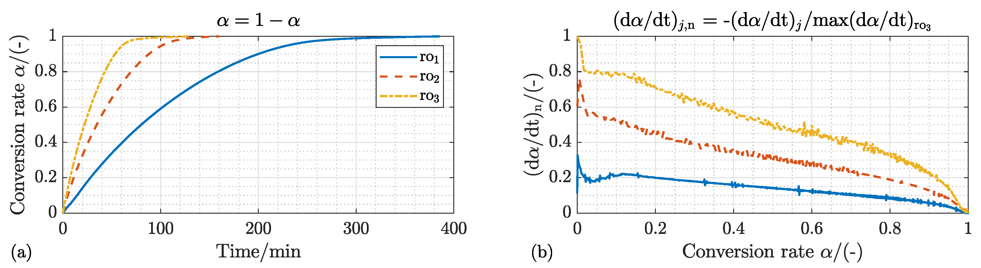
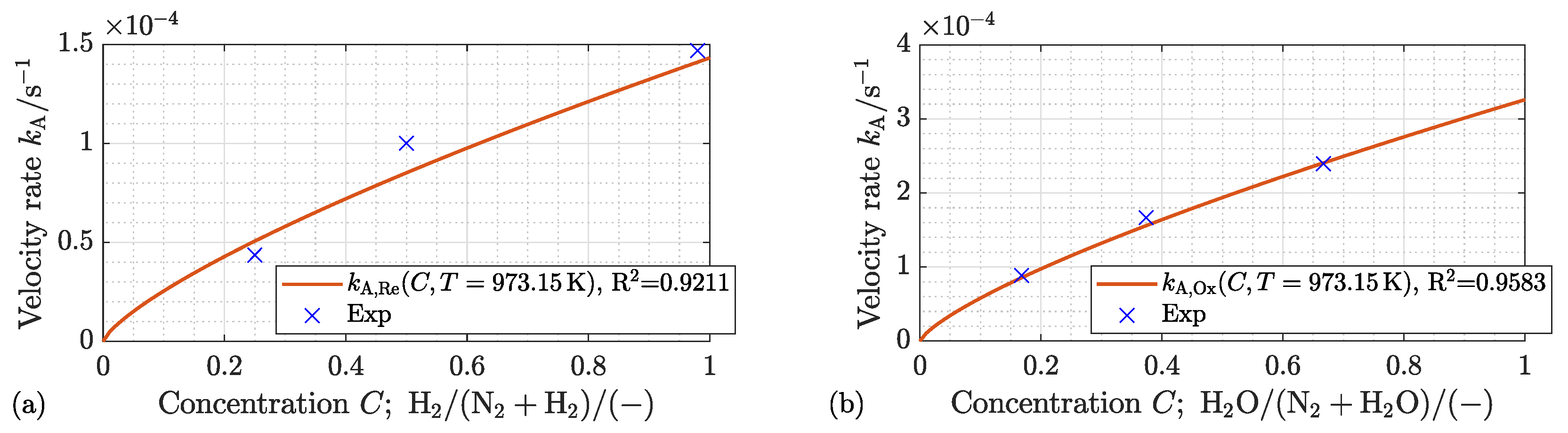
4.1.2. Effect of the Process Gas Composition

Figure 11a depicts the relative reduction fractions of the investigated pellet with different H2/N2 concentrations (cf. Table 4) at 700   ° C . The time needed to achieve a reduction of 80% of the maximum possible mass change ( α Re = 0.8 ) decreases to less than 72%, from 160   min down to 45   min as the H2 concentration in the reactive gas mixture increases from ro 1 to ro 3 . This is also confirmed by the study of [84]. Furthermore, the time derivative of the reduction fraction over the reduction fraction in Figure 11b shows the same decelerating behavior as Figure 11a, confirming the most suitability of a geometric contraction model.
Applying the geometrical contracting model R3 (see Figure 12a), the deviation between measured and fitted curves with gas concentration ro 2 and reaction temperature of 700   ° C amounts to AD Re , ro 2 , R 3 1.4%.
The investigation of temporal change in the reduction fraction over the reduction fraction in Figure 12b also shows a very good agreement between measured and calculated data. From a conversion rate of α = 0.05 , the discrepancy is AD Re , ro 2 , R 3 5%.
Figure 13 confirms the very good fit of the reaction mechanism model R3 to describe the experimental reduction kinetic data for gas concentration ro 1 –ro 3 together with Figure 12. With the model R3, the difference between the experimental curves and the fitted ones amounts to AD Re , ro 1 , R 3 < 1.3% and AD Re , ro 3 , R 3 < 1.9%. The optimised rate constants k A , n of Equation (40) for the R3 model are given on the top line of Figure 12a and Figure 13. It can be concluded that the higher the gas concentration, the higher the reduction rate constant k A , Re .

4.2. Oxidation

In contrast to the reduction reaction, there exist considerably less studies in the literature on the steam oxidation of iron for hydrogen production (see Table 5). This is mainly due to the fact that a large number of iron oxide reduction studies concentrate on the reduction of iron oxide in iron production processes. However, in the last few years, the number of publications dealing with hydrogen production by means of iron oxidation has increased [57,59,81,82]. Most of these research articles assumed that the oxidation is controlled by diffusion through the oxide layer, which is described by the diffusion model D3 (see Table 1). Kang [59], on the other hand, has shown that the control mechanism of the oxidation reaction can be determined by the chemical reaction at the interface (R3) upon studying a powdered calcined Fe2O3-20%ZrO2 sample.
In general, the oxidation of iron is the reversible process of Equations (2), (43) and (44). If the reaction temperature is above 576   ° C (the eutectoid point of the Fe-O system, see Figure 6), multilayer growth from pure iron to wuestite to magnetite takes place. Below 576   ° C , the wuestite phase is unstable, and the oxidation of iron produces directly magnetite, as already described for the reduction reaction in Section 4.1. For a detailed description of the individual oxidation steps and the associated valence ion migration, references [85,86] are highly recommended.
In addition, for the oxidation reaction, a relatively wide range for the oxidation activation energy (from 11 to 77.9   kJ/mol ) exist in the literature as presented in the lower part of Table 5. In order to have a precise simulation model for subsequent research tasks with the investigated storage material, a set of isothermal oxidation experiments was conducted at temperatures 600   ° C , 700   ° C and 800   ° C . In addition, the reacting gas concentration have been varied from ro 1 to ro 3 during the test campaign (see Table 4).

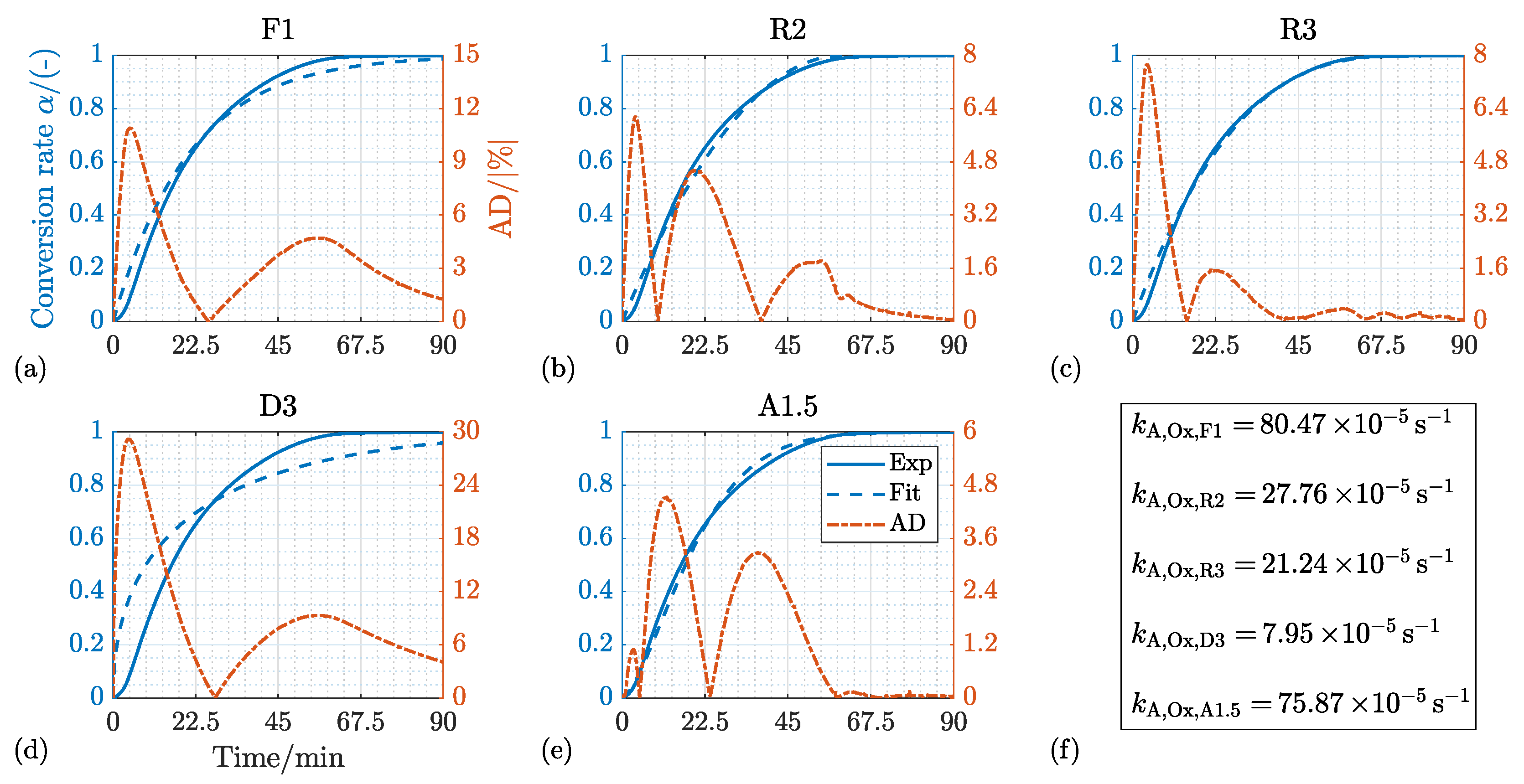
4.2.1. Kinetic Mechanism and Effect of the Process Temperature

As before, the kinetic mechanism formalism must be defined first in order to subsequently determine the kinetic parameters. For this purpose, the measured oxidation reaction data were normalised and plotted as shown in Figure 14. Here, the experimentally measured isothermal oxidation curves for 600   ° C , 700   ° C and 800   ° C over time are plotted (Figure 14a) and the time derivative of the oxidation fractions over time versus oxidation fraction (Figure 14b) for the reactant gas concentration ro 3 are shown in Table 4.
The curves in Figure 14a demonstrate an acceleration of the kinetic rate with the increase of the reaction temperature, which is a similiar result to those reported in [57,82]. Increasing the temperature of the sample from 600 to 700   ° C leads to a reduction in the time needed for the oxidation fraction to reach α Ox = 0.8 from 41 to 35   min (15%). Increasing the temperature further to 800   ° C leads to an additional acceleration of the oxidation reaction by 16% (time needed to reach a normalised conversion rate of 80% decreases from 32 to 27   min ).
Furthermore, the derivation of the measured curves represented in Figure 14b show an initial sigmoidal behavior between α Ox = 0 and α Ox = 0.18 . After attaining a maximum value, a deceleratory shape is observable, which indicates a phase boundary controlled reaction model (see Figure 3).
Different reaction mechanism models out of Table 1, namely, F1, R2, R3, D3 and A1.5, have been tested on their suitability to correlate the measured oxidation kinetic data, and the results are depicted in Figure 15. The presented curves belong to the isothermal oxidation temperature of 700   ° C and the reactant flow rate of 250   mL/min at the gas concentration ro 3 (see Table 4).
Sigmoidal behavior up to α Ox = 0.18 indicates a nucleation model, which is also consistent with the small deviation from AD Ox , 700   ° C , A 1.5 1% of the Avrami model A1.5 in Figure 15e. The deceleratory slope from α Ox = 0.18 to α Ox = 1 is again most accurately represented by the geometrical contracting model R3 in Figure 15c. Here, the deviation between measured and fitted amounts to AD Ox , 700   ° C , R 3 1.8%. Other models, such as reaction-based model F1 (Figure 15a) showed a deviation in the range AD Ox , 700   ° C , F 1 < 11%. The geometrical contracting model R2 (Figure 15b) is associated with a deviation in the range of AD Ox , 700   ° C , R 2 < 6%. The worst correlation results have been obtained upon applying the diffusion model D3 (Figure 15d) showing a deviation of AD Ox , 700   ° C , D 3 30%. In Figure 15f, the optimised rate constants k A , n of Equation (40) for all the tested reaction mechanism models are presented.
Figure 16 demonstrates the very good fitting of the reaction mechanism model R3 to correlate the experimental oxidation kinetic data at the temperatures 600   ° C , 700   ° C and 800   ° C . The correlation has been carried out above the conversion rate of α Ox > 0.01 , which adjusts k A , Ox , n . A detailed explanation for the reason behind this truncation is given in the next subsection. The deviation between the experimental curves and the fitted ones is AD Ox , 600   ° C , R 3 < 3.2%, AD Ox , 700   ° C , R 3 < 2.0% and AD Ox , 800   ° C , R 3 1.2%.

4.2.2. Effect of the Process Gas Composition

Figure 17a illustrates the oxidation conversion rates of the investigated pellet with different H2O/N2 concentrations (cf. Table 4) at 700   ° C . The time needed to achieve a conversion rate of α Ox = 0.8 decreases to less than 66% from 82   min down to 28   min as the H2O concentration in the reactive gas mixture increases from ro 1 to ro 3 .
Furthermore, the time derivatives of the oxidation fractions over the oxidation fraction in Figure 17b exhibit a non-consistent course in the range of α Ox 0.13 . For this purpose, the additional extract in Figure 17a is presented. It is obvious that a changing course of the temporal conversion rate variation exists for the operating condition ro 3 , if compared with the other two operating conditions (ro 1 and ro 2 ), over the first 5.5   min . Since the cubic starting slope of the conversion rate changes to a linear behavior with falling concentration, it is assumed that the non-consistency of ro 3 , at the begining, appears because of the dead time between the switchover of the MFC from pure N2 flow for the inertisation of the measuring cell to the flow time point of the H2O/N2 mixture. The steam generator needs, obviously, a couple of minutes until a continuous steam mass flow can be realised. The subsequent slope ( α Ox > 0.18 ) indicates a decelerating behavior as shown in Figure 14b, confirming the geometric contraction model. For the fitting purpose, the truncation of the data before ( α = 0.01 ) for this operating condition was enough to obtain a very good consistency with the other operating conditions.
Using the geometric contraction model R3 (see Figure 18), the maximum deviation between measured and fitted values at a reaction temperature of 700   ° C is AD Ox , j 2.7% (AD Ox , ro 1 , R 3 2.7%, AD Ox , ro 2 , R 3 1.8%, AD Ox , ro 3 , R 3 2%). Therefore, the functionality of the reaction mechanism model R3 for gas concentration ro 1 –ro 3 is confirmed. Furthermore, the higher the gas concentration, the higher the oxidation rate k A , Ox , n , as depicted on the header line of each separate figure.

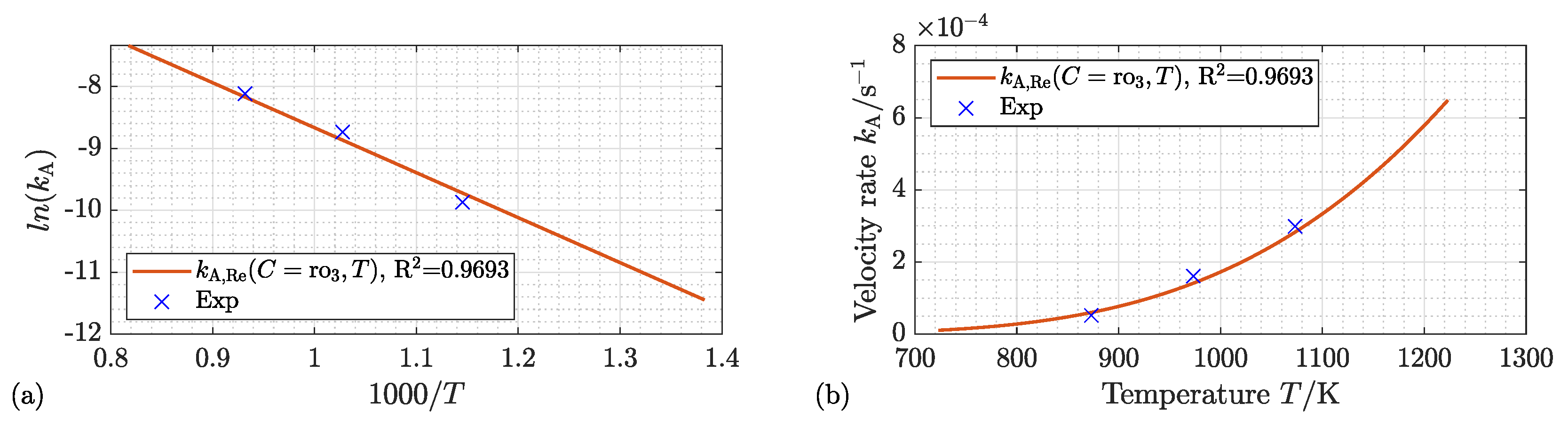
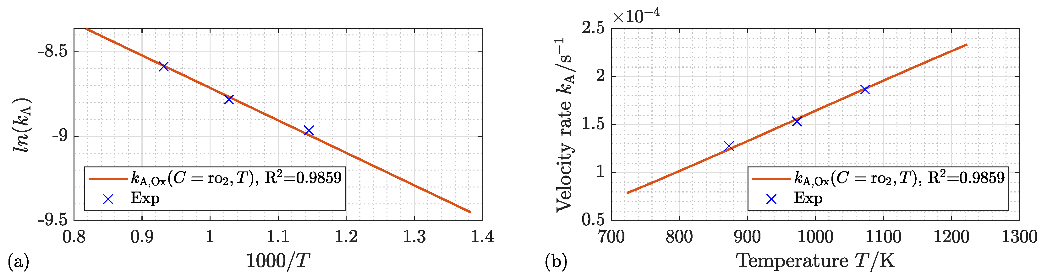
4.3. Activation Energy and Kinetic Velocity Rate

For developing a precise thermal management system of a redox reactor in the following development steps, the activation energy shall be described as accurately as possible as a function of its influencing parameters. Among other parameters, the activation energy E a depends on the chemical composition of the solid material, its physical properties and process temperature. All these parameters have an influence on the rate-limiting step, and therefore, different rate-limiting steps lead to different activation energies. The estimated values of the activation energy related to the hydrogen reduction of iron oxides and steam oxidation of iron in various studies are listed in Table 5. Indeed, the listed values for the activation energy exhibit a wide range for the reduction reaction, from 36 to 200   kJ/mol , as well as for the oxidation reaction, 11 to 77.9   kJ/mol . In addition, E a for both reactions, reduction and oxidation, decreases with increasing the temperature. The oxidation process shows also a higher reactivity with increasing the steam concentration.
It can, therefore, be concluded that the activation energy cannot be selected from the literature unless the material and the operating conditions are exactly similar. In other words, for the introduced iron oxide pellet in this work, the activation energy shall be described as a function of its influencing parameters based on the obtained experimental kinetic data. One of the most common methodologies to describe the activation energy is its formulation as an Arrhenius equation. Arrhenius published the followed equation in the year 1889 based on empirical considerations for the calculation of the activation energy [87]:
k A = A e E a R T
The temperature dependency is given by the exponential term and the pre-exponential factor A is a constant. It is possible to determine the activation energy from a series of kinetic measurements by plotting the logarithm of the rate constant against the reciprocal of the absolute temperature, as shown by the transformation of the Equation (35) to
ln ( k A ) = ln ( A ) E a R 1 T
The slope of such a straight line is proportional to the activation energy and the intercept to the pre-factor (A). The following equation can be simply derived from the past equation to estimate the activation energy.
E a = R ln ( k A ) ( 1 / T ) = R T 2 ln ( k A ) T
Combined with Equation (41), the activation energy graphs for the reduction reaction (see Figure 19) and the oxidation reaction (see Figure 20) were calculated. Figure 19a and Figure 20a illustrate the linearised descriptions according to Equation (46) for the reduction and oxidation reactions, respectively, while Figure 19b and Figure 20b depict the general Arrhenius form according to Equation (45). From the slopes of the linearised graphs, the activation energy for reduction is estimated to E a , Re = 56,858 J/mol and for oxidation to E a , Ox = 16,001 J/mol. The estimated E a values can be utilised to describe the temperature-dependency of the rate constant for both reduction and oxidation with a coefficient of determination of R 2 = 0.98336 and R 2 = 0.9858 , respectively.
Compared to reduction, the temperature has a 71% smaller effect on the reaction kinetics of oxidation. This is attributed to the lower activation energy of oxidation. Furthermore, both reaction rates increase with increasing the temperature. In terms of the reduction reaction, the obtained temperature dependency is consistent with the endothermic reaction mechanism. On the other hand, the temperature dependency of the oxidation reaction is traced back to the fact that enhanced diffusion processes have a larger impact on the reaction rate than the inhibited exothermic reaction mechanism due to the higher temperatures.
In addition to the discussed temperature dependency of the velocity rate k A , the dependency on the reaction gas concentration C can also be described in the general Arrhenius equation. To this aim, the concentration C raised to an empirical exponent parameter n is added as a multiplier to the typical Arrhenius equation to describe both temperature and concentration of the respective reactive gas component in the gas phase on the reaction rate [58,59,60]:
k A ( C , T ) = A e E a R T C n
In combination with the calculated activation energies and the non-linear least square fitting methodology (see Figure 5), the parameter n was determined to be n = 0.75 for both reduction and oxidation. With a coefficient of determination of R 2 = 0.9211 and R 2 = 0.958 , Figure 21a,b illustrate a good accuracy with the determined parameter n for the concentration-dependent description of the velocity rate at, for instance, a reaction temperature of 700   ° C . Furthermore, according to Figure 21a,b, both reaction rates increase with increasing the concentration of the respective reactive gas. In case of oxidation, the incremental rate of change with rising concentration is almost twice as high as in the case of reduction. Indeed, more experimental runs are needed at other reacting gas concentrations and temperatures in order to further enhance the fitting accuracy ( R 2 ) of the model. This will be the subject of our near future activities and publications.
In summary, based on the parameters for E a , A, and n determined from the redox experiments described here, a temperature- and concentration-dependent description for the velocity rate constant can be expressed as follows:
k A , Re ( C , T ) = 0.1813   s 1 · C H 2 O , in 0.75 · e 56.9   kJ/mol R T
k A , Ox ( C , T ) = 0.0023   s 1 · C H 2 O , in 0.75 · e 16.0 kJ/mol R T
Figure 22a,b present the calculated velocity rate constants of Equations (49) and (50) as a function of temperature T and gas concentration C. Compared to oxidation, the temperature has a smaller effect on the velocity rate constant of reduction, which is due to the higher activation energy. This explains also the lower temperature gradients in Figure 22a compared to Figure 22b.
Based on the identified best-suited kinetic model (R3) and the estimated parameters E a , A, and n, the following expressions are suggested to describe the temperature- and concentration-dependent conversion rate of both reduction and oxidation reactions on the investigated iron oxide pellet:
d α Re ( C , T ) d t = 0.5439   s 1 · C H 2 O , in 0.75 · e 56.9   kJ/mol R T · ( 1 α ) 2 / 3
d α Ox ( C , T ) d t = 0.0069   s 1 · C H 2 O , in 0.75 · e 16.0   kJ/mol R T · ( 1 α ) 2 / 3

5. Conclusions

In this work, the kinetics of both reduction and oxidation (redox) reactions on an iron oxide/iron pellet have been experimentally investigated under different isothermal conditions and different concentrations of the respective reacting gas. In addition, a comprehensive literature review has been conducted on the existing kinetic models and their suitability to describe the obtained results. It can be concluded that the so-called shrinking core model is best suited to describe the measured kinetic data. Additionally, the literature review showed a wide range for the activation energies of both redox reactions. Furthermore, the reported kinetic parameters are quite sensitive to small changes in the sample structure as well as in the process parameters. For this reason, the kinetic mechanisms and the activation energy for the investigated storage material were determined under different reaction temperatures and process gas concentrations.
Furthermore, it turned out that by applying the geometrical contracting sphere reaction model (R3), both measured concentration- and temperature-dependent reduction and oxidation rates could be reproduced analytically with a maximum deviation of less than 5%. Higher concentrations of the relevant reactive gas component within the input gas stream as well as elevated temperatures resulted in an accelerated conversion and, accordingly, a shorter time period to accomplish the reaction. Compared to the oxidation reaction, the temperature showed a greater effect on the reduction kinetics, which is attributed to the higher reduction activation energy ( E a , Re = 56.9   kJ/mol versus E a , Ox = 16.0   kJ/mol ). Oxidation showed, however, a nearly twofold increase in the reaction rate constant with increasing concentration if compared to the reduction reaction.
With the estimated activation energies, the temperature dependency of the rate constants for both reduction and oxidation could be very well described with an Arrhenius equation with a coefficient of determination of R 2 = 0.98336 and R 2 = 0.9858 , respectively. To describe the concentration C dependence of the rate constants, an empirical exponent has been introduced and estimated to n = 0.75 , with which the velocity rate k A can be well described with a coefficient of determination for the reduction of R 2 = 0.913 and for the oxidation of R 2 = 0.958 .
The obtained results pave the way to implement the obtained correlations to model both isothermal and non-isothermal behaviours of single- and multi-pellet redox reactors for designing and optimising the hydrogen storage process. These development results will be the subject of our next research.

Author Contributions

Conceptualisation, B.G. and B.D.; methodology, B.G. and B.D.; software, B.G.; validation, B.G. and L.H.; formal analysis, B.G. and B.D.; investigation, B.G.; resources, B.G. and B.D.; data curation, B.G. and B.D.; writing—original draft preparation, B.G.; writing—review and editing, B.G., L.H., M.G. and B.D.; visualisation, B.G.; supervision, M.G. and B.D. All authors have read and agreed to the published version of the manuscript.

Funding

The authors would like to acknowledge the project funding by the German Federal Ministries of Education and Research (BMBF) and Economics and Energy (BMWi), Project Number 03SBE113D.

Data Availability Statement

The data presented in this study are available on request from the first author.

Acknowledgments

The first author would like to acknowledge the support of the Regensburg Center of Energy and Resources (RCER) of OTH Regensburg, the Technology and Science Network Oberpfalz (TWO) and the BayWISS Joint Academic Partnership “Energy”.

Conflicts of Interest

The authors declare no conflict of interest.

References

  1. US National Aeronautics and Space - Climate Change Evidence: How Do We Know? Global Climate Change Vital Signs of the Planet. Available online: https://climate.nasa.gov/evidence/ (accessed on 2 October 2022).
  2. International Renewable Energy Agency. Global Renewables Outlook: Energy Transformation 2050; International Renewable Energy Agency: Abu Dhabi, United Arab Emirates, 2020. [Google Scholar]
  3. Thess, A.; Trieb, F.; Wörner, A.; Zunft, S. Herausforderung Wärmespeicher. Phys. J. 2015, 33–39. [Google Scholar]
  4. Sterner, M.; Stadler, I. Handbook of Energy Storage; Springer: Berlin/Heidelberg, Germany, 2019. [Google Scholar] [CrossRef]
  5. Klell, M.; Eichlseder, H.; Trattner, A. Wasserstoff in der Fahrzeugtechnik: Erzeugung Speicherung Anwendung, 4. aufl. 2018 ed.; ATZ/MTZ-Fachbuch; Springer: Wiesbaden, Germany, 2018. [Google Scholar]
  6. Lorente, E.; Peña, J.A.; Herguido, J. Cycle Behaviour of Iron Ores in the Steam-Iron Process. Int. J. Hydrogen Energy 2011, 36, 7043–7050. [Google Scholar] [CrossRef]
  7. Berger, C.M.; Mahmoud, A.; Hermann, R.P.; Braun, W.; Yazhenskikh, E.; Sohn, Y.J.; Menzler, N.H.; Guillon, O.; Bram, M. Calcium-Iron Oxide as Energy Storage Medium in Rechargeable Oxide Batteries. J. Am. Ceram. Soc. 2016, 99, 4083–4092. [Google Scholar] [CrossRef]
  8. Müller, K. Technologies for the Storage of Hydrogen Part 1: Hydrogen Storage in the Narrower Sense. Chem. Ing. Tech. 2019, 91, 383–392. [Google Scholar] [CrossRef]
  9. Voitic, G.; Hacker, V. Recent Advancements in Chemical Looping Water Splitting for the Production of Hydrogen. RSC Adv. 2016, 6, 98267–98296. [Google Scholar] [CrossRef] [Green Version]
  10. Hossain, M.M.; de Lasa, H.I. Chemical-Looping Combustion (CLC) for Inherent CO2 Separations—A Review. Chem. Eng. Sci. 2008, 63, 4433–4451. [Google Scholar] [CrossRef]
  11. Thaler, M.; Hacker, V. Storage and Separation of Hydrogen with the Metal Steam Process. Int. J. Hydrogen Energy 2012, 37, 2800–2806. [Google Scholar] [CrossRef]
  12. Lane, H. Apparatus for Producing Hydrogen Gas. U.S. Patent 1,028,366, 4 June 1912. [Google Scholar]
  13. Messerschmitt, A. Process of Producing Hydrogen. U.S. Patent 971,206, 27 September 1910. [Google Scholar]
  14. Heidari, A.; Niknahad, N.; Iljana, M.; Fabritius, T. A Review on the Kinetics of Iron Ore Reduction by Hydrogen. Materials 2021, 14, 7540. [Google Scholar] [CrossRef]
  15. Spreitzer, D.; Schenk, J. Reduction of Iron Oxides with Hydrogen—A Review. Steel Res. Int. 2019, 90, 1900108. [Google Scholar] [CrossRef] [Green Version]
  16. Feilmayr, C.; Thurnhofer, A.; Winter, F.; Mali, H.; Schenk, J. Reduction Behavior of Hematite to Magnetite under Fluidized Bed Conditions. ISIJ Int. 2004, 44, 1125–1133. [Google Scholar] [CrossRef] [Green Version]
  17. Levenspiel, O. Chemical Reaction Engineering, 3rd ed.; Wiley: New York, NY, USA, 1999. [Google Scholar]
  18. Gamisch, B.; Gaderer, M.; Dawoud, B. On the Development of Thermochemical Hydrogen Storage: An Experimental Study of the Kinetics of the Redox Reactions under Different Operating Conditions. Appl. Sci. 2021, 11, 1623. [Google Scholar] [CrossRef]
  19. Jin, X.; Zhao, X.; White, R.E.; Huang, K. Heat Balance in a Planar Solid Oxide Iron-Air Redox Battery: A Computational Analysis. J. Electrochem. Soc. 2015, 162, F821–F833. [Google Scholar] [CrossRef] [Green Version]
  20. Braun, W.; Erfurt, V.; Thaler, F.; Menzler, N.H.; Spatschek, R.; Singheiser, L. Kinetic Study of Iron Based Storage Materials for the Use in Rechargeable Oxide Batteries (ROB). ECS Trans. 2017, 75, 59–73. [Google Scholar] [CrossRef]
  21. Berger, C.M.; Tokariev, O.; Orzessek, P.; Hospach, A.; Fang, Q.; Bram, M.; Quadakkers, W.J.; Menzler, N.H.; Buchkremer, H.P. Development of Storage Materials for High-Temperature Rechargeable Oxide Batteries. J. Energy Storage 2015, 1, 54–64. [Google Scholar] [CrossRef]
  22. Bock, S.; Zacharias, R.; Hacker, V. High Purity Hydrogen Production with a 10 kWth RESC Prototype System. Energy Convers. Manag. 2018, 172, 418–427. [Google Scholar] [CrossRef]
  23. Zacharias, R.; Visentin, S.; Bock, S.; Hacker, V. High-Pressure Hydrogen Production with Inherent Sequestration of a Pure Carbon Dioxide Stream via Fixed Bed Chemical Looping. Int. J. Hydrogen Energy 2019, 44, 7943–7957. [Google Scholar] [CrossRef]
  24. Otsuka, K.; Yamada, C.; Kaburagi, T.; Takenaka, S. Hydrogen Storage and Production by redox of Iron Oxide for Polymer Electrolyte Fuel Cell Vehicles. Int. J. Hydrogen Energy 2003, 28, 335–342. [Google Scholar] [CrossRef]
  25. Takenaka, S.; Nomura, K.; Hanaizumi, N.; Otsuka, K. Storage and Formation of pure Hydrogen mediated by the redox of modified Iron Oxides. Appl. Catal. A Gen. 2005, 282, 333–341. [Google Scholar] [CrossRef]
  26. Rusman, N.; Dahari, M. A Review on the Current Progress of Metal Hydrides Material for Solid-State Hydrogen Storage Applications. Int. J. Hydrogen Energy 2016, 41, 12108–12126. [Google Scholar] [CrossRef]
  27. Müller, K. Technologies for the Storage of Hydrogen Part 2: Irreversible Conversion and Comparison. Chem. Ing. Tech. 2019, 91, 393–402. [Google Scholar] [CrossRef]
  28. Williams, P.T. Pyrolysis of Waste Tyres: A Review. Waste Manag. 2013, 33, 1714–1728. [Google Scholar] [CrossRef] [PubMed] [Green Version]
  29. Posdziech, O.; Schwarze, K.; Brabandt, J. Efficient Hydrogen Production for Industry and Electricity Storage via High-Temperature Electrolysis. Int. J. Hydrogen Energy 2019, 44, 19089–19101. [Google Scholar] [CrossRef]
  30. Betsch, K.; Knauf, G.; Kobow, C.; Martin, H.; Petzold, D.; Ufer, J.; Wolf, B. Verfahren zur Erzeugung von Wasserstoff oder Wasserstoffreichen Gasen. DD 000,000,094,984, 1 March 1972. [Google Scholar]
  31. Ertl, G. Handbook of Heterogeneous Catalysis, 2nd, completely rev. and enl. ed.; WILEY-VCH: Weinheim, Germany; Chichester, UK, 2008. [Google Scholar]
  32. Engell, H.J.; von Bogdandy, L. (Eds.) Die Reduktion der Eisenerze: Wissenschaftliche Grundlagen und Technische Durchführung; Springer: Berlin/Heidelberg, Germany, 1967. [Google Scholar] [CrossRef]
  33. Ebrahimi, A.A.; Ebrahim, H.A.; Hatam, M.; Jamshidi, E. Finite Element Solution for Gas–Solid Reactions: Application to the Moving Boundary Problems. Chem. Eng. J. 2008, 144, 110–118. [Google Scholar] [CrossRef]
  34. Szekely, J.; Evans, J.W.; Sohn, H.Y. Gas-Solid Reactions; Academic Press: New York, NY, USA, 1976. [Google Scholar]
  35. Kim, S.H.; Zhang, X.; Ma, Y.; Souza Filho, I.R.; Schweinar, K.; Angenendt, K.; Vogel, D.; Stephenson, L.T.; El-Zoka, A.A.; Mianroodi, J.R.; et al. Influence of Microstructure and Atomic-Scale Chemistry on the Direct Reduction of Iron Ore with Hydrogen at 700 °C. Acta Mater. 2021, 212, 116933. [Google Scholar] [CrossRef]
  36. Emig, G.; Klemm, E. Chemische Reaktionstechnik; Springer: Berlin/Heidelberg, Germany, 2017. [Google Scholar] [CrossRef]
  37. Chorkendorff, I.; Niemantsverdriet, J.W. Concepts of Modern Catalysis and Kinetics; Wiley: Hoboken, NJ, USA, 2003. [Google Scholar] [CrossRef]
  38. Gómez-Barea, A.; Ollero, P. An approximate Method for solving Gas–Solid Non-Catalytic Reactions. Chem. Eng. Sci. 2006, 61, 3725–3735. [Google Scholar] [CrossRef]
  39. Melchiori, T.; Canu, P. Improving the Quantitative Description of Reacting Porous Solids: Critical Analysis of the Shrinking Core Model by Comparison to the Generalized Grain Model. Ind. Eng. Chem. Res. 2014, 53, 8980–8995. [Google Scholar] [CrossRef]
  40. Khawam, A.; Flanagan, D.R. Solid-State Kinetic Models: Basics and Mathematical Fundamentals. J. Phys. Chem. B 2006, 110, 17315–17328. [Google Scholar] [CrossRef]
  41. Khawam, A.; Flanagan, D.R. Basics and Applications of Solid-State Kinetics: A Pharmaceutical Perspective. J. Pharm. Sci. 2006, 95, 472–498. [Google Scholar] [CrossRef]
  42. Li, Q.; Lin, X.; Luo, Q.; Chen, Y.; Wang, J.; Jiang, B.; Pan, F. Kinetics of the Hydrogen Absorption and Desorption Processes of Hydrogen Storage Alloys: A Review. Int. J. Miner. Metall. Mater. 2022, 29, 32–48. [Google Scholar] [CrossRef]
  43. Pang, Y.; Li, Q. A Review on Kinetic Models and Corresponding Analysis Methods for Hydrogen Storage Materials. Int. J. Hydrogen Energy 2016, 41, 18072–18087. [Google Scholar] [CrossRef]
  44. Faraji, F.; Alizadeh, A.; Rashchi, F.; Mostoufi, N. Kinetics of Leaching: A Review. Rev. Chem. Eng. 2022, 38, 113–148. [Google Scholar] [CrossRef]
  45. El-Geassy, A.A. Gaseous Reduction of Fe2O3 Compacts at 600 to 1050 °C. J. Mater. Sci. 1986, 21, 3889–3900. [Google Scholar] [CrossRef]
  46. Parisi, D.R.; Laborde, M.A. Modeling of Counter Current Moving Bed Gas-Solid Reactor Used in Direct Reduction of Iron Ore. Chem. Eng. J. 2004, 104, 35–43. [Google Scholar] [CrossRef] [Green Version]
  47. Pineau, A.; Kanari, N.; Gaballah, I. Kinetics of Reduction of Iron Oxides by H2: Part I: Low temperature reduction of hematite. Thermochim. Acta 2006, 447, 89–100. [Google Scholar] [CrossRef]
  48. Turkdogan, E.T.; Vinters, J.V. Gaseous Reduction of Iron Oxides: Part I. Reduction of Hematite in Hydrogen. Metall. Mater. Trans. B 1971, 2, 3175–3188. [Google Scholar] [CrossRef]
  49. Usui, T.; Ohmi, M.; Yamamura, E. Analysis of Rate of Hydrogen Reduction of Porous Wustite Pellets Basing on Zone-Reaction Models. ISIJ Int. 1990, 30, 347–355. [Google Scholar] [CrossRef]
  50. King, P.L.; Wheeler, V.M.; Renggli, C.J.; Palm, A.B.; Wilson, S.A.; Harrison, A.L.; Morgan, B.; Nekvasil, H.; Troitzsch, U.; Mernagh, T.; et al. Gas–Solid Reactions: Theory, Experiments and Case Studies Relevant to Earth and Planetary Processes. Rev. Mineral. Geochem. 2018, 84, 1–56. [Google Scholar] [CrossRef]
  51. Szekely, J.; Evans, J.W. A Structural Model for Gas-Solid Reactions with a Moving Boundary-II. Chem. Eng. Sci. 1971, 26, 1901–1913. [Google Scholar] [CrossRef]
  52. Schüth, F. Handbook of Porous Solids; WILEY-VCH: Weinheim, Germany, 2002. [Google Scholar] [CrossRef]
  53. Valipour, M.S.; Motamed Hashemi, M.Y.; Saboohi, Y. Mathematical Modeling of the Reaction in an Iron Ore Pellet Using a Mixture of Hydrogen, Water Vapor, Carbon Monoxide and Carbon Dioxide: An Isothermal Study. Adv. Powder Technol. 2006, 17, 277–295. [Google Scholar] [CrossRef]
  54. Hossain, M.M.; de Lasa, H.I. Reduction and Oxidation Kinetics of Co–Ni/Al2O3 Oxygen Carrier Involved in a Chemical-Looping Combustion Cycles. Chem. Eng. Sci. 2010, 65, 98–106. [Google Scholar] [CrossRef]
  55. Piotrowski, K.; Mondal, K.; Wiltowski, T.; Dydo, P.; Rizeg, G. Topochemical Approach of Kinetics of the Reduction of Hematite to Wüstite. Chem. Eng. J. 2007, 131, 73–82. [Google Scholar] [CrossRef]
  56. Nouri, S.; Ale Ebrahim, H.; Jamshidi, E. Simulation of Direct Reduction Reactor by the Grain Model. Chem. Eng. J. 2011, 166, 704–709. [Google Scholar] [CrossRef]
  57. Jeong, M.H.; Lee, D.H.; Bae, J.W. Reduction and Oxidation Kinetics of Different Phases of Iron Oxides. Int. J. Hydrogen Energy 2015, 40, 2613–2620. [Google Scholar] [CrossRef]
  58. Vyazovkin, S.; Burnham, A.K.; Criado, J.M.; Pérez-Maqueda, L.A.; Popescu, C.; Sbirrazzuoli, N. ICTAC Kinetics Committee Recommendations for Performing Kinetic Computations on Thermal Analysis Data. Thermochim. Acta 2011, 520, 1–19. [Google Scholar] [CrossRef]
  59. Kang, K.S.; Kim, C.H.; Bae, K.K.; Cho, W.C.; Jeong, S.U.; Lee, Y.J.; Park, C.S. Reduction and Oxidation Properties of Fe2O3/ZrO2 Oxygen Carrier for Hydrogen Production. Chem. Eng. Res. Des. 2014, 92, 2584–2597. [Google Scholar] [CrossRef]
  60. Guo, D.; Hu, M.; Pu, C.; Xiao, B.; Hu, Z.; Liu, S.; Wang, X.; Zhu, X. Kinetics and Mechanisms of Direct Reduction of Iron Ore-Biomass Composite Pellets with Hydrogen Gas. Int. J. Hydrogen Energy 2015, 40, 4733–4740. [Google Scholar] [CrossRef]
  61. Alonso, E.; Pérez-Rábago, C. Isothermal and Non-Isothermal Kinetics of Metal Oxide Redox Reactions Performed in a Solar Furnace. In AIP Conference Proceedings; AIP Publishing LLC.: Melville, NY, USA, 2018; Volume 2033, p. 100002. [Google Scholar] [CrossRef]
  62. Luo, L.; Zhang, Z.; Li, C.; Nishu; He, F.; Zhang, X.; Cai, J. Insight into Master Plots Method for Kinetic Analysis of Lignocellulosic Biomass Pyrolysis. Energy 2021, 233, 121194. [Google Scholar] [CrossRef]
  63. Vyazovkin, S.; Dollimore, D. Linear and Nonlinear Procedures in Isoconversional Computations of the Activation Energy of Nonisothermal Reactions in Solids. J. Chem. Inf. Comput. Sci. 1996, 36, 42–45. [Google Scholar] [CrossRef]
  64. Šesták, J.; Berggren, G. Study of the Kinetics of the Mechanism of Solid-State Reactions at Increasing Temperatures. Thermochim. Acta 1971, 3, 1–12. [Google Scholar] [CrossRef]
  65. Pérez-Maqueda, L.A.; Criado, J.M.; Sanchez-Jiménez, P.E. Combined Kinetic Analysis of Solid-State Reactions: A Powerful Tool for the Simultaneous Determination of Kinetic Parameters and the Kinetic Model Without Previous Assumptions on the Reaction Mechanism. J. Phys. Chemistry. A 2006, 110, 12456–12462. [Google Scholar] [CrossRef]
  66. DIN EN 14647:2005; Calcium Aluminate Cement—Composition, Specifications and Conformity Criteria. Beuth Verlag GmbH: Berlin, Germany, 2007.
  67. Huber, L.; Gamisch, B.; Dawoud, B. Experimental Investigation of the Cycle Stability of Different Iron Oxide Composites for a Redox Hydrogen Storage Process. In Proceedings of the International Renewable Energy Storage Conference 2021 (IRES 2021), Paris, France, 18–22 November 2022. [Google Scholar] [CrossRef]
  68. Mehmood, T.; Liland, K.H.; Snipen, L.; Sæbø, S. A Review of Variable Selection Methods in Partial Least Squares Regression. Chemom. Intell. Lab. Syst. 2012, 118, 62–69. [Google Scholar] [CrossRef]
  69. Heumann, T. Diffusion in Metallen: Grundlagen Theorie Vorgänge in Reinmetallen und Legierungen; Springer: Berlin/Heidelberg, Germany, 1992; Volume 10. [Google Scholar]
  70. Piotrowski, K.; Mondal, K.; Lorethova, H.; Stonawski, L.; Szymanski, T.; Wiltowski, T. Effect of Gas Composition on the Kinetics of Iron Oxide Reduction in a Hydrogen Production Process. Int. J. Hydrogen Energy 2005, 30, 1543–1554. [Google Scholar] [CrossRef]
  71. Zhang, W.; Zhang, J.; Li, Q.; He, Y.; Tang, B.; Li, M.; Zhang, Z.; Zou, Z. Thermodynamic Analyses of Iron Oxides Redox Reactions. In Proceedings of the 8th Pacific Rim International Congress on Advanced Materials and Processing, Waikoloa, HI, USA, 4–9 August 2013; Marquis, F., Ed.; Springer International Publishing: Cham, Switzerland, 2016; Volume 44, pp. 777–789. [Google Scholar] [CrossRef]
  72. Takenaka, Y.; Kimura, Y.; Narita, K.; Kaneko, D. Mathematical Model of Direct Reduction Shaft Furnace and its Application to Actual Operations of a Model Plant. Comput. Chem. Eng. 1986, 10, 67–75. [Google Scholar] [CrossRef]
  73. Pineau, A.; Kanari, N.; Gaballah, I. Kinetics of Reduction of Iron Oxides by H2: Part II. Low temperature reduction of magnetite. Thermochim. Acta 2007, 456, 75–88. [Google Scholar] [CrossRef]
  74. El-Geassy, A.A.; Shehata, K.A.; Ezz, S.Y. Mechanism of Iron Oxide Reduction with Hydrogen/Carbon Monoxide Mixtures. Trans. Iron Steel Inst. Jpn. 1977, 17, 629–635. [Google Scholar] [CrossRef] [Green Version]
  75. Lin, H.Y.; Chen, Y.W.; Li, C. The Mechanism of Reduction of Iron Oxide by Hydrogen. Thermochim. Acta 2003, 400, 61–67. [Google Scholar] [CrossRef]
  76. Manchili, S.K.; Wendel, J.; Hryha, E.; Nyborg, L. Analysis of Iron Oxide Reduction Kinetics in the Nanometric Scale Using Hydrogen. Nanomaterials 2020, 10, 1276. [Google Scholar] [CrossRef]
  77. Munteanu, G.; Ilieva, L.; Andreeva, D. TPR Data regarding the Effect of Sulfur on the Reducibility of Alpha-Fe2O3. Thermochim. Acta 1999, 329, 157–162. [Google Scholar] [CrossRef]
  78. Munteanu, G.; Ilieva, L.; Andreeva, D. Kinetic Parameters obtained from TPR Data for Alpha-Fe2O3 and Systems. Thermochim. Acta 1997, 291, 171–177. [Google Scholar] [CrossRef]
  79. Kuila, S.K.; Chatterjee, R.; Ghosh, D. Kinetics of Hydrogen Reduction of Magnetite Ore Fines. Int. J. Hydrogen Energy 2016, 41, 9256–9266. [Google Scholar] [CrossRef]
  80. Coetsee, T.; Pistorius, P.; de Villiers, E. Rate-Determining Steps for Reduction in Magnetite-Coal Pellets. Miner. Eng. 2002, 15, 919–929. [Google Scholar] [CrossRef]
  81. Wen, F.; Wang, H.; Tang, Z. Kinetic Study of the Redox Process of Iron Oxide for Hydrogen Production at Oxidation Step. Thermochim. Acta 2011, 520, 55–60. [Google Scholar] [CrossRef]
  82. Go, K.; Son, S.; Kim, S. Reaction Kinetics of Reduction and Oxidation of Metal Oxides for Hydrogen Production. Int. J. Hydrogen Energy 2008, 33, 5986–5995. [Google Scholar] [CrossRef]
  83. Tsay, Q.T.; Ray, W.H.; Szekely, J. The Modeling of Hematite Reduction with Hydrogen Plus Carbon Monoxide Mixtures: Part I. The Behavior of Single Pellets. AIChE J. 1976, 22, 1064–1072. [Google Scholar] [CrossRef]
  84. Beheshti, R.; Moosberg-Bustnes, J.; Kennedy, M.W.; Aune, R.E. Reduction of Commercial Hematite Pellet in Isothermal Fixed Bed—Experiments and Numerical Modelling. Ironmak. Steelmak. 2016, 43, 31–38. [Google Scholar] [CrossRef] [Green Version]
  85. Chen, Z.; Zeilstra, C.; van der Stel, J.; Sietsma, J.; Yang, Y. Reduction Mechanism of Fine Hematite Ore Particles in Suspension. Metall. Mater. Trans. B 2021, 52, 2239–2252. [Google Scholar] [CrossRef]
  86. Yu, X.; Ji, Z. Grain Boundary in Oxide Scale During High-Temperature Metal Processing. In Study of Grain Boundary Character; Tanski, T., Borek, W., Eds.; InTech: London, UK, 2017. [Google Scholar] [CrossRef] [Green Version]
  87. Laidler, K.J. The Development of the Arrhenius Equation. J. Chem. Educ. 1984, 61, 494. [Google Scholar] [CrossRef]
Figure 1. Schematic representation of the reduction process: (1) Diffusion of H2 through the macro pores; (2) Diffusion of H2 through the micro pores; (3) Chemical reaction; (4) Movement of the iron cations Fe n + and electrons e to the iron core; (5) Diffusion of H2O through micro pores; (6) Diffusion of H2O through macro pores (inspired by [32]).
Energies 15 08322 g001
Figure 2. Simplified visualisation of the reaction model for a heterogeneous, non-catalytic redox reaction (based on Equation (2)): (a) Progressive-conversion model (PCM); (b) Shrinking core model (SCM); (c) Grain model (GM).
Energies 15 08322 g002
Figure 3. Schematic shape of reaction rate d α /dt against conversion α for isothermal solid-state reaction models, inspired by [15,40].
Energies 15 08322 g003
Figure 4. (a) Flowchart for the experimental procedure; (b) TGA setup for the experimental investigation of the kinetics of the redox reactions.
Energies 15 08322 g004
Figure 5. Flowchart to determine the kinetic parameters.
Energies 15 08322 g005
Figure 6. Predominant areas for iron oxide H2 reduction reactions with the eutectoid temperature of 576   ° C (- -), based on [71].
Energies 15 08322 g006
Figure 7. Effect of the reaction temperature on the temporal reduction fractions (a) and temporal change of the reduction fractions over reduction fraction (b) of the sample at a reactant flow rate of 250   mL/min and the gas concentration ro 3 as defined in Table 4; T6 = reaction temperature 600   ° C , T7 = reaction temperature 700   ° C , T8 = reaction temperature 800   ° C .
Energies 15 08322 g007
Figure 8. Temporal reduction fraction of sample (Exp) at a reactant flow rate of 250   mL/min with gas concentration ro 3 (see Table 4) and reaction temperature of 700   ° C compared to reaction mechanism models (Fit) of Table 1 with its absolute deviation (AD); (a) First-order reaction; (b) Geometrical contracting cylinder; (c) Geometrical contracting sphere; (d) 3D Diffusion Jander eqn.; (e) Nucleation and growth model (n = 1.5); (f) Optimised rate constants of Equation (40) for the specific reaction mechanism models.
Energies 15 08322 g008
Figure 9. Reduction behavior of sample (Exp) at a reactant flow rate of 250   mL/min with gas concentration ro 3 (see Table 4) and reaction temperature of 700   ° C compared to reaction mechanism model R3 (Fit) (see Table 1) with its absolute deviation (AD); (a) Temporal reduction fractions, (b) Temporal change of the reduction fractions over reduction fraction.
Energies 15 08322 g009
Figure 10. Temporal reduction fraction of sample (Exp) at a reactant flow rate of 250   mL/min with gas concentration ro 3 (see Table 4) compared to reaction mechanism models R3 (Fit) of Table 1 with its absolute deviation (AD); (a) Reaction temperature of 600   ° C ; (b) Reaction temperature of 800   ° C .
Energies 15 08322 g010
Figure 11. Effect of the gas concentrations j on the temporal reduction fractions (a) and temporal change of the reduction fractions over reduction fraction (b) of the sample at a reactant flow rate of 250   mL/min and reaction temperature of 700   ° C ; ro 1 , ro 2 and ro 3 as defined in Table 4.
Energies 15 08322 g011
Figure 12. Reduction behavior of sample (Exp) at a reactant flow rate of 250   mL/min with gas concentration ro 2 (see Table 4) and reaction temperature of 700   ° C compared to reaction mechanism model R3 (Fit) (see Table 1) with its absolute deviation (AD); (a) Temporal reduction fractions; (b) Temporal change of the reduction fractions over reduction fraction.
Energies 15 08322 g012
Figure 13. Temporal reduction fraction of sample (Exp) at a reactant flow rate of 250   mL/min with a reaction temperature of 700   ° C compared to reaction mechanism models R3 (Fit) of Table 1 with its absolute deviation (AD); (a) Gas concentration of ro 1 ; (b) Gas concentration of ro 3 (see Table 4).
Energies 15 08322 g013
Figure 14. Effect of the reaction temperature on the temporal oxidation fractions (a) and temporal change of the oxidation fractions over oxidation fraction (b) of the sample at a reactant flow rate of 250   mL/min and the gas concentration ro 3 as defined in Table 4; T6 = reaction temperature 600   ° C , T7 = reaction temperature 700   ° C , T8 = reaction temperature 800   ° C .
Energies 15 08322 g014
Figure 15. Temporal oxidation fraction of sample (Exp) at a reactant flow rate of 250   mL/min with gas concentration ro 3 (see Table 4) and reaction temperature of 700   ° C compared to reaction mechanism models (Fit) of Table 1 with its absolute deviation (AD); (a) First-order reaction; (b) Geometrical contracting cylinder; (c) Geometrical contracting sphere; (d) 3D Diffusion Jander eqn.; (e) Nucleation and growth model (n = 1.5); (f) Optimised rate constants of Equation (34) for the specific reaction mechanism models.
Energies 15 08322 g015
Figure 16. Temporal oxidation fraction of sample (Exp) at a reactant flow rate of 250   mL/min with gas concentration ro 3 (see Table 4) compared to reaction mechanism models R3 (Fit) of Table 1 with its absolute deviation (AD); (a) Reaction temperature of 600   ° C ; (b) Reaction temperature of 700   ° C ; (c) Reaction temperature of 800   ° C .
Energies 15 08322 g016
Figure 17. Effect of the gas concentrations j = [ro 1 ,ro 2 ,ro 3 ] on the temporal oxidation fractions (a) and temporal change of the oxidation fractions over oxidation fraction (b) of the sample at a reactant flow rate of 250   mL/min and reaction temperature of 700   ° C ; ro 1 , ro 2 and ro 3 (see Table 4).
Energies 15 08322 g017
Figure 18. Temporal oxidation fraction of sample (Exp) at a reactant flow rate of 250   mL/min with a reaction temperature of 700   ° C compared to reaction mechanism models R3 (Fit) of Table 1 with its absolute deviation (AD); (a) Gas concentration of ro 1 ; (b) Gas concentration of ro 2 ; (c) Gas concentration of ro 3 (see Table 4).
Energies 15 08322 g018
Figure 19. Velocity rate for the reduction of sample (Exp) at a reactant flow rate of 250   mL/min with a gas concentration ro 3 at reaction temperature of 450 to 950   ° C compared to fitted model ( k A ); (a) In logarithmic form for the determination of the activation energy; (b) In the general Arrhenius form.
Energies 15 08322 g019
Figure 20. Velocity rate for the oxidation of sample (Exp) at a reactant flow rate of 250   mL/min with a gas concentration ro 2 at reaction temperature of 450 to 950   ° C compared to fitted model ( k A ); (a) In logarithmic form for the determination of the activation energy; (b) In the general Arrhenius form.
Energies 15 08322 g020
Figure 21. Velocity rate for the reduction (a) and oxidation (b) of sample (Exp) at a reactant flow rate of 250   mL/min with a reaction temperature of 700   ° C at gas concentration ro 1 –ro 3 (see Table 4) compared to fitted model ( k A ).
Energies 15 08322 g021
Figure 22. Calculated velocity rate for (a) reduction k A , Re ( C , T ) and (b) oxidation k A , Ox ( C , T ) of the sample mass as a function of gas concentration C and reaction temperature T.
Energies 15 08322 g022
Table 1. Algebraic expressions for f ( α ) and g ( α ) functions for different kinetic models [40,50,62].
Reaction MechanismSymbolKinetic Mechanism Function
Differential FormIntegral Form
f ( α ) = 1 k A d α dt g ( α ) = k A t
Nucleation models (Avarami–Erofe’ev)
Nucleation and growth, n = order of reactionAn n ( 1 α ) [ ln ( 1 α ) ] ( n 1 ) / n [ ln ( 1 α ) ] 1 / n
Phase boundary-controlled reaction
Geometrical contracting infinite slab (Film Diffusion control)R11 α
Geometrical contracting cylinder (Chemical reaction control)R2 2 ( 1 α ) 1 / 2 1 ( 1 α ) 1 / 2
Geometrical contracting sphere (Chemical reaction control)R3 3 ( 1 α ) 2 / 3 1 ( 1 α ) 1 / 3
Diffusion models
3D Diffusion Jander eqn.D3 3 ( 1 α ) 2 / 3 2 ( 1 ( 1 α ) 1 / 3 ) [ 1 ( 1 α ) 1 / 3 ] 2
Ginstling–Brounshtein (Ash Layer, Diffusion control)D4 3 2 ( 1 α ) 1 / 3 1 1 2 3 α ( 1 α ) 2 / 3
Reaction order-based models
First-orderF1 ( 1 α ) ln ( 1 α )
Second-orderF2 ( 1 α ) 2 [ 1 / ( 1 α ) ] 1
Table 2. Combination of o, m and p as well as a description to possible mechanistic models [64]; models marked in italics are not considered here.
ompIs Suitable for:
Phase boundary controlled reaction
Phase boundary-controlled reaction (R2, R3), Reaction order models (F1)
Mampel Equation (P2, P3), linear nucleation and diffusion models
Gingstling–Brounshtein (D4), 2D diffusion models
Nucleation, latter stages of linear growth of nuclei
Growth of nulcei (A1.5–A4)
Unjustified as yet
Any complicated case, unjustified as yet
Table 3. List of all measuring device accuracies for the experimental setup.
DevicePhysical UnitMeasurement Accuracy
STA 449-F3, NetzschMass35,000 mg ± 0.0001 mg
Temperature 1600   ° C ± 0.3   ° C
EL-FLOW, BronkhorstGas flow (H2, N2) 250   mL/min ± 0.5%
Steam generator DV2MK, ADROPMass flow (H2O) 25   g/h ± 1%
Table 4. Influx molar concentrations of the reducing and oxidation gas mixtures during the four redox experiments ro 1 to ro 3 .
LabelReductionOxidation
H2/N2H2O/N2
mL min / mL min mol%/mol% g h / mL min mol%/mol%
ro 1 63/18725/751.8/16216/84
ro 2 125/12550/503.6/12533/67
ro 3 245/598/25.8/6067/33
Table 5. Summary of researcher on the iron oxides reduction by hydrogen as well as oxidation by steam and the used kinetics models.
ReactionTemperatureConc.GeometryModel E a ExperimentRef.
Fe 3 O 4 Fe 1173   K H 2 / C O = 1.5 Pellet, d = 15.2   mm R3 75.4   kJ/mol Isothermal[53,72]
FeO Fe 1173   K H 2 / C O = 1.5 Pellet, d = 15.2   mm R3 117.2   kJ/mol Isothermal[53,72]
Fe 2 O 3 Fe
(Fe2O3-20% ZrO2)
1023–1173 K H 2 / Ar = 10 –25%Powder, m = 20   mg R3 59   kJ/mol Isothermal[59]
Fe 2 O 3 Fe 973–1173 K10% H 2 + 90% N 2 Powder, m = 13   mg A2 23.9   kJ/mol Isothermal[70]
Fe 3 O 4 Fe 610–877 K100% H 2 Powder, m = 100   mg    A2/A3 < 690   K R1 > 691   K    39– 88   kJ/mol Isothermal[47]
Fe 3 O 4 Fe 493–956 K10% H 2 + 90% N 2 Powder, m = 100   mg    A2/A3 < 688   K Rx > 691   K    36– 103   kJ/mol Isothermal[47]
Fe 3 O 4 Fe 473–723 K100% H 2 Powder, m = 100   mg R2/R3 200   kJ/mol Isothermal[73]
523–663 K100% H 2 Powder, m = 100   mg R2/R3 71   kJ/mol Isothermal[73]
>663 K100% H 2 Powder, m = 100   mg A2 44   kJ/mol Isothermal[73]
Fe 2 O 3 Fe 973–1373 K100% H 2 Cyl., dxh = 9.8 × 11.1   mm 2 - 53.5   kJ/mol Isothermal[74]
Fe 2 O 3 Fe 1123–1323 K100% H 2 Pellet, d = 10 15   mm R3 122   kJ/mol Isothermal[60]
Fe 3 O 4 Fe 603–1003 K5% H 2 / N 2 Powder, m = 10 15   mg A2 70.4   kJ/mol Nonisothermal[75]
Fe 3 O 4 Fe 703–953 K83% H 2 /ArPowder, m = 100   mg -45– 55   kJ/mol Nonisothermal[76]
Fe 3 O 4 Fe 600–1000 K10% H 2 /ArPowder, m = 100   mg -   93.2– 103   kJ/mol       Nonisothermal   [77]
Fe 3 O 4 FeO 450–1000 K10% H 2 /ArPowder, m = 100   mg - 77.3   kJ/mol Nonisothermal[78]
FeO Fe 450–1000 K10% H2/ArPowder, m = 100   mg - 85.7   kJ/mol Nonisothermal[78]
Fe 3 O 4 FeO 973–1273 K100% H2Powder, m = 200   mg - 42   kJ/mol Isothermal[79]
FeO Fe 973–1273 K100% H2Powder, m = 200   mg - 55   kJ/mol Isothermal[79]
Fe 3 O 4 FeO 1533–1573 K H 2 / C O = 1 Pellet, d = 14   mm F1 54.1   kJ/mol Isothermal[80]
FeO Fe 1533–1573 K H 2 / C O = 1 Pellet, d = 14   mm F1 65.4   kJ/mol Isothermal[80]
Fe Fe 3 O 4
(Fe2O3-20% ZrO2)
1023–1173 KH2O/Ar = 5–20%Powder, m = 20   mg R3 27   kJ/mol Isothermal[59]
Fe Fe 3 O 4 (Fe2O3)633–713 KH2O/Ar = 1:4Powder, m = 1500   mg D355.5– 65.3   kJ/mol Isothermal[81]
Fe Fe 3 O 4
(Fe2O3-8% Mo)
633–713 KH2O/Ar = 1:4Powder, m = 1500   mg D336.2– 45.2   kJ/mol Isothermal[81]
Fe Fe 3 O 4 1023–1173 K H 2 O = 10   cm 3 ( STP ) / min ,Powder, m = 1.0   mg D3 11   kJ/mol Isothermal[57]
N 2 = 20   cm 3 ( STP ) / min
Fe Fe 3 O 4 (Fe2O3)   773–1173 K H 2 O Powder, m = 7 –8 mgD3 77.9   kJ/mol Isothermal[82]
Publisher’s Note: MDPI stays neutral with regard to jurisdictional claims in published maps and institutional affiliations.

