Article

Optimal Dispatch of Wind Power, Photovoltaic Power, Concentrating Solar Power, and Thermal Power in Case of Uncertain Output

1
Economic Technology Research Institute of State Grid Gansu Electric Power Company, Lanzhou 730050, China
2
Gansu Dentsu Electric Power Engineering Design Consulting Co. LTD, Lanzhou 730050, China
3
College of Electrical and Information Engineering, Lanzhou University of Technology, Lanzhou 730050, China
*
Author to whom correspondence should be addressed.
Energies 2022, 15(21), 8215; https://doi.org/10.3390/en15218215
Submission received: 28 August 2022 / Revised: 23 October 2022 / Accepted: 26 October 2022 / Published: 3 November 2022

Abstract

:
The integration of large-scale wind and photovoltaic power into modern power grids leads to an imbalance between the supply and demand for resources of the system, where this threatens the safety and stable operation of the grid. The traditional mode of grid dispatch and the capability of regulation of conventional thermal power units cannot satisfy the demands of grid connection for large-scale renewable energy, where the system requires the compensation and coordinated dispatch of flexible power sources. In light of this problem, this paper establishes a model to quantify the uncertainty in the forecasted outputs of wind and photovoltaic power. This is used to develop forecasts of the output of wind and photovoltaic power for several groups of scenarios, and predictions with the best complementarity are selected as a typical set of scenarios by means of their generation, reduction, and combination. By taking full advantage of the complementarity in the rates of regulation of conventional thermal power and concentrating solar power (CSP), a coordinated model of dispatch for wind power, photovoltaic power, CSP, and thermal power is established for a number of typical combinations of scenarios. The influence of uncertainty in the outputs of wind and photovoltaic power on the dispatch of the power grid is examined, and different modes of dispatch are formulated through simulations to analyze the superiority of the dispatch strategy proposed in this paper in terms of abandoned wind quantity, abandoned solar quantity, and the cost of dispatch.

1. Introduction

Such forms of renewable energy as wind and photovoltaic power have attracted considerable research and popular interest in recent years due to their environmental friendliness. With continual developments in renewable energy, the capacity of power generation through wind and photovoltaic power continues to increase. However, due to uncertainties in their output, wind power and photovoltaic power generation have led to a series of problems related to the instability of the power system [1]. Concentrating solar power (CSP) generation is a new technology of power generation for renewable energy. Because of their large capacity for thermal energy storage (TES), CSP power stations are dispatchable, which is expected to play an important role in the power system of renewable energy [2,3].
Using wind and photovoltaic power at a large scale has long been the focus of research in the area, and accurately predicting their outputs is key to attaining this goal. The error in prediction caused by uncertainty in wind and photovoltaic power introduces difficulties to power grid dispatch. This uncertainty is quantified by modeling the relevant factors. For this purpose, the most commonly used methods are stochastic programming methods and robust optimization methods [4]. Reference [5] comprehensively analyzed the temporal and spatial correlations and proposed a method generating scenarios of multiple wind farms. A model considering temporal and spatial correlations based on multivariate normal distribution function and Copula function was established to analyze the temporal and spatial correlations of multiple wind farms. According to the correlation analysis results, the conditional distribution function based on copula theory was combined with Monte Carlo sampling to generate a large number of wind power scenarios with temporal and spatial correlations. Reference [6] modeled the uncertainty in wind and photovoltaic power in typical scenarios of their generation. They used the k-means clustering algorithm to reduce the initial set of scenarios to obtain a final, tree-like set of scenarios. To quantify the uncertainty in outputs of wind and photovoltaic power, Reference [7] proposed an initial scenario generation method based on quantile regression theory and the multi-variate Gaussian distribution, and developed a method to generate sets of scenarios of the outputs of a combination of energy sources by using t-distributed stochastic neighbor embedding (t-SNE) dimension reduction clustering technology. Reference [8] used the Wasserstein distance to generate sets of scenarios when dealing with the uncertainty of outputs of wind and photovoltaic power. Reference [9] used chance-constrained programming to enable the spinning reserve to compensate for errors in the forecast of the output of wind power with a certain probability to alleviate the effect of the randomness of this output on the system. By focusing on uncertainty in the output of a wind farm, reference [10] established a random units-based combination model for wind farms based on chance-constrained programming, and transformed it into two layers of problems of optimization that were separately solved. In the context of modeling the uncertainty of renewable energy, the above literature has considered only the uncertainty in the output in a given period but has not analyzed the relationship between the outputs of adjacent periods. The output of wind farms and photovoltaic power plants located in the same geographical area is somewhat correlated due to the influence of meteorological factors [11]. Reference [12] introduced the hybrid copula theory on the basis of a single copula function to model the joint distribution between wind speeds in multi-wind fields. Given that it is difficult to generate multiple scenarios for the outputs of wind farms that are correlated, reference [13] proposed a method of scenario generation based on the copula function. Reference [14] introduced an empirical copula function to characterize the joint distribution of the outputs of multiple wind farms and modeled the uncertainty in it. The “ksdensity” function was used to fit the fluctuations in wind power and the inverse transform sampling method was used to generate a set of scenarios of wind power generation. Scenario analysis based on stochastic programming can alleviate the uncertainty in the output of wind power, but a large amount of calculation is needed to generate a large number of scenarios. Chance-constrained programming also relies on a model of the probability of the outputs of wind and solar power, and thus has the disadvantage of requiring a large amount of calculation as well. In reference [15], through the joint optimization of power grid unit combination and technological transformation plan considering transmission and distribution synergy, the joint optimization model of unit combination and technical transformation plan of transmission network and distribution network is constructed, respectively. Reference [16] considered the uncertainty in the outputs of wind and solar power in a variety of generation systems for renewable energy and used robust stochastic optimization theory to convert the constraints on the random variables into constraints that could reflect the system manager’s attitude toward risks to the system. An optimal stochastic scheduling model for multi-source power generation systems with dual robustness coefficients was then established.
Affected by environmental factors, wind power generation and photovoltaic output in microgrid system have strong volatility and uncertainty, so on the basis of prediction and uncertainty analysis of wind and solar output, the scheduling strategy of microgrid can improve the economy and reliability of system operation, which is of great significance for the research of future energy system optimization and dispatch. The above references have failed to consider the characteristics of evolution of the uncertainty in the outputs of wind and photovoltaic power over time when forecasting them. This uncertainty increases with the length of the period of forecast. Reference [17] used the martingale model to describe the time-by-period characteristics of evolution in the uncertainty of hydrological forecasting, and analyzed the impact of uncertainty in the forecasts on the real-time operation of the reservoir. However, the traditional martingale model is based on the assumptions of unbiasedness, normality, and stability that reduce its accuracy. Reference [18] proposed an improved general martingale model that jettisons these assumptions but requires the normalization of non-normal data, which increases the requisite calculations and errors. Reference [19] proposed a CUE model based on the copula function that can describe the evolution of uncertainty in hydrological forecasts over time and simulated a sequence of such uncertainties by using it. However, these studies have sought to investigate only the characteristics of evolution of the uncertainty of hydrological predictions. Reference [20] proposed a martingale model that captured the characteristics of evolution of uncertainty in the predicted outputs of wind and solar power and used it to generate a composite of scenarios involving uncertain loads. Reference [21] used the generalized martingale model to predict the evolution of uncertainty in the output of wind and photovoltaic power systems as well. They added the power outputs of individual systems to obtain the combined power output of variable renewable energy sources (VREs). This was then used to establish a stochastic model of compensation of hydropower dispatch.
The above references have established the martingale model of the outputs of wind and solar power as well as the variance and covariance matrices based on it, and have used this to simulate the relevant scenarios. However, the random variables generated have not been sampled and reduced, and the influence of the complementarity of outputs of wind and solar power on the results of scheduling has not been considered.
This paper is structured as follows: Section 2 studies the typical combined scenario generation by considering uncertainty in forecasted outputs of wind and photovoltaic power; Section 3 proposes a two-stage optimal model of dispatch; Section 4 validates the analytical results and effectiveness of the simulation results; Section 5 concludes this paper.

2. Generating Combined Scenarios by Considering Uncertainty in Forecasted Outputs of Wind and Photovoltaic Power

2.1. Derivation of Uncertainty in Predicted Outputs of Wind and Photovoltaic Power

Reference [17] proposed a martingale model of forecast evolution (MMFE) to describe the evolution of uncertainty in demand forecasting in supply chain management. Reference [18] described this method in hydrology. In the following, authors apply the martingale model to describe the evolution process of wind and solar forecasting output uncertainty over time.
In forecasting the outputs of wind and photovoltaic power, forecasters predict the outputs at the beginning of each period for a certain foreseeable period based on meteorological information, such as the wind speed, temperature, and intensity of solar radiation. The process of forecasting the outputs of wind and photovoltaic power for a foreseeable period h is represented in Figure 1. This figure illustrates that the output of wind power and photovoltaic at time q + 1 , q + 2 , , q + h can be forecasted by using the data at time q, and the output of wind power and photovoltaic at time t in the future can be forecasted by using the data at time t h , t h + 1 , , t .
Let f q , t be the forecast made at time q for time t ( t = q + 1 , q + 2 , , q + h ) , and f t be the observed value at time t . The forecasting error e q , t estimated at time q is obtained from the difference between f q , t and f t :
e q , t = f q , t f t
In light of the forecasting error e q , t , a forecast update is defined as:
u q , t = e q , t e q 1 , t
where u q , t represents the reduction in the forecasting error at time q in the current period with respect to the error at time q 1 in the previous period.
Based on the assumption that the forecast of the outputs of wind and photovoltaic power in the current period is known, we have
f t , t = f t e t , t = 0
According to Equations (2) and (3), evolution of uncertainty in the forecast can be derived as follows:
e t 1 , t = e t , t u t , t = u t , t e t 2 , t = e t 1 , t u t 1 , t = u t , t u t 1 , t e t 3 , t = e t 2 , t u t 2 , t = u t , t u t 1 , t u t 2 , t e t 4 , t = e t 3 , t u t 3 , t = u t , t u t 1 , t u t 2 , t u t 3 , t e t h , t = i = 1 h u t h + i , t
Equation (4) represents uncertainty in the forecast of the traditional martingale model. The forecasting error in the calculation and the value of uncertainty in the forecast are decomposed into the sum of the forecast updates in each period.
In Equation (4), the absolute error in prediction is used to quantify the uncertainty in it. This has been replaced by the relative error of prediction in the literature to describe the uncertainty of hydrological prediction and improve its accuracy. We also use the relative error in prediction to analyze the uncertainty in the outputs of wind and photovoltaic power.
We divide both sides of Equations (1) and (2) by f t to obtain the forecasting error and the forecast update of the outputs of wind and photovoltaic power based on the relative error:
r e q , t = f q , t f t f t = e q , t f t
r u q , t = u q , t f t = e q , t e q 1 , t f t = r e q , t r e q 1 , t
where r e q , t represents the relative forecasting error in the outputs of wind and photovoltaic power, and r u q , t represents the forecast update of these outputs.
For the special case where q = t , r e t , t is equal to zero, there is no error in the forecast because the values of wind and photovoltaic power at time t are known.
The improved martingale model of uncertainty in the predicted outputs of wind and photovoltaic power can be obtained by combining Equations (3)–(6):
r e t 1 , t = r e t , t r u t , t = r u t , t r e t 2 , t = r e t 1 , t r u t 1 , t = r u t , t r u t 1 , t r e t 3 , t = r e t 2 , t r u t 2 , t = r u t , t r u t 1 , t r u t 2 , t r e t 4 , t = r e t 3 , t r u t 3 , t = r u t , t r u t 1 , t r u t 2 , t r u t 3 , t r u t h , t = i = 1 h r u t h + i , t
Equation (7) shows that if the value of the forecast update r u is known, the forecasting error r e can be derived. This can be used to obtain the value of the update in forecast in each period to simulate the uncertainty in the forecast.

2.2. Generation of Combinations of Typical Scenarios

Combinations of typical scenarios of uncertainty in the predicted output of wind and solar power can be generated based on the improved martingale model. The main steps are as follows:
(1)
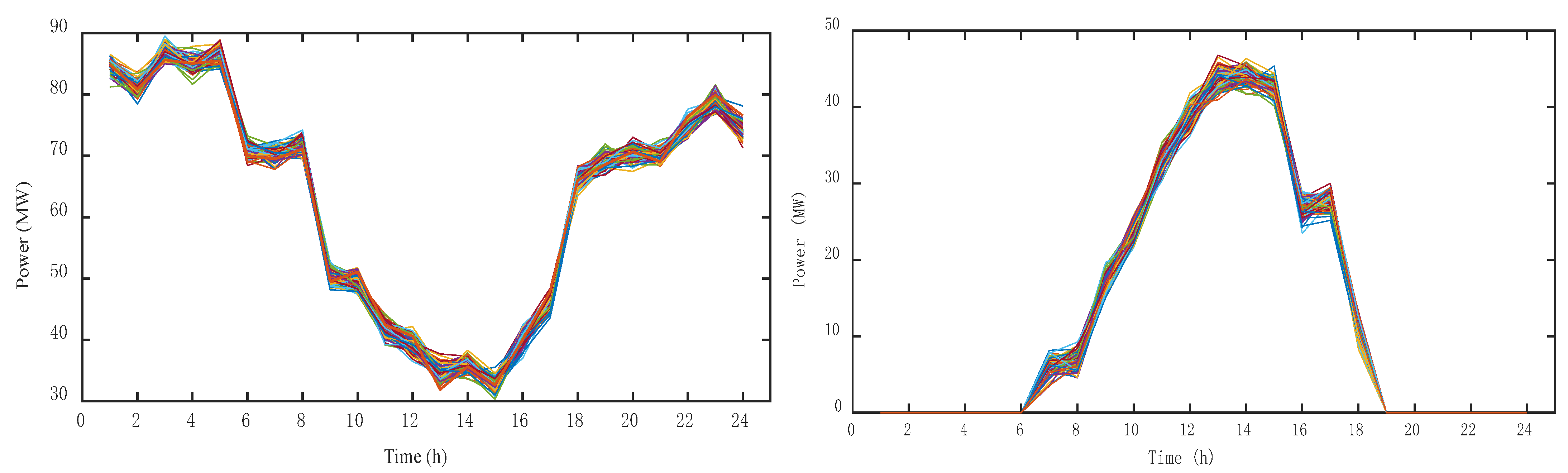
The curve of the cumulative probability distribution of the random variables X 1 , X 2 , X 3 , X 4 is used to generate a plurality of improved forecasts of the outputs of wind and photovoltaic power through Latin hypercube sampling [22].
(2)
These improved values are used to calculate the relative error in the predicted outputs of wind and photovoltaic power according to Equation (7) [23].
(3)
The error along with the formula f q , t = f t + e q , t = f t ( 1 + r e q , t ) is used to generate the predicted outputs of wind and photovoltaic power to form an initial scenario set.
(4)
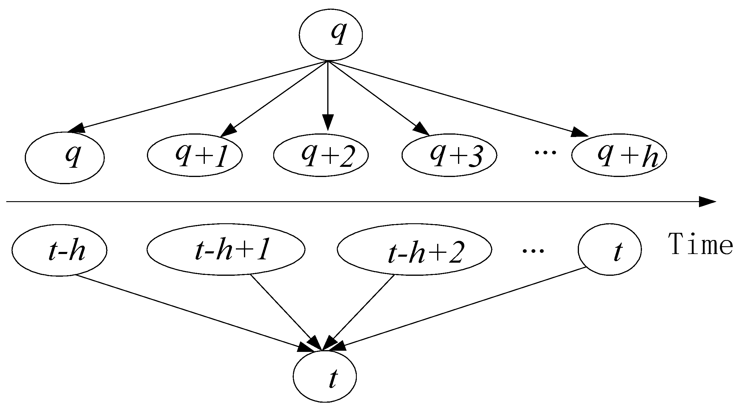
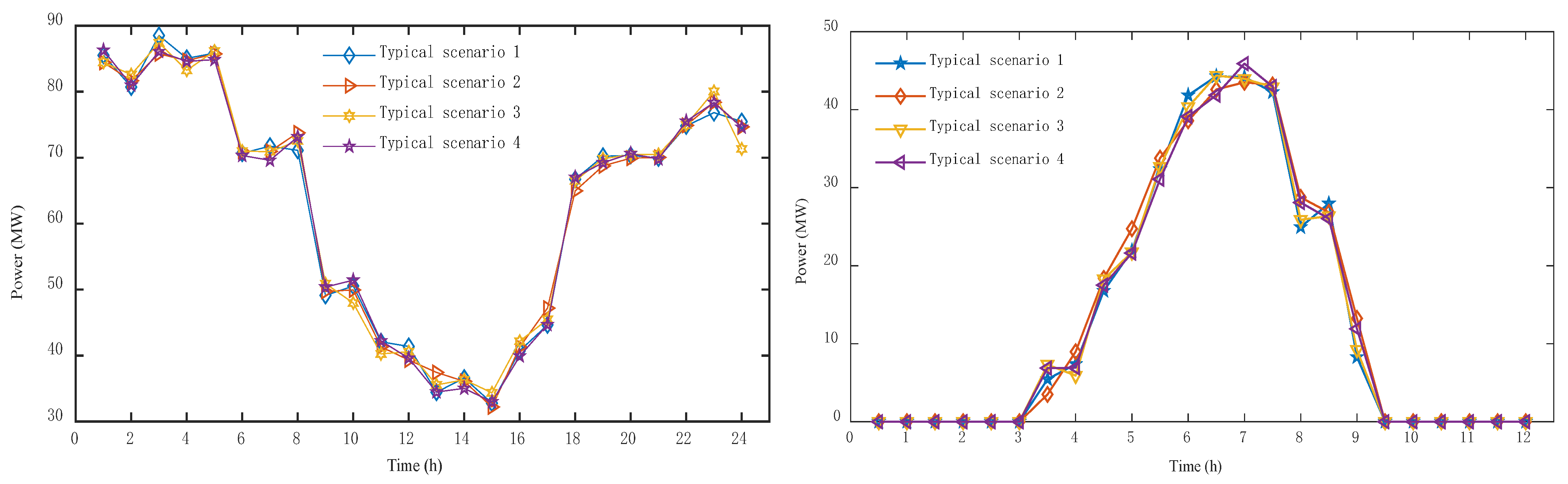
A typical scenario set of the outputs of wind and photovoltaic power is generated by the two-stage scenario reduction method [24].
(5)
The Cartesian product is used to varyingly combine the typical scenarios obtained above [7].
(6)
The Spearman correlation coefficient is used to determine the complementarity of wind and solar power in the combinations of scenarios, and the scenario with the optimal complementarity is selected.

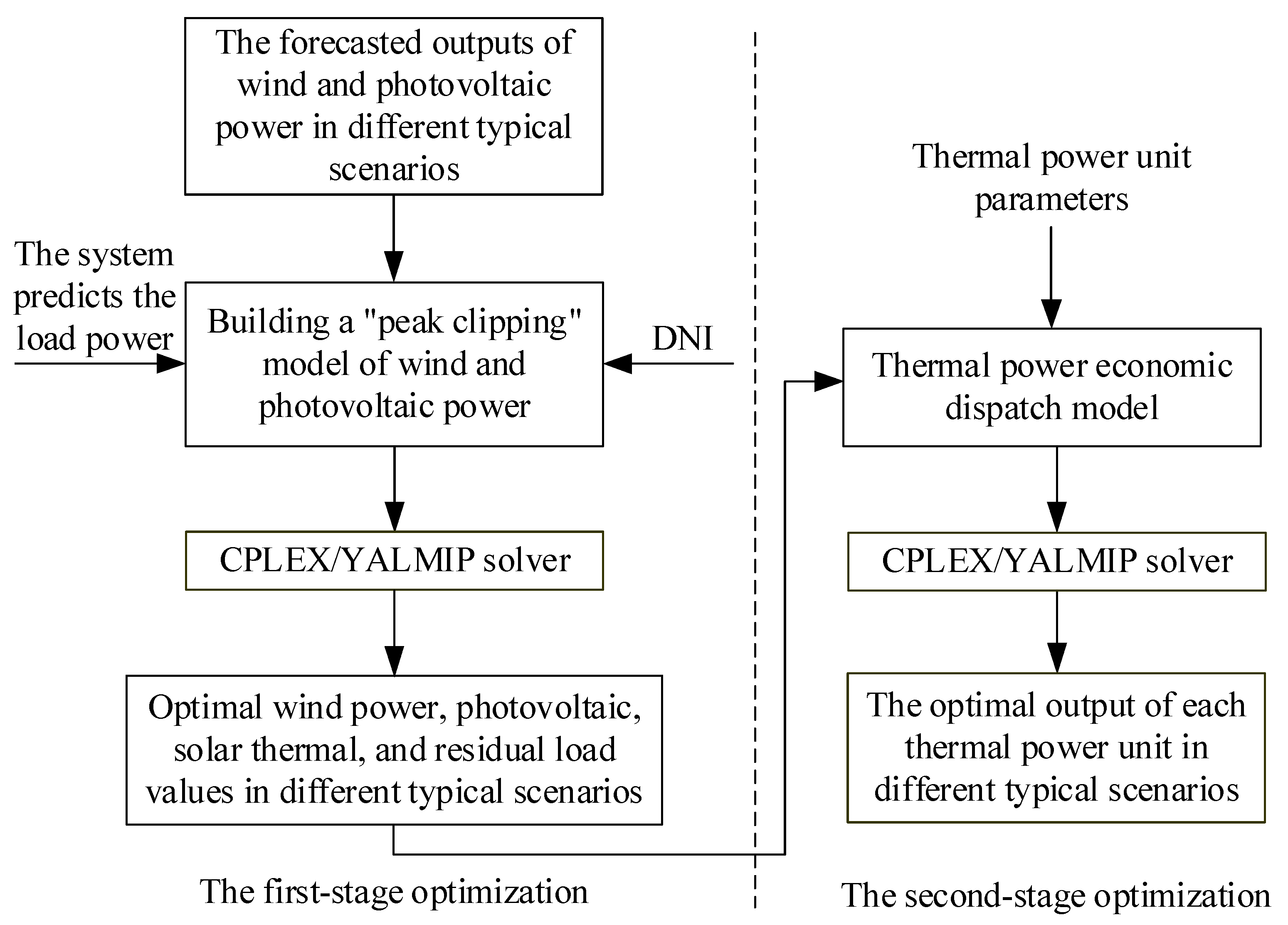
3. Two-Stage Optimal Model of Dispatch for a Combination of Wind Power, Photovoltaic Power, CSP, and Thermal Power Generation under Multiple Scenarios

The two-stage optimal scheduling model of wind power, photovoltaic power, CSP, and thermal power generation is shown as Figure 2.

3.1. First Stage of Optimization Model

Under a typical combination of scenarios of the forecasted outputs of wind and photovoltaic power, a “peak clipping” model of wind power, photovoltaic power, and CSP is established in the first stage of optimization. Its objectives are to maximize the daily power generation and minimize the difference between the peak and valley of the residual load. The model is solved by a solver to provide the residual loads in each period under different scenarios for the second stage of optimization. The objective function is as follows:
Objective function 1: Maximizing daily power generation:
max f 1 s = t = 1 T ( P w , t s + P p v , t s + P c s p , t s ) Δ t
Objective function 2: Minimizing the peak-to-valley difference of the residual load:
min f 2 s = max t T P l , t s min t T P l , t s P l , t s = P L , t P w , t s + P p v , t s + P c s p , t s )
In Equation (9), f 1 s , f 2 s respectively represent the daily power generation and the difference between the peak and valley of the residual load of the system for the combined generation of wind power, photovoltaic power, and CSP in different combinations of typical scenarios s ( s = 1 , 2 , 3 , 4 ) , T is the dispatch period, here set to 24, Δ t is the interval, set to one, P l , t s is the remaining load value in scenario s , and P w , t s , P p v , t s , P c s p , t s respectively represent the optimal outputs of wind power, photovoltaic power, and CSP at time t under scenario s .
The constraints are as follows:
(1)
Constraint on wind power output:
0 P w , t s P s , w , t
(2)
Constraint on photovoltaic power output:
0 P p v , t s P s , p v , t
In the above, P s , w , t , P s , p v , t are the predicted outputs of wind and photovoltaic power under scenarios s at time t , respectively.
(3)
Constraint on instantaneous thermal power balance of CSP station:
P t S F , s o l a r P t C S P , c u r t = ( P t T E S , c h a / η T E S , c h a P t T E S , d i s η T E S , d i s ) + P t P B , i n
In the above, P t S F , s o l a r is the thermal power collected by the heat collector, P t C S P , c u r t is the power needed for light curtailment, P t T E S , c h a , P t T E S , d i s are, respectively, the heat storage and heat release of the heat storage system, η T E S , c h a , η T E S , d i s are, respectively, the efficiencies of heat storage and heat release of the thermal storage system, and P t P B , i n is the thermal power entering the power generation system.
(4)
The equation of the heat energy balance of the heat collection system is:
P t S F , s o l a r = η S F S S F R t P t C S P , S H = P t S F , s o l a r P t C S P , c u r t
where η S F is the efficiency of photothermic, S S F is the area of the mirror field, and R t is the hourly direct solar radiation index (DNI).
(5)
The constraint on the functional relationship between the input thermal power and the output electric power of the power generation system is as follows:
P t P B , i n f ( P C S P , t ) = P C S P , t / η P B + U t P B E P B , S U
In the formula, P t C S P is the output of the electric power of the power generation system, η P B is its efficiency of power generation, U t P B is the state of the CSP station, and E P B , S U is the startup energy required for the CSP station to start generating electricity.
(6)
Constraint on the heat energy balance of the heat storage system:
E t T E S = ( 1 γ T E S ) E t 1 T E S + ( P t T E S , c h a P t T E S , d i s ) Δ t
In the formula, E t T E S is the heat storage capacity of the heat storage system at time t, E t 1 T E S is the heat storage capacity of the heat storage system at time t − 1, and γ T E S is the coefficient of heat dissipation.
(7)
Another constraint on the heat storage capacity of the heat storage system:
E min T E S E t T E S E max T E S
In the formula, E max T E S , E min T E S are the maximum and minimum heat storage capacities of the heat storage system, respectively.
(8)
The following are the constraints on the power storage and release of heat in the thermal storage system of the CSP station, where the storage and release of heat cannot be performed at the same time, and the state of heat release is restricted only when the unit is started:
0 P t T E S , c h a I t T E S , c h a P max T E S , c h a 0 P t T E S , d i s I t T E S , d i s P max T E S , d i s I t T E S , c h a + I t T E S , d i s 1 , x t P B I t T E S , d i s
where P max T E S , c h a , P max T E S , d i s are the maximum heat storage and heat release power of the heat storage system, respectively. I t T E S , c h a , I t T E S , d i s are the binary variables of heat storage and heat release, respectively, “1” means that the system is storing heat and “0” means that it is releasing heat, and x t P B is the variable of the working state of the CSP station, where “1” means that it has been turned on.
(9)
Constraints on the output of the CSP station:
x t P B P min P B P c s p , t s x t P B P max P B
where P max P B , P min P B are the maximum and minimum outputs of the CSP, respectively.
(10)
Constraints on the minimum start and stop times of the CSP unit:
( x t P B x t 1 P B ) T min o n , c s p + τ = t T min o n , c s p t 1 x τ P B 0 ( x t 1 P B x t P B ) T min o f f , c s p + τ = t T min o f f , c s p t 1 ( 1 x τ P B ) 0
where T min o n , c s p , T min o f f , c s p are the minimum start and stop times of the CSP unit, respectively.
(11)
Constraints on the relationship between the variables of the state of operation of the CSP station, and those of the start and stop times are as follows:
x t P B x t 1 P B u t P B x t 1 P B x t P B v t P B
where u t P B , v t P B are the start and stop variables of the CSP unit, respectively, and “1” indicates that the unit is in the start or stop state.
(12)
Constraints on the ramp rate of the CSP unit:
P c s p , t s P c s p , t 1 s + x t 1 P B ( P min P B P R U P B ) + x t P B ( P max P B P min P B ) P max P B P c s p , t 1 s P c s p , t s + x t P B ( P min P B P R D P B ) + x t 1 P B ( P max P B P min P B ) P max P B
where P R U P B , P R D P B are the upward and downward ramp rates of the solar thermal unit, respectively.

3.2. Second Stage of the Optimization Model

The conventional thermal power unit was used to bear the remaining load in the second stage of optimization. The objective was to minimize the operating cost of the thermal power unit, and an economical dispatch model was established for this purpose. The model was also solved by a solver, and the dispatched output of each thermal power unit in different typical combinations of scenarios was obtained. The objective function is as follows:
Objective function 3: Minimizing the operating cost of thermal power unit:
min f 3 s = t = 1 T i = 1 N G [ u i , t s F i ( P G , i , t s ) + u i , t s ( 1 u i , t 1 s ) S i ] F i ( P G , i , t s ) = a i ) P G , i , t s ) 2 + b i P G , i , t s + c i
where f 3 s represents the operating costs of the thermal power unit in different typical scenarios s , P G , i , t s is the dispatched output of the first thermal power unit in s , and u i , t s is the state of the thermal power unit in s , where “1” means start-up and “0” means shutdown. S i is the cost of starting-up the first thermal power unit, a i , b i , c i are the coefficients of its fuel cost, and N G is the number of thermal power units.
The constraints are as follows:
(13)
Constraints on the power balance of the system:
i = 1 N G P G , i , t s = P l , t s
(14)
Constraints on the output of the thermal power units:
u i , t s P G , i min P G , i , t s u i , t s P G , i max
where P G , i min , P G , i max are the minimum and maximum outputs of each thermal power unit, respectively.
(15)
Constraints on climbing on thermal power units:
u i , t s R i d P G , i , t s P G , i , t 1 s u i , t s R i u
where R i d , R i u are the downward and upward climbing rates of each thermal power unit, respectively.
(16)
Constraints on the minimum starting and stopping times of thermal power units:
( T i , o n t 1 T i , o n min ) ( U i , t 1 U i , t ) 0 ( T i , o f f t 1 T i , o f f min ) ( U i , t U i , t 1 ) 0
where T i , o n t is the continuous start-up time of the first thermal power unit, T i , o f f t is its continuous shutdown time, T i , o n min is its minimum start-up time, and T i , o f f min is the minimum shutdown time of the first thermal power unit.

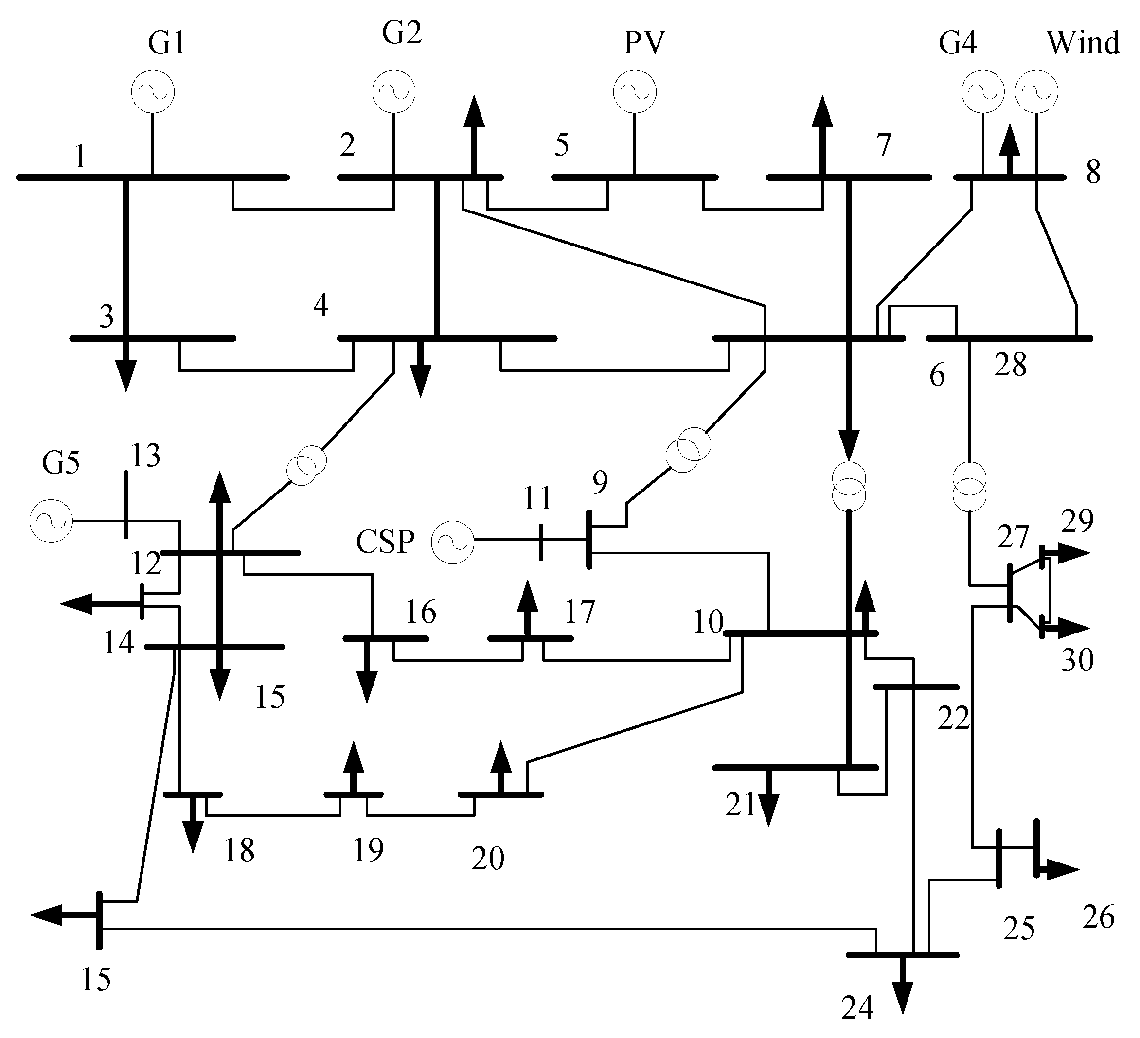
4. Example for Analysis

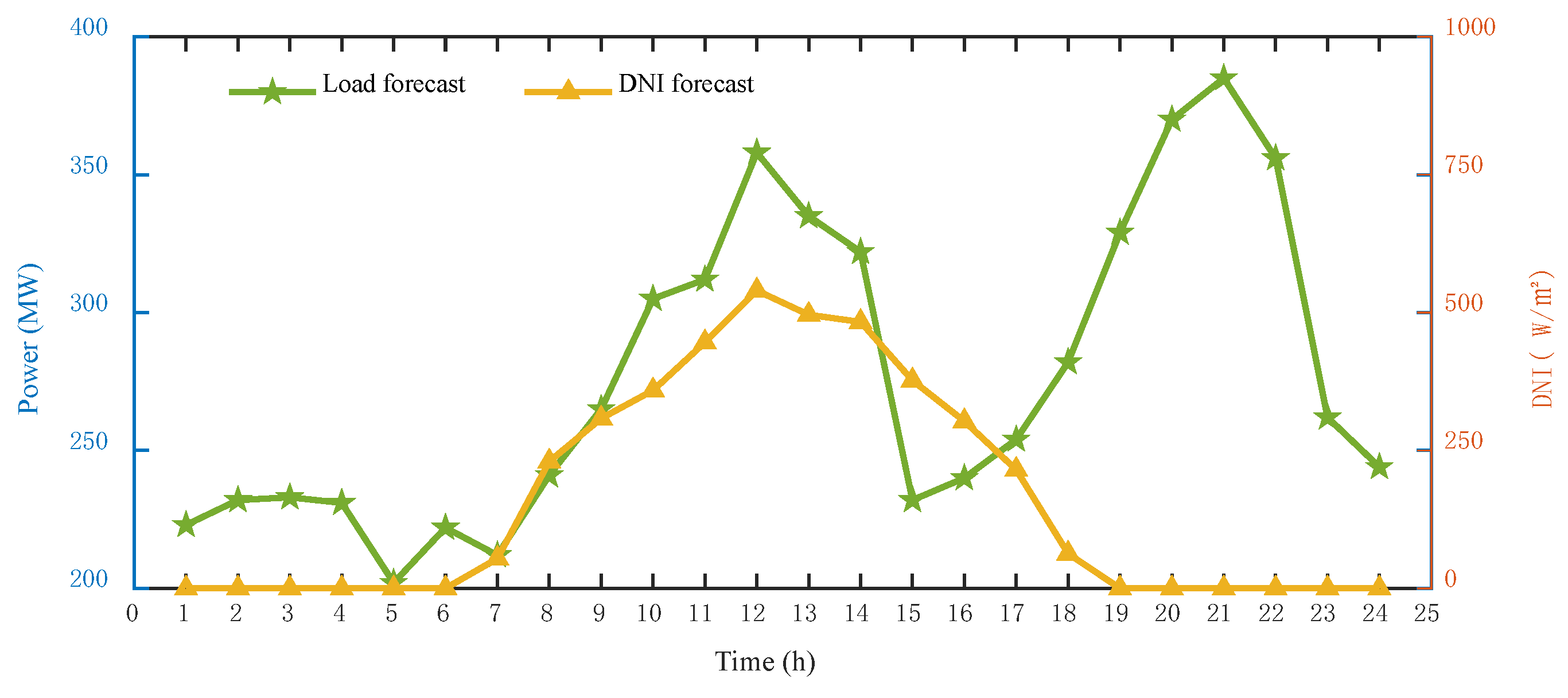
4.1. Basic Data and Parameters

We used the IEEE 30 bus system as an example to analyze the proposed system. The system considered here contained four conventional thermal power units, a wind farm with an installed capacity of 90 MW, a photovoltaic power station with an installed capacity of 50 MW, and a CSP station with an installed power of 50 MW. The wiring diagram of the system is shown in Figure 3. The parameters of the four thermal power units are shown in Table 1 and the operating parameters of the CSP station are shown in Table 2. Because the forecasted error in load was smaller than those in the wind and photovoltaic power, the uncertainty of load was not considered. The typical daily forecasted load and DNI are shown in Figure 4.

4.2. Analysis of Results of Example

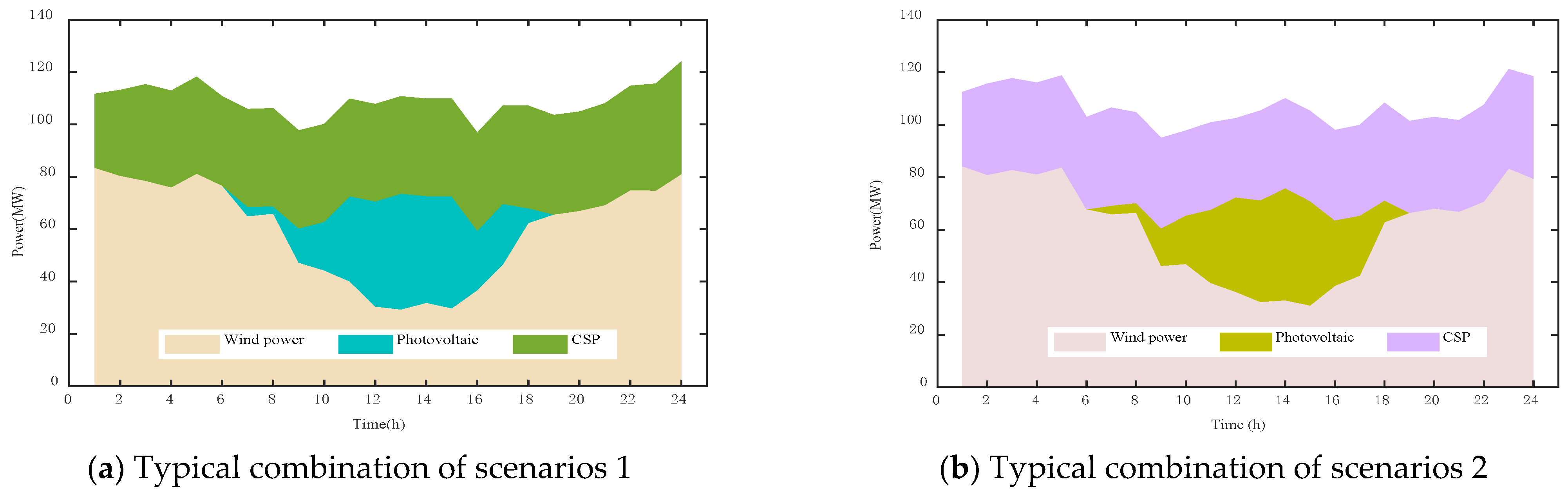
4.2.1. Generation of Typical Combined Scenarios

A wind farm and a photovoltaic power station in the Dunhuang area of Gansu Province were selected as research objects. We used data on the predicted and actual outputs of wind and photovoltaic power on a typical day that were collected every hour. Through a statistical analysis of predictions of the outputs of wind and photovoltaic power, 1920 improved values were randomly generated by using Latin hypercube sampling. The error in these predictions was obtained by combining them with Equation (7). This led to 100 scenarios of predictions of the outputs of wind and photovoltaic power. We then used the two-stage scenario reduction method to obtain four groups of scenarios, as shown in Figure 5.
The Cartesian product was used to combine typical scenarios of the outputs of forecasts of wind and photovoltaic power to obtain 16 combinations of scenarios [7]. The Spearman correlation coefficient was used to analyze the complementarity among the four typical scenarios of each group. The correlation coefficient of the outputs of wind and photovoltaic power under different scenarios were shown in Table 3.
From Table 3, we can see the complementarity of wind and photovoltaic power is different in different combined scenarios. Four combined scenarios with the strongest complementarity were then selected. They respectively corresponded to the typical combined scenarios 1, 2, 3, and 4.

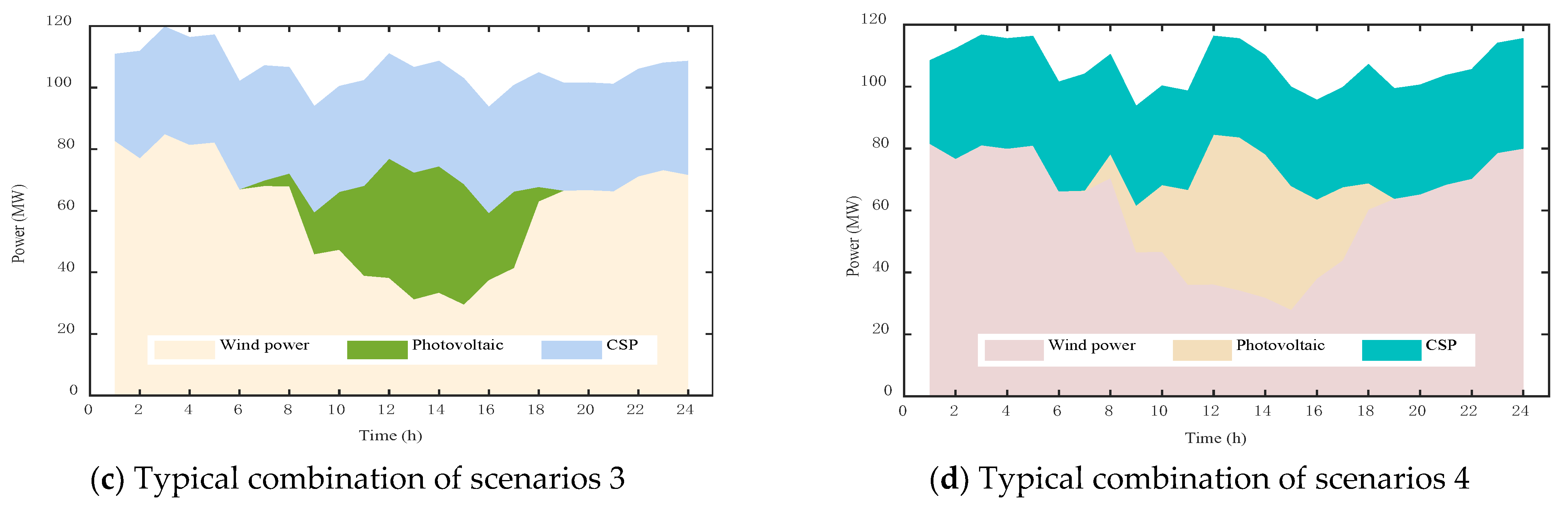
4.2.2. Analysis of Optimal Outputs of Wind Power, Photovoltaic Power, and CSP under Different Typical Combinations of Scenarios in the First Stage

Based on the different outputs of wind energy and photovoltaic power generation prediction under these typical scenario combinations, Gurobi solver is used to solve the joint “peak shearing” model of wind power, photovoltaic, and CSP under different typical scenario combinations. The optimal outputs of wind power, photovoltaic power, and CSP under different typical combinations of scenarios are shown in Figure 6.
Figure 6 shows the optimal outputs of the dispatch of wind power, photovoltaic power, and CSP in each period under each typical combination of scenarios. It shows that the photovoltaic power station did not generate electricity when the light intensity was insufficiently strong or when there was no light. Owing to the high wind speed at night, the output of the wind farm was higher than that in daytime. The CSP station had a heat storage system that allowed it to transfer power generation to the periods of sunrise and sunset. Therefore, at night, when the output of wind power generation fluctuated significantly, the CSP station could generate electricity through the heat storage system to alleviate this situation. In the daytime, especially when the light intensity was sufficiently strong—for example, from 11:00 to 16:00—the output of wind power was small while those of the photovoltaic power station and CSP station were large such that they could compensate for the shortage of the generated wind power.

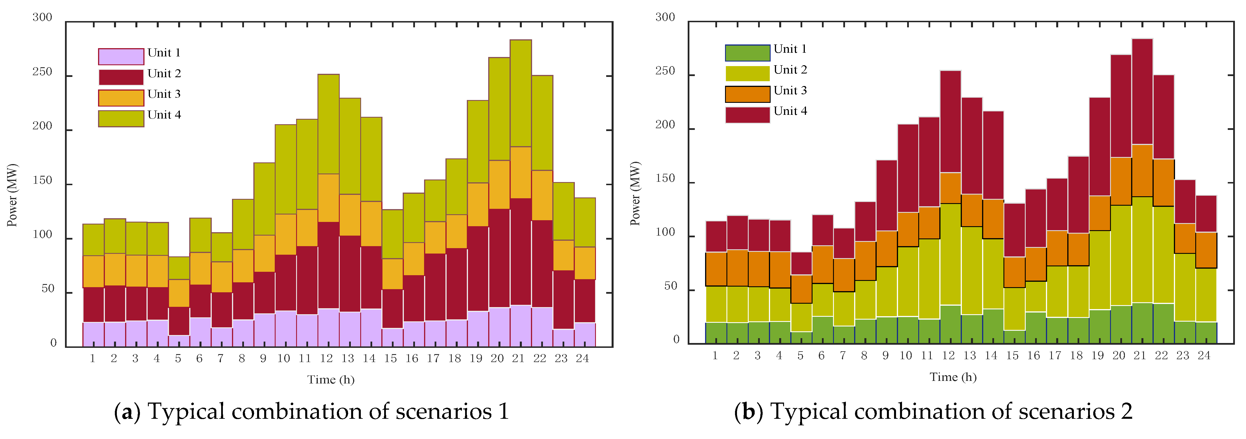
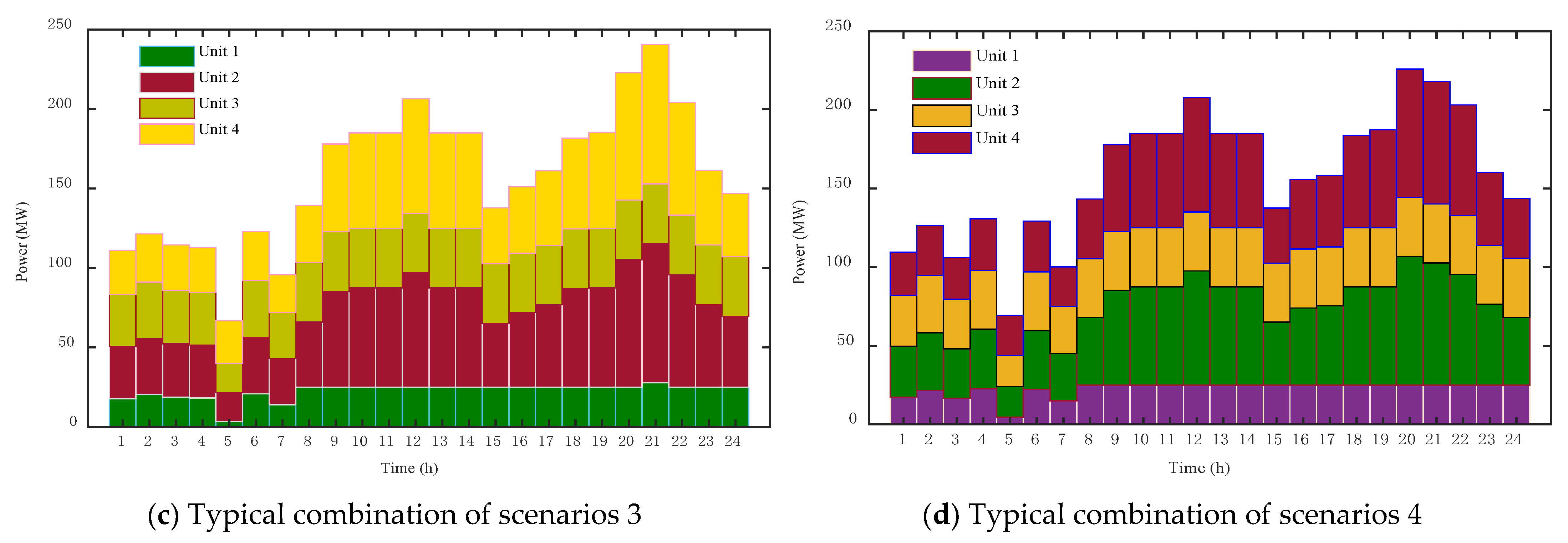
4.2.3. Analysis of the Optimal Outputs under Different Typical Combinations of Scenarios in the Second Stage of Optimization

Calculations from the first stage of scheduling of the model were used to obtain the values of the remaining load in each interval under different typical combinations of scenarios. The residual load values of each time period under different typical scenario combinations are introduced into the second stage, and the economic dispatch model of thermal power in the second stage is solved by Gurobi to obtain the optimal output of each thermal power unit in each time period under each typical scenario combination, as shown in Figure 7.
Figure 7 shows that under different typical combinations of scenarios, the output of each thermal power unit exhibited the same trend. The higher the cost of thermal power unit 1 was, the smaller was the output of the unit, while the lower the cost of thermal power unit 4 was, the larger was the output. During the period of peak load from 10:00 to 14:00, the thermal power unit needed to adjust the output to compensate for the shortage of wind power because this was small while the photovoltaic power and CSP were large. During the period of a valley in the load from 0:00 to 6:00, the output wind power was large and the output of photovoltaic power was zero. At this time, the latter was compensated for by CSP generation while the output due to thermal power was small.

4.2.4. Analysis of Influence of Complementarity of Wind and Photovoltaic Power on Results of Dispatch

Wind and solar energy have naturally complementary characteristics. Due to the changes in its speed, the energy generated from wind power is the largest at night and the smallest in the daytime. Photovoltaic power can be used to generate electricity only in the daytime. Moreover, the greater the intensity of solar radiation, the greater the output of photovoltaic power. The optimal combination of their forecasted outputs was selected and used in the scheduling model. The impact of the complementarity of the outputs of wind and solar power on the results of scheduling was then analyzed through optimization calculations. Table 4 shows a comparison of the parameters of optimization under different typical combinations of scenarios.
Table 4 shows that among four typical combinations of scenarios, the peak–valley difference in the residual load was reduced by 5.497 MW in comparison with the typical combination of scenario 4, with weaker complementarity in other typical combination of scenarios, because the complementarity of the outputs of wind and photovoltaic power in the typical combination in scenarios 1 was stronger than those in the other scenarios. The volume of wind curtailment and the quantity of its curtailment in the typical combination of scenarios 1 were 78.284 MW and 36.877 MW, respectively, where the volume and quantity of wind curtailment were reduced by 18.56% and 8.25%, respectively. By complementing the outputs of wind and photovoltaic powers in different periods, the fluctuations in them were reduced such that the curtailing of the volume of wind was reduced. The cost of operation of thermal power in the typical combination of scenarios 1 was reduced by 43.96% compared with that in the typical combination of scenarios 4 because the outputs of wind and photovoltaic power of the former had the highest complementarity. This led in turn to improved regulation of the photo-thermal power station and increased the on-grid electricity due to wind and photovoltaic powers. When the wind and photovoltaic powers were used to satisfy the peak load, only thermal power was used to meet the base load to reduce the power generation of the thermal power units. Their costs of operation and power generation were thus further reduced.

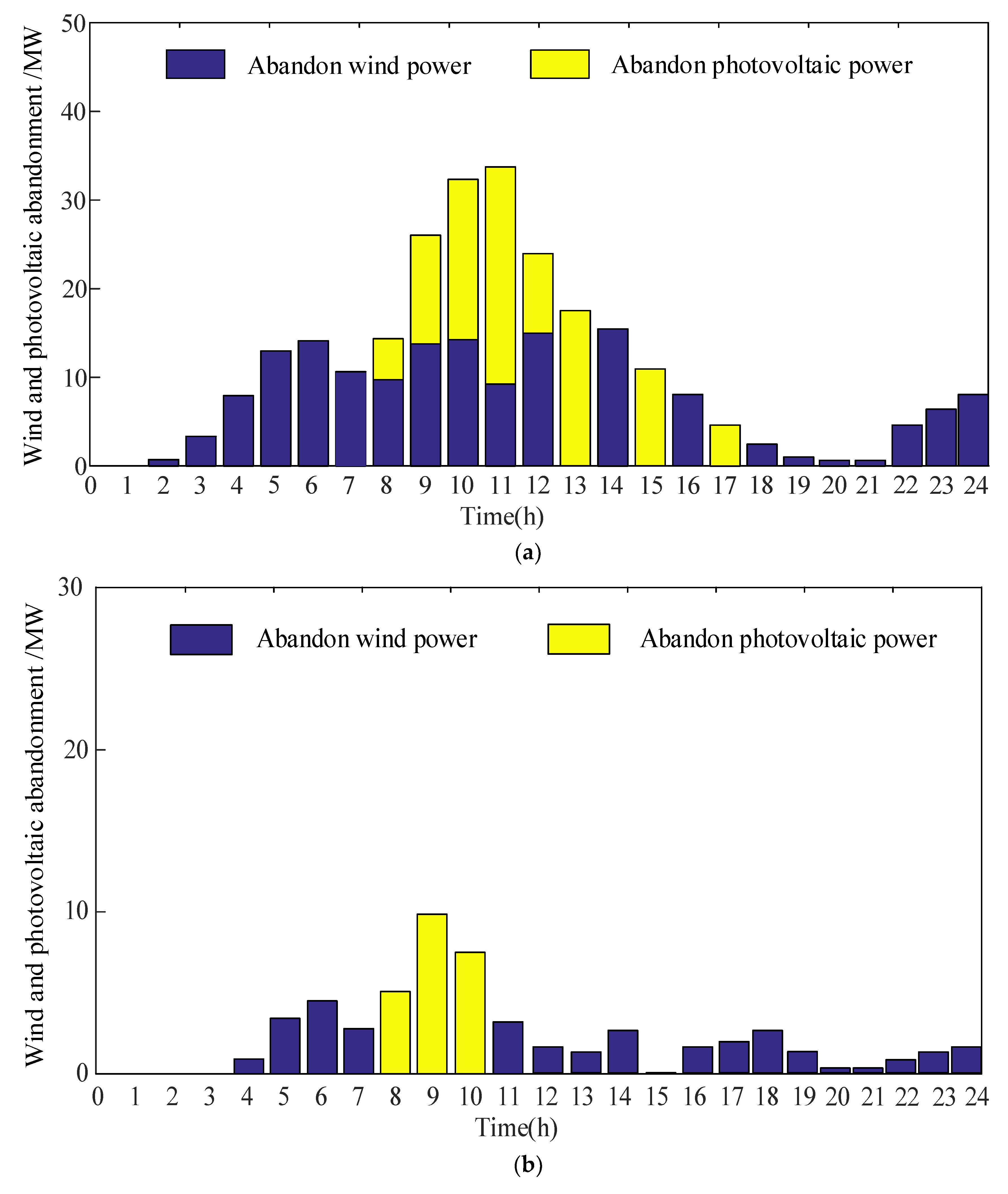
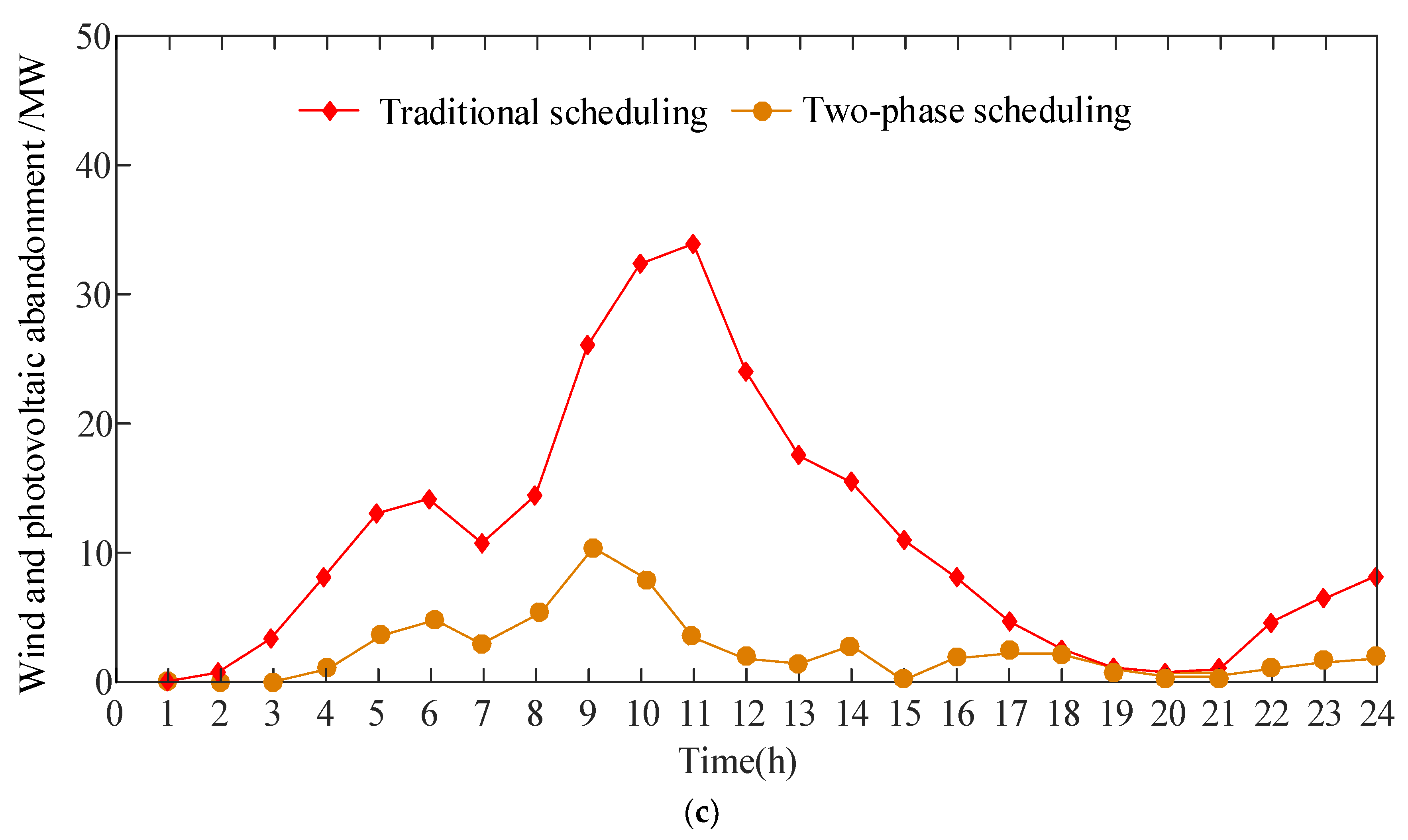
4.2.5. Comparative Analysis of Different Scheduling Modes

To verify the effectiveness of the scheduling strategy proposed in this paper, we conducted a comparative analysis of different scheduling modes:
Dispatching mode 1: This involved an integrated, multi-source method of grid connection that dispatched wind power, photovoltaic power, CSP, and thermal power. Only wind, photovoltaic, and thermal power were assumed to participate in grid dispatching. Therefore, the set of dispatching modes 1 did not consider the uncertainty of the outputs of wind and solar power and assumed the natural output of the solar thermal power station.
Dispatching mode 2: This dispatching strategy optimized the output of each power source in stages, but there was no grid-connected CSP station. This was regulated by a conventional thermal power station to alleviate the uncertainty in the outputs of wind and photovoltaic power. This mode also did not consider the uncertainty in these outputs when establishing the model.
Dispatching mode 3: Proposed model of scheduling
The optimized cost of operation of thermal power, the penalty cost of curtailment of wind and solar power, the rates of such curtailments, and the cost of dispatching under each dispatching mode were compared and analyzed. Table 5 shows a comparison of the parameters of optimization under different scheduling modes.
The comparison in Table 5 shows that because dispatching modes 1 and 2 both considered the same scenario, the deterministic dispatching model was established for them, while dispatching mode 3 was a stochastic dispatching model established in different scenarios. Although the CSP of dispatching mode 1 did not participate in power grid dispatching, it was a natural output. However, compared with the second dispatch, there was no CSP output, and only thermal power units were used to smooth the uncertainty of the outputs of wind and solar power. This increased the difficulty of operation of the thermal power unit. These units need to start and stop frequently to adjust such outputs. The increase in the output of the thermal power unit led to an increase in the cost of coal consumed, which in turn increased the operational cost of thermal power and the cost of dispatch of the system. Both dispatching modes 1 and 3 used photo-thermal grid-connected power generation, but compared with dispatching mode 1, which considered only the natural output of photo-thermal energy, dispatching mode 3 considered the uncertainty in the predicted outputs of wind and solar power in addition to adopting the complementary regulation of thermal and photo-thermal powers. Compared with dispatching mode 1, the thermal power operation cost, wind and light abandonment penalty cost, and dispatching cost of dispatching mode 3 are reduced by 52.685%, 4.032%, and 50.156%, respectively. In terms of the total wind and light abandonment rate, the dispatching mode 3 is 2.289% and 8.167% lower than that of the dispatching mode 1 and 2, respectively.
In order to verify the effectiveness of the proposed method in this paper, the wind and photovoltaic curtailment power in the traditional scheduling and the two-phase scheduling are shown as Figure 8.
Figure 8 is the wind and photovoltaic abandonment. (a) is the amount of wind and light curtailment under the traditional scheduling. The wind curtailment is mainly concentrated at 03:00 to 12:00, and the light curtailment is concentrated in 08:00 to 13:00 and 15:00. Under this traditional model, the amount of wind and light curtailment is more; (b) is for the two-stage scheduling, the amount of wind and light abandonment is mainly concentrated in 04:00 to 07:00 and 11:00, and the curtailment of light is concentrated in 08:00 to 10:00, the amount of curtailment of wind and light under this two-stage model is significantly reduced, and there is no curtailment of wind and light at other times; (c) is for the comparison of the amount of wind and light curtailment under the traditional scheduling and the two-stage scheduling. It can be seen that the model proposed in this paper significantly improves the problem of excessive wind and light curtailment under traditional scheduling, provides a basis for joint optimization scheduling, and has certain practical significance.

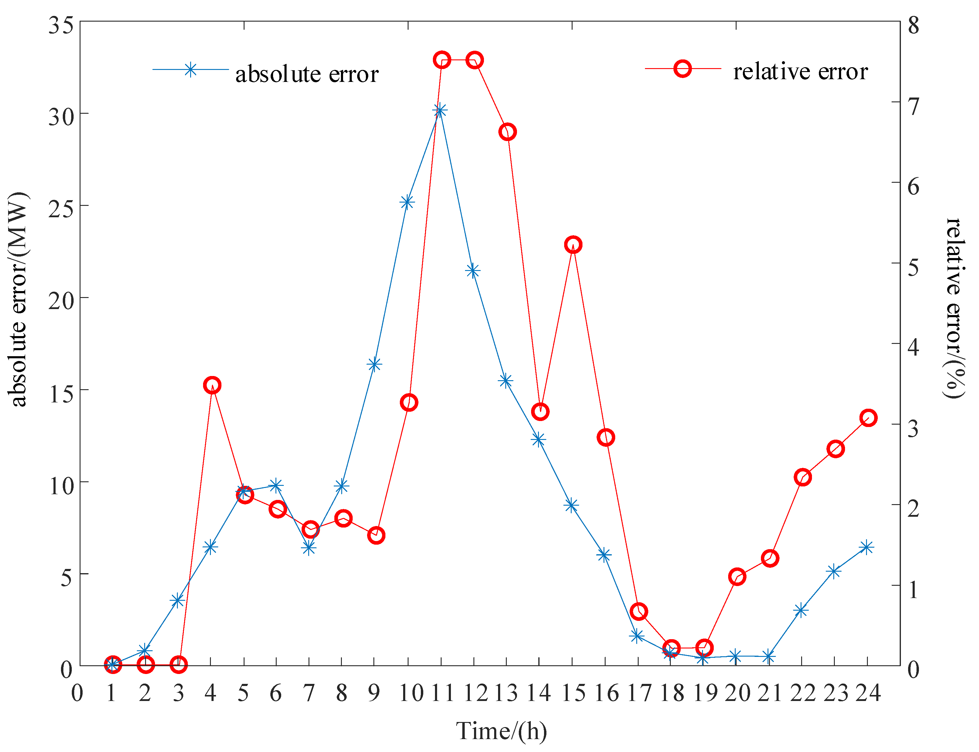
4.2.6. Comparison between Relative Error and Absolute Error

Figure 9 shows the comparison of relative error and absolute error, and the two errors reached the maximum at 11:00, 30.12 MW and 7.51%, respectively. The relative error is mainly below 8%, which further illustrates the superiority of the proposed model.

5. Conclusions

In this paper, under the premise of considering the uncertainty of wind and solar forecast output, the optimal scheduling strategy of the multi-energy combined system that CSP plants participate in is proposed. Conclusions are as follows:
(1)
Aiming at the uncertainty problem of wind and solar prediction output, on the basis of the traditional martingale model, this paper proposes an improved martingale model to analyze the uncertainty of the wind and solar prediction output by replacing the absolute error value in the traditional martingale model with the relative error of prediction.
(2)
Through Latin hypercube sampling and two-stage scene reduction technology, a typical wind and solar prediction output scenario is generated. Then, the Cartesian product idea is used to combine the typical scene of the generated wind and solar prediction output. The Spearman correlation coefficient is used as an indicator to quantitatively analyze the complementarity of the wind and solar prediction output in the combination scenario. The combination of the wind and solar prediction output with the best complementarity is selected to form different typical combination scenarios.
(3)
A two-stage coordinated dispatch model of wind-solar-thermal combined power generation system under different combination scenarios is established. Different scheduling modes are set for comparison and analysis.

Author Contributions

Data curation, M.X.; Formal analysis, T.W. and X.Z.; Resources, Y.Z.; Software, Y.C. and Y.G. All authors have read and agreed to the published version of the manuscript.

Funding

This work is supported by Gansu Province Electric Power Company cooperation project (No. SGTYHT/21-WT-256).

Data Availability Statement

The data that support the findings of this study are available from the corresponding author upon reasonable request.

Conflicts of Interest

The authors declare no conflict of interest.

References

  1. Li, C.H.; Jiang, M.; Yao, D.G.; Ge, H.C.; Zhang, Z.A.; Tang, L. Rolling dispatching method of two-stage reactive power in high proportion renewable energy power system. China South. Power Grid Technol. 2022, 16, 94–103. [Google Scholar]
  2. Du, E.S.; Zhang, N.; Kang, C.Q.; Shen, M. Reviews and Prospects of the Operation and Planning Optimization for Grid Integrated Concentrating Solar Power. Proc. CSEE 2019, 36, 5765–5775. [Google Scholar]
  3. Liu, Y. Research on Optimal Dispatch of Multi Source Power Generation System with Electric Heater and Concentrating Solar Power Plant. Master’s Thesis, East China Jiaotong University, Nanchang, China, 2021. [Google Scholar]
  4. Huang, K.L. Robust Optimization Design for Fatigue Life of a Car Body Based on Weibull Distribution. Master’s Thesis, Jilin University, Jilin, China, 2021. [Google Scholar]
  5. Li, P.; Guan, X.H.; Wu, J. Wind Power Scenario Generation for Multiple Wind Farms Based on Atmospheric Dynamic Model. Proc. CSEE 2016, 35, 4581–4590. [Google Scholar]
  6. Tian, Y.Y. Hydropower, Thermal Power, Wind Power and Photovoltaic Joint Dispatch Considering Uncertainty. Master’s Thesis, Xi’an University of Technology, Xi’an, China, 2020. [Google Scholar]
  7. Zhang, J.T.; Cheng, C.T.; Shen, J.J.; Li, G.; Li, X.F.; Zhao, Z.Y. Short-term Joint Optimal Operation Method for High Proportion Renewable Energy Grid Considering Wind-solar Uncertainty. Proc. CSEE 2020, 40, 5921–5932. [Google Scholar]
  8. Wang, Q.; Dong, W.L.; Yang, L. A Wind Power/Photovoltaic Typical Scenario Set Generation Algorithm Based on Wasserstein Distance Metric and Revised K-medoids Cluster. Proc. CSEE 2019, 35, 2654–2661. [Google Scholar]
  9. Zhang, Z.S.; Sun, Y.Z.; Gao, D.W.; Lin, J.; Cheng, L. A Versatile Probability Distribution Model for Wind Power Forecast Errors and Its Application in Economic Dispatch. IEEE Trans. Power Syst. 2021, 28, 3114–3125. [Google Scholar] [CrossRef]
  10. Jiang, Y.W.; Chen, C.; Wen, B.Y. Particle Swarm Research of Stochastic Simulation for Unit Commitment in Wind Farms Integrated Power System. Trans. China Electrotech. Soc. 2019, 24, 129–137. [Google Scholar]
  11. Zhao, S.Q.; Wang, H.; Zhang, H. Wind Farm and Photovoltaic Power Station Output Time Series Model Considering Correlation. Smart Power 2020, 48, 52–58+87. [Google Scholar]
  12. Luo, X.Y. Reliability Evaluation of Distribution Network Considering the Relevance of Wind Far. Master’s Thesis, Taiyuan University of Science and Technology, Taiyuan, China, 2021. [Google Scholar]
  13. Li, J.H.; Wen, J.Y.; Cheng, S.J.; Wei, H. A Scene Generation Method Considering Copula Correlation Relationship of Multi-wind Farms Power. Proc. CSEE 2019, 33, 30–36+21. [Google Scholar]
  14. Xu, J.; Hong, M.; Sun, Y.Z.; Zhou, G.H. Dynamic scenario generation based on empirical Copula function for outputs of multiple wind farms and its application in unit commitment. Electr. Power Autom. Equip. 2019, 37, 81–89. [Google Scholar]
  15. Cai, J.; Wang, Y.T.; Xu, X.Q. Joint optimization model of power grid unit combination and technical transformation plan considering transmission and distribution coordination. Electr. Power Autom. Equip. 2022, 1–25. [Google Scholar] [CrossRef]
  16. Pan, Y.Y. Optimal Scheduling Research of Power System considering Concentrating Solar Power Plant Participation. Master’s Thesis, Lanzhou Jiaotong University, Lanzhou, China, 2020. [Google Scholar]
  17. Zhao, T.; Cai, X.; Yang, D. Effect of streamflow forecast uncertainty on real-time reservoir operation. Adv. Water Resour. 2011, 34, 495–504. [Google Scholar] [CrossRef]
  18. Zhao, T.; Zhao, J.; Yang, D.; Hao, W. Generalized martingale model of the uncertainty evolution of streamflow forecasts. Adv. Water Resour. 2013, 57, 41–51. [Google Scholar] [CrossRef]
  19. Chen, L.; Lu, W.W.; Zhou, J.Z.; Guo, S.L.; Guo, H.J. Effect of streamflow forecast uncertainty on reservoir operation. J. Hydraul. Eng. 2016, 47, 77–84. [Google Scholar]
  20. Xu, B.; Zhu, F.; Zhong, P.A.; Chen, J.; Deng, X. Identifying long-term effects of using hydropower to complement wind power uncertainty through stochastic programming. Appl. Energy 2019, 253, 113535. [Google Scholar] [CrossRef]
  21. Liu, W.; Zhu, F.; Zhao, T.; Wang, H.; Fthenakis, V. Optimal stochastic scheduling of hydropower-based compensation for combined wind and photovoltaic power outputs. Appl. Energy 2020, 276, 115501. [Google Scholar] [CrossRef]
  22. Li, L.; Xia, J.; Xu, C.; Singhde, V.P. Evaluation of the subjective factors of the GLUE method and comparison with the formal Bayesian method in uncertainty assessment of hydrological models. J. Hydrol. 2020, 390, 210–221. [Google Scholar] [CrossRef]
  23. Cheng, J.H. Research on Optimal Dispatching of Regional Power Grid Including Wind and Solar Energy Storage. Master’s Thesis, North China Electric Power University, Beijing, China, 2021. [Google Scholar]
  24. Yan, B.W.; Guo, S.L.; Chen, L. Estimation of reservoir flood control operation risks with considering inflow forecasting errors. Stoch. Environ. Res. Risk Assess. 2021, 28, 359–368. [Google Scholar] [CrossRef]
Figure 1. The evolution of the outputs of wind and photovoltaic power over time.
Energies 15 08215 g001
Figure 2. Two-stage optimal scheduling model of wind-photovoltaic-thermal-thermal power combined power generation system.
Energies 15 08215 g002
Figure 3. Wiring diagram of IEEE 30 bus system.
Energies 15 08215 g003
Figure 4. Typical forecasted daily load and DNI.
Energies 15 08215 g004
Figure 5. Scenario set of forecasted outputs of wind and photovoltaic power.
Energies 15 08215 g005aEnergies 15 08215 g005b
Figure 6. Optimal outputs of wind power, photovoltaic power, and CSP under four typical combinations of scenarios.
Energies 15 08215 g006aEnergies 15 08215 g006b
Figure 7. Optimal output of each thermal power unit under each typical combination of scenarios.
Energies 15 08215 g007aEnergies 15 08215 g007b
Figure 8. Wind and photovoltaic abandonment. (a) Wind and photovoltaic curtailment power under Traditional scheduling, (b) Wind and photovoltaic abandonment under Two-phase scheduling, (c) The comparison of Wind and photovoltaic abandonment in Traditional scheduling and Two-phase scheduling.
Energies 15 08215 g008aEnergies 15 08215 g008b
Figure 9. Comparison between relative error and absolute error.
Energies 15 08215 g009
Table 1. Parameters of the thermal power units.
UnitOutput Upper Limit/MWOutput Lower Limit/MWUnit Ramp Rate/MW·h−1Efficiency of Fuel Cost
ai/¥·MW−2bi/¥·MW−1ci/¥
14010300.30.2713.7
210025301.40.2614.5
35025406.10.286.35
410020400.80.2714.1
Table 2. Operating parameters of optimal thermal power station.
Operational Parameters of CSP StationValue
Rated output power of CSP station/MW50
Minimum output power of CSP station/MW10
Climbing rate of CSP station/MW/h40
Rate of heat release loss of TES/%0.57
Thermal power conversion efficiency of CSP station/%0.45
Maximum heat storage capacity/MWh1000
Initial value of heat storage capacity of TES/MWh400
Lower limit of TES/MWh100
Table 3. The correlation coefficient of the outputs of wind and photovoltaic power under different scenarios.
PV1PV2PV3PV4
WF1−0.9409−0.9427−0.9495−0.9353
WF2−0.9428−0.9431−0.9491−0.9354
WF3−0.9531−0.9502−0.9643−0.9441
WF4−0.9451−0.9475−0.9522−0.9416
Table 4. Comparison of optimization parameters in different typical scenarios.
Typical Combination of ScenariosResidual Load Peak–valley Difference/MWAbandoned Wind
Quantity/MW
Abandoned Photovoltaic
Quantity/MW
Thermal Power Operation
Cost/yuan
1132.96478.28436.877103,543.898
2136.02181.39338.383104,352.931
3138.00881.92438.919184,698.118
4138.46196.11940.194184,779.507
Table 5. Comparison of the optimization parameters under different scheduling modes.
ModeThermal Power Operation
Cost/yuan
Abandoned Wind and Light
Penalty Cost/yuan
Total Wind Curtailment and Light Abandonment Rate/%Scheduling
Cost/yuan
Mode 1218,840.18512,00019.971230,840.185
Mode 2238,231.04616,996.92425.849255,227.9703
Mode 3103,543.89811,516.14217.682115,060.040
Publisher’s Note: MDPI stays neutral with regard to jurisdictional claims in published maps and institutional affiliations.

