

Smart Gas Network with Linepack Managing to Increase Biomethane Injection at the Distribution Level


Abstract
1. Introduction
2. Materials and Methods
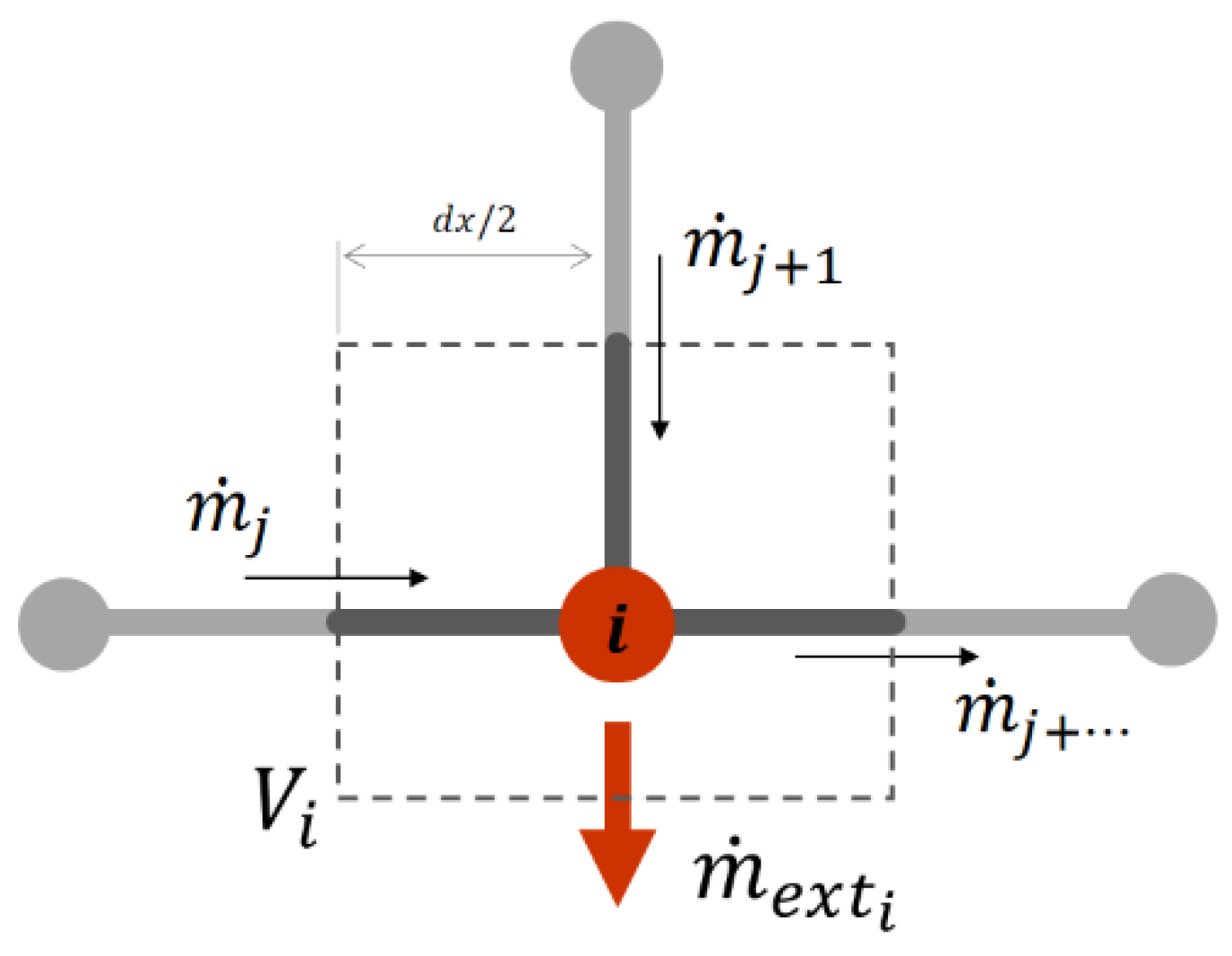
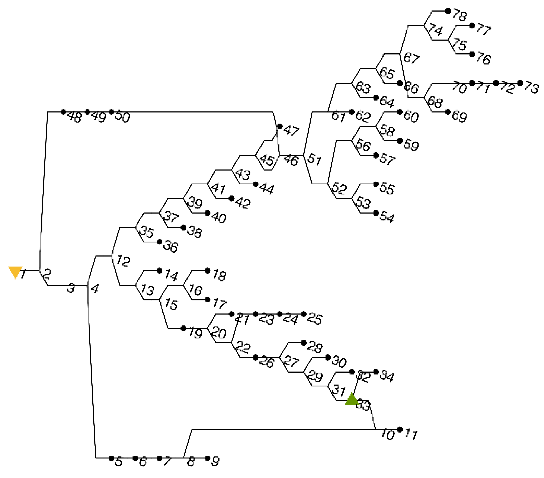
2.1. Gas Network Model Description
| ; | ; |
- b mass flow rates for each pipe;
- n pressures for each node;
- n mass flow rates exchanged with the external environment.
2.2. Conditional Boundary Conditions
2.3. Case Study Description
2.4. Methodology
3. Results
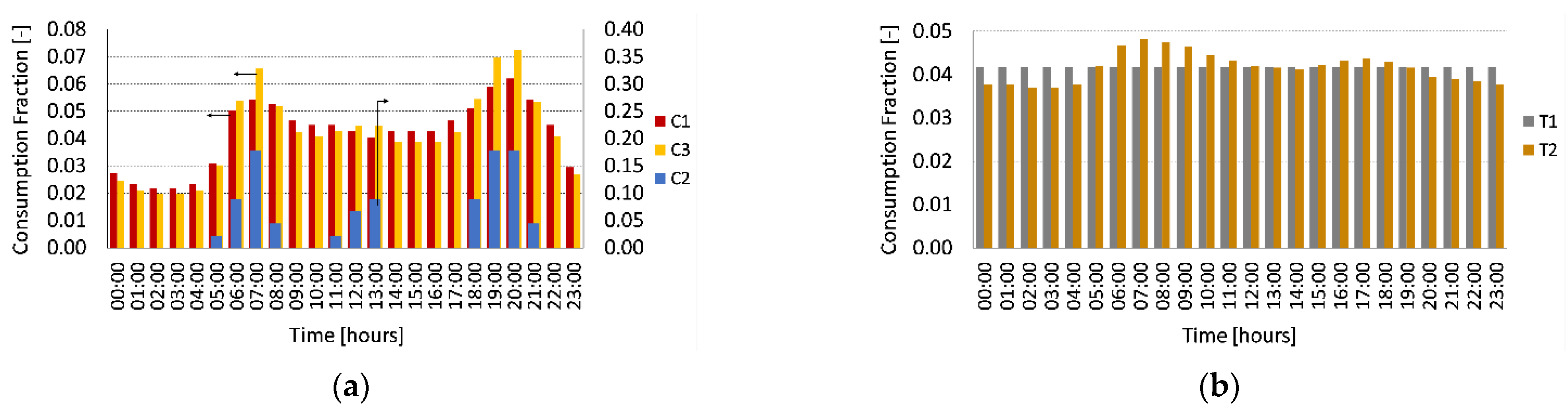
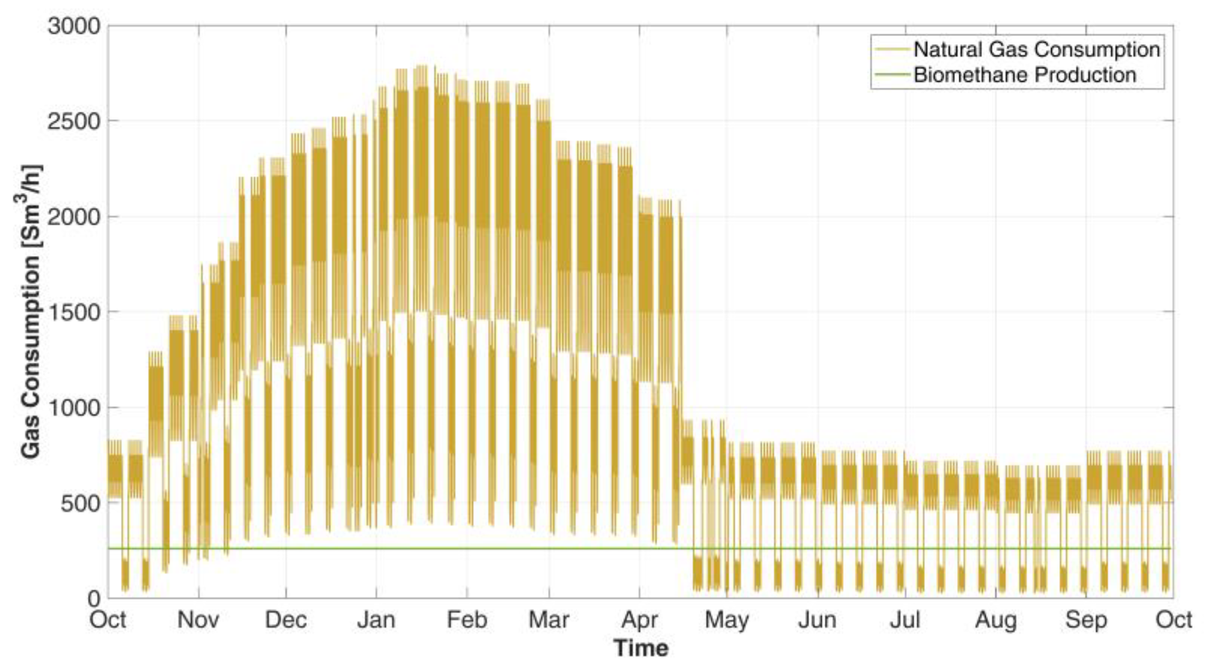
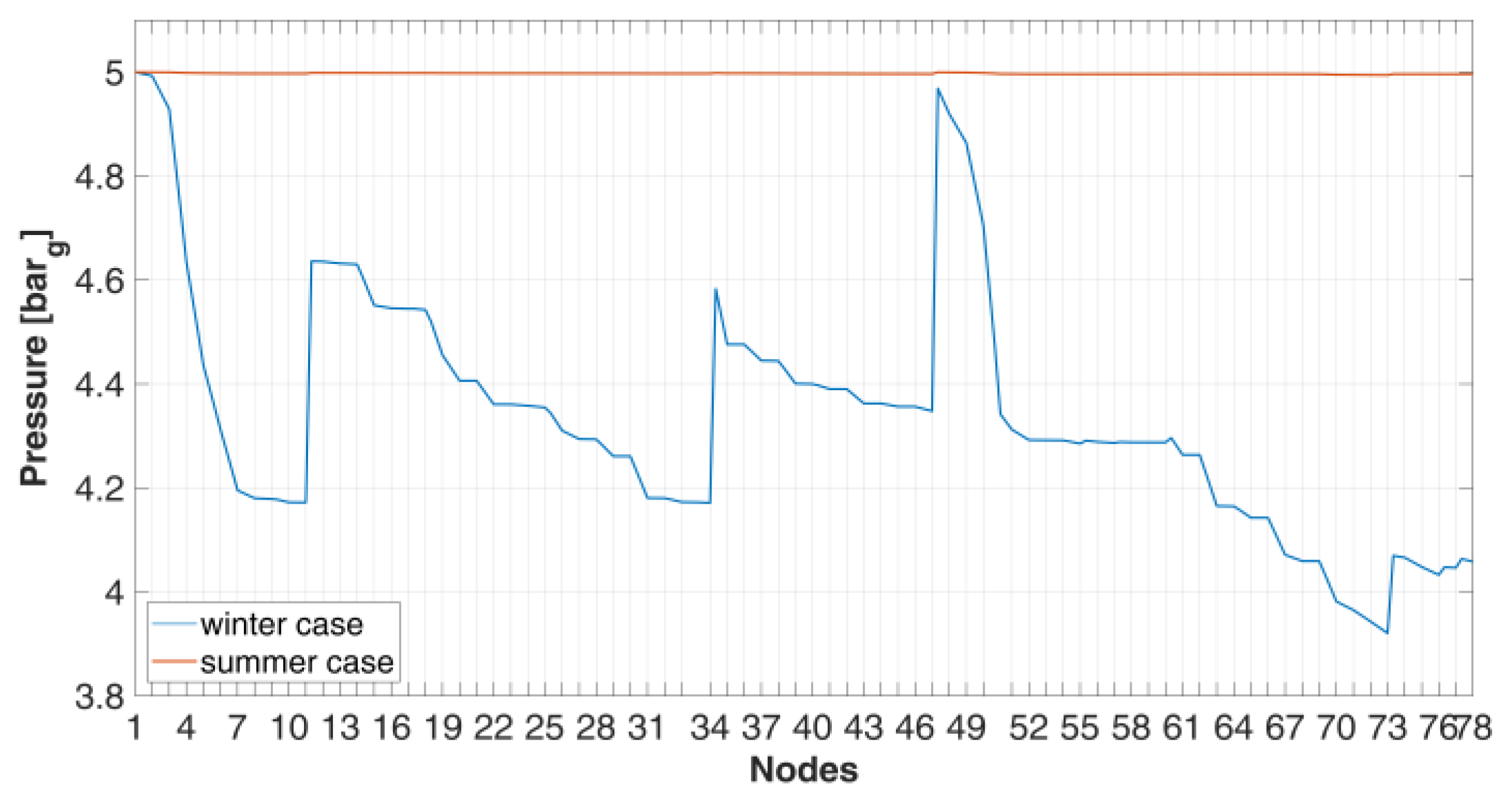
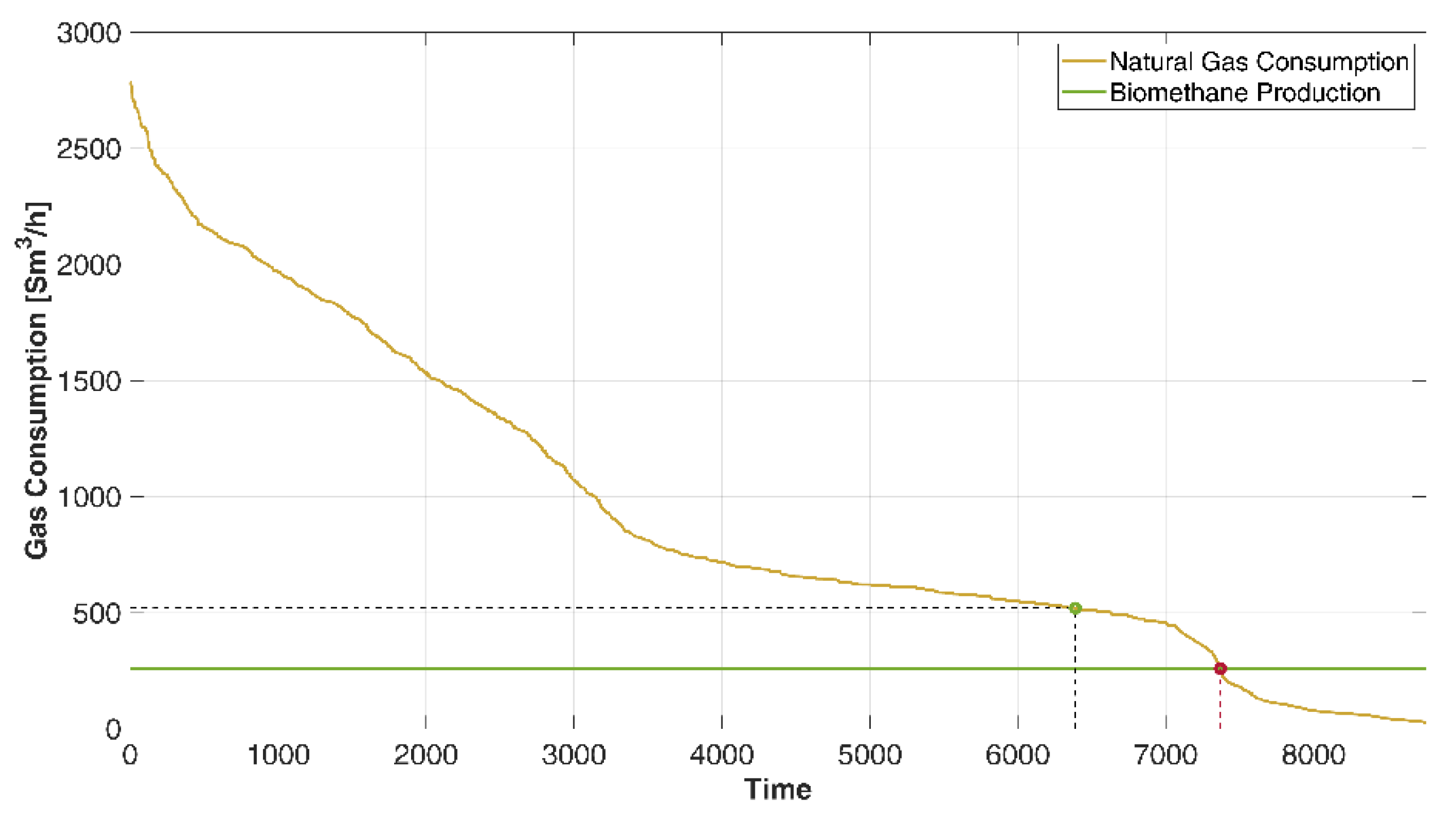
3.1. Preliminary Production-Consumption Analysis
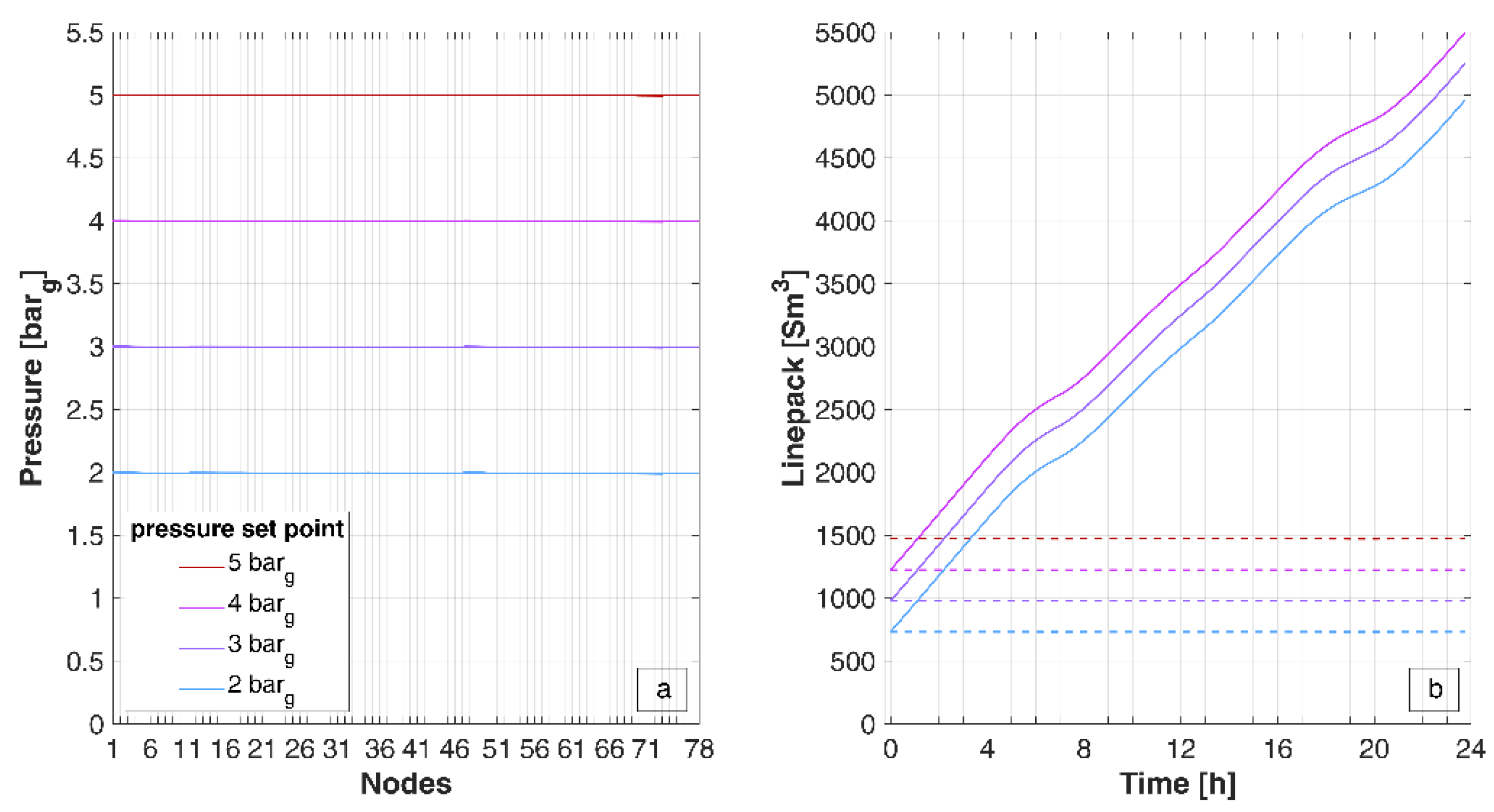
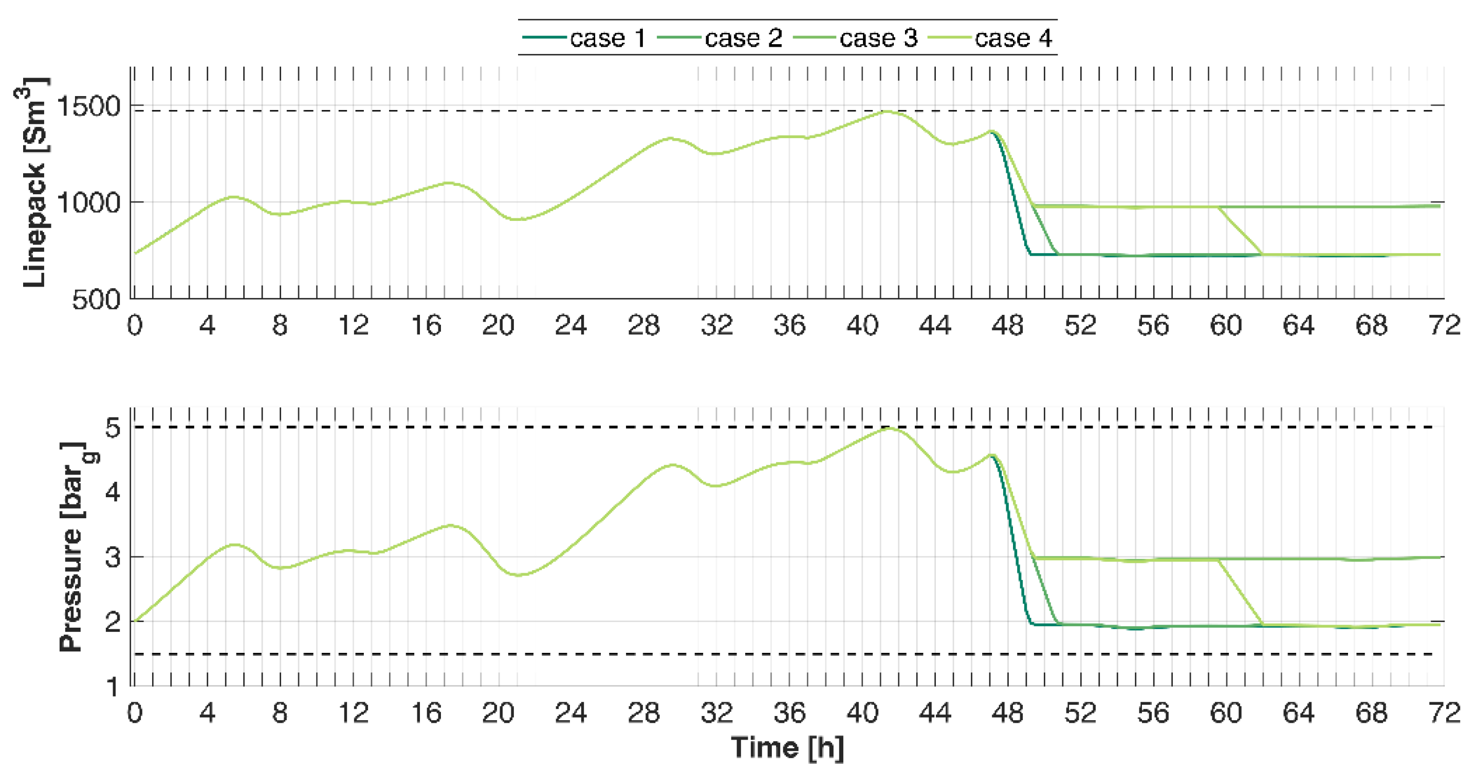
3.2. Unlocking of the Linepack Storage by Pressure Modulation
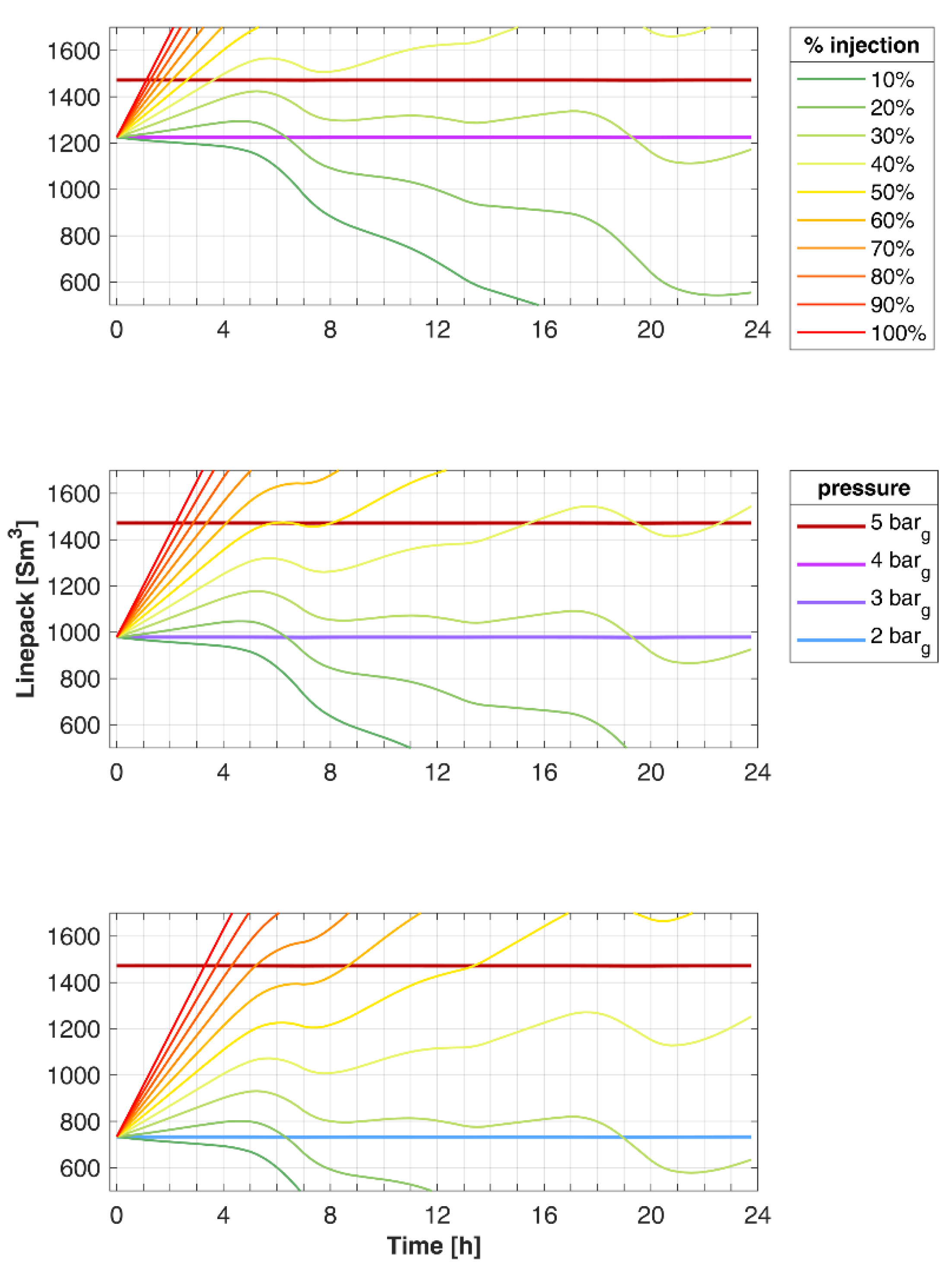
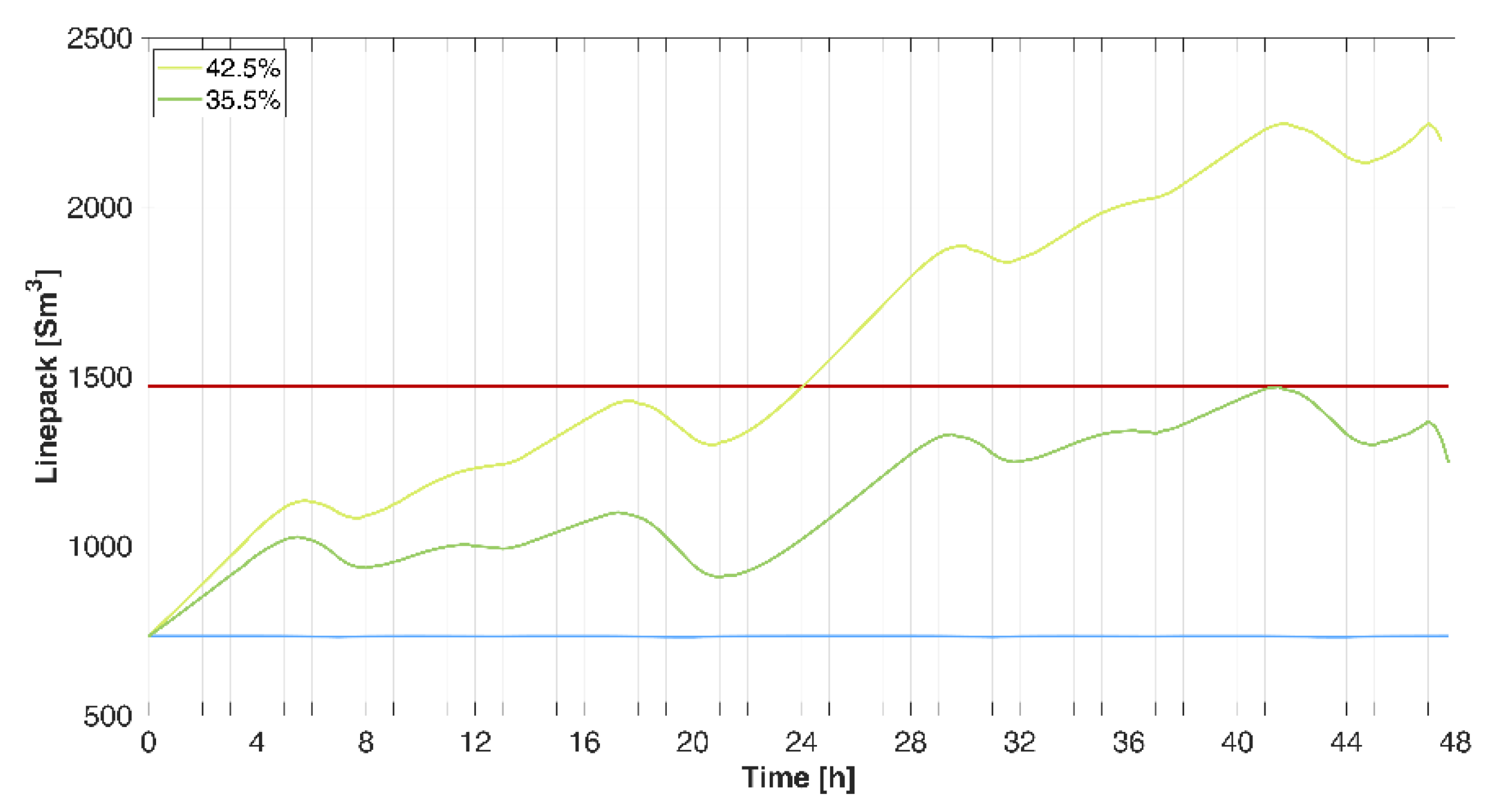
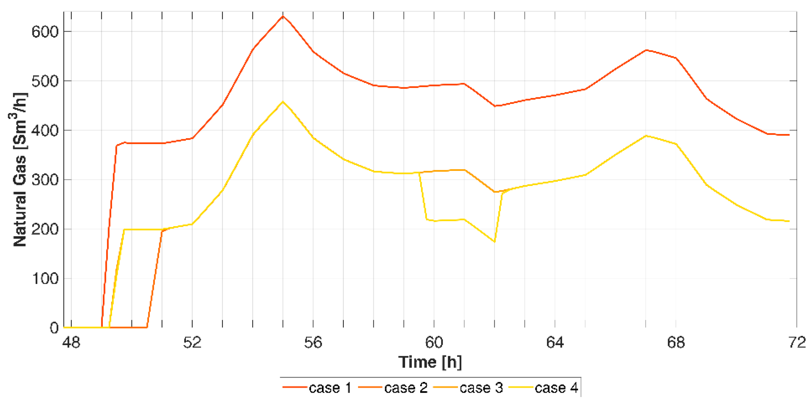
3.3. Biomethane Injection Partialization
4. Discussion
5. Conclusions
Author Contributions
Funding
Data Availability Statement
Conflicts of Interest
References
- European Commission. REPowerEU. Joint European Action for More Affordable, Secure and Sustainable Energy; European Commission: Brussel, Belgium, 2022. [Google Scholar]
- Gas for Climate. Fit for 55 Package and Gas for Climate; Gas for Climate Cosnortium: The Hague, The Netherlands, 2021. [Google Scholar]
- Thrän, D.; Billig, E.; Persson, T.; Svensson, M.; Daniel-Gromke, J.; Ponitka, J.; Seiffert, M. Biomethane Status and Factors Affecting Market Development and Trade; IEA Bioenergy: Paris, France, 2014; ISBN 9781910154106. [Google Scholar]
- Calbry-Muzyka, A.; Madi, H.; Rüsch-Pfund, F.; Gandiglio, M.; Biollaz, S. Biogas Composition from Agricultural Sources and Organic Fraction of Municipal Solid Waste. Renew. Energy 2022, 181, 1000–1007. [Google Scholar] [CrossRef]
- Chiumenti, A.; da Borso, F.; Limina, S. Dry Anaerobic Digestion of Cow Manure and Agricultural Products in a Full-Scale Plant: Efficiency and Comparison with Wet Fermentation. Waste Manag. 2018, 71, 704–710. [Google Scholar] [CrossRef] [PubMed]
- European Biogas Association. EBA Statistical Report 2021; European Biogas Association: Brussels, Belgium, 2021. [Google Scholar]
- Scarlat, N.; Dallemand, J.-F.; Fahl, F. Biogas: Developments and Perspectives in Europe. Renew. Energy 2018, 129, 457–472. [Google Scholar] [CrossRef]
- Italian Ministry of Economic Development. Decreto Interministeriale 18 Dicembre 2008—Incentivi Produzione Energia 2008; Italian Ministry of Economic Development: Roma, Italy, 2008. [Google Scholar]
- GSE. Energia Da Fonti Rinnovabii in Italia—Rapporto Statistico 2017; GSE: Roma, Italy, 2018. [Google Scholar]
- Eurostat Renewable Energy Statistics. Available online: https://ec.europa.eu/eurostat/statistics-explained/index.php/Renewable_energy_statistics (accessed on 28 September 2022).
- Italian Ministry of Economic Development. Decreto Interministeriale 2 Marzo 2018—Promozione Dell’uso Del Biometano Nel Settore Dei Trasporti; Italian Ministry of Economic Development: Roma, Italy, 2018. [Google Scholar]
- GIE; EBA European Biomethane Map. Available online: https://www.europeanbiogas.eu/wp-content/uploads/2020/06/GIE_EBA_BIO_2020_A0_FULL_FINAL.pdf (accessed on 28 September 2022).
- Directorate-General for Energy. Mandate to CEN for Standards for Biomethane for Use in Transport and Injection in Natural Gas Pipelines; European Commission: Brussel, Belgium, 2010. [Google Scholar]
- UNI EN 16723:2016; Gas naturale e Biometano per l’utilizzo nei Trasporti e per l’immissione nelle reti di gas Naturale. Ente Italiano di Normazione: Roma, Italy, 2016.
- UNI/TS 11537:2019; Immissione di Biometano nelle reti di Trasporto e Distribuzione di gas Naturale. Ente Italiano di Normazione: Roma, Italy, 2019.
- Graf, F.; Ortloff, F.; Kolb, T. Biomethane in Germany - Lessons Learned. In Proceedings of the 26th World Gas Conference, Paris, France, 1–5 June 2015; Volume 16, pp. 142–145. [Google Scholar]
- DVGW. DVGW G 265-2:2012-01—Anlagen Für Die Aufbereitung Und Einspeisung von Biogas in Erdgasnetze—Teil 2: Fermentativ Erzeugte Gase—Betrieb Und Instandhaltung; DVGW: Bonn, Germany, 2012. [Google Scholar]
- Quintino, F.M.; Nascimento, N.; Fernandes, E.C. Aspects of Hydrogen and Biomethane Introduction in Natural Gas Infrastructure and Equipment. Hydrogen 2021, 2, 16. [Google Scholar] [CrossRef]
- Stürmer, B. Greening the Gas Grid-Evaluation of the Biomethane Injection Potential from Agricultural Residues in Austria. Processes 2020, 8, 630. [Google Scholar] [CrossRef]
- Pasini, G.; Baccioli, A.; Ferrari, L.; Antonelli, M.; Frigo, S.; Desideri, U. Biomethane Grid Injection or Biomethane Liquefaction: A Technical-Economic Analysis. Biomass Bioenergy 2019, 127, 105264. [Google Scholar] [CrossRef]
- Casasso, A.; Puleo, M.; Panepinto, D.; Zanetti, M. Economic Viability and Greenhouse Gas (Ghg) Budget of the Biomethane Retrofit of Manure-Operated Biogas Plants: A Case Study from Piedmont, Italy. Sustainability 2021, 13, 7979. [Google Scholar] [CrossRef]
- Anigas; Assogas; Utilitalia. Immissione Diretta Di Biometano in Rete; Anigas: Milano, Italy, 2016. [Google Scholar]
- Energinet. Long-Term Development Needs in the Danish Gas System; Energinet: Fredericia, Denmark, 2022. [Google Scholar]
- Agency Danish Environmental Protection Decision to Establish Biogas Pipeline between St. Andst and Pottehuse and a Compressor Station at St. Andst: EIA Is Not Required (in Danish). Available online: https://mst.dk/service/annoncering/annoncearkiv/2017/maj/vvm-screening-biogasledning-ml-st-andst-og-pottehuse/ (accessed on 14 April 2020).
- Cavana, M.; Leone, P. Biogas Blending into the Gas Grid of a Small Municipality for the Decarbonization of the Heating Sector. Biomass Bioenergy 2019, 127, 105295. [Google Scholar] [CrossRef]
- Osiadacz, A.J.; Chaczykowski, M. Comparison of Isothermal and Non-Isothermal Pipeline Gas Flow Models. Chem. Eng. J. 2001, 81, 41–51. [Google Scholar] [CrossRef]
- Abeysekera, M.; Wu, J.; Jenkins, N.; Rees, M. Steady State Analysis of Gas Networks with Distributed Injection of Alternative Gas. Appl. Energy 2015, 164, 991–1002. [Google Scholar] [CrossRef]
- Chaudry, M.; Jenkins, N.; Strbac, G. Multi-Time Period Combined Gas and Electricity Network Optimisation. Electr. Power Syst. Res. 2008, 78, 1265–1279. [Google Scholar] [CrossRef]
- Cheng, N.S. Formulas for Friction Factor in Transitional Regimes. J. Hydraul. Eng. 2008, 134, 1357–1362. [Google Scholar] [CrossRef]
- Kunz, O.; Wagner, W. The GERG-2008 Wide-Range Equation of State for Natural Gases and Other Mixtures: An Expansion of GERG-2004. J. Chem. Eng. Data 2012, 57, 3032–3091. [Google Scholar] [CrossRef]
- Cavana, M.; Leone, P. Solar Hydrogen from North Africa to Europe through Greenstream: A Simulation-Based Analysis of Blending Scenarios and Production Plant Sizing. Int. J. Hydrogen Energy 2021, 46, 22618–22637. [Google Scholar] [CrossRef]
- ARERA. 229/2012/R/GAS—Testo Integrato Delle Disposizioni Dell’Autorità per l’energia Elettrica e Il Gas in Ordine Alla Regolazione Delle Partite Fisiche Ed Economiche Del Servizio Di Bilanciamento Del Gas Naturale (Settlement); ARERA: Roma, Italy, 2012. [Google Scholar]
- European Parliament and the council of the European Union. Directive 2004/22/EC of the European Parliament and of the Council of 31 March 2004 on Measuring Instruments; European Parliament: Strasbourg, France, 2004. [Google Scholar]


| Control Mode | Equation | Coefficients |
|---|---|---|
| pressure | ||
| mass flow | ||
| junction/no flow |
| Code | Description | Seasonality |
|---|---|---|
| C1 | Space heating | yes |
| C2 | Cooking and/or DHW | no |
| C3 | Space heating + cooking and/or DHW | yes |
| T1 | Technological use | no |
| T2 | Technological + space heating | yes |
| Code | Withdrawal Days |
|---|---|
| 1 | 7 days per week |
| 2 | 6 days per week (excluding Sundays and national holidays) |
| 3 | 5 days per week (excluding Saturdays, Sundays, and national holidays) |
| Pressure Set Point | 4 barg | 3 barg | 2 barg |
|---|---|---|---|
| Saturation time | 1 h 7′ | 2 h 12′ | 3 h 18′ |
| Accumulation capacity | 247 Sm3/h | 493.3 Sm3/h | 738.6 Sm3/h |
| Curtailment Criteria | Yearly Injection (MSm3) | # Hours | % | % of Biomethane Curtailment |
|---|---|---|---|---|
| strict | 1.66 | 6389 | 72.9 | 27.1 |
| loose | 1.91 | 7369 | 84.1 | 15.9 |
| with pressure and injection management | 2.05 | 7852.8 * | 89.6 | 10.4 |
Publisher’s Note: MDPI stays neutral with regard to jurisdictional claims in published maps and institutional affiliations. |
© 2022 by the authors. Licensee MDPI, Basel, Switzerland. This article is an open access article distributed under the terms and conditions of the Creative Commons Attribution (CC BY) license (https://creativecommons.org/licenses/by/4.0/).
Share and Cite
Cavana, M.; Leone, P. Smart Gas Network with Linepack Managing to Increase Biomethane Injection at the Distribution Level. Energies 2022, 15, 8198. https://doi.org/10.3390/en15218198
Cavana M, Leone P. Smart Gas Network with Linepack Managing to Increase Biomethane Injection at the Distribution Level. Energies. 2022; 15(21):8198. https://doi.org/10.3390/en15218198
Chicago/Turabian StyleCavana, Marco, and Pierluigi Leone. 2022. "Smart Gas Network with Linepack Managing to Increase Biomethane Injection at the Distribution Level" Energies 15, no. 21: 8198. https://doi.org/10.3390/en15218198
APA StyleCavana, M., & Leone, P. (2022). Smart Gas Network with Linepack Managing to Increase Biomethane Injection at the Distribution Level. Energies, 15(21), 8198. https://doi.org/10.3390/en15218198