Article

Improved Semi-Supervised Data-Mining-Based Schemes for Fault Detection in a Grid-Connected Photovoltaic System

1
LESM Lab., Faculty of Technology, University of Saida-Dr Moulay Tahar, Saida 20000, Algeria
2
STIC Lab., Department of Telecommunications, Abou Bekr Belkaid University, Tlemcen 13000, Algeria
3
Computer, Electrical and Mathematical Sciences and Engineering (CEMSE) Division, King Abdullah University of Science and Technology (KAUST), Thuwal 23955-6900, Saudi Arabia
4
Centre de Développement des Energies Renouvelables (CDER), B.P. 62, Route de l’Observatoire, Algiers 16340, Algeria
5
Laboratoire de Dispositifs de Communication et de Conversion Photovoltaique, Ecole Nationale Polytechnique Alger, Algiers 16200, Algeria
*
Author to whom correspondence should be addressed.
Energies 2022, 15(21), 7978; https://doi.org/10.3390/en15217978
Submission received: 5 October 2022 / Revised: 21 October 2022 / Accepted: 24 October 2022 / Published: 27 October 2022

Abstract

:
Fault detection is a necessary component to perform ongoing monitoring of photovoltaic plants and helps in their safety, maintainability, and productivity with the desired performance. In this study, an innovative technique is introduced by amalgamating Latent Variable Regression (LVR) methods, namely Principal Component Regression (PCR) and Partial Least Square (PLS), and the Triple Exponentially Weighted Moving Average (TEWMA) statistical monitoring scheme. The TEWMA scheme is known for its sensitivity to uncovering changes of small magnitude. Nevertheless, TEWMA can only be utilized for monitoring single variables and ignoring the correlation among monitored variables. To alleviate this difficulty, the LVR methods (i.e., PCR and PLS) are used as residual generators. Then, the TEWMA is applied to the obtained residuals for fault detection purposes, where the detection threshold is computed via kernel density estimation to improve its performance and widen its applicability in practice. Real data with different fault scenarios from a 9.54 kW photovoltaic plant has been used to verify the efficiency of the proposed schemes. Results revealed the superior performance of the PLS-TEWMA chart compared to the PLS-TEWMA chart, particularly in detecting anomalies with small changes. Moreover, they have almost comparable performance for large anomalies.

1. Introduction

The energy supply of the future must be clean, efficient, resource-efficient, and sustainable. Solar Photovoltaic (PV) energy is a strategic option to satisfy environmental concerns and meet the growing electricity demand [1]. It offers a safe, affordable, and renewable solution for generating power on a large scale. The latest statistics show that the installed PV systems reached a total installed capacity of 942 GWdc (Gigawatt direct current) in 2021 [2]. Although there are advanced PV technologies, PV systems are still confronted with different types of anomalies in real working conditions, such as short-circuit, open-circuit, line-line, and partial shading, that decrease their performance and cause power losses [3]. Undoubtedly, such unsatisfactory faulty conditions raise undesirable maintenance costs and inefficiency.
Anomalies and atypical conditions (e.g., dirt, shading) can make the PV system deviate from the desired performance. Broadly speaking, both internal and external anomalies in PV systems can degrade their operating performance, collapsing the system and even resulting in severe security issues [4]. Internal faults include line-to-line faults, short/open circuits, and defective components (e.g., generators, cables, and inverters). In addition, external anomalies are related to some environmental circumstances, like dusty conditions [5], and subversive acts, such as cyber-attacks (e.g., Denial of services and data integrity), particularly against on-grid plants [6,7,8]. In the absence of convenient action, the system lifetime can be drastically reduced in the long term [9]. Thus, PV systems need to be continuously monitored for proper functioning, preserving their optimal performances and making them more efficient, reliable, and sustainable [10].
Detecting anomalies in PV systems is essential to avoid energy drops and keep their expected performance. Towards this end, numerous anomaly detection techniques have been developed in the literature last two decades. Such techniques can be grouped into two principal classes, namely, model-based or data-driven methods [11,12,13,14,15,16,17]. Model-based approaches involve analytical models to predict normal (i.e., fault-free) PV system outputs. Abnormal measurements are flagged when their deviations from the predictions exceed the set threshold [13,16,17]. Various model-based approaches have been introduced in the literature, such as single-diode-based models [18], double-diode-based models [19], and Kalman filter [20]. For instance, Skomedal et al. [21] compared six monitoring charts, the conventional Shewhart, three modified versions of CUSUM (Cumulative Sum), and a modified modification of EWMA (Exponentially Weighted Moving Average), based on an autoregressive integrated moving average model to detect low-rate losses in sizable grand serial PV farms. They conclude that the best performance is obtained when using CUSUM-based charts in this application. In [18], an approach to detect and identify faults in the DC side of a PV plant is presented. This approach applies the Multivariate EWMA to residuals obtained from the one-diode-based model for fault detection and the univariate EWMA to residuals to discriminate the types of detected anomalies. Of course, the efficiency of the model-based anomaly detection methods depends on the analytical model, which is not often easy to obtain and time-consuming, particularly for large-scale systems.
Data-driven approaches, on the other hand, exploit available measurements when the monitored PV system is functioning properly to learn the underlying reference empirical model. Then, new faulty measurements are uncovered accordingly [22,23,24]. Data-based anomaly detection techniques enclose statistical and machine learning-based techniques, e.g., Support Vector Machine (SVM) and k-Nearest Neighbors (k-NN) algorithm. Within data-based techniques, in [25], an approach based on Principal Component Analysis (PCA) is proposed to monitor the DC side of a PV system. More specifically, PCA is applied to select the most relevant features and generate residuals. Here, residuals are evaluated via the multivariate charts Hotelling T2 and Squared Predicted Error (SPE) charts for anomaly detection purposes. This approach showed satisfactory detection performance in detecting different real anomalies, including short-circuit, inverter connection, and partial shading. In [26], the PCA approach showed performance in detecting and classifying PV shading under real conditions. In another study [27], a PCA-based image processing method was introduced to detect faults in PV tracking systems. Deceglie et al. [28] proposed the Stochastic Rate and Recovery (SRR) approach to compute losses related to the soiling problem. The SRR defines cleaning and soiling periods using short-circuit current measurements. Then soiling ratios are used to discriminate soiling profiles, and the resulting losses are estimated according to prefixed cleaning thresholds. This study revealed that profile construction is very sensitive to noise, and the estimation threshold should be judiciously set. In [29], Kilic et al. addressed open and short circuit-related failures with the Random Vector Functional Link Networks (RVFLN) and Canonical Correlation Analysis (CCA) as data reduction techniques to reduce the dimension of selected attributes.
In [30], Xiong et al. studied the utility of Discrete Wavelet Transform (DWT) to identify and isolate parallel and series arc faults. Specifically, the DWT-based technique is applied to inspect capacitor current features, and results show significant variations during arc faults, which allow for the revealing of their type and location. Nevertheless, the analysis is based on simplified alleged data and specific arc faults. Indeed, it should be generalized for other fault types onboard real PV systems. The approach proposed in [31] employs Wavelets Packet Transform (WPT). Here, three PV plant’s variables have been chosen to perform de detection procedure: voltage, voltage/energy, and impedance/energy. For each variable, preset thresholds obtained through simulation are used to define the intervals of normal variations. In [32], Edun et al. presented a method to detect disconnections in PV systems using the Spread Spectrum Time Domain Reflectometry (SSTDR). It consists of correlating generated to reflected signals, and the obtained baseline peaks are utilized to reveal and locate the related faults. However, the SSTDR is too sensitive to noise and attenuation, making it relatively adapted to a limited number of cells. In addition, the use of this approach gets more complicated in large-scale PV plants where a large number of reflections can strongly degrade their detection performance.
Recently, several supervised and semi-unsupervised machine leaning-based techniques have been explored for fault detection and classification in PV systems [33,34,35,36]. Supervised methods require the availability of labeled data during the training, which is not often easy to obtain, particularly for large-scale systems with various faults. On the other hand, semi-supervised methods need only fault-free data in training and without fault labeling. In [37], individual modules’ voltages are estimated by means of multi-layer neural networks to find out short circuit situations. Results showed that detection accuracy increased proportionally with the number of used layers. However, the training of this model requires faulty measurements, which is not always feasible, even if it does not cover all expected faults. Chen et al. [38] presented a multi faults detection approach based on enhanced Semi-Supervised Ladder Networks (SSLN) when using restricted online samples. In [39], an auto-encoder-driven deep neural network approach is designed to deal with operational and cyber-attacks related faults in grid-connected PV systems. The auto-encoder is applied to estimate the normal measurements with the lowest error based on multivariate features. Then faults are reported when estimation error exceeds an empirical detection threshold based on the well-known three-sigma rule. In [40], the SVM algorithm is applied to quantify power quality and isolate eventual disturbances within client-side measurements. First, the DWT selects and extracts the most relevant features. Next, the One-Class SVM (OCSVM) is involved in revealing disturbances. Finally, a Multi-Class SVM (MCSVM) procedure is performed to classify the detected disturbances.
Anomaly detection in PV plants is essential for improving their safety and profitability and optimizing maintenance scheduling. Possible anomalies could be caused by malfunctioning sensors (sensor anomalies) or changes affecting the inspected system (called process anomalies). The need for methods to accurately and quickly uncover abnormal conditions (sensor or process anomalies) is vital to keep the PV system operating with the desired performance. This paper presents a data-driven approach for detecting sensor anomalies and anomalies in the DC side of the PV system. Importantly, the aim is to develop a semi-supervised data-driven detector for PV systems monitoring that does not require labeled data. In this study, we propose a Triple Exponentially Weighted Moving Average (TEWMA)-based strategy to detect anomalies encountered in the DC side of a PV plant. The TEWMA scheme is an effective and sensitive approach, which is found to have better detection of small changes, usually adopted for inspecting only single process variables. However, data from PV systems are multivariate input-output variables and cross-correlated, making the use of the TEWMA chart inappropriate. To bypass this shortcoming, the proposed method integrates Latent Variable Regression (LVR) methods with the TEWMA chart. LVR models, namely, Principal Component Regression (PCR) and Partial Least Square Regression (PLS), demonstrated good capability in modeling multivariate input-output data in different applications by eliminating variables’ collinearity and reducing noises as well. In addition, PLS/PCR models have been widely employed for response variables prediction based on predictor variables. They perform well when transforming high dimensional input data to lower dimension outputs that can be effectively used to track abnormal situations. Importantly, the proposed LVR-TEWMA approach employs two complementary steps in detecting anomalies. The first involves the use of the LVR models (i.e., PLS and PCR) to generate the residual sequence and the TEWMA decision threshold based on data from the PV system under nominal conditions. In the second step, the TEWMA charting statistic is computed using residuals from the reference LVR model based on the newly received data. Comparison of the TEWMA statistic to the determined threshold value yields the anomaly decision (faulty or healthy conditions). Note that the threshold in the conventional TEWMA chart is analytically determined based on the Gaussian assumption of the data distribution. However, this assumption is not valid for the data from PV systems. Here, we extend the TEWMA chart to monitor non-Gaussian data by using the Kernel density estimator to determine the detection threshold.
This work is organized as follows. Section 2 is devoted to the description of the used grid-tied PV system. Then, Section 3 presents the LVR models (i.e., PLS and PCR) for PV system modeling. Section 4 briefly describes the proposed LVR-TEWMA monitoring method and discusses the experimental results. The last section includes this study and provides some future directions.

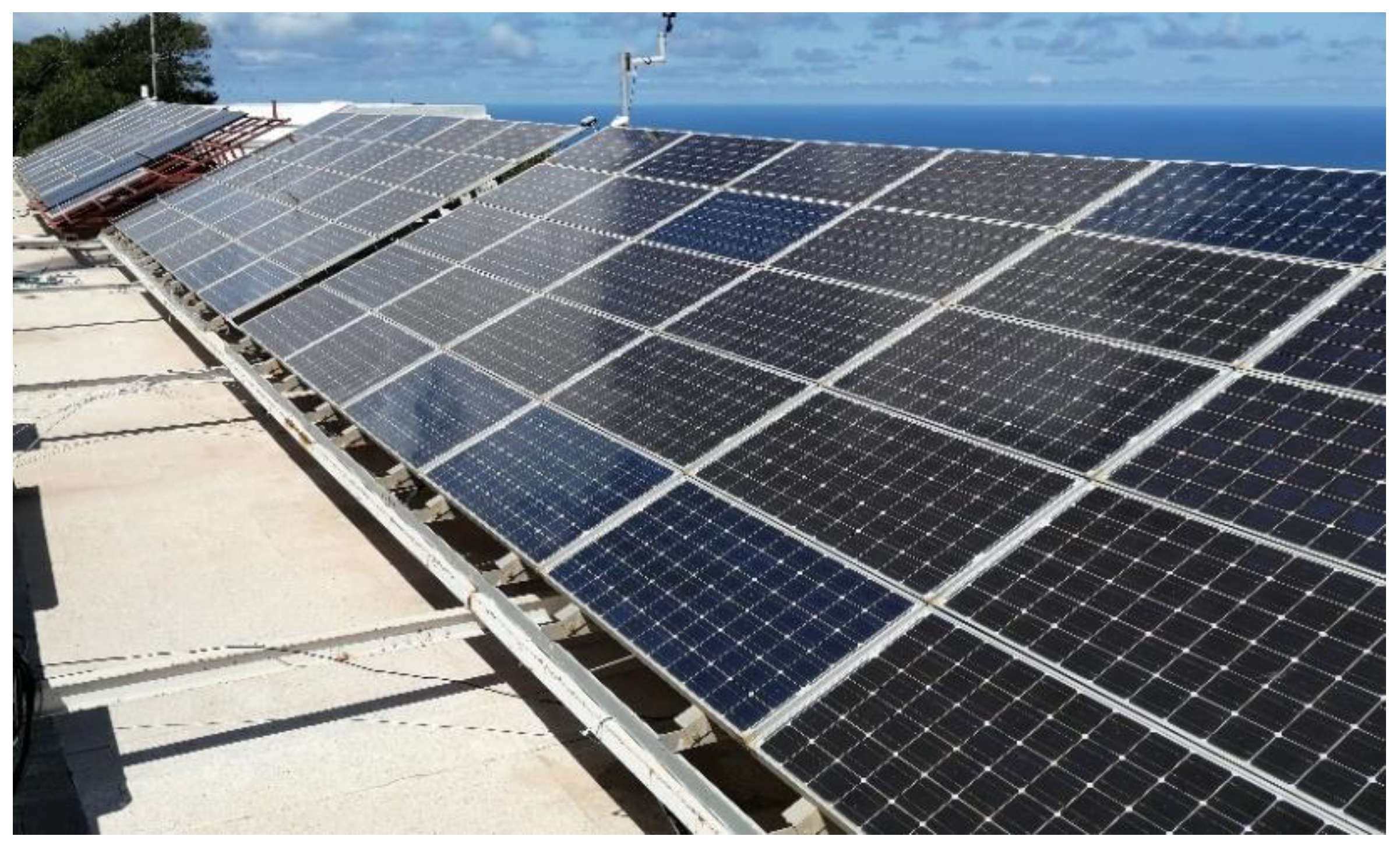
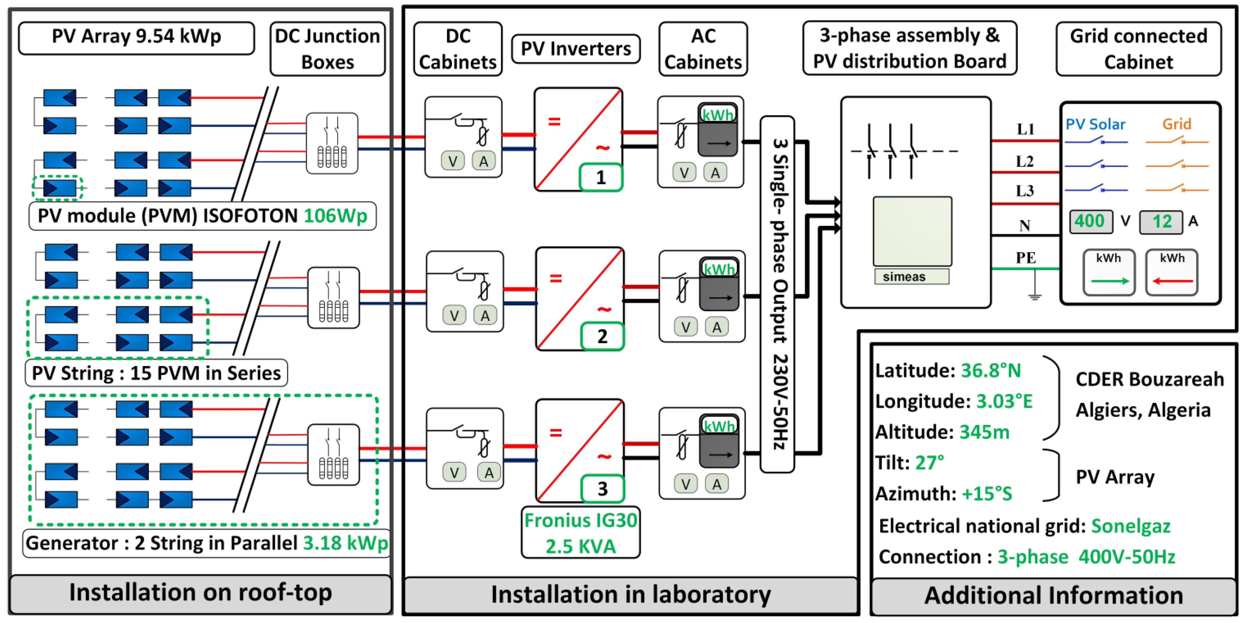
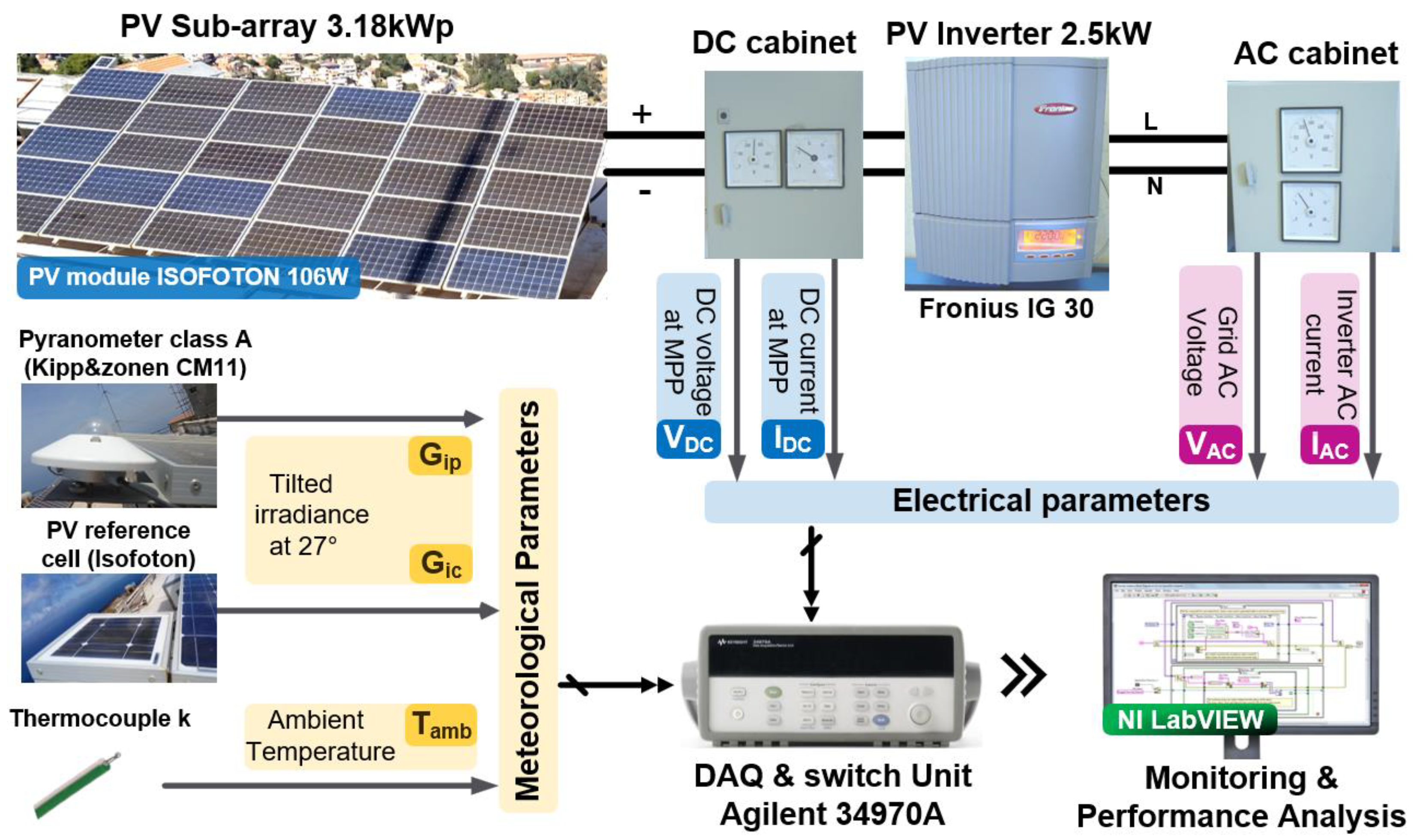
2. PV Installation Description

This section is devoted to presenting shortly the Grid-Connected Photovoltaic (GCPV) installation used in this study. Indeed, the proposed fault detection algorithm in this work will be verified using the meteorological and electrical data measurement collected from a PV installation at the Centre de Developpement des Energies Renouvelables (CDER) in Algeria, with a total power of 9.54 kWdc in operation since 2004 (Figure 1), where the total solar PV power produced is injected into the low-voltage electrical grid. As shown in Figure 2, the PV system is composed of three identical single-phase PV sub-systems. Each PV sub-system contains a PV sub-array of 30 PV Modules (PVM), a 2.5-kilowatt (kW) grid-tie inverter, and electrical cabinets for protection.
The PV array is divided into three sub-arrays. Each PV sub-array contains two parallel strings of 15 PVM in a series. The main electrical specifications of the PV Modules/sub-array and the grid-tie inverter are shown respectively in Table 1 and Table 2.
Where STC symbolizes the Standard Test Conditions (G = 1000 W/m2, TC = 25 °C, and AM = 1.5) and MPP symbolizes the Maximum Power Point. G is the received Irradiance by the PV module during the flash test, TC is the temperature of the PV Cell, and AM is the Air Mass. ISC is the short circuit current, VOC is the open circuit voltage, IMPP is the current at MPP, VMPP is the voltage at MPP, and PM is the maximum power.
The meteorological and electrical measured data used in this work are recovered by an external monitoring system composed essentially of Sensors, a Data Acquisition unit (Agilent 34970A), and software under PC (Figure 3).
For the measure of tilted irradiance at 27 °C, a pyranometer (kipp&zonen CM11) and a reference cell are used, and a thermocouple measures the ambient temperature. Two hall-effect sensors (FW BELL CLSM-50S) were used to measure the current on both the Direct current (DC) and Alternating Current (AC) sides of the grid-tied inverter. The DC voltage at the MPP of the PV sub-array is measured by a simple voltage divider circuit; on the other hand, a voltage transformer was used to measure the grid AC voltage.
The data acquisition and switch unit (Agilent 34970A) provides conditioning and measurement of sensor signals. While the monitoring interface is designed under LabVIEW software, this interface can recover, display, record, and analyze the measured data. According to IEC 61724 standard, the sampling time was chosen at 1 min.

3. Materials and Methods

Here, we briefly introduce the KDE-Triple EWMA approach, PCR, and PLS-based anomaly detection schemes.

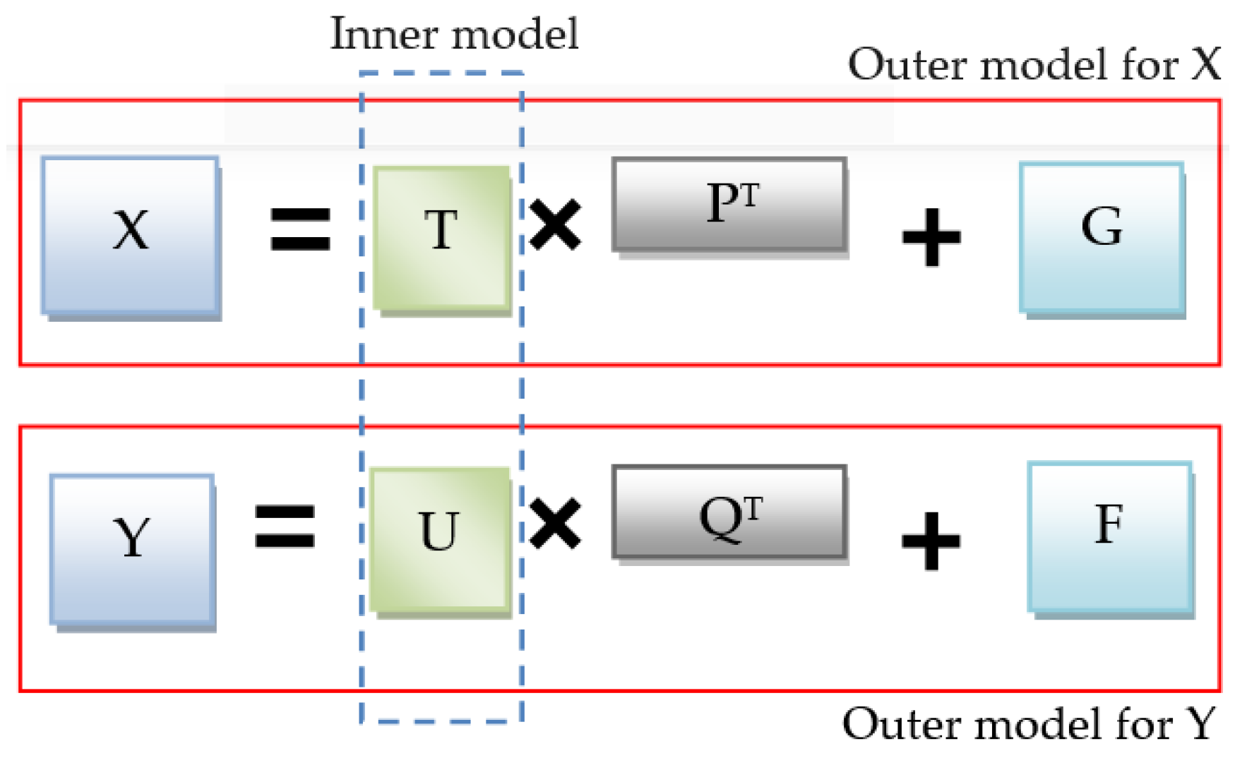
3.1. PLS (Partial Least Square)

PLS, also called Projection to Latent Structures, is a well-known data-driven dimensionality reduction technique that has been extensively applied to monitor multivariate and highly correlated variables [41,42,43,44]. The essence of PLS model consists of transforming input and output data into a lower dimension space so that their corresponding latent variables have the maximum variance [43,44]. Importantly, PLS constructs a model linking the latent variables (LVs) associated with X and Y. The PLS model comprises two complementary models: inner and outer models (Figure 4).
Specifically, for data inputs X with n observations from m variables, X R n × m and data output Y with n observations from p variables, Y R n × p , the PLS model (i.e., outer model) can be expressed as follows [42,45]:
{ X = i = 1 l tp i T = TP t + G Y = i = 1 l uq i T = UQ t + F ,
where T R n × l and U R n × q represent the latent variable matrices associated with input and output matrices, respectively. The loading matrices of input and output space are P R m × l and Q R p × q , respectively. G and F represent the PLS model residuals matrices. Here, l is the number of retained principal components (PCs), which can be calculated using the cross-validation method [46]. The retained latent variables u j and t j are estimated iteratively [47], and the PLS model establishes the relationship (i.e., inner model) between T and U as:
U = T β + E ,  
where β denotes the regression matrix and E is the residual matrix. Finally, the output variable Y is obtained via the following expression:
Y = T β Q T + F *
Various extensions to the linear PLS model have been reported in the literature to widen the applicability of PLS models in practice, including nonlinear PLS [41], wavelet-driven PLS [48], recursive PLS [49], and dynamic PLS [50].

3.2. PCR (Principal Component Regression)

We now describe the PCR model. The PCR method is frequently used in dimensionality reduction and regression to handle the collinearity problem in multivariate data. PCR is performed in two complementary phases. At first, the data reduction procedure is applied to explanatory variables X using Principal component analysis (PCA). After that, the resulting retained principal components (CPs) are then linked to the response variables via the Ordinary Least Squares (OLS) regression technique [51,52] (Figure 5).
After applying the PCA algorithm, the input data matrix X is decomposed as follows [52]:
X = T W T = i = 1 k t i w i T + i = K + 1 m t i w i T = X ^ + E ,
where X ^ , and E are the approximated and residual matrices, respectively. Here, T R n × m and W R m × m represent the principal components (PCs) and the loading matrices, respectively. Notice that the cumulative percentage variance (CPV) technique is widely employed to decide the number of PCs to be retained in the model [53]. Therefore, PCR constructs the linear regression between the matrix T ^ of the k retained principal components and the response variable y as the solution for the following optimization problem:
β ^ = arg   min β ( T ^ β y 2 2 ) .
The least squares solution is obtained as:
β ^ = ( T ^ T T ^ ) 1 T ^ T y .
More details about PCR and PLS-driven anomaly techniques can be found in [45].

3.3. TEWMA (Triple Exponential Weighted Moving Average)

The TEWMA (i.e., Triple EWMA) is an enhanced variant of the conventional single EWMA monitoring approach, built essentially for conveniently uncovering changes with small and moderate levels. Precisely, the decision statistic is based on applying triple EWMA of the actual and past data points [54,55]. For a given monitored variable X x i ,   i = 1 , n , samples normally distributed follow normal distribution N ( μ , σ 2 ) , the single EWMA statistic Ei is defined as:
E i = λ 1 x i + ( 1 λ 1 ) E i 1 .
Then the double EWMA statistic, DEi, is expressed as:
DE i = λ 2 E i + ( 1 λ 2 ) DE i 1 .
Finally, the Triple TEWMA statistic, TEi can be calculated as follow:
TE i = λ 3 DE i + ( 1 λ 3 ) TE i 1 .
The smoothing parameters λ1, λ2, and λ3 can either be equal or different. It has been shown that the Double EWMA (DEWMA) maintains mostly the same performance for the same or different smooth parameters [56,57]. The TEWMA charting statistic with the same smoothing parameter is rewritten as follows [54,58]:
{ E i = λ x i + ( 1 λ ) E i 1 ,                                                             DE i = λ E i + ( 1 λ ) DE i 1   ,                                       TE i = λ DE i + ( 1 λ ) ,                                                  
where E 0 = DE 0 = TE 0 = μ 0 initialize the three statistics and usually set to be the anomaly-free mean. As a weighted average, statistic Ei can be written as [54,58]:
E i = λ x i + ( 1 λ ) E i 1 = λ x i + ( 1 λ ) [ λ x i 1 + ( 1 λ ) E i 2 ]                                           = λ [ x i + ( 1 λ ) x i 1 ] +   ( 1 λ ) 2 E i 2 .        
Hereby, the Ei statistic of the present sample can be computed as pondered sum function of all paste samples j [54,56]:
E i = λ j = 1 i ( 1     λ ) i j x j +   ( 1     λ ) i E 0 ,    
Similarly, DEi and TEi can be written as [54,56]:
DE i   = λ j = 1 i ( 1 λ ) i j E j +   ( 1 λ ) i DE 0 ,  
TE i = λ j = 1 i ( 1 λ ) i j DE j + ( 1 λ ) i TE 0 .
After replacing Ei in Equation (13), DEi can be expressed in terms of xi as:
DE i = λ j = 1 i ( 1 λ ) i j [ λ k = 1 j ( 1 λ ) j k x k + ( 1 λ ) j E 0 ] + ( 1 λ ) i DE 0       = λ 2 j = 1 i k = 1 j ( 1 λ ) i k x k + λ j = 1 i ( 1 λ ) i E 0 + ( 1 λ ) i DE 0         = λ 2 k = 1 i j = k i ( 1 λ ) i k x k + λ i ( 1 λ ) i E 0 +   ( 1 λ ) i DE 0 .        
We now substitute E0 into DE0 to obtain the final pondered form [54]:
DE i = λ 2 k = 1 i ( 1 λ ) i k ( i k + 1 ) x k + ( λ i + 1 ) ( 1 λ ) i DE 0
After that, by substituting (16) in (14), TEi is expressed as [54]:
TE i = λ j = 1 i ( 1 λ ) i j [ λ 2 k = 1 j ( 1 λ ) j k ( j k + 1 ) x k + ( λ j + 1 ) ( 1 λ ) j DE 0 ] + ( 1 λ ) i TE 0 = λ 3 j = 1 i k = 1 j ( 1 λ ) i k ( j k + 1 ) x k + λ j = 1 i ( 1 λ ) i ( λ j + 1 ) DE 0 + ( 1 λ ) i TE 0 = λ 3 k = 1 i j = k i ( 1 λ ) i k ( j k + 1 ) x k + λ j = 1 i ( 1 λ ) i ( λ j + 1 ) DE 0 + ( 1 λ ) i TE 0 = λ 3 2 k = 1 i ( 1 λ ) i k ( i k + 1 ) ( i k + 2 ) x k + ( λ 2 ) ( 1 λ ) i i ( λ i + λ + 2 ) DE 0 + ( 1 λ ) i TE 0
Finally, we substitute DE0 into TE0, to obtain the TEi statistic as:
TE i = λ 3 2 k = 1 i ( 1 λ ) i k ( i k + 1 ) ( i k + 2 ) x k + ( ( 1 λ ) i 2 ) [ λ i ( λ i + λ + 2 ) + 2 ] TE 0 .  
The monitoring scheme utilizing TEWMA defines the upper and lower control limits as [54]:
UCL , LCL = μ 0   ±   L σ 6 ( 1 λ ) 6 λ ( 2 λ ) 5 + 12 ( 1 λ ) 4 λ 2 ( 2 λ ) 4 + 7 ( 1 λ ) 2 λ 3 ( 2 λ ) 3 + λ 4 ( 2 λ ) 2 ,  
where TEi values below the limits indicate that the monitored system operates without anomalies. On the other hand, anomalies can be identified when TEi values overpass the defined decision limits.
Note that the decision limits in (19) are calculated under the normality distribution assumption of data. Nevertheless, this is not often satisfied, which could result in increased false alarms rate and missed detections. To overcome this problem, kernel density estimation (KDE) is adopted in this study to compute the decision limit.

3.4. KDE-TEWMA (Kernel Density Estimation TEWMA)

In this section, we introduce KDE, which is commonly used to estimate the probability distribution of a given data, and how it can be used to compute the TEWMA threshold. Let us consider X = x 1 ; ; x n represents the residual vector using PLS or PCR model. The KDE is applied for estimating the probability density function (PDF) of the residuals by the following formula [59]:
p ( x ) = 1 nh i = 1 n K ( x x i h ) ,
where xi is the ith observation. K is the kernel function; the Gaussian kernel is usually used [60]:
K ( x ) = 1 2 π exp ( θ 2 2 )
In (20), h represents the smoothing bandwidth factor that determines the probability estimation quality. H is the smoothing bandwidth factor that has a central impact on the quality of the probability estimation. Small values lead to under-smoothed PDFs.
On the other hand, large values over-smooth them. As shown in [61], for n observations with the standard deviation σ, the optimal choice can be obtained as:
h = 1 . 06   σ n 0 . 2 .
Importantly, in the nonparametric procedure, firstly, the distribution of the TEWMA statistic in (18) is estimated via univariate KDE using anomalies faults-free data. Then, the nonparametric threshold of the mechanism is defined as the (1 − α)-th quantile of the estimated distribution. An anomaly is flagged when the TEWMA statistic exceeds the decision threshold.

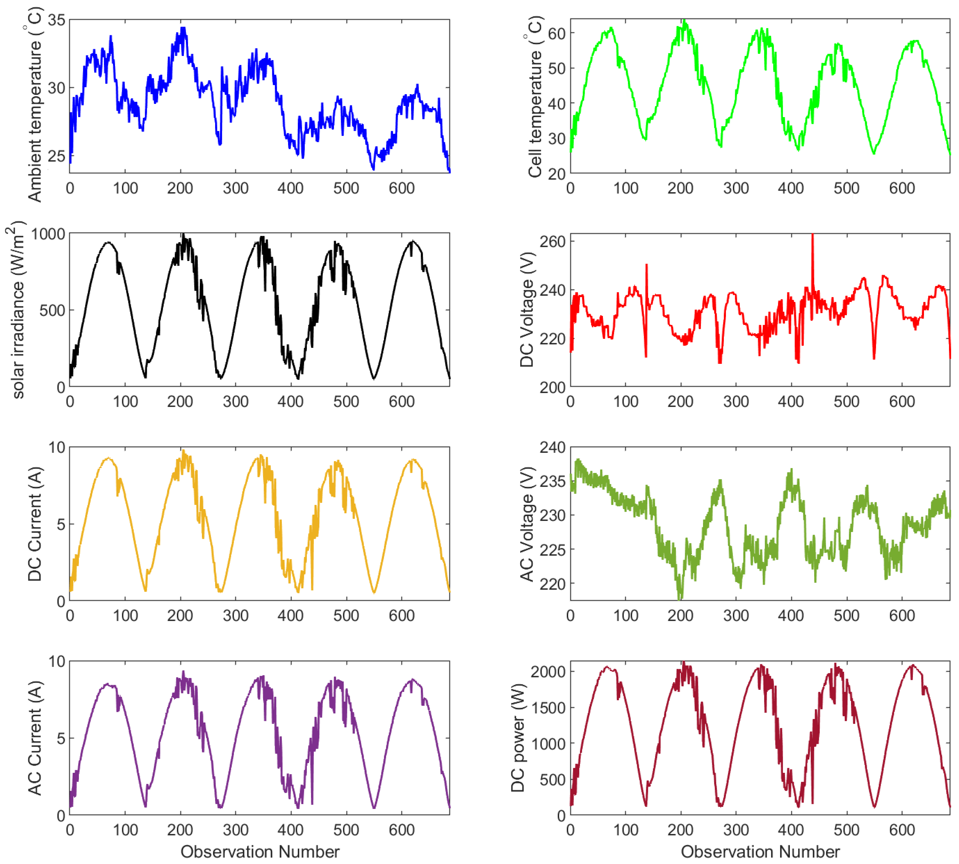
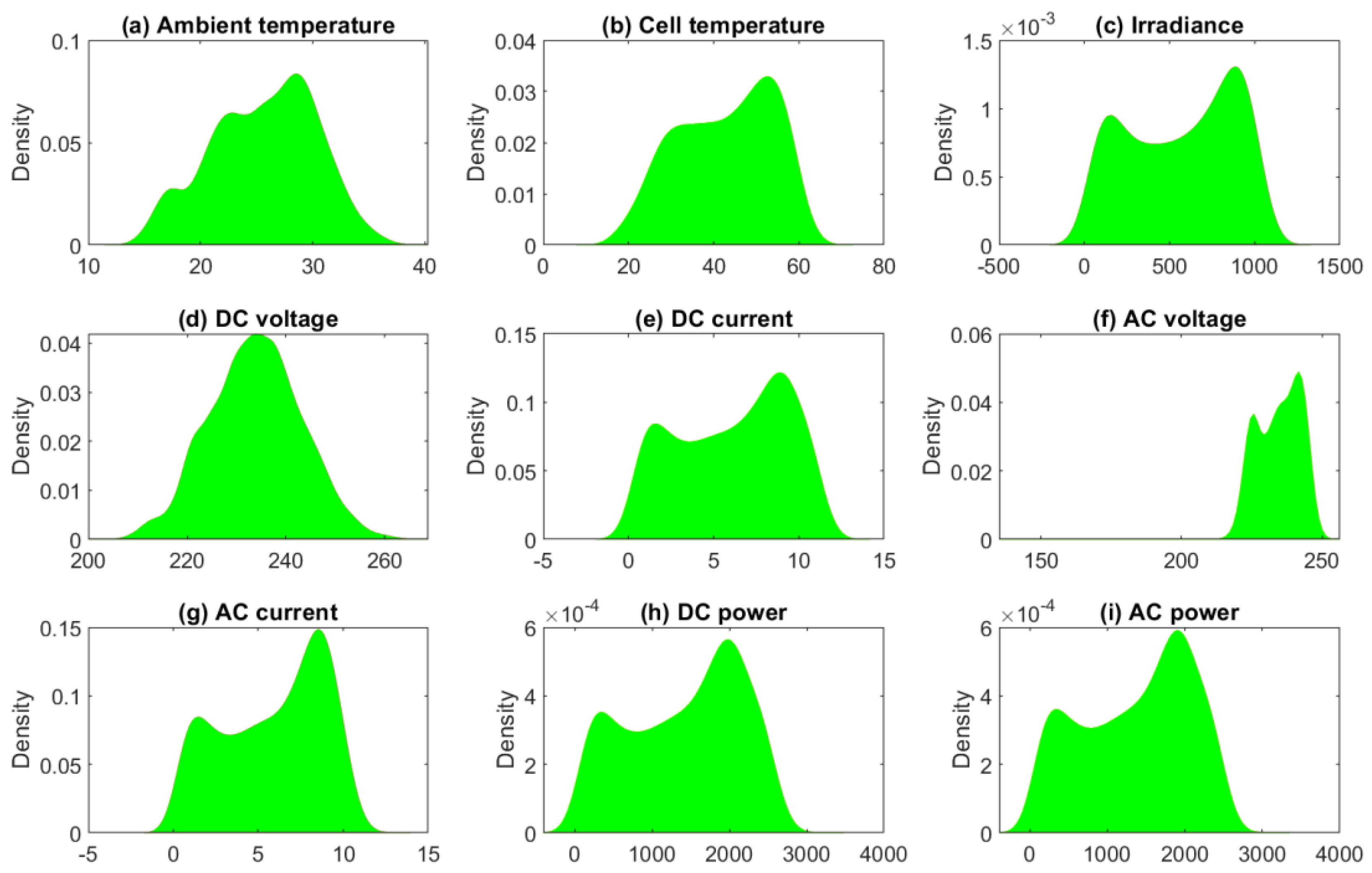
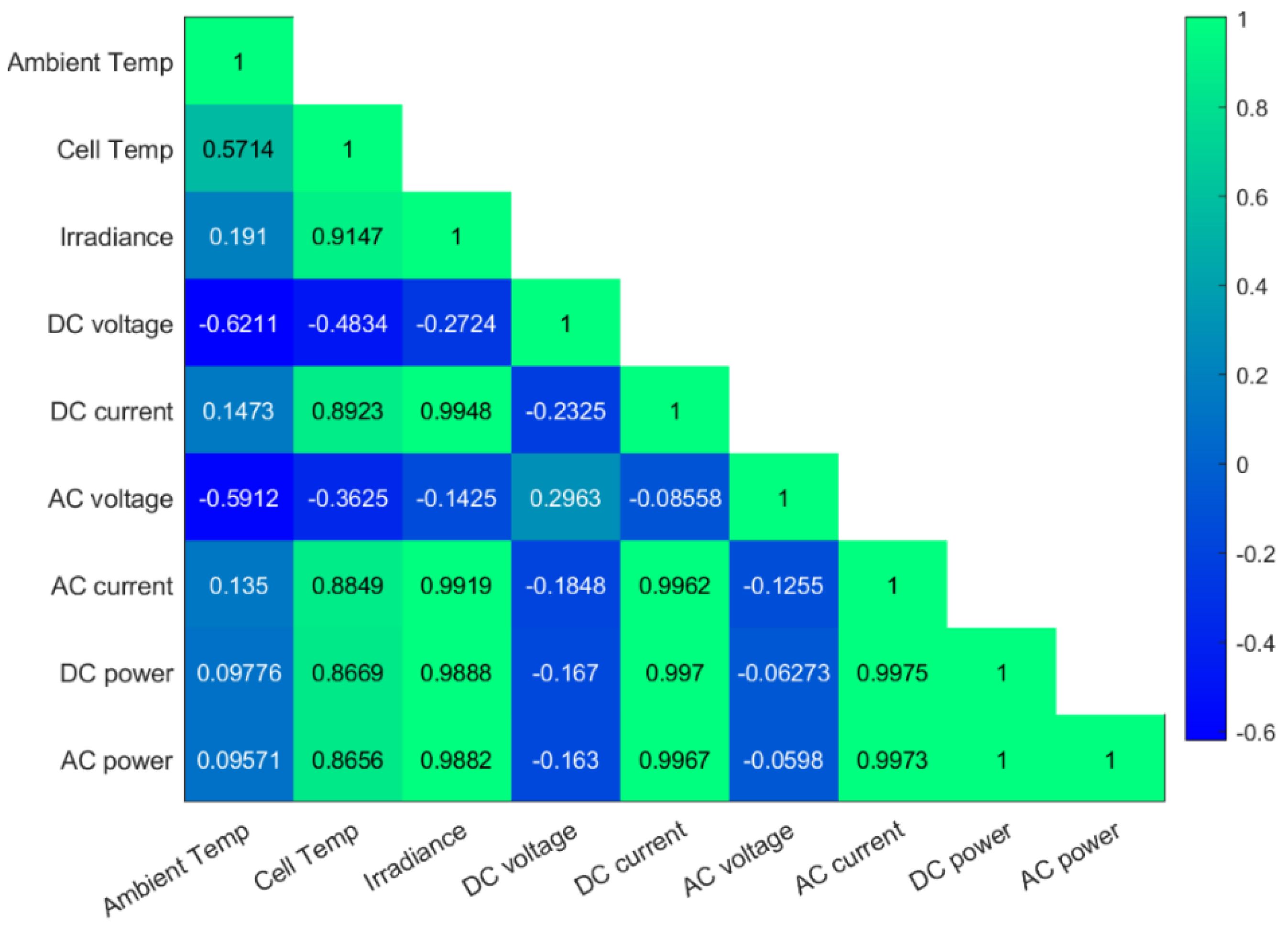
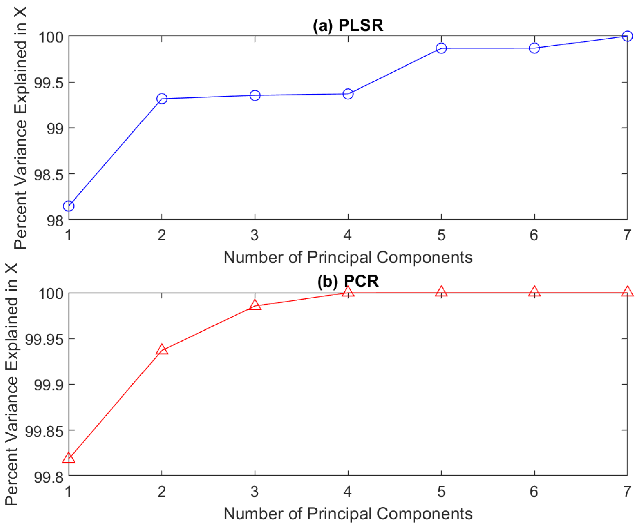
3.5. Dataset Analysis

The data used in this work has been gathered using the above-described CDER 9.54 kWp PV system (Figure 1). We consider here one month of measurement recorded with a cadence of 10 min during the normal operation of the monitored system. Precisely, the dataset is divided into training data that includes the free first week and used principally during the learning phase; and testing data (week four) which will be applied in the assessment of our proposed models. The provided measurements concern the following variables: solar irradiance, ambient temperature, cell temperature, DC power, DC current, DC voltage, AC power, AC current, and AC voltage. Figure 6 shows five days from the considered data.
Figure 7 depicts the estimated (PDF) of training data based on the KDE approach. We observe that the considered variables have non-Gaussian distribution. Thus, applying the conventional monitoring charts (e.g., TEWMA) is not appropriate as the assumption of normality is violated. Hence, using an appropriate model to capture the dynamic in this data and generate uncorrelated residuals is needed.
Here, the correlation between the nine variables is quantified using the Pearson correlation heatmap, as illustrated in Figure 8. We can conclude from Figure 8 that DC current, DC power, AC current, and AC power are highly correlated. Moreover, the cell temperature is strongly related to DC current, DC power, AC current, and AC power. Negative correlation between DC voltage and cell temperature. The AC voltage is totally uncorrelated with the rest of the variables. The irradiance, cell temperature, current DC, AC current, power DC, and power AC present a high correlation between them. Finally, a low correlation is reported between the DC voltage and the ambient cell temperature, the DC current, AC current, DC power, and AC power.
In PCR and PLS models, the number of selected PCs can strongly affect the quality of the constructed prediction models. We have applied the cumulative percentage variance (CPV) method to determine the suitable number of CPs. As depicted in Figure 9, the obtained results show that five and four CPs are needed to describe 99.87% of the variability in X for both PLS (Figure 9a) and 99.98 for PCR (Figure 9b) models, respectively.
Figure 10 presents the scatter plot of the measured and predicted DC power using PLS and PCR models based on testing data. Overall, results indicate that both models have allowed good prediction, and relatively PLS provided highest prediction quality.
Figure 11 shows the boxplots of residual errors of PLS and PCR models obtained with training data. As illustrated, best prediction results are obtained with PLS model.
In fact, the PLS model returned the smallest residual prediction errors, where most values were close to zero, resulting in the compacter box compared to PCR.

4. The LVR-TEWMA-Based Fault Detection in PV Systems

This section presents the key concept of the proposed fault detection approach for PV systems monitoring. In this work, at first, latent variable regression methods (i.e., PCR and PLS) are calibrated using normal operating data from the inspected PV system. Then, the calibrated models are employed to sense any anomalies in new data via the TEWMA statistical monitoring charts. The deviation (called residuals) between the measured data and the prediction from the constructed LVR models (i.e., PCR and PLS) delivers pertinent information and can be evaluated to uncover anomalies in the PV system. Reasonably, when the inspected PV system is operating customarily, the residuals fluctuate around zero because of noise measurements. On the other hand, if an atypical event or an anomaly occurs in the PV system, the residuals diverge from zero to reveal that the PV system requires attention. Figure 12 schematically recapitulates the proposed LVR-TEWMA anomaly detection framework.
Succinctly, the PLS residuals are expressed as follows:
R = Y Y ^
After that, we applied the TEWMA chart to evaluate the residuals for anomaly detection purposes. The LVR-TEWMA anomaly detection strategy can be mainly split into two phases. (1) During the model construction phase, we calibrate the LVR models and compute the TEWMA decision threshold based on normal operating data. (2) In the monitoring phase, we generate the residuals via the constructed LVR models and apply the already computed TEWMA threshold for monitoring new data. Here, we applied the KDE approach to determine the reference threshold. To do so, we estimate the PDF of the TEWMA measurements through KDE. Next, the detection threshold of the LVR-TEWMA approach is obtained as the (1 − α)-th quantile of the estimated PDF in respect of targeted false alarm probability α.
In summary, after building the LVR models and computing the TEWMA decision threshold, the new online data can be evaluated to sense potential anomalies. Specifically, the TEWMA charting statistic is compared with the detection threshold, H, to decide about the presence of an anomaly as follows:
δ = { N o   a n o m a l y         i f   T E W M A < H , A n o m a l y               i f   T E W M A > H .

5. Results

This section verifies the performance of the proposed LVR-TWEMA approaches in detecting several types of anomalies in PV systems that are recorded during real plants’ lifetime. Here, we focus our study on the DC side of PV systems, and we consider here specifically the following scenarios: String faults (SF), Inverter Disconnections (ID), Scenarios with Circuit Breaker Faults, Short-Circuit Faults (SCF), and Sensor Faults in Pyranometer (SFP). Different scenarios are carried out using real measurements gathered using the CDER 9.54 kWp PV system described in Section 2. The normal and faulty data were selected in the summer when most days are characterized by clear skies and medium ambient air temperature (which ranges from 20 to 35 °C). We employed five statistical metrics for the evaluation: true positive rate (TPR), false positive rate (FPR), accuracy, the area under curve (AUC), and EER (equal error rate) [62].

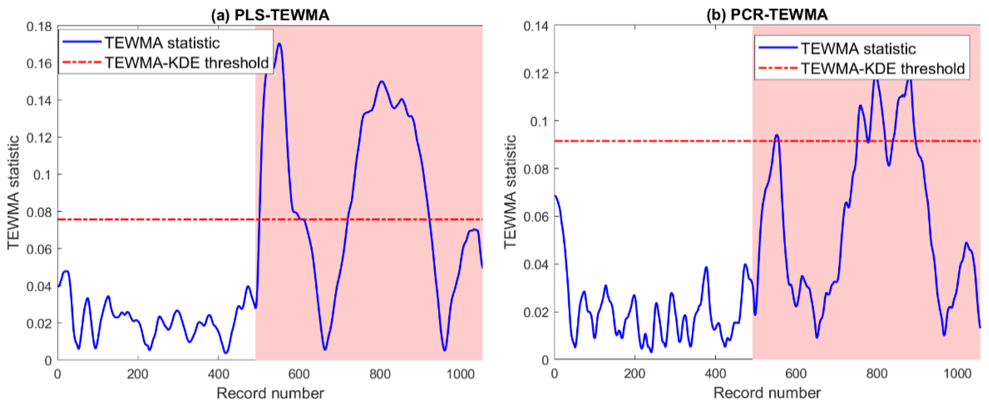
5.1. Scenarios with String Faults

The aim of this experiment is to assess the capacity of LVR-TWMA approaches to uncover the string’s fault (i.e., open circuits). Broadly speaking, Open circuits are generally related to the degradation of DC protection or detachment between PV modules in series. Here, we deactivate the circuit breaker to voluntarily create the desired open circuit faults. Figure 13 presents the corresponding detection results using the PLS- and PCR-based TEWMA methods. Both methods detect this fault with large magnitude. Table 3 quantitatively confirms the obtained results in terms of the five scores. Both methods reach a high detection rate, with no false alarms and an accuracy of 0.9942.

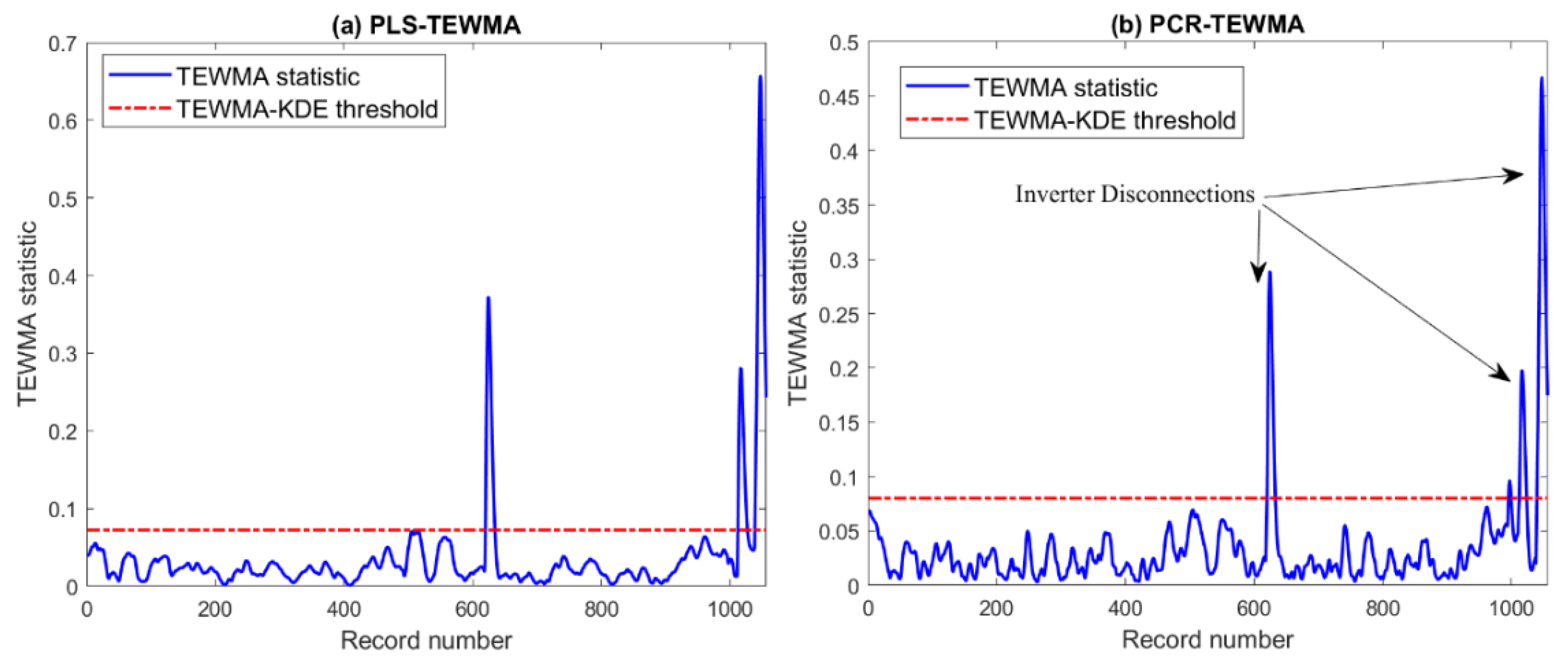
5.2. Scenarios with Inverter Disconnections

We now investigate the monitoring efficiency of the LVR-TEWMA methods in the presence of inverter disconnections in the inspected PV system. In this case, the PV system will still shut down till the inverter is reconnected. Here, we consider inverter disconnections resulted due to grid instability. More specifically, inverter disconnections refer to a situation where the voltage and frequency of the grid exceed the inverter operating limits. Inverter disconnections are short in time and have large amplitude. In this case study, we used real data with inverter disconnections to study the performance of the proposed monitoring techniques.
Figure 14 depicts the results of the PLS-TWEMA and PCR-TEWMA schemes. We observe that the two schemes successfully flagged the occurred inverter disconnections; these anomalies are with large amplitude. We also notice that these anomalies are within short periods, which can be very helpful in distinguishing them from other abnormal conditions, such as temporary shading and string faults. Table 4 summarizes the results of this comparison using the five statistical metrics. Results show that the PLS-TEWMA approach outperformed the PCR-TEWMA approach in detecting all occurred faults (i.e., TPR = 100%).

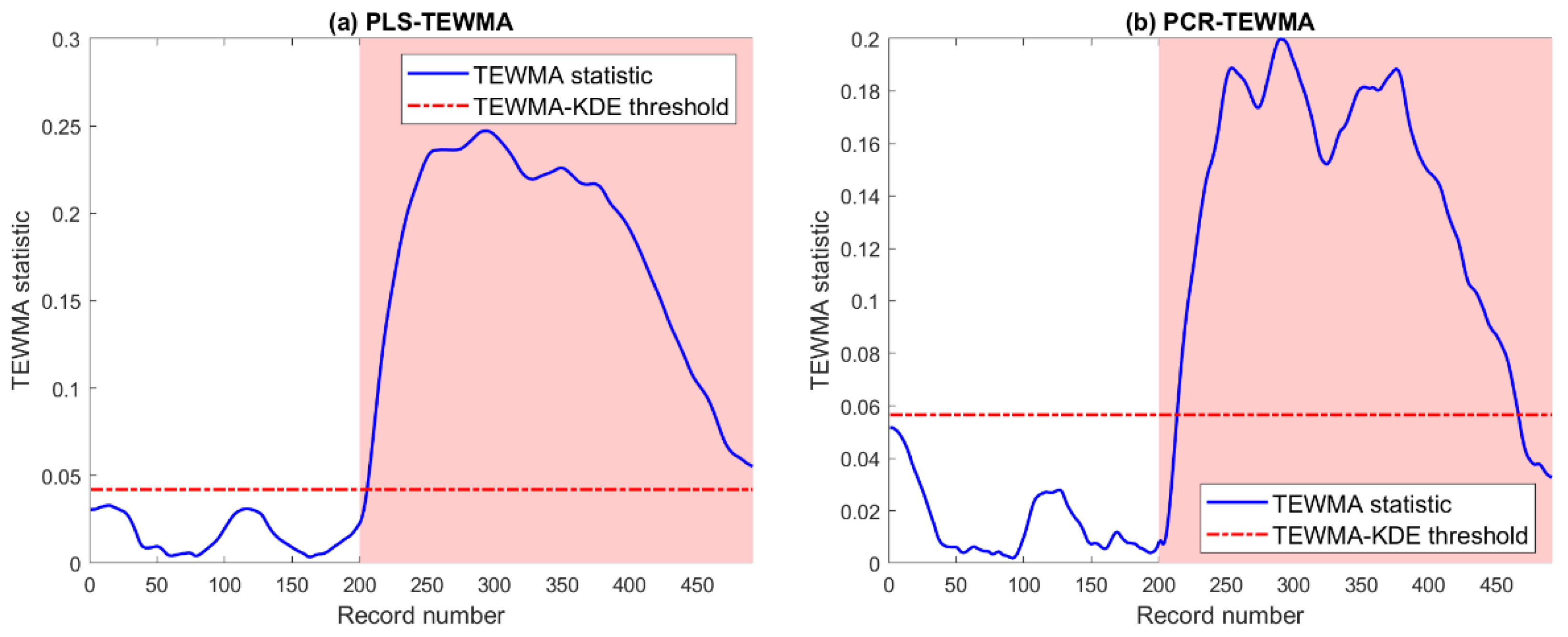
5.3. Scenario with Circuit Breaker Faults

Now, we assess the performances of the proposed methodologies under circuit breaker faults. These components are principally designed to protect PV systems and users from eventual shocks, short circuits, and potential overloads. Figure 15 and Table 5 illustrate the detection results of the PLS-TEWMA and PCR-TEWMA methods in the presence of RCCB faults. In overall, it is clear that both PLS and PCR maintain high performance with this type of fault. They reach a high detection rate with a TPR of around 0.98.

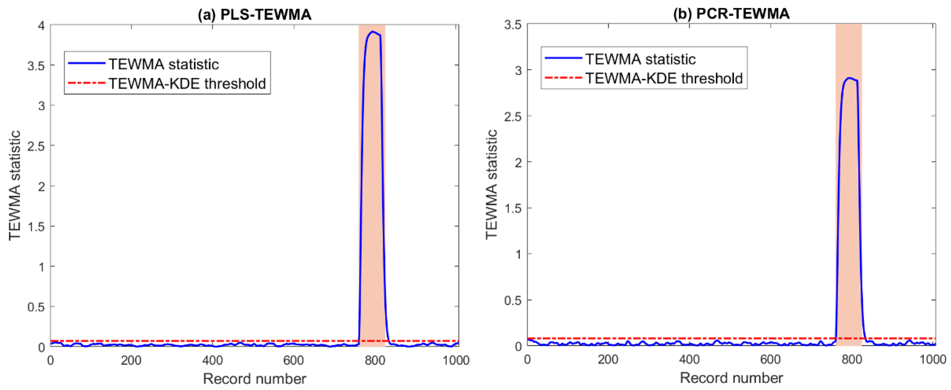
5.4. Short-Circuit Fault

In this scenario, the proposed methods are evaluated to detect short-circuit faults. Figure 16 displays the results of the two approaches when two PV modules are short-circuited. We can see that the two approaches can uncover this fault. Table 6 indicates that the PLS-TEWMA has the best performance, with a TPR of 0.8649. On the contrary, the PCR-TEWMA provides unsatisfactory results with high missed detection (TPR = 0.1351). This could be attributed to the prediction accuracy of the PLS model and the sensitivity of the TEWMA chart to the small changes.

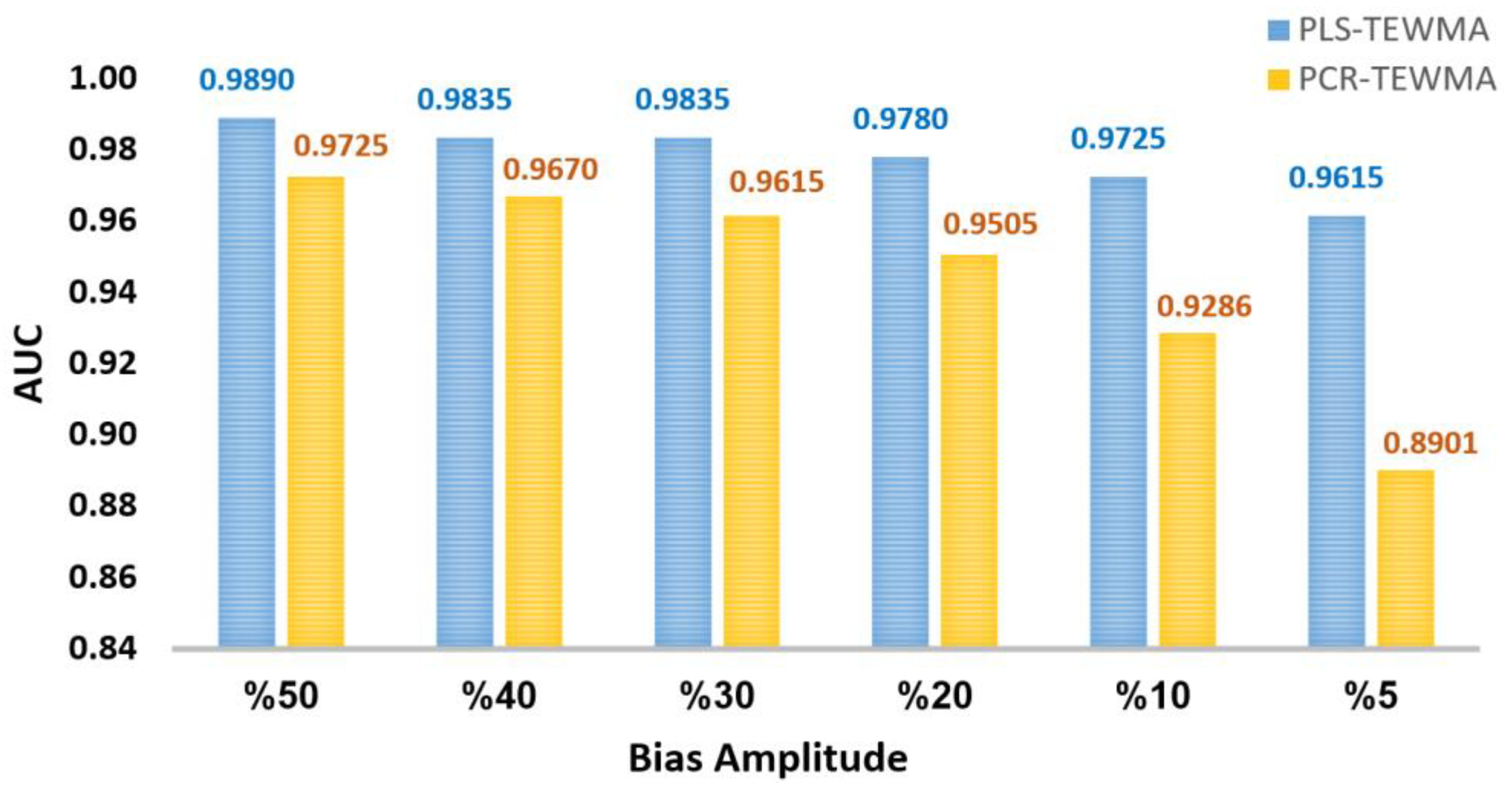
5.5. Sensor Bias Faults in the Pyranometer

We now consider sensor faults in pyranometers that could be due to degradation, aging, or other factors. Importantly, the pyranometer adapts the PV modules’ direction to optimally track the sun’s movements and be continuously highly exposed to sunlight. Consequently, faults affecting this precious component can prevent the PV system from being in the right orientation, which can significantly decrease the produced energy. Here, we simulate bias faults with different magnitudes to assess the sensitivity of the two proposed approaches. The simulated bias, b, begins at sample 200. We used the following model to simulate bias faults in the solar irradiance measurements.
y i = x i + b ,  
where y i and x i are the faulty and fault-free measurements, respectively. Here, as part of the total variation in solar irradiance measurements, we consider the following magnitudes: 5%, 10%, 20%, 30%, 40%, and 50%.
Detection results of the PLS-TEWMA and PCR-TEWMA charts in the case of bias faults (with 10%) in the pyranometer measurements are depicted in Figure 17. Visually, Figure 15 shows that both charts can recognize this bias fault. A comparison between the two charts under the presence of bias faults with different magnitudes is given in Table 7.
Detection results of the PLS-TEWMA and PCR-TEWMA charts in the case of bias faults (with 10%) in the pyranometer measurements are depicted in Figure 17. Visually, Figure 17 shows that both charts can recognize this bias fault. A comparison between the two charts under the presence of bias faults with different magnitudes is given in Table 8. Results in Table 8 confirm the superiority of the PLS-TEWMA scheme compared to the PCR-TEWMA, particularly for faults with small levels. For instance, for bias faults with 5%, the PLS-TEMWA scheme detects this sensor fault with a TPR of 0.9231, while the PCR-TEWMA scheme obtains a TPR of 0.7802.
Figure 18 depicts the AUC values of the two charts for the considered faults. The main conclusion from Figure 18 is that when the amplitude of the occurred fault is small, the PLS-TEWMA scheme is better than the PCR-TEWMA scheme. On the other hand, for a large fault, the two schemes are comparable.
For comparison purposes, we applied PLS- and PCR-based double EWMA (DEWMA) charts to detect bias sensors fault in the pyranometer (Table 8). Here, we also used the KDE approach to estimate the decision thresholds for the two charts, which enables more detection flexibility. From Table 8, we observe that for abnormal changes with large magnitudes, the two approaches (i.e., PLS-DEWMA and PCR-DEWMA) achieved relatively comparable performance, while for small changes, the PLS-DEWM chart outperformed the PCR-DEMWA approach.
From Table 7 and Table 8, we observe that the PLS- and PCR-based TEWMA charts showed improved detection ability compared to the PLS- and PCR-based DEWMA chart, particularly for small faults. At the same time, they are relatively comparable for moderate and large faults. Overall, the proposed PLS-TEWMA approach is more effective in detecting small faults compared to the other charts. This is mainly due to the capacity of the TEWMA chart to sense small changes in data. However, the results revealed that the PLS-TEWMA approach can sense small changes but with some missed detection (TPR = 0.9231) (Table 7). This could be attributed to the used PLS model, which is a linear model, that is not suited to capture process nonlinearity. Thus, we recommend adopting nonlinear models, such as nonlinear PLS, to enhance the detection capability of the proposed approach.

6. Conclusions

This study is within a data-driven anomaly detection framework for PV systems monitoring. An efficient strategy combining latent variable regression methods (i.e., PCR and PLS) with the TEWMA monitoring chart has been developed to detect anomalies in the DC sides of PV systems. Specifically, LVR methods have been built using training data and then used to generate residuals, which are used as anomaly indicators. Here, the TEWMA chart is applied to residuals for fault detection. The decision threshold in the TEWMA chart is determined using a KDE-based approach to allow more flexibility and improve detection accuracy. Several real anomalies and simulated sensor faults have been considered to study the performance of the proposed approaches. Results revealed that the PLS-TEWMA chart provided superior detection performance compared to that of the PCR-TEWMA chart and PLS- and PCR-based DEWMA charts, particularly for small faults.
In future work, we plan to improve the proposed technique by incorporating machine learning-based classification methods to discriminate between the detected anomalies. Another direction of improvement consists of amalgamating the benefit of deep-learning models [45,63] and the detection capacity of the TEWMA to sense small changes. In addition, it will be interesting to investigate the detection capability of this approach in uncovering other types of sensor anomalies, such as sensor degradation anomalies, sensor-freezing anomalies, and multiple sensor anomalies that affect different sensors (e.g., pyranometers and thermocouples) simultaneously. Data from PV plants is tainted with noise, which can degrade the detection performance by increasing the number of false alarms rate in the case of a low signal-to-noise ratio. We also plan in future work to construct a robust detection approach that combines wavelet multiscale presentation with the TEWMA chart.

Author Contributions

B.B.: Conceptualization, formal analysis, investigation, methodology, software, writing—original draft, and writing—review and editing. F.H.: Conceptualization, formal analysis, investigation, methodology, software, supervision, writing—original draft, and writing—review and editing. B.T.: Formal analysis, software, funding acquisition, writing—original draft, and writing—review and editing. Y.S.: Investigation, conceptualization, formal analysis, methodology, writing—review and editing, and supervision. A.H.A.: project administration, funding acquisition, and writing—review and editing. All authors have read and agreed to the published version of the manuscript.

Funding

This work was supported by funding from the King Abdullah University of Science and Technology (KAUST), Office of Sponsored Research (OSR), under Award No: OSR-2019-CRG7-3800, and from the Centre de Développement des Energies Renouvelables (CDER), Direction Générale de la Recherche Scientifique et du Développement Technologique (DGRSDT).

Institutional Review Board Statement

Not applicable.

Informed Consent Statement

Not applicable.

Data Availability Statement

Not applicable.

Conflicts of Interest

The authors declare no conflict of interest.

References

  1. Ahmed, W.; Sheikh, J.A.; Farjana, S.H.; Mahmud, M.A.P. Defects Impact on PV System GHG Mitigation Potential and Climate Change. Sustainability 2021, 13, 7793. [Google Scholar] [CrossRef]
  2. IEA PVPS. Trends in Photovoltaic Applications. 2021. Available online: https://tecsol.blogs.com/files/iea-pvps-trends-report-2021-1.pdf (accessed on 23 October 2022).
  3. Garoudja, E.; Harrou, F.; Sun, Y.; Kara, K.; Chouder, A.; Silvestre, S. Statistical fault detection in photovoltaic systems. Sol. Energy 2017, 150, 485–499. [Google Scholar] [CrossRef]
  4. Alam, M.K.; Khan, F.; Johnson, J.; Flicker, J. A comprehensive review of catastrophic faults in PV arrays: Types, detection, and mitigation techniques. IEEE J. Photovolt. 2015, 5, 982–997. [Google Scholar] [CrossRef]
  5. Hare, J.; Shi, X.; Gupta, S.; Bazzi, A. Fault diagnostics in smart micro-grids: A survey. Renew. Sustain. Energy Rev. 2016, 60, 1114–1124. [Google Scholar] [CrossRef]
  6. Ye, J.; Giani, A.; Elasser, A.; Mazumder, S.K.; Farnell, C.; Mantooth, H.A.; Kim, T.; Liu, J.; Chen, B.; Seo, G.S.; et al. A Review of Cyber–Physical Security for Photovoltaic Systems. IEEE J. Emerg. Sel. Top. Power Electron. 2021, 10, 4879–4901. [Google Scholar] [CrossRef]
  7. Wang, W.; Harrou, F.; Bouyeddou, B.; Senouci, S.M.; Sun, Y. A stacked deep learning approach to cyber-attacks detection in industrial systems: Application to power system and gas pipeline systems. Clust. Comput. 2022, 25, 561–578. [Google Scholar] [CrossRef]
  8. Wang, W.; Harrou, F.; Bouyeddou, B.; Senouci, S.M.; Sun, Y. Cyber-attacks detection in industrial systems using artificial intelligence-driven methods. Int. J. Crit. Infrastruct. Prot. 2022, 38, 100542. [Google Scholar] [CrossRef]
  9. Le, M.; Nguyen, D.K.; Dao, V.D.; Vu, N.H.; Vu, H.H.T. Remote anomaly detection and classification of solar photovoltaic modules based on deep neural network. Sustain. Energy Technol. Assess. 2021, 48, 101545. [Google Scholar] [CrossRef]
  10. Janarthanan, R.; Maheshwari, R.U.; Shukla, P.K.; Shukla, P.K.; Mirjalili, S.; Kumar, M. Intelligent detection of the PV faults based on artificial neural network and type 2 fuzzy systems. Energies 2021, 14, 6584. [Google Scholar] [CrossRef]
  11. Harrou, F.; Saidi, A.; Sun, Y.; Khadraoui, S. Monitoring of photovoltaic systems using improved kernel-based learning schemes. IEEE J. Photovolt. 2021, 11, 806–818. [Google Scholar] [CrossRef]
  12. Mellit, A.; Tina, G.M.; Kalogirou, S.A. Fault detection and diagnosis methods for photovoltaic systems: A review. Renew. Sustain. Energy Rev. 2018, 91, 1–17. [Google Scholar] [CrossRef]
  13. Madeti, S.R.; Singh, S.N. Modeling of PV system based on experimental data for fault detection using kNN method. Sol. Energy 2018, 173, 139–151. [Google Scholar] [CrossRef]
  14. Badr, M.M.; Hamad, M.S.; Abdel-Khalik, A.S.; Hamdy, R.A.; Ahmed, S.; Hamdan, E. Fault Identification of Photovoltaic Array Based on Machine Learning Classifiers. IEEE Access 2021, 9, 159113–159132. [Google Scholar] [CrossRef]
  15. Benkercha, R.; Moulahoum, S. Fault detection and diagnosis based on C4. 5 decision tree algorithm for grid connected PV system. Sol. Energy 2018, 173, 610–634. [Google Scholar] [CrossRef]
  16. Harrou, F.; Taghezouit, B.; Sun, Y. Robust and flexible strategy for fault detection in grid-connected photovoltaic systems. Energy Convers. Manag. 2019, 180, 1153–1166. [Google Scholar] [CrossRef]
  17. Harrou, F.; Dairi, A.; Taghezouit, B.; Sun, Y. An unsupervised monitoring procedure for detecting anomalies in photovoltaic systems using a one-class Support Vector Machine. Sol. Energy 2019, 179, 48–58. [Google Scholar] [CrossRef]
  18. Harrou, F.; Sun, Y.; Taghezouit, B.; Saidi, A.; Hamlati, M.E. Reliable fault detection and diagnosis of photovoltaic systems based on statistical monitoring approaches. Renew. Energy 2018, 116, 22–37. [Google Scholar] [CrossRef] [Green Version]
  19. Huang, C.M.; Chen, S.J.; Yang, S.P. A Parameter Estimation Method for a Photovoltaic Power Generation System Based on a Two-Diode Model. Energies 2022, 15, 1460. [Google Scholar] [CrossRef]
  20. Kang, B.K.; Kim, S.T.; Bae, S.H.; Park, J.W. Diagnosis of output power lowering in a PV array by using the Kalman-filter algorithm. IEEE Trans. Energy Convers. 2012, 27, 885–894. [Google Scholar] [CrossRef]
  21. Skomedal, Å.F.; Øgaard, M.B.; Haug, H.; Marstein, E.S. Robust and fast detection of small power losses in large-scale PV systems. IEEE J. Photovolt. 2021, 11, 819–826. [Google Scholar] [CrossRef]
  22. Spataru, S.; Sera, D.; Kerekes, T.; Teodorescu, R. Diagnostic method for photovoltaic systems based on light I–V measurements. Sol. Energy 2015, 119, 29–44. [Google Scholar] [CrossRef]
  23. Chouder, A.; Silvestre, S. Automatic supervision and fault detection of PV systems based on power losses analysis. Energy Convers. Manag. 2010, 51, 1929–1937. [Google Scholar] [CrossRef]
  24. Hou, Z.S.; Wang, Z. From model-based control to data-driven control: Survey, classification and perspective. Inf. Sci. 2013, 235, 3–35. [Google Scholar] [CrossRef]
  25. Taghezouit, B.; Harrou, F.; Sun, Y.; Arab, A.H.; Larbes, C. Multivariate statistical monitoring of photovoltaic plant operation. Energy Convers. Manag. 2020, 205, 112317. [Google Scholar] [CrossRef]
  26. Fadhel, S.; Delpha, C.; Diallo, D.; Bahri, I.; Migan, A.; Trabelsi, M.; Mimouni, M.F. PV shading fault detection and classification based on IV curve using principal component analysis: Application to isolated PV system. Sol. Energy 2019, 179, 1–10. [Google Scholar] [CrossRef] [Green Version]
  27. Amaral, T.G.; Pires, V.F.; Pires, A.J. Fault detection in PV tracking systems using an image processing algorithm based on PCA. Energies 2021, 14, 7278. [Google Scholar] [CrossRef]
  28. Deceglie, M.G.; Micheli, L.; Muller, M. Quantifying soiling loss directly from PV yield. IEEE J. Photovolt. 2018, 8, 547–551. [Google Scholar] [CrossRef]
  29. Kiliç, H.; Gumus, B.; Khaki, B.; Yilmaz, M.; Palensky, P.; Authority, P. A Robust Data-Driven Approach for Fault Detection in Photovoltaic Arrays. In Proceedings of the 10th IEEE PES Innovative Smart Grid Technologies Europe, ISGT-Europe 2020, Virtual, 26–28 October 2020. [Google Scholar]
  30. Xiong, Q.; Liu, X.; Feng, X.; Gattozzi, A.L.; Shi, Y.; Zhu, L.; Ji, S.; Hebner, R.E. Arc fault detection and localization in photovoltaic systems using feature distribution maps of parallel capacitor currents. IEEE J. Photovolt. 2018, 8, 1090–1097. [Google Scholar] [CrossRef]
  31. Kumar, B.P.; Ilango, G.S.; Reddy, M.J.B.; Chilakapati, N. Online fault detection and diagnosis in photovoltaic systems using wavelet packets. IEEE J. Photovolt. 2017, 8, 257–265. [Google Scholar] [CrossRef]
  32. Edun, A.S.; Kingston, S.; LaFlamme, C.; Benoit, E.; Scarpulla, M.A.; Furse, C.M.; Harley, J.B. Detection and localization of disconnections in a large-scale string of photovoltaics using SSTDR. IEEE J. Photovolt. 2021, 11, 1097–1104. [Google Scholar] [CrossRef]
  33. Wang, M.H.; Lin, Z.H.; Lu, S.D. A Fault Detection Method Based on CNN and Symmetrized Dot Pattern for PV Modules. Energies 2022, 15, 6449. [Google Scholar] [CrossRef]
  34. Cui, F.; Tu, Y.; Gao, W. A Photovoltaic System Fault Identification Method Based on Improved Deep Residual Shrinkage Networks. Energies 2022, 15, 3961. [Google Scholar] [CrossRef]
  35. Harrou, F.; Taghezouit, B.; Sun, Y. Improved kNN-based monitoring schemes for detecting faults in PV systems. IEEE J. Photovolt. 2019, 9, 811–821. [Google Scholar] [CrossRef]
  36. Harrou, F.; Taghezouit, B.; Khadraoui, S.; Dairi, A.; Sun, Y.; Hadj Arab, A. Ensemble Learning Techniques-Based Monitoring Charts for Fault Detection in Photovoltaic Systems. Energies 2022, 15, 6716. [Google Scholar] [CrossRef]
  37. Karatepe, E.; Hiyama, T. Controlling of artificial neural network for fault diagnosis of photovoltaic array. In Proceedings of the 2011 16th International Conference on Intelligent System Applications to Power Systems, Hersonissos, Greece, 25–28 September 2011; pp. 1–6. [Google Scholar]
  38. Chen, S.Q.; Yang, G.J.; Gao, W.; Guo, M.F. Photovoltaic fault diagnosis via semisupervised ladder network with string voltage and current measures. IEEE J. Photovolt. 2020, 11, 219–231. [Google Scholar] [CrossRef]
  39. Gaggero, G.B.; Rossi, M.; Girdinio, P.; Marchese, M. Detecting System Fault/Cyberattack within a Photovoltaic System Connected to the Grid: A Neural Network-Based Solution. J. Sens. Actuator Netw. 2020, 9, 20. [Google Scholar] [CrossRef] [Green Version]
  40. Parvez, I.; Aghili, M.; Sarwat, A.I.; Rahman, S.; Alam, F. Online power quality disturbance detection by support vector machine in smart meter. J. Mod. Power Syst. Clean Energy 2019, 7, 1328–1339. [Google Scholar] [CrossRef] [Green Version]
  41. Madakyaru, M.; Harrou, F.; Sun, Y. Monitoring distillation column systems using improved nonlinear partial least squares-based strategies. IEEE Sens. J. 2019, 19, 11697–11705. [Google Scholar] [CrossRef] [Green Version]
  42. Kourti, T.; MacGregor, J.F. Process analysis, monitoring and diagnosis, using multivariate projection methods. Chemom. Intell. Lab. Syst. 1995, 28, 3–21. [Google Scholar] [CrossRef]
  43. Geladi, P.; Kowalski, B.R. Partial least-squares regression: A tutorial. Anal. Chim. Acta 1986, 185, 1–17. [Google Scholar] [CrossRef]
  44. Harrou, F.; Sun, Y.; Madakyaru, M. Kullback-leibler distance-based enhanced detection of incipient anomalies. J. Loss Prev. Process Ind. 2016, 44, 73–87. [Google Scholar] [CrossRef]
  45. Harrou, F.; Sun, Y.; Hering, A.S.; Madakyaru, M.; Dairi, A. Linear Latent Variable Regression (LVR)-Based Process Monitoring; Elsevier BV: Amsterdam, The Netherlands, 2021. [Google Scholar]
  46. Li, B.; Morris, J.; Martin, E.B. Model selection for partial least squares regression. Chemom. Intell. Lab. Syst. 2002, 64, 79–89. [Google Scholar] [CrossRef]
  47. MacGregor, J.F.; Kourti, T. Statistical process control of multivariate processes. Control Eng. Pract. 1995, 3, 403–414. [Google Scholar] [CrossRef]
  48. Madakyaru, M.; Harrou, F.; Sun, Y. Improved data-based fault detection strategy and application to distillation columns. Process Saf. Environ. Prot. 2017, 107, 22–34. [Google Scholar] [CrossRef] [Green Version]
  49. Wang, X.; Kruger, U.; Lennox, B. Recursive partial least squares algorithms for monitoring complex industrial processes. Control. Eng. Pract. 2003, 11, 613–632. [Google Scholar] [CrossRef]
  50. Ahn, S.J.; Lee, C.J.; Jung, Y.; Han, C.; Yoon, E.S.; Lee, G. Fault diagnosis of the multi-stage flash desalination process based on signed digraph and dynamic partial least square. Desalination 2008, 228, 68–83. [Google Scholar] [CrossRef]
  51. Bouyeddou, B.; Harrou, F.; Saidi, A.; Sun, Y. An Effective Wind Power Prediction using Latent Regression Models. In Proceedings of the 2021 International Conference on ICT for Smart Society (ICISS), Bandung, Indonesia, 2–4 August 2021; pp. 1–6. [Google Scholar]
  52. Frank, L.E.; Friedman, J.H. A statistical view of some chemometrics regression tools. Technometrics 1993, 35, 109–135. [Google Scholar] [CrossRef]
  53. Harrou, F.; Nounou, M.N.; Nounou, H.N. Detecting abnormal ozone levels using PCA-based GLR hypothesis testing. In Proceedings of the 2013 IEEE Symposium on Computational Intelligence and Data Mining (CIDM), Singapore, 16–19 April 2013; pp. 95–102. [Google Scholar]
  54. Alevizakos, V.; Chatterjee, K.; Koukouvinos, C. The triple exponentially weighted moving average control chart. Qual. Technol. Quant. Manag. 2021, 18, 326–354. [Google Scholar] [CrossRef]
  55. Alevizakos, V.; Chatterjee, K.; Koukouvinos, C. A nonparametric triple exponentially weighted moving average sign control chart. Qual. Reliab. Eng. Int. 2021, 37, 1504–1523. [Google Scholar] [CrossRef]
  56. Mahmoud, M.A.; Woodall, W.H. An evaluation of the double exponentially weighted moving average control chart. Commun. Stat.—Simul. Comput. 2010, 39, 933–949. [Google Scholar] [CrossRef]
  57. Zhang, L.; Chen, G. An extended EWMA mean chart. Qual. Technol. Quant. Manag. 2005, 2, 39–52. [Google Scholar] [CrossRef]
  58. Zhang, L.; Bebbington, M.S.; Govindaraju, K.; Lai, C.D. Composite EWMA control charts. Commun. Stat.-Simul. Comput. 2004, 33, 1133–1158. [Google Scholar] [CrossRef]
  59. Martin, E.; Morris, A. Non-parametric confidence bounds for process performance monitoring charts. J. Proc. Control 1996, 6, 349–358. [Google Scholar] [CrossRef]
  60. Chen, Y.C. A tutorial on kernel density estimation and recent advances. Biostat. Epidemiol. 2017, 1, 161–187. [Google Scholar] [CrossRef]
  61. Mugdadi, A.R.; Ahmad, I.A. A bandwidth selection for kernel density estimation of functions of random variables. Comput. Stat. Data Anal. 2004, 47, 49–62. [Google Scholar] [CrossRef]
  62. Harrou, F.; Khaldi, B.; Sun, Y.; Cherif, F. An efficient statistical strategy to monitor a robot swarm. IEEE Sens. J. 2019, 20, 2214–2223. [Google Scholar] [CrossRef] [Green Version]
  63. Dairi, A.; Harrou, F.; Sun, Y.; Khadraoui, S. Short-term forecasting of photovoltaic solar power production using variational auto-encoder driven deep learning approach. Appl. Sci. 2020, 10, 8400. [Google Scholar] [CrossRef]
Figure 1. Picture of the PV Array of the GCPV system on the rooftop at CDER.
Energies 15 07978 g001
Figure 2. Illustrative diagram of the used grid-connected PV system.
Energies 15 07978 g002
Figure 3. Synoptic diagram of the PV monitoring system.
Energies 15 07978 g003
Figure 4. General design of PLS model.
Energies 15 07978 g004
Figure 5. General representation of PCR model.
Energies 15 07978 g005
Figure 6. Five days of the studied PV data.
Energies 15 07978 g006
Figure 7. Distribution of the considered variables.
Energies 15 07978 g007
Figure 8. Correlation matrix of training PV data.
Energies 15 07978 g008
Figure 9. Correlation matrix of training data.
Energies 15 07978 g009
Figure 10. Scatter plot of the measured and predicted DC power using PLS and PCR models.
Energies 15 07978 g010
Figure 11. Box plot of residual errors of PLS and PCR models.
Energies 15 07978 g011
Figure 12. General fault detection procedure in PV system using LVR-based KDE triple exponentially smoothing driven monitoring schemes.
Energies 15 07978 g012
Figure 13. Detection results of (a) PLS and (b) PCR-based TEWMA charts in the presence of string fault.
Energies 15 07978 g013
Figure 14. Detection results of (a) PLS- and (b) PCR-based TEWMA charts in the presence of inverter disconnections.
Energies 15 07978 g014
Figure 15. Detection results of (a) PLS- and (b) PCR-based TEWMA charts in the presence of RCCB faults.
Energies 15 07978 g015
Figure 16. Detection results of (a) PLS- and (b) PCR-based TEWMA charts in the presence of two short-circuited modules.
Energies 15 07978 g016
Figure 17. Detection results of (a) PLS- and (b) PCR-based TEWMA charts in the presence of sensor bias fault in the pyranometer measurements (a bias of 10% of the total variation in solar irradiance measurements).
Energies 15 07978 g017
Figure 18. AUC values by PLS- and PCR-based TEWMA charts for different bias magnitudes in the pyranometer.
Energies 15 07978 g018
Table 1. Electrical Characteristic of PV Module and PV sub-array Isofoton I106-12.
ParametersISC (A)VOC (V)IMPP (A)VMPP (V)PM (W)
PV Module6.5421.66.117.4106
PV Sub-Array13.0832412.22613180
Table 2. Electrical Characteristic of PV Inverter Fronius IG 30 under nominal conditions.
ParametersNominal AC
Power (W)
DC Voltage
Range (V)
Inverter
Efficiency (%)
AC Voltage
Range (V)
Frequency
Range (Hz)
Value2500150–40092.7–94.3195–25349.8–50.2
Table 3. Results of PLS-based and PCR-based TEWMA charts under string fault.
MethodTPRFPRAccuracyAUCEER
PLS-TEWMA0.9800.99420.990.0034
PCR-TEWMA0.9800.99420.990.0034
Table 4. Results of PLS- and PCR-based TEWMA charts under inverter disconnections.
MethodTPRFPRAccuracyAUCEER
PLS-TEWMA10.04180.95830.97910.0417
PCR-TEWMA0.750.03990.95930.85500.0407
Table 5. Results of PLS- and PCR-based TEWMA charts under RCCB faults.
MethodTPRFPRAccuracyAUCEER
PLS-TEWMA0.98150.02200.97820.97970.0218
PCR-TEWMA0.98150.02100.97910.98020.0209
Table 6. Results of PLS- and PCR-based TEWMA charts under two modules short-circuited.
MethodTPRFPRAccuracyAUCEER
PLS-TEWMA0.864900.98230.93240.0095
PCR-TEWMA0.135100.88670.56760.0606
Table 7. Results of PLS- and PCR-based TEWMA charts under bias sensors fault in pyranometer.
Bias
Sensor (B)
TEWMA
Method
TPRFPRAccuracyAUCEER
50%PLS0.978000.99310.98900.0041
PCR0.945100.98280.97250.0102
40%PLS0.967000.98970.98350.0061
PCR0.934100.97940.96700.0122
30%PLS0.967000.98970.98350.0061
PCR0.923100.97590.96150.0143
20%PLS0.956000.98630.97800.0081
PCR0.901100.96910.95050.0183
10%PLS0.945100.98280.97250.0102
PCR0.857100.95530.92860.0265
5%PLS0.923100.97590.96150.0143
PCR0.780200.93130.89010.0407
Table 8. Results of PLS- and PCR-based DEWMA charts under bias sensors fault in pyranometer.
Bias
Sensor (B)
DEWMA
Method
TPRFPRAccuracyAUCEER
50%PLS0.962200.97760.98110.0224
PCR0.955300.97350.97770.0265
40%PLS0.958800.97560.97940.0244
PCR0.931300.95930.96560.0407
30%PLS0.931300.95930.96560.0407
PCR0.903800.94300.95190.0570
20%PLS0.900300.94090.95020.0591
PCR0.872900.92460.93640.0754
10%PLS0.738800.84520.86940.1548
PCR0.745700.84930.87290.1507
5%PLS0.721600.83500.86080.1650
PCR0.697600.82080.84880.1792
Publisher’s Note: MDPI stays neutral with regard to jurisdictional claims in published maps and institutional affiliations.

