Intelligent Monitoring of Photovoltaic Systems via Simplicial Empirical Models and Performance Loss Rate Evaluation under LabVIEW: A Case Study

Abstract

The capacity of photovoltaic solar power installations has been boosted last years by reaching a new record with 175 GWdc of newly installed solar power in 2021. To guarantee reliable performances of photovoltaic (PV) plants and maintain target requirements, faults have to be reliably detected and diagnosed. A method for an effective and reliable fault diagnosis of PV plants based on the behavioral model and performance analysis under the LabVIEW environment is presented in this paper. Specifically, the first phase of this study consists of the behavioral modeling of the PV array and the inverter in order to estimate the electricity production and analyze the performance of the 9.54 kWp Grid Connected PV System (GCPVS). Here, the results obtained from the empirical models were validated and calibrated by experimental data. Furthermore, a user interface for modeling and analyzing the performance of a PV system under LabVIEW has been designed. The second phase of this work is dedicated to the design of a simple and efficient diagnostic tool in order to detect and recognize faults occurring in the PV systems. Essentially, the residuals obtained using the parametric models are analyzed via the performance loss rates (PLR) of four electrical indicators (i.e., DC voltage, DC current, DC power, and AC power). To evaluate the proposed method, numerous environmental anomalies and electrical faults affecting the GCPVS were taken into account. Results demonstrated the satisfactory prediction performance of the considered empirical models to predict the considered variables, including DC current, DC power, and AC power with an $R^2$ of 0.99. Moreover, the obtained results show that the detection and recognition of faults were successfully achieved.

1. Introduction

Renewable energy has become most attractive than before due to the clean and high-efficiency energy produced from renewable energy sources. Despite the economic slowdown caused by the COVID-19 pandemic, global renewable energy capacity has experienced rapid growth, adding more than 314 GW in 2021, which represents a growth of 17%, to reach 3146 GW of total installed capacity [1,2]. The solar photovoltaic (PV) market in recent years has seen strong expansion with at least 175 Gigawatts in direct current (GWdc) added in 2021, reaching a total installed capacity of 942 GWdc [3]. This growth is due to technology innovations and competitiveness in the solar PV market, electricity demand, low maintenance costs, and rapid return on investment [4]. Since the share of solar PV power is sharply increasing, safety and reliability during electricity production are becoming indispensable. For this purpose, national grid operators around the world require guaranteed availability and a high level of predictability from solar PV energy providers [5]. However, solar PV systems like all electricity generation systems can be subject to various types of faults that affect the components of the PV system such as PV modules, cables, protections, or inverters [6]. To guarantee reliable performances of PV plants and maintain target requirements, faults have to be accurately detected and localized.

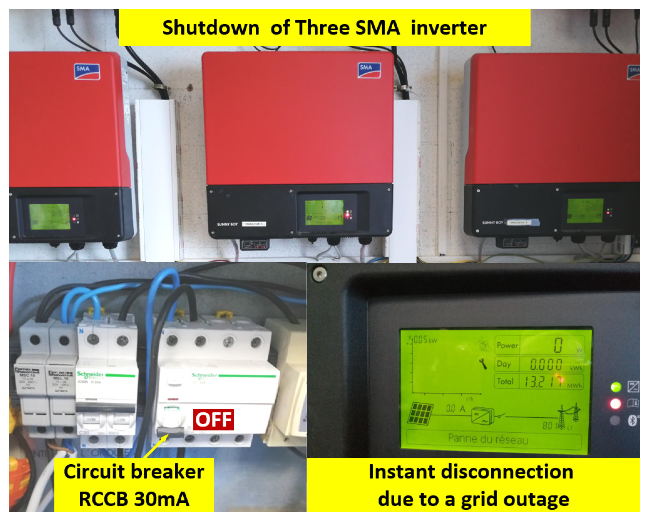
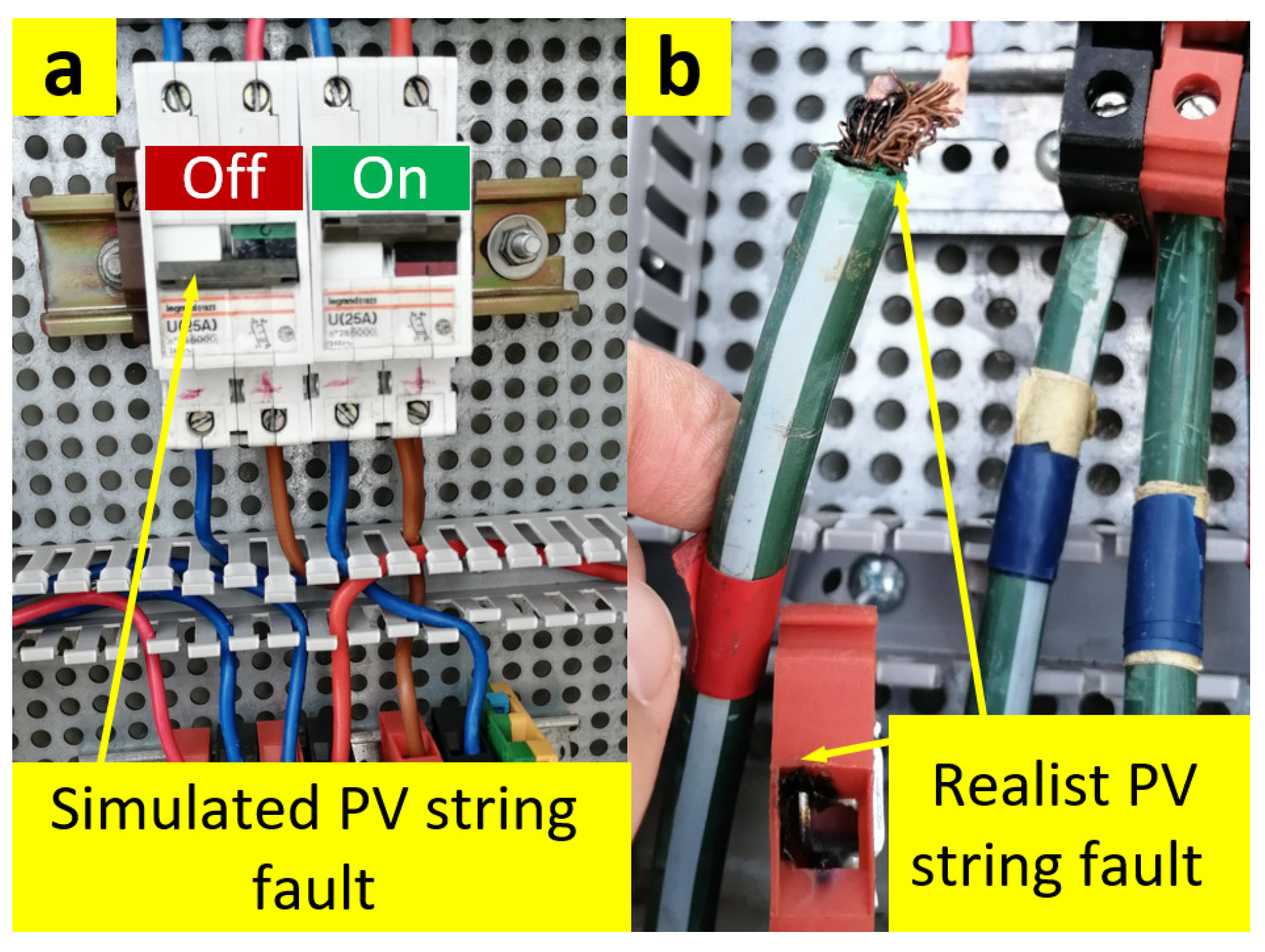
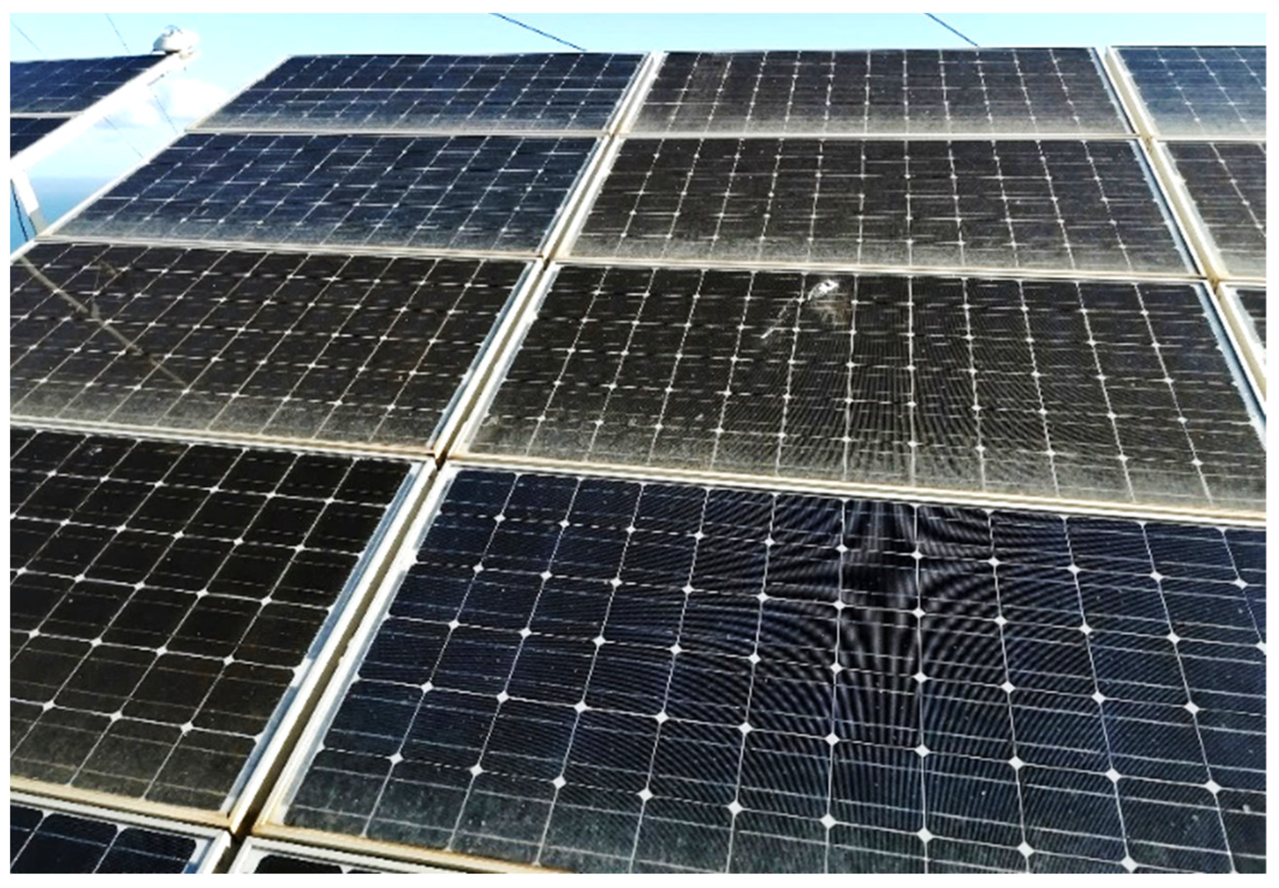
Anomalies and faults in PV installations can degrade their performance severely. Broadly speaking, faults in PV systems can be categorized based on their side of occurrence: Alternating Current (AC) or Direct Current (DC) in the PV installation [7,8]. Most DC side faults are located in PV array (e.g., partial shading and soiling effects, power degradation, DC wiring losses, mismatch of PV strings, electrical arc, line-line, and line to ground faults). Other faults in DC side are due to the rest of the Balance of System (BOS) components (e.g., cable, fuses, diodes, switches, and DC/DC converter). On the other hand, total black-out and grid outage are the two important faults occurring in the AC side. The grid outage faults are due to unstable voltage and lightning [9]. Detecting and classifying both DC and AC faults affecting PV systems are surely critical issues into be carefully addressed. To this end, various fault detection and diagnosis (FDD) procedures have been developed to detect and identify the type of fault in the DC or AC side of PV systems [10,11,12,13]. These techniques help to increase the system reliability and lifetime of PV installations.

The high efficiency nowadays needed for PV systems demands ongoing monitoring of the working condition of these systems [14,15]. Hence, reliable and precise FDD techniques able to provide the information needed to maintain optimum working conditions, are necessary to ensure (1) fast detection and accurate localization of faults, (2) reduce plant downtime, (3) extend long-term profitability (4) and exploit full power generation [16]. The International Energy Agency (IEA) Photovoltaic Power Systems Program (PVPS) has reported in [17] ten (10) on-site inspection techniques using mobile test equipment for PV modules and arrays. These techniques range from I-V characterization to imaging techniques used to detect and localize failures (e.g., electrical mismatch of PV strings, degradation, and cell cracks). For materials analysis, spectroscopic methods were also considered in [17]. In the last ten years numerous FFD methods have been proposed to accurately detect and identify faults in grid-tied PV systems [9,18,19,20].

FDD techniques in PV systems include two main categories: based on parametric models [21,22,23] and data-driven models [24,25]. Indeed, the parametric models are specified in terms of power, type, and size of the PV system installed. Therefore, parameter identification and model calibration are mandatory for each PV installation, which represents the weakness of these models. On the other hand, the advantage of non-parametric or data-driven approaches is the consideration of the PV system as a black box without parameterization but requires a lot of historical data to develop a behavioral model.

Data-driven approaches that rely on data collected from an inspected PV system to achieve outstanding performance have become appealing due to the availability of big data [26,27,28]. Data-driven fault detection methods such as Gaussian process regression-based charts [26], ensemble learning [28], artificial neural network methods [29,30,31,32,33], and deep learning [34], have received considerable attention in recent years due to their capability to automatically extract relevant features from high-dimensional data. For instance, in [28], a method based on ensemble learning models (i.e., Boosting and Bagging) is proposed to identify faults in the DC side of a PV system. Here, Bayesian optimization method is utilized to calibrate the hyper-parameters of the ensemble learning models in the training stage. After these models are employed as residual generators, the double exponentially weighted moving average (DEWMA) chart is applied to the generated residuals for fault detection purposes. In [26], kernel-based regression models (i.e., gaussian process regression and support vector regression) are used to model the nominal behavior of the inspected PV plant and the k-nearest neighbors-based detector is employed to discriminate between healthy operation and faulty conditions. Such an approach employs kernel density estimation to determine the detection threshold in a nonparametric way, which extends the flexibility and applicability of this approach.

Alternatively, model-based FDD techniques are based on the comparison between the measured data and the prediction from a mathematical model. The analytical model is often established based on some fundamental understanding of the PV system under normal operation states. In the past two decades, the interest in using model-based methods for FDD by engineers was high due to their mathematical and systematic characteristics. Model-based approaches include the empirical models [35,36], the one-diode model [37], and the two-diodes model [38]. Other approaches use the Kalman filter [39], Fourier series [40], and thermoreflectance imaging [41,42] to detect and recognize faults occurring in PV systems. Essentially, in the model-based methods, residuals, which are the deviation separating the measurement from the model predictions, are employed as indicators of faults in the inspected PV systems [43]. Hence, residuals are for fault detection and diagnosis. This study is within a model-based FDD framework.

Recently, the IEA-PVPS Task 13 in [44] has reported a benchmarking study of numerous approaches for computing the performance loss rates (PLR) of commercial and research PV system in different climatic zones. The PLR method is used by solar PV power plant owners, investors, and operators to estimate power output of a PV system over its service life. Therefore, discrepancies in different calculation methods can have a significant impact on the electricity generation cost. The benchmarking study is critical due to the inconsistency in reported PLR results based on the many methods currently used to compute the PLR of PV systems.

In the literature, many installed PV systems use analytical monitoring and performance analysis to avoid economic losses due to malfunctions problems [45]. For example, the study in [46] presented an automatic supervision and Fault Detection procedure on the DC side of the PV systems, analyzing both power losses and deviation of the DC current and DC voltage under the MATLAB/Simulink environment. An evaluation of the current indicator (Ci) and voltage indicator (Vi) at maximum power point (MPP) for automatic detection of main faults occurring in the PV systems was performed in [47]. This method is simple and can be integrated into the inverter for real-time supervision of the PV system. In [48], a level online FFD technique based on power losses analysis (PLA) for solar PV systems was proposed. The work in [49] presents remote supervision and fault detection and identification (FDI) of grid connected PV (GCPV) systems using the PLA method through the open platform communications (OPC) technology-based monitoring. In [50], an online monitoring FDI technique is introduced based on Vi analysis allowing for a reduction of the number of the sensors using power line communication (PLC), with an economic analysis of GCPV systems. In [51], two faults indicators, named voltage ratio (VR) and power ratio (PR) are defined to determine the fault type, time, and location of failure. A review of the main strategies for automatic FDD based on PLA at the AC side and both Ci and Vi at the DC output of the PV array is reported in [52]. In [53], an FDD method based on the evaluation of voltage and current indicators was employed to identify faults of the PV array. Even under various climatic conditions, this method is able to distinguish between degradation, permanent shading, and temporary shading faults.

A model-based FDD method was proposed in [54] which combines (1) the physical and statistical models and (2) fault diagnosis based on the physics of each failure. Both approaches contribute to optimizing the operation and maintenance of PV plants. The FDD capabilities of this method have been verified in a case study using six years of Supervisory Control and Data Acquisition (SCADA) data from a 315 kWp PV system. The study in [55] presents an effective approach to detecting and identifying various faults in PV systems, including short and open-circuit faults, inverter disconnection, and partial shading conditions. Toward the end, three indicators are used to give information on the state of the PV system regarding normal and faulty operation. In the literature, few studies exploit satellite data instead of on-site data measurements to estimate PV energy production. In [56], the satellite-derived solar irradiance data were analyzed by the PLA method to remotely detect failures in a PV system. Recently, authors in [57] have proposed an FDD approach for detecting PV underperformance and accurately identifying and distinguishing the different fault types (e.g., inverter faults, degradation, snow, and soiling) in large-scale PV plants. The proposed approach was evaluated using historical data of one inverter from a 1.8 MWp PV plant. This method focuses on the differentiation of faults performance loss ratio based on statistical analysis to extract significant changes in time series data. Moreover, this method makes it possible to plan the cleaning event by quantifying the soiling level on the modules, and it also allows estimating the degradation rate of the installed PV modules. The key advantage of the automatic FDD method based on real-time difference measurement (RDM) is that it can practically identify the common faults in the PV array. The implementation is easy with minimal required components, the detection time is improved and the FDI accuracy depends on the fixed threshold limits from the behavior PV model. Despite the rather low degree of complexity of the RDM techniques, the measured data obtained during faulty conditions was necessary for better validation.

In this paper, we present an efficient technique merging both parametric models and performance loss rate (PLR) analysis to sense and recognize anomalies occurring in a GCPVS. The considered parametric models are accurate, easy to implement in real-time monitoring tools, and with low computational costs. Knowing that the precision of model-based techniques relies on the measurement’s quality and the model calibration method, main benefit of the proposed technique resides in its capability in detecting different types of anomalies in both DC and AC sides of a GCPVS. 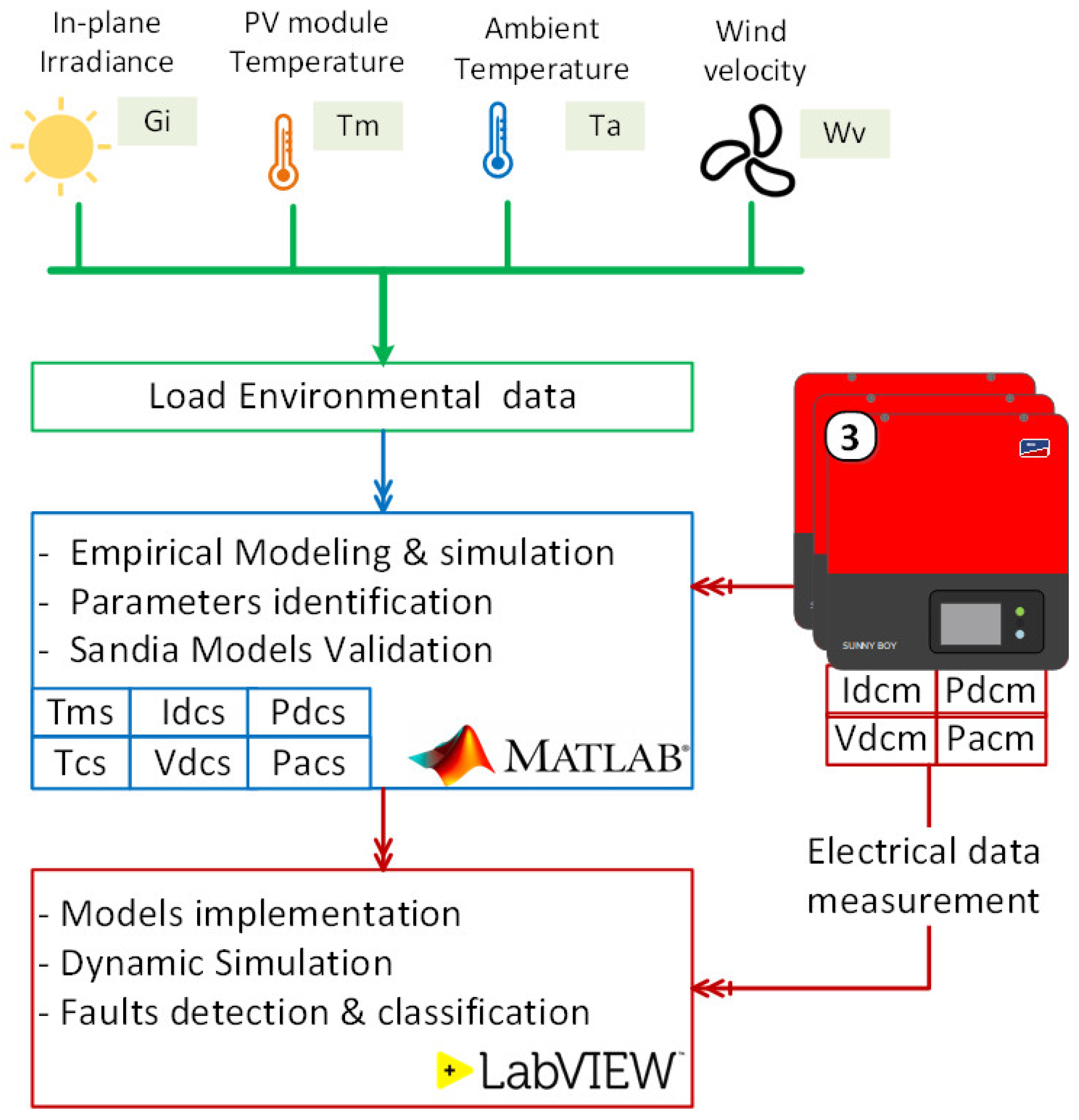Figure 1 illustrates the general framework of the proposed simulation process of behavioral modeling and fault diagnosis of the GCPVS using MATLAB and LabVIEW. The main contributions of this work are recapitulated as follows.

• At first, we introduced a parametric approach to model the behavior of the inverter and the PV array based on Sandia National Laboratories (SNL) empirical models to estimate the electricity production and analyze the performance of the inspected GCPVS. More specifically, the parametric models were validated and calibrated under MATLAB using experimental data. Sandia models have been implemented under LabVIEW to design a user interface for dynamic simulation of the GCPVS.
• Furthermore, this study introduced a simple and effective diagnostic tool to uncover and identify anomalies in a PV system. To this end, the residuals were calculated with the already calibrated Sandia parametric models. Then, the examination of the residual is conducted by analyzing the Performance Loss Rates (PLR) of four electrical indicators (i.e., DC voltage, DC current, DC power, and AC power). The effectiveness of the presented FDD methods is demonstrated on real data from a 9.54 kWp grid-connected PV system. Various anomalies were investigated in this paper, such as partial shading, soiling on the PV array, and DC/AC efficiency faults. Results showed the capability of the proposed FDD technique to provide significant help for PV system monitoring.
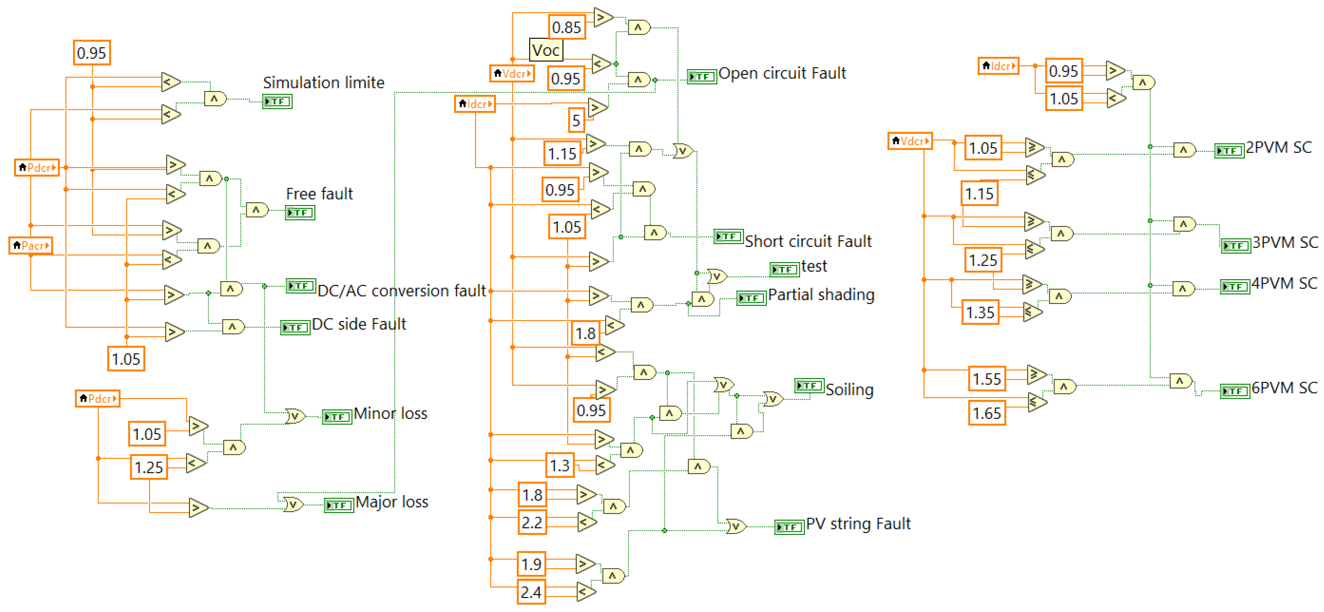
• Finally, the developed FDD strategy with threshold limits for each fault was integrated into the supervision interface under LabVIEW. The investigated faults were successfully detected and identified.

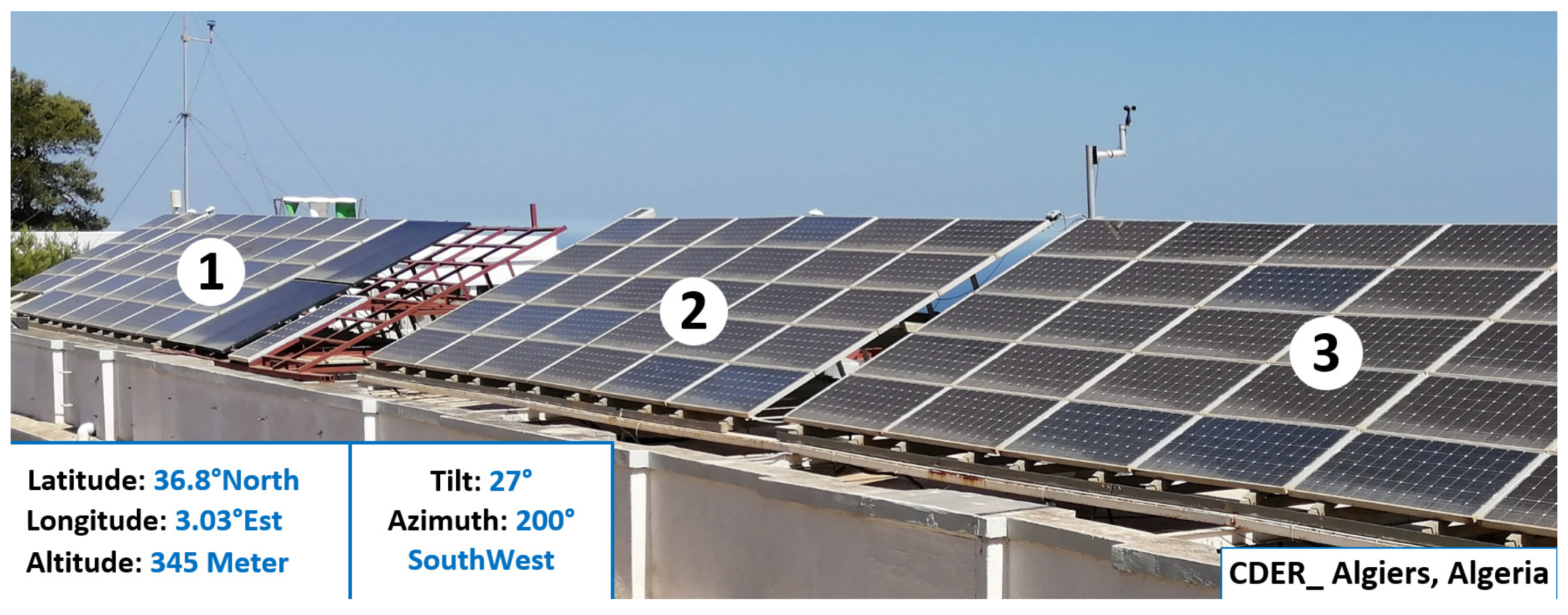
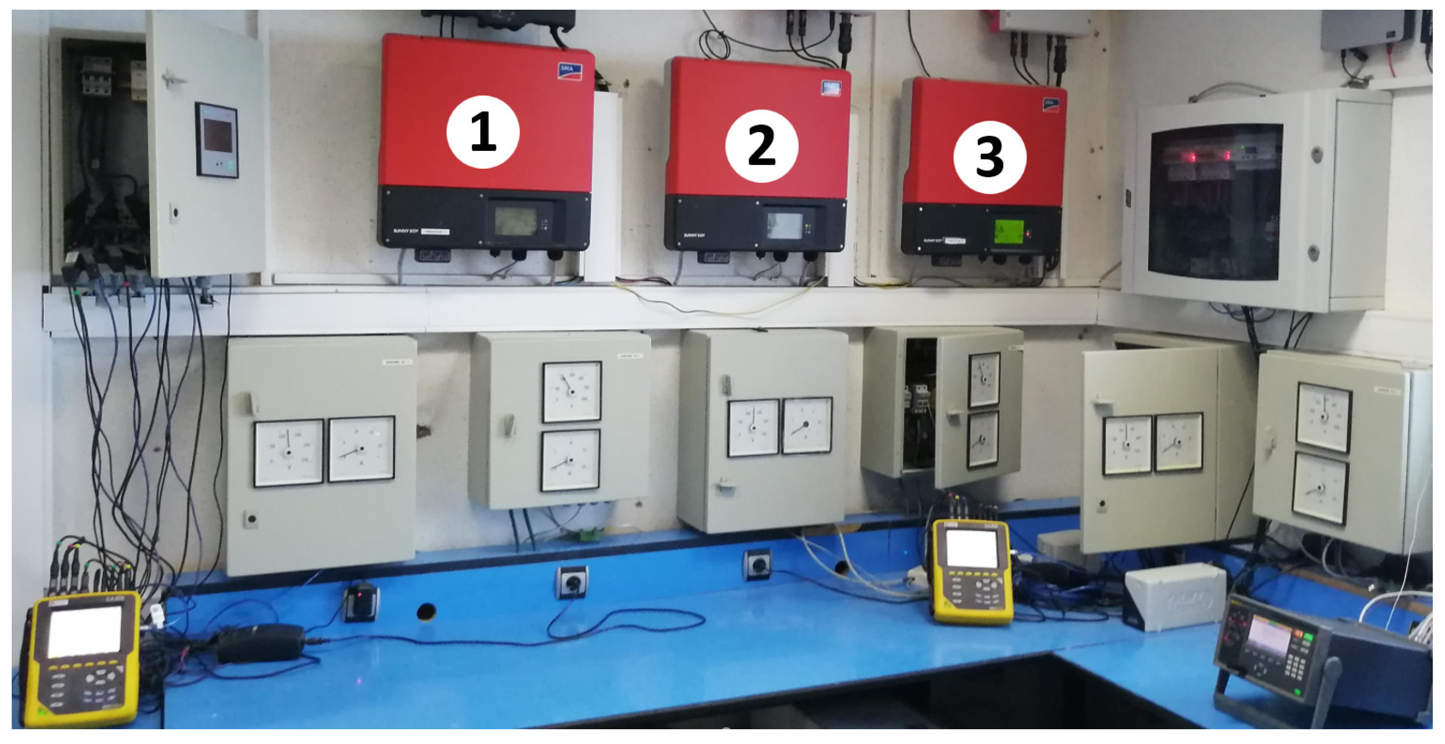
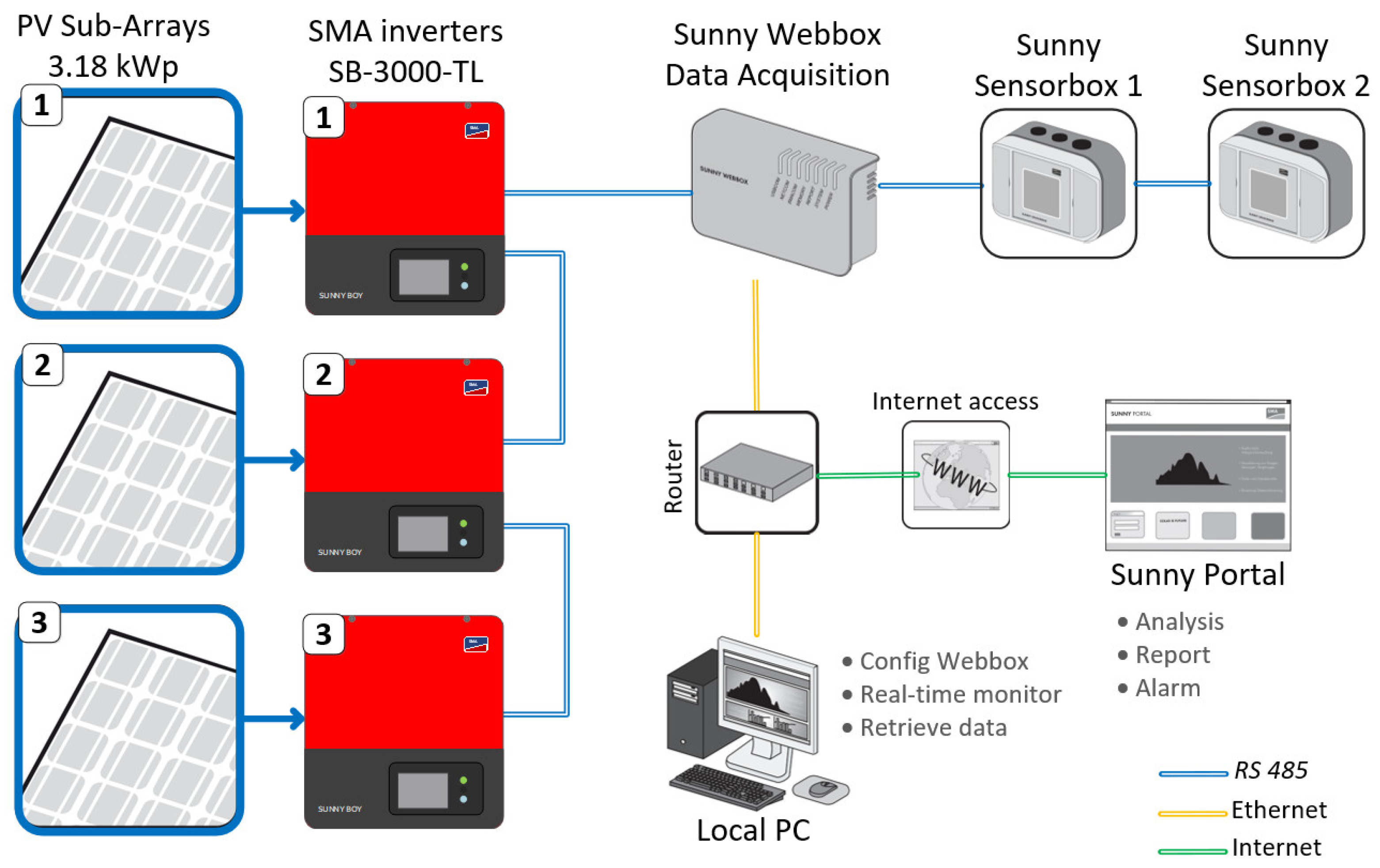
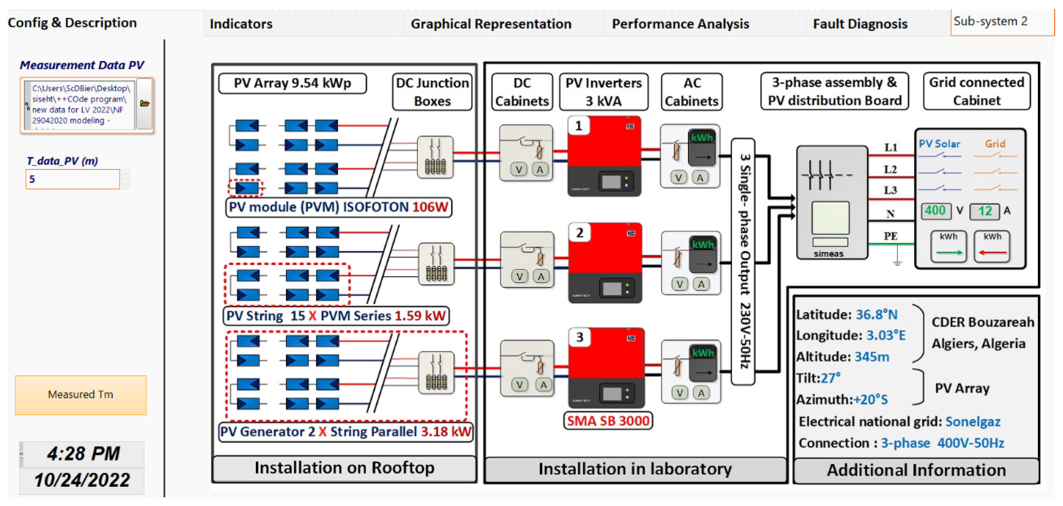
This work is organized as follows. Section 2 is devoted to the description of the used grid-tied PV system. Then, Section 3 presents the investigated parametric models for PV system modeling. Section 4 briefly describes the proposed PLR-based FDD method and discusses the experimental results. The last section includes this study and provides some future directions.

2. Description of Grid Connected Rooftop PV System

In this paper, we use the experimental data collected from the Grid-Connected PV System (GCPVS) to validate the performance of empirical model and the proposed FDD method. Indeed, the normal or fault-free data are used to validate the parametric models, which emulate the electrical behavior of the PV array and the PV inverter. On the other hand, the faulty data were used to develop and test the proposed FDD method.

The GCPVS illustrated in Figure 2 is composed of 90 PV modules with a peak power of 9.54 kilowatts (kWp) in operation for more than 18 years. The entire PV array is divided into three sub-arrays of a 3.18 kWp each, the sub-array is composed of two parallel strings of 15 PV modules (PVM) in a series. The main electrical characteristics of the PV module (Isofoton I106-12, Isofoton, Málaga, Spain) and PV Sub-array at standard test condition (STC) are given in

Table 1. Main electrical specification of PV Module (Isofoton I106-12) and PV sub-array at standard test condition (STC).

Parameters	PV Module	PV Sub-Array
Short circuit current ISC (A)	6.54	13.08
Open circuit voltage VOC (V)	21.6	324
Current at MPP IMPP (A)	6.1	12.2
Voltage at MPP VMPP (V)	17.4	261
Maximum power PM (W)	106	3180

MPP signifies the maximum power point.

. As illustrated in Figure 3, the GCPVS is composed of three similar single-phase PV sub-systems connected to low-voltage grid [58]. All PV sub-system consists of (1) PV sub-array, (2) grid-tie inverter (SMA Sunny Boy 3000), and (3) electrical cabinets for protection on DC and AC sides.

Table 2. Main electrical specification of the installed grid-tie Inverter (SMA Sunny Boy-3000).

Parameters	Nominal AC Power Output	Range of Input DC Voltage	Inverter Efficiency	Allowed Range of AC Voltage	Allowed Frequency Range
Values	3000 W	175–500 V	96.3–97%	180–280 V	49.5–50.5 Hz

gives the main electrical specification of the PV inverter SMA SunnyBoy-3000TL-21.

Description of Turnkey Monitoring System Provided by SMA

Nowadays, most grid-connected photovoltaic inverters are equipped with a monitoring system, which is an important tool for supervising the performance of PV installations [59]. Without a reliable and accurate monitoring system, it is difficult to know if a PV installation is operating properly or needs some maintenance. As shown in Figure 4, the monitoring of the PV installation is assured by SMA sunny Webbox data acquisition [60] via RS485 protocol, allowing to communicate with SMA sunny Sensorbox in order to measure the environmental parameters (i.e., titled irradiance, temperature of PV module, ambient air temperature, and wind velocity).

The electrical data of three PV sub-systems in both DC and AC sides are retrieved from internal measurement of grid-tie inverters using SMA WebBox [61]. The sampling time is about 10 s for all measured parameters, which is sufficient for analytical monitoring of the PV system according to IEC 61724 standard. The measured data were averaged and recorded every 5 min.

3. Modeling of Grid Connected PV System Using Parametric Models

The performance of PV installations depends on many parameters, including (1) weather conditions, (2) performance of the PV system components, and (3) grid parameters. Solar PV systems can be subjected during operation to various anomalies that affect their components (e.g., modules, cables, protections, or inverters) [6].

The behavioral simulation of the PV system connected to the grid makes it possible to create reference thresholds for the monitoring system carried out, which makes it possible to analyze the performance and the power losses in order to detect and identify the various faults affecting the PV system. The aim of the behavioral simulation of the GCPVS is to obtain the expected evolution of DC Power produced by the PV array as well as the AC power at the output of the PV inverter, considering real climatic conditions.

Here, the simulation of the GCPVS is based on the SANDIA parametric models that have been implemented and evaluated under the MATLAB environment. Here, aging and mismatch losses were included in the models using derates factors. Shading and soiling in a PV system are considered as anomalies, so they are not modeled. The appropriate selection of parametric models with good parameter estimation is the key to minimizing the error between measurement and simulation under normal operation of the PV system. The simulation of the grid-connected PV system allows obtaining the expected evolution of maximum DC power of the PV array, as well as the AC power at the inverter output, taking into account the real weather conditions.

3.1. Sandia PV Array Performance Model

The behavioral model of a PV module depends on the many electrical and meteorological parameters. The Sandia PV Array Performance Model (SAPM) is presented by the following equations below.

3.1.1. Cell and Module Temperature Models

Following the proportional relationship, between the voltage of the module and its temperature, an accurate estimation of the cell temperature allows a good prediction of the voltage behavior. The PV cell or module temperature is usually obtained by prediction. To estimate the temperature of the PV cell/module, numerous models have been introduced in the literature [62,63,64,65,66].

• Module Temperature Model

To estimate back-surface module temperature ($T_{ms}$) in (°C), Sandia proposes an accurate model which depends on three parameters [35] (Equation (1)): irradiance incident on module surface or Plane of Array (POA) irradiance ($E_{POA}$) in (W/m²), ambient air temperature (T_a) in (°C), and wind velocity ($W_v$) in (m/s).

$$T_{ms}=T_a+E_{POA}·e^{s1+s2·Wv}$$

(1)

In (1), s1 denotes the empirically parameter creating the upper boundaries for module temperature at high tilted irradiance and low wind velocity, and s2 designates the empirical parameter defining the decrease rate in the module temperature value as a function of the increase in the wind velocity.

• Module to Cell Temperature Model

The Sandia model of PV cell temperature depends on the measured PV module temperature $(T_m)$, measured POA irradiance $\left(E_{POA}\right)$, and a temperature difference parameter between module and cell $(\Delta T)$, as represented by Equation (2).

$$T_c=T_m+\frac{E_{POA}}{E_0}·\Delta T$$

(2)

ΔT is a parameter that depends on the construction, materials, and mounting configuration of the PV module [67]. In the studied PV array, ΔT is fixed at 2 °C.

3.1.2. Effective Irradiance

Effective irradiance $\left(E_e\right)$ is the available plane of array irradiance with consideration of spectral mismatch, soiling accumulation on PV array, and angle of incidence losses. In a general sense, or it can be considered as the irradiance actually received by the PV cells before conversion to power. A simplified relation based on POA irradiance measured by pyranometers or reference PV cell is suggested in Equation (3).

$$E_e=\frac{E_{POA}}{E_0}·Sf$$

(3)

where $Sf$ is the soiling factor (=1 when clean).

3.1.3. DC Current Model

The sandia dynamic model [35] to estimate DC current of PV array at maximum power point (MPP) is expressed by Equation (4).

$$I_{mp}=p\cdot (I_{m{p}_{STC}}\cdot N_p\left(c_0{E}_e+c_1{E}_e^2\right)\cdot \left(1+cti\left(T_c-T_0\right)\right)).$$

(4)

where $I_{mp}$ is the DC current of the PV sub-array at the MPP (A), $I_{m{p}_{STC}}$ denotes MPP current of one PV module at standard test condition (STC) in (A), $p$ is the number of strings in parallel ($p=2$), $E_0$ is the reference solar irradiance (typically $E_0=$ 1000 W/m²), $T_c$ denotes the cell temperature inside module in °C, $T_0$ is the reference cell temperature ($T_0=$ 25 °C), $N_p$ is the number of cell-strings in parallel in module, $c_0$ and $c_1$ are the empirically determined parameters relating PV sub-array current to effective irradiance, equal to 1. Here $cti$ is the current temperature coefficient, equal to $2.3\mathrm{mA}/°\mathrm{C}$ in the datasheet, this coefficient has also been identified.

3.1.4. DC Voltage Model

The dynamic model of the estimated PV string voltage $V_{mp}$ at MPP is expressed by Equations (5) and (6). This model is based on sandia PV array performance model [35]. $V_{mp}$ is inversely proportional to the evolution of the effective cell temperature ($T_e$), and slightly proportional to the evolution of effective irradiance $(E_e)$.

$$V_{mp}=s\cdot \left(V_{m{p}_{\_STC}}+c_2{N}_s\cdot \delta \left(T_e\right)\cdot \mathit{ln}(E_e\right)+c_3{N}_s\left(\delta \left(T_e\right)\mathit{ln}(E_e\right){)}^2+\left(ctv\cdot T_e·E_e\right)-\left(cve/E_e\right))$$

(5)

with

$$\delta \left(T_e\right)=n\cdot k\cdot \frac{T_e+298.15}{q}.$$

(6)

where $V_{mp}$ is the voltage of PV string at MPP (V), $V_{mp\_STC}$ denotes the MPP voltage of PV module at STC (V), $T_e$ is the effective temperature of PV cell ($T_e=T_c-T_0)$, $s$ is the number of modules in series ($s=15$), $N_s$ refers to the number of cells in series in a module’s cell-string, and $k$ denotes the Boltzmann’s constant ($k$ = 1.38066 × 10⁻²³ (J/K)). Here, $q$ is the elementary charge ($q=$ 1.60218 × 10⁻¹⁹ (coulomb)), and $\delta \left(T_e\right)$ denotes the thermal voltage is related to the effective temperature of the PV cell $T_e$. Note that for the diode factor of unity ($n$ = 1) and a cell temperature of 25 °C, the thermal voltage is about 26 mV per cell. $c_2$ and $c_3$ are the empirically determined parameters relating voltage of PV string to effective irradiance, and $ctv$ represents the normalized temperature coefficient for MPP voltage, equal to $-74\mathrm{mV}/°\mathrm{C}$ in the datasheet, this coefficient has also been identified.

3.1.5. DC Power

The DC power at MPP is calculated by the following relationship

$$P_{mp}=V_{mp}‧ I_{mp}$$

(7)

3.2. Sandia Inverter Model

The second important component in a grid-connected PV system is the PV inverter, which allows the conversion of DC power to AC power in order to be connected to the AC grid with high efficiencies up to 99%. Here, to estimate the conversion of SMA sunny boy inverter, we have used an accurate inverter model developed by SNL [36]. This model is defined by the following equations.

$$P_{ACs}=\left\{\left(P_{ACo}/\left(A-B\right)\right)-C·\left(A-B\right)\right\} \left(P_{DCs}-B\right)+C·{\left(P_{DCs}-B\right)}^2$$

(8)

$$A=P_{DC0}·\left\{1+C_1·\left(V_{DCs}-V_{DC0}\right)\right\}$$

(9)

$$B=P_{S0}·\left\{1+C_2·\left(V_{DCs}-V_{DC0}\right)\right\}$$

(10)

$$C=C_0·\left\{1+C_3·\left(V_{DCs}-V_{DC0}\right)\right\}$$

(11)

The definition of the performance parameters is given below. $P_{ACs}$ is the predicted AC power based on predicted DC voltage (V) and DC power (W). $P_{DCs}$ denotes the estimated DC power at the inverter input, which equals to the maximum power of PV sub-array. $V_{DCs}$ refers to the simulated DC voltage of the PV sub-array at the inverter input, $P_{ACo}$ is the maximum AC power of PV inverter at Reference Operating Condition (ROC), $V_{DC0}\mathrm{and}{P}_{DC0 }$ represent respectively the DC voltage level and the DC power level at which rated AC power is reached under ROC, and $P_{S0}$ represents the DC power required to start the DC/AC conversion process. $C_0$ is the parameter that defines the curvature between AC power and DC power (1/W). $C_1$, $C_2$, and $C_3$ are the empirical parameters allowing respectively $P_{DC0}$, $P_{S0},$ and $C_0$ to vary linearly with DC voltage of PV sub-array at the inverter input, (1/V).

3.3. Parameters Identification

The identification of parameters using Artificial Intelligence (AI) techniques allows a good calibration of the empirical model with measured data. Note that the calibration of representative models is very important, in order to try to approximate the experimental reference data as much as possible and to accurately emulate the electrical behavior of the PV array and PV inverter in the PV system.

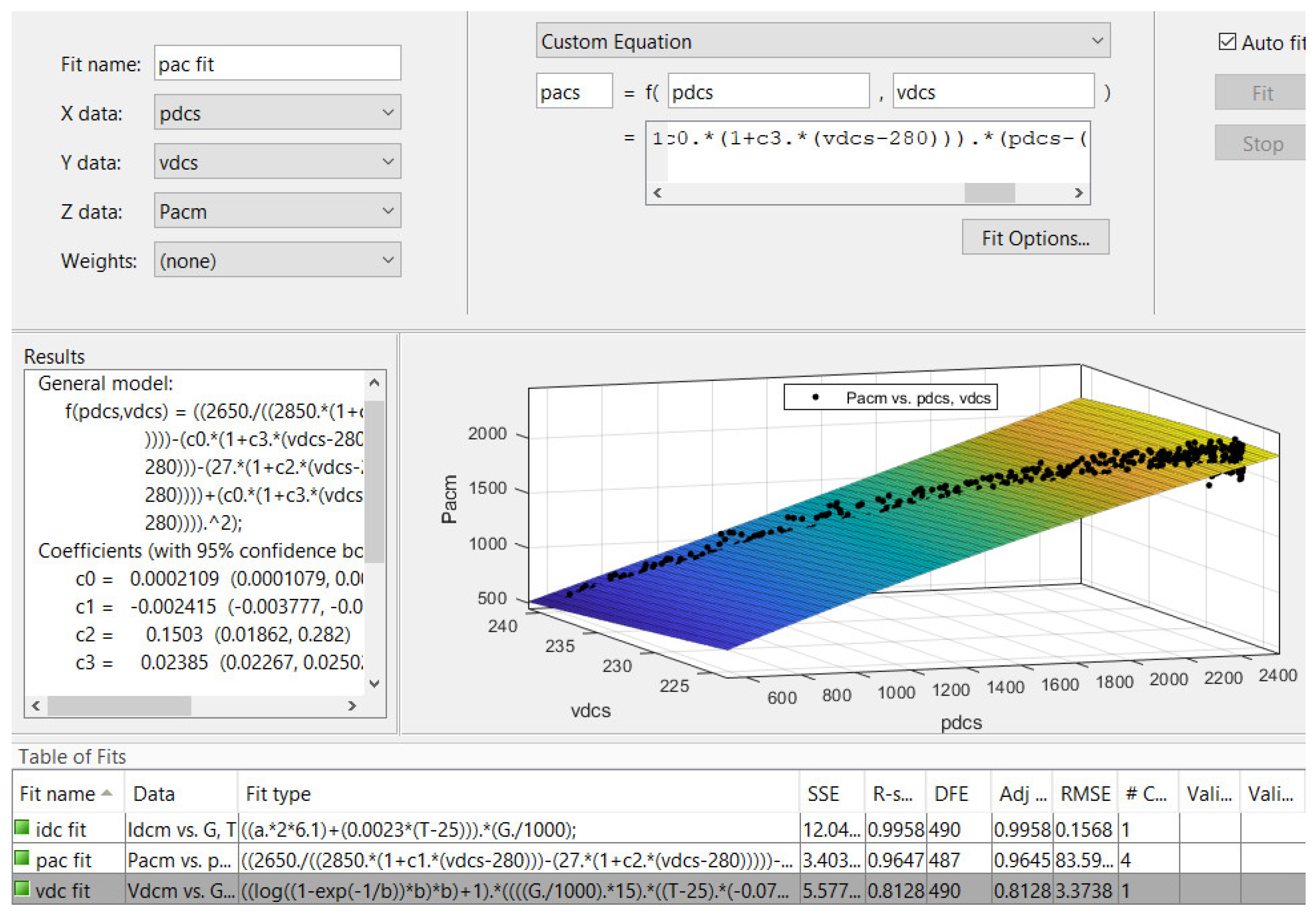
These models are built using normal data (i.e., without any anomaly and fault) and will generate residuals for real-time data to initiate the fault diagnosis process. Here, the parameters of the PV sub-arrays model and the inverter model were identified using a curve fitting toolbox under MATLAB software, where the fitting is based on the nonlinear least squares method and trust-region algorithm (Figure 5). In addition, the empirical models were validated and proved using experimental data collected from 9.54 kWp GCPVS under normal operating condition without faults and anomalies.

Three representative statistical indicators are considered to assess the prediction performance and accuracy of behavioral models: the mean absolute error (MAE), root mean square error (RMSE), and coefficient of determination ($R^2$). These metrics are computed as follows:

$$MAE=\frac{1}{n}{\sum }_{i=1}^n\left|Y_i-\widehat{Y_i}\right|,$$

(12)

$$RMSE=\sqrt{\frac{1}{n}{\sum }_{i=1}^n{\left(Y_i-\widehat{Y_i}\right)}^2},$$

(13)

$$R^2=1-\frac{{\sum }_{i=1}^n{\left(Y_i-\widehat{Y_i}\right)}^2}{{\sum }_{i=1}^n{\left(Y_i-\overline{Y}\right)}^2},$$

(14)

where $Y_i$ is the actual values, $\widehat{Y_i}$ denotes the estimated values, $\overline{Y}$ refers to the mean value of $Y_i$, and n is the samples number.

The empirical models used to estimate the temperature of the module back-sheet surface are function of three variables (i.e., POA irradiance, ambient air temperature, and wind velocity). Therefore, we used the procedure given in [68] to decompose the temperature model equation into two equations in order to estimate the coefficients using the curve fitting toolbox.

Table 3. Empirically identified parameters used to predict module back surface temperature using sandia model.

Coefficient	$\mathit{s}1$	$\mathit{s}2$
Values	−3.691	−0.08396

gives the identified parameters used to predict module back surface temperature. The empirically identified parameters used in order to predict DC current and DC voltage at MPP based on SAPM are given respectively in

Table 4. Empirically identified parameters used to predict DC current using sandia model.

Coefficient	${\mathit{c}}_0$	${\mathit{c}}_1$	$\mathit{c}\mathit{t}\mathit{i}$
Sub-array 1	0.961	−0.111	0.001
Sub-array 2	0.9828	−0.1338	0.001
Sub-array 3	0.9521	−0.1074	0.001

and

Table 5. Empirically identified parameters used to predict DC voltage using sandia model.

Coefficient	${\mathit{c}}_2$	${\mathit{c}}_3$	$\mathit{n}$	$\mathit{c}\mathit{v}\mathit{t}$	$\mathit{c}\mathit{v}\mathit{e}$
Sub-array 1	0.1239	4.292	2.442	−0.0731	0.3758
Sub-array 2	0.105	1.42	3.648	−0.07744	0.2891
Sub-array 3	0.1317	3.155	2.584	−0.07403	0.302

for three sub-arrays.

Table 6. Empirically identified parameters used to predict AC power using sandia inverter model.

Coefficient	${\mathit{P}}_{\mathit{S}0}$	${\mathit{V}}_{\mathit{D}\mathit{C}0}$	${\mathit{P}}_{\mathit{D}\mathit{C}0}$	${\mathit{P}}_{\mathit{A}\mathit{C}0}$	${\mathit{C}}_0$	${\mathit{C}}_1$	${\mathit{C}}_2$	${\mathit{C}}_3$
Inverter 1	15	269.8	2715	2574	−2.011 × 10−5	0.00168	0.4418	0.1339
Inverter 2	15.15	275.7	2770	2580	−4.172 × 10−6	0.001387	0.3327	0.3249
Inverter 3	15	262	2743	2563	−1.11 × 10−5	0.003248	0.7455	0.3097

illustrates eight parameters that were identified for three inverters based on the Sandia inverter model.

3.4. Simulation Result under Matlab

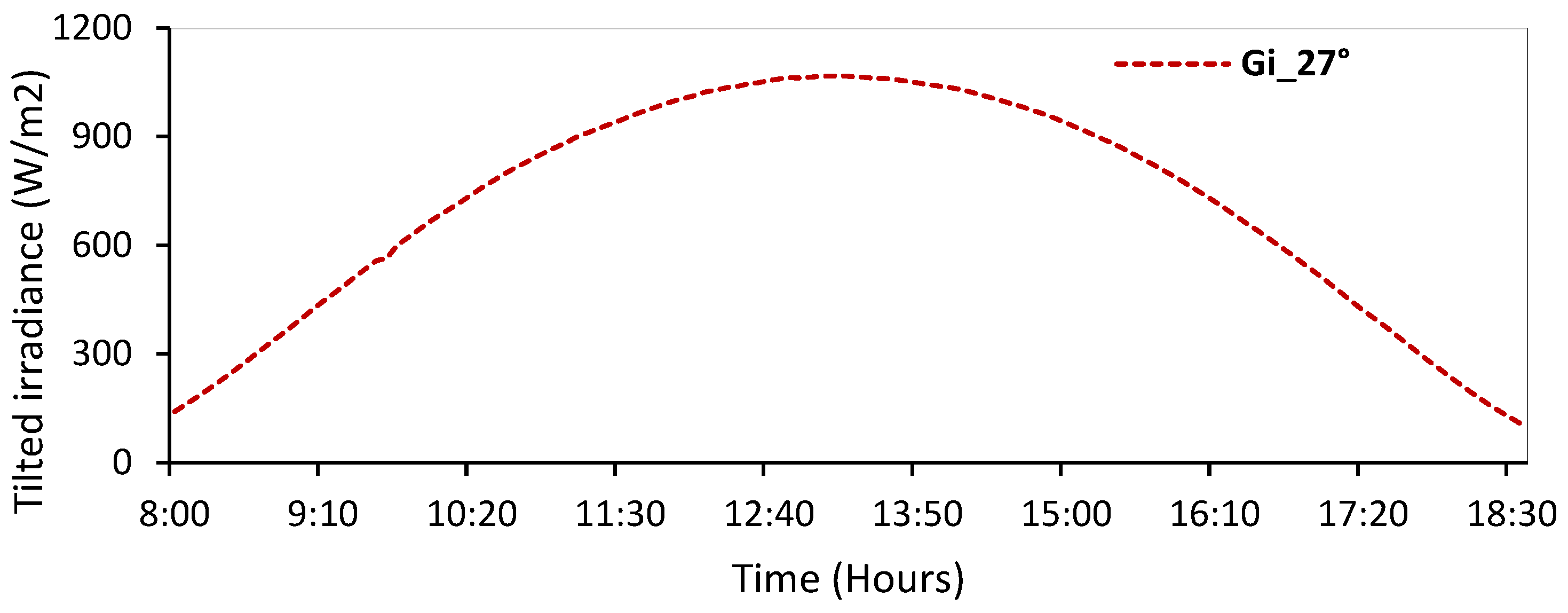
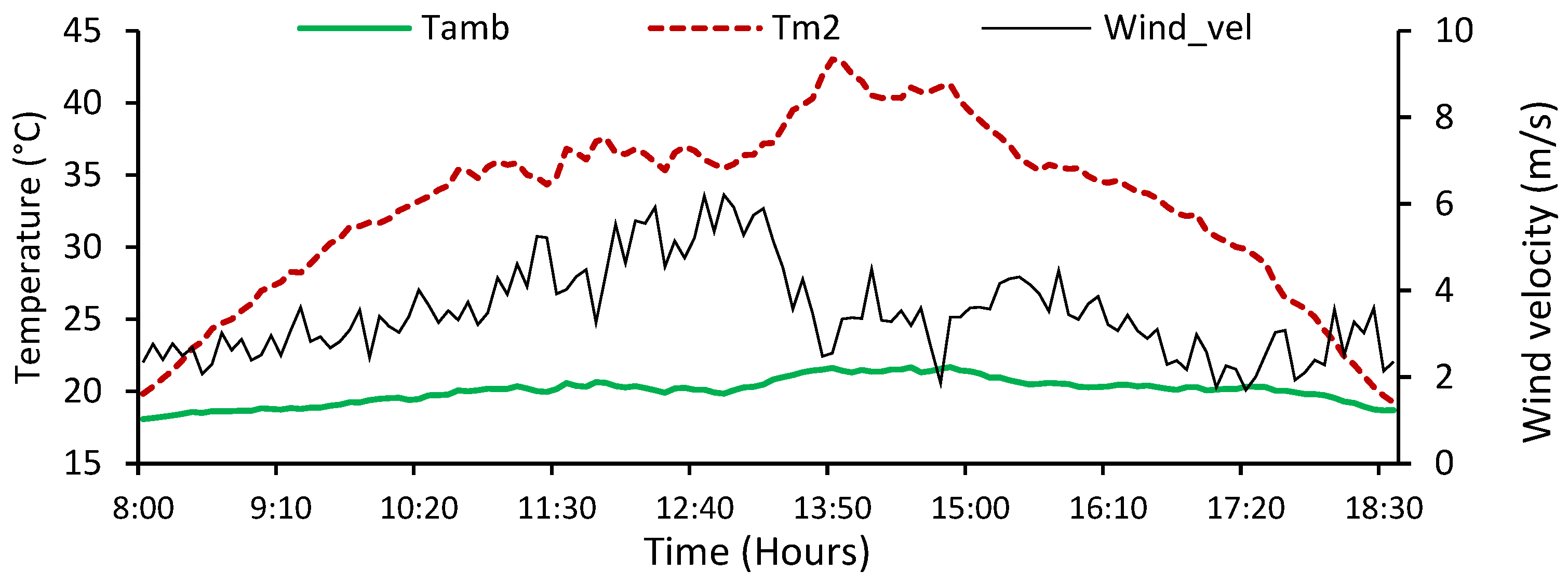
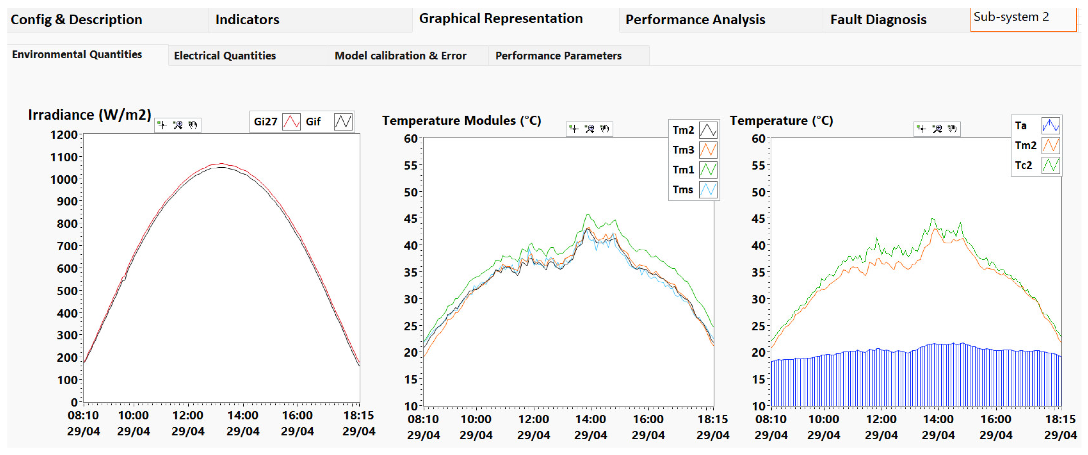
The simulation of all behavioral models was performed in the MATLAB environment. Before the simulation, all models were well calibrated using experimental data for a reference day with the following conditions: clear sky day, medium ambient temperature, and without (1) measurement faults, (2) shading, (3) significant soiling, and (4) electrical fault or other anomalies. Figure 6 and Figure 7 display the measured meteorological data used as input for DC current and DC voltage empirical models.

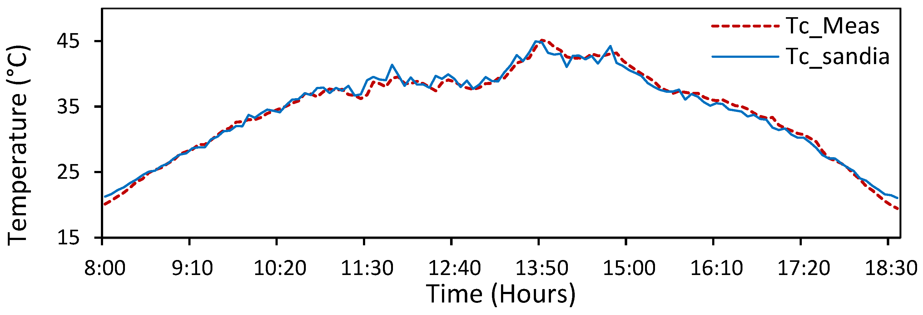
Figure 8 illustrates the measured PV cell temperatures of and predicted from four models. The measurements of effectiveness for the used PV cell temperature models listed in

Table 7. Regression metrics for the used Sandia PV cell temperature model.

Metrics/	MAE	RMSE	MAE (%)	RMSE (%)	R-Squared
Values	0.61698	0.77446	1.3811	1.7336	0.98589

confirm its good prediction performance.

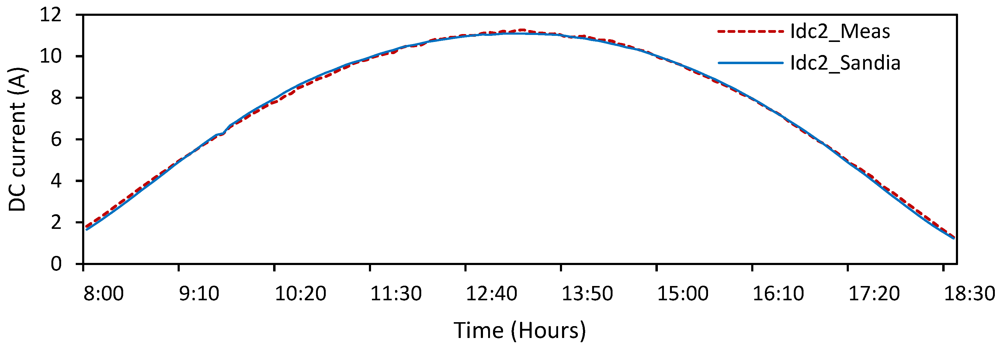
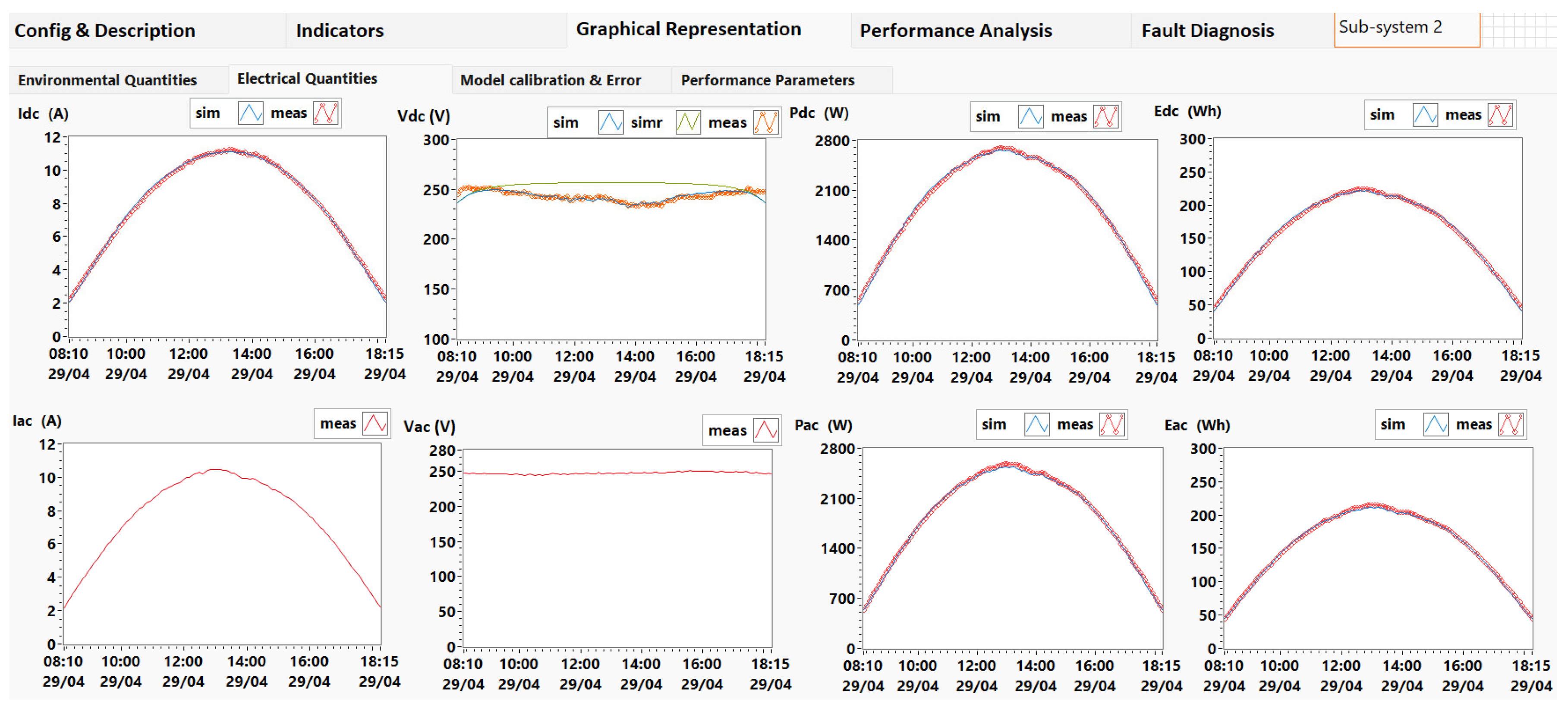
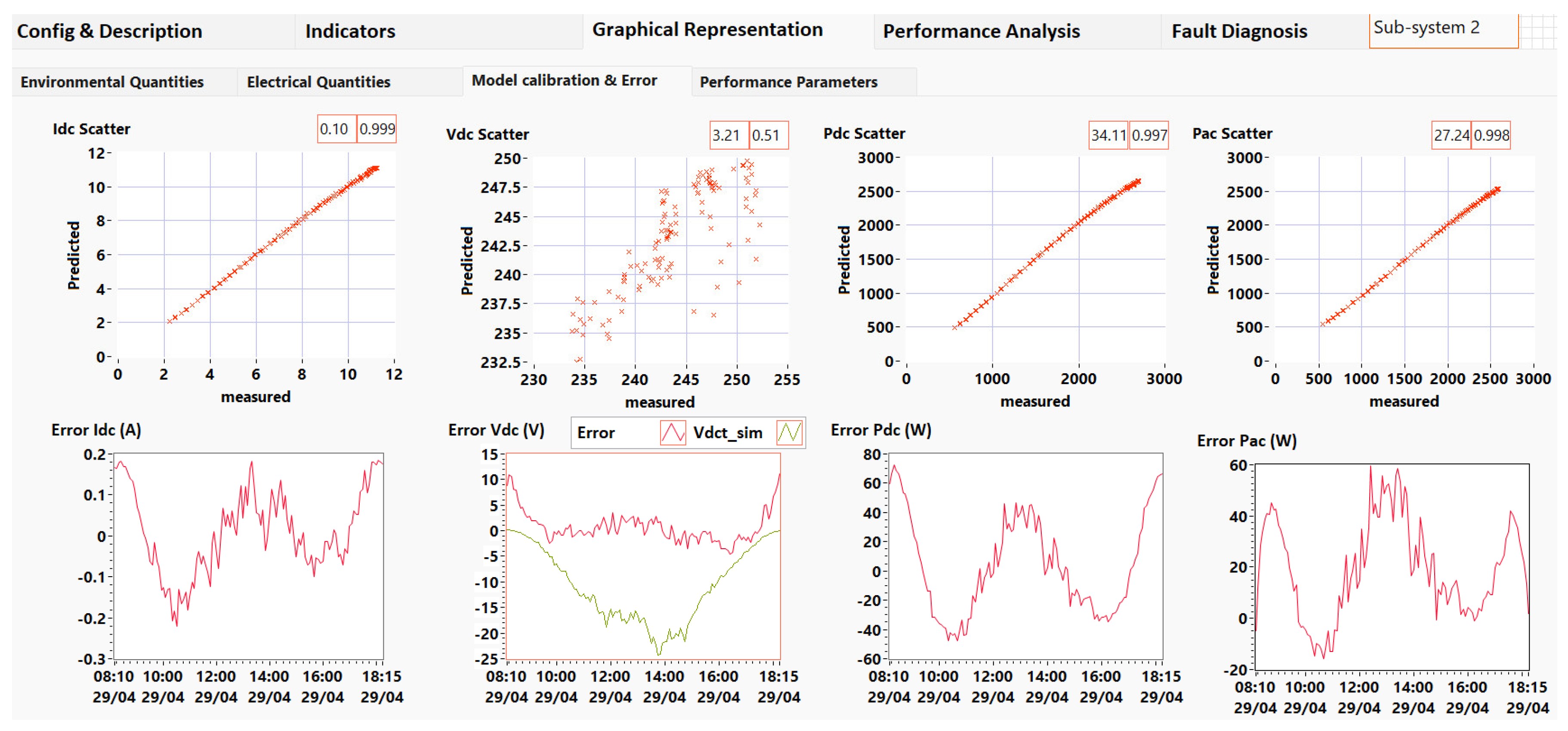
According to the regression metrics listed in Table 7, the Sandia model of module temperature shows good performance. For the simulations results by way of example, we are satisfied to give just the plots of sub-system 2, because the plots of sub-systems 1 and 3 look very similar to sub-system 2, the other sub-system will be compared in the regression metrics tables. Figure 9 shows the MPP current of the PV sub-array 2 measured and predicted for the DC current model.

Table 8. Regression metrics of DC current models simulated for three sub-arrays.

Metrics/Param.	MAE (A)	RMSE (A)	MAE (%)	RMSE (%)	R-Squared
Idc1	0.08	0.11	0.71	1.01	0.999
Idc2	0.09	0.10	0.76	0.92	0.999
Idc3	0.08	0.10	0.71	0.92	0.999

gives the regression metrics of the DC current model simulated for three sub-arrays. We can see a good agreement between the measured and the estimated data from models for all PV sub-arrays. The Sandia current is very accurate with $R^2$ around 0.999 for all PV sub-arrays.

Figure 10 shows the MPP voltage of sub-array 2 measured and predicted from the behavioral model.

Table 9. Regression metrics of DC Voltage models simulated for three sub-arrays.

Metrics/Param.	MAE (V)	RMSE (V)	MAE (%)	RMSE (%)	R-Squared
Vdc1	1.33	1.63	0.53	0.65	0.899
Vdc2	1.34	1.62	0.53	0.64	0.891
Vdc3	1.16	1.38	0.46	0.54	0.924

gives the regression metrics of the DC voltage model simulated for three PV subarrays. We can see a good fitting between the measured and the estimated data from the model for all subarrays. The $R^2$ is greater than 0.89 for three sub-arrays. We observe that for the predicted DC voltage the $R^2$ is low due to the sensitive variation of the DC voltage when tracking the maximum power point depending on the climatic conditions, while the RMSE is less than 0.66% for the Sandia model as shown in Table 9.

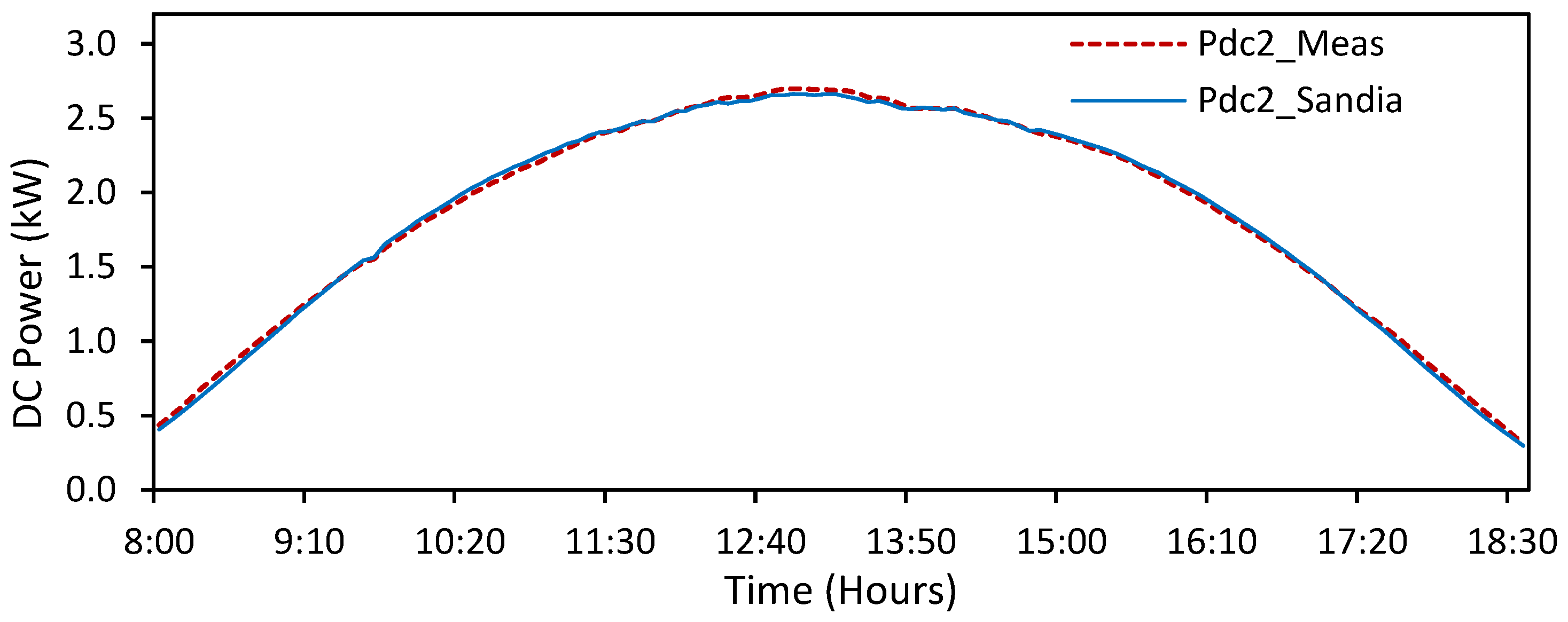
However, the DC power models using one equation are less accurate than models which are based on the product of DC current and DC voltage models. So, the DC power simulation results shown in Figure 11 are based on the product of the estimated DC current and DC voltage.

Table 10. Regression metrics of DC Power simulated for three sub-arrays.

Metrics/Param.	MAE (W)	RMSE (W)	MAE (%)	RMSE (%)	R-Squared
Pdc1	25.7	32.8	0.95	1.21	0.998
Pdc2	23.4	27.0	0.87	1.00	0.999
Pdc3	23.3	29.3	0.87	1.09	0.998

indicates a satisfying agreement between the measured data and the predicted value of DC power using both models (i.e., $R^2$ greater than 0.998). We notice that the simulation results of DC power are very close to those of DC current.

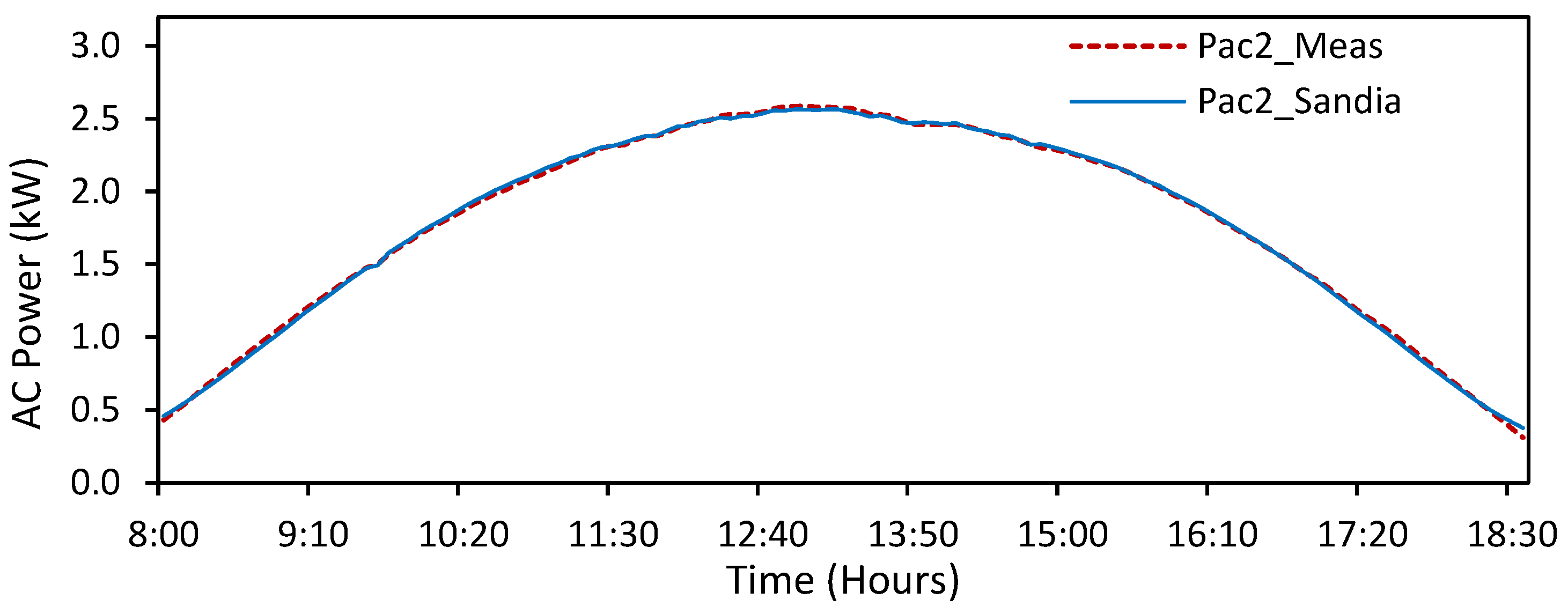
We also observe that the prediction of AC power using the Sandia inverter model, based on the predicted DC voltage and DC power, agrees very well with the measurement data as shown in Figure 12, with an $R^2$ greater than 0.999 and an RMSE that does not exceed 0.93% for the three simulated inverters (

Table 11. Regression metrics of AC Power model simulated for the three inverters.

Parameters	MAE (W)	RMSE (W)	MAE (%)	RMSE (%)	R-Squared
Pac1	18.9	24.1	0.73	0.93	0.999
Pac2	7.8	9.86	0.30	0.38	1.000
Pac3	17.2	24.0	0.66	0.92	0.999

).

In summary, the above-described empirical models fit well with the measured data.

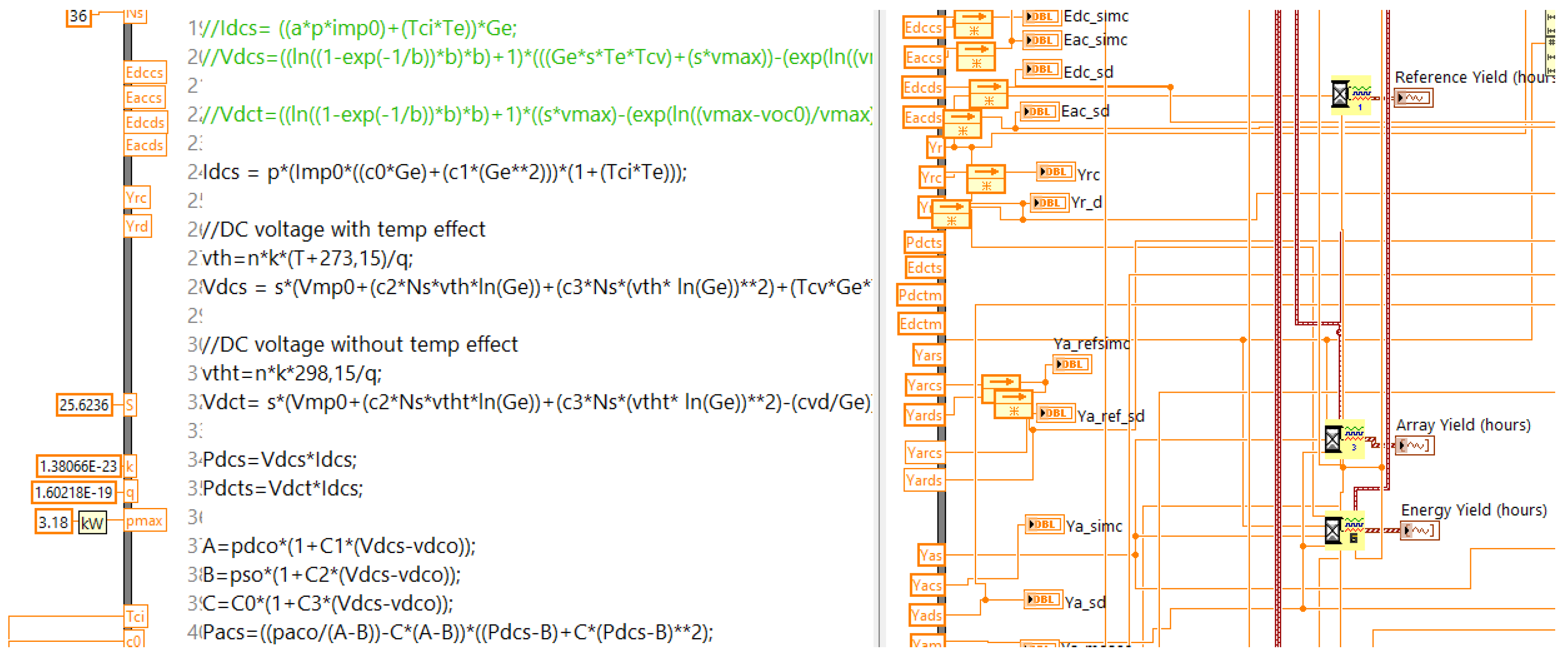
3.5. Model Implementation under LabVIEW

All behavioral models validated in MATLAB have been implemented under the LabVIEW code diagram using a graphical program combined with a textual program based on C language, this is called a virtual instrument (VI) (Figure 13).

The layout of the developed VI can be viewed in the front panel for an interactive user interface, including different tabs shown in Figure 14, Figure 15, Figure 16, Figure 17 and Figure 18.

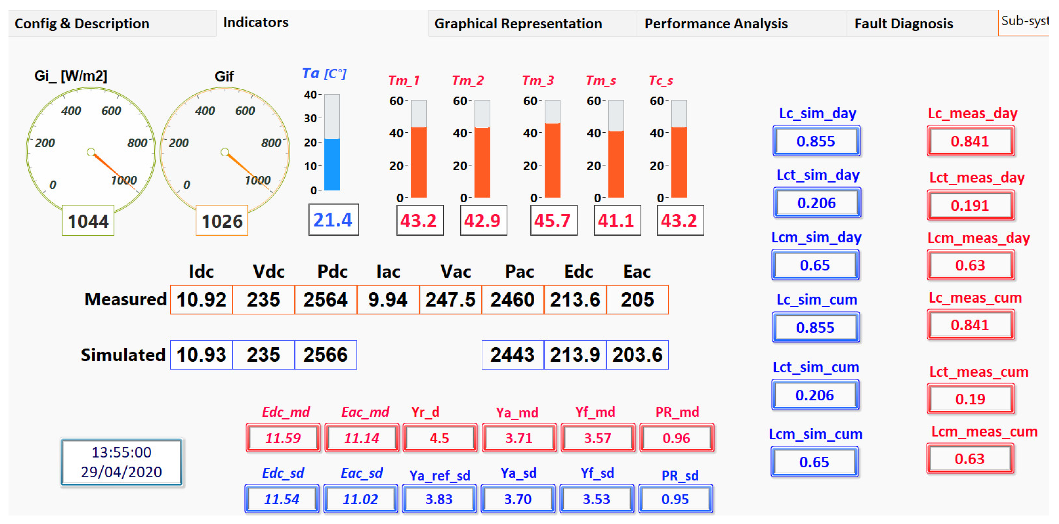
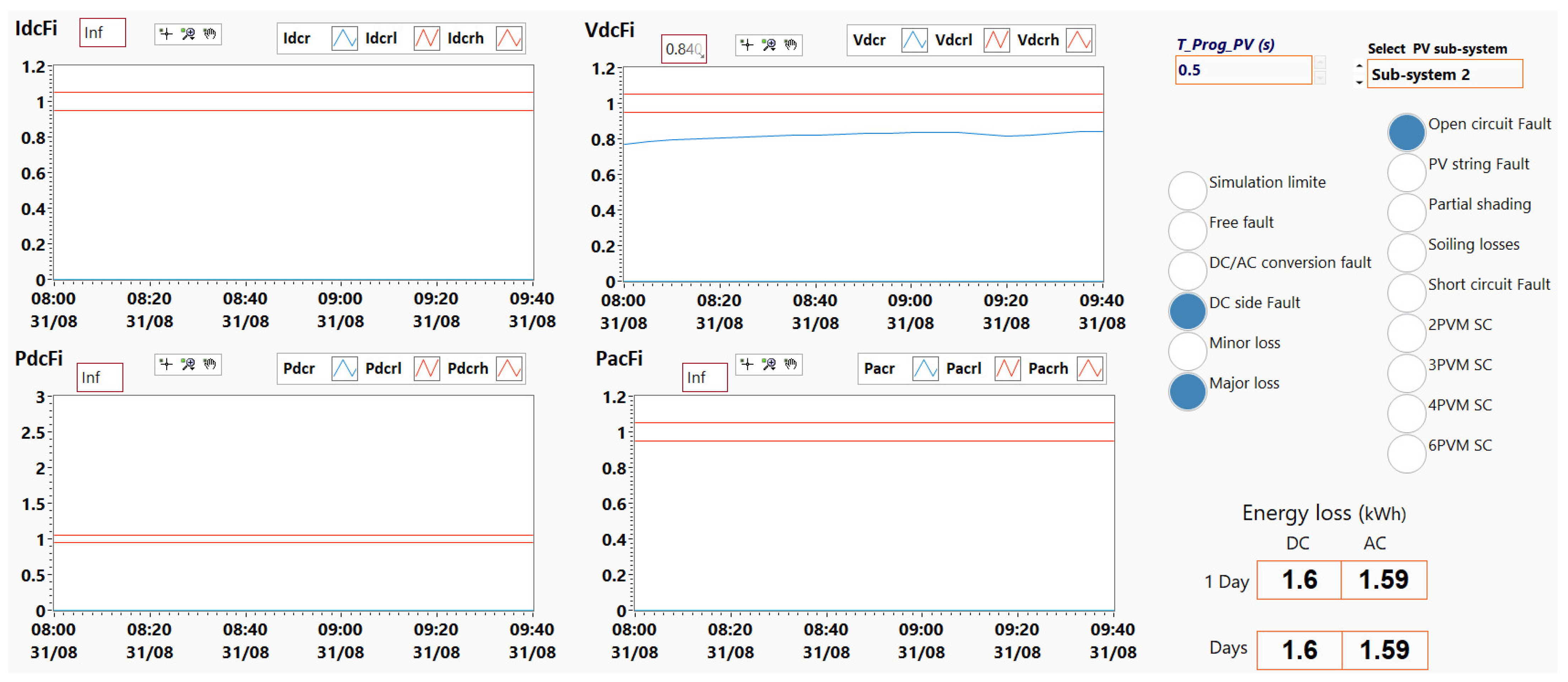
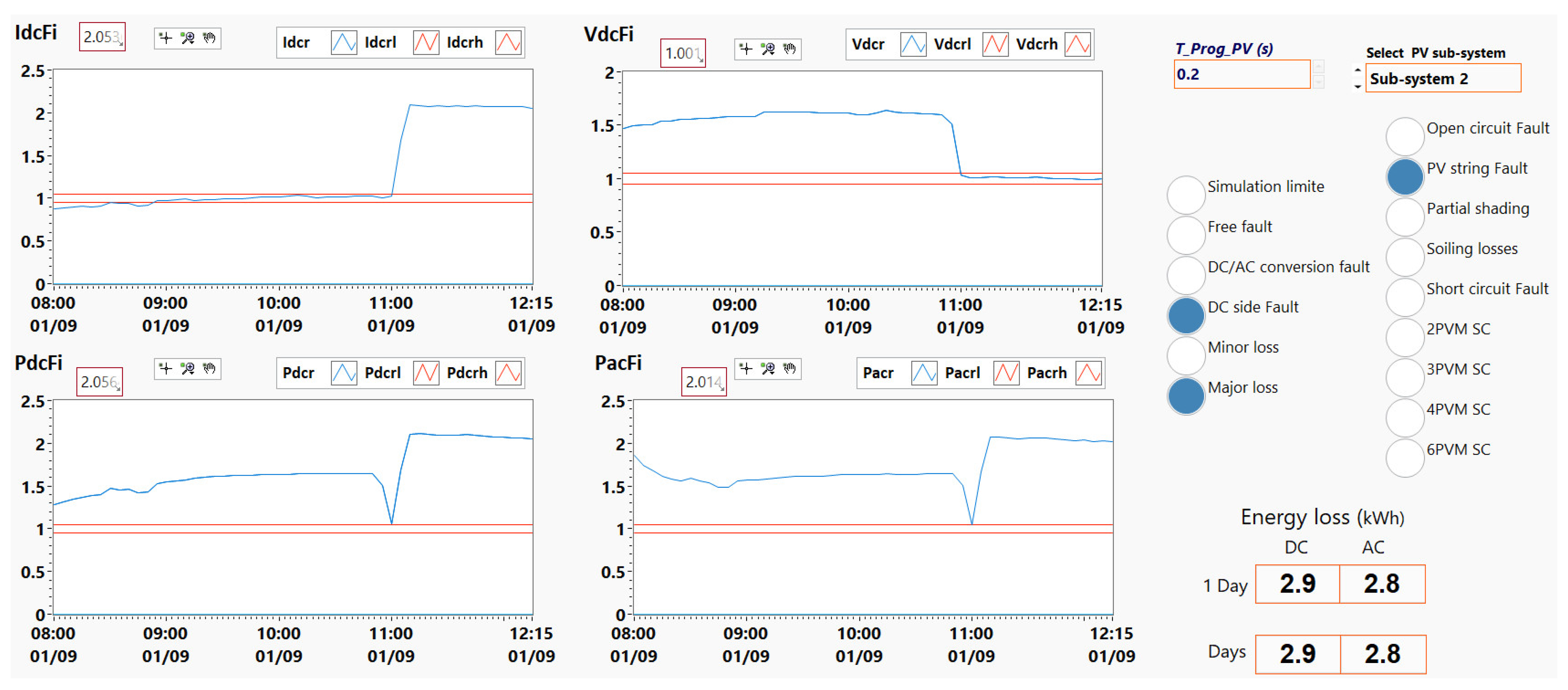
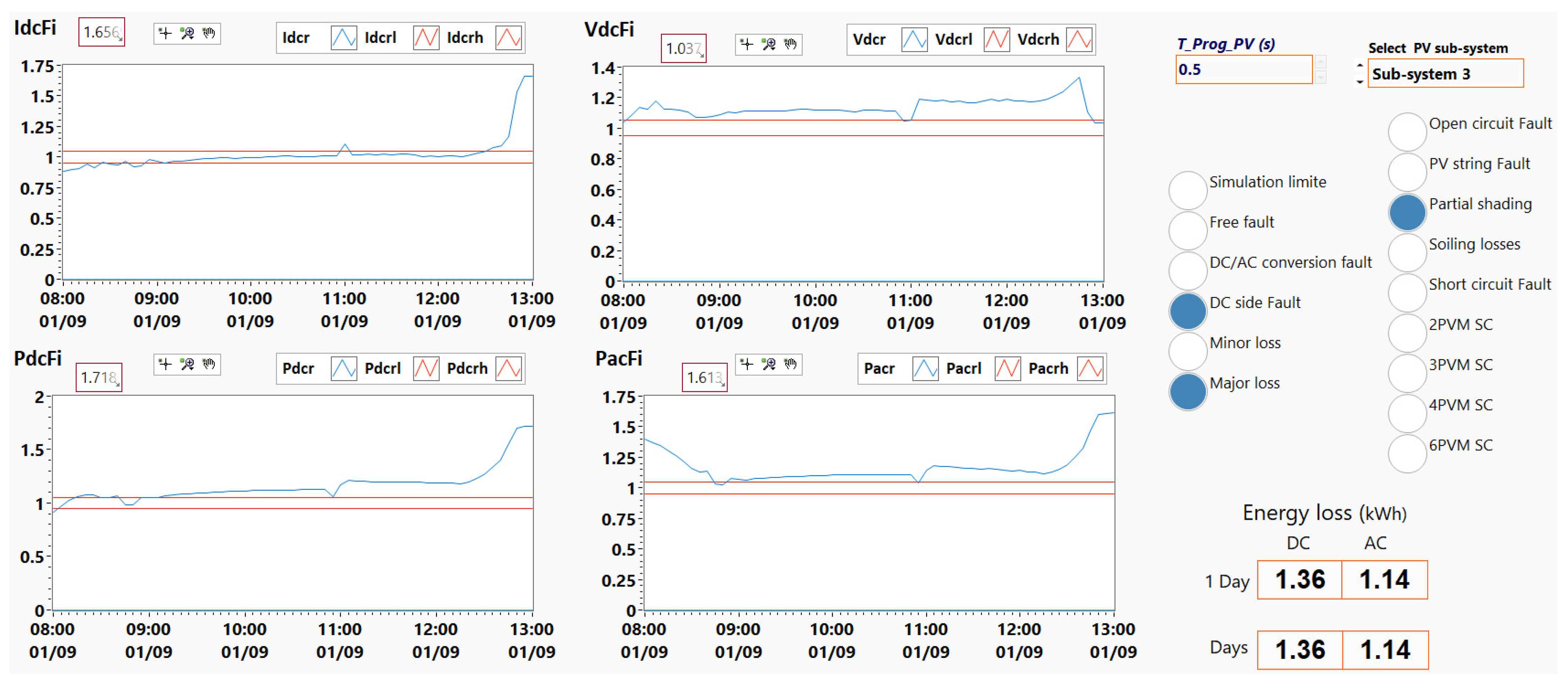
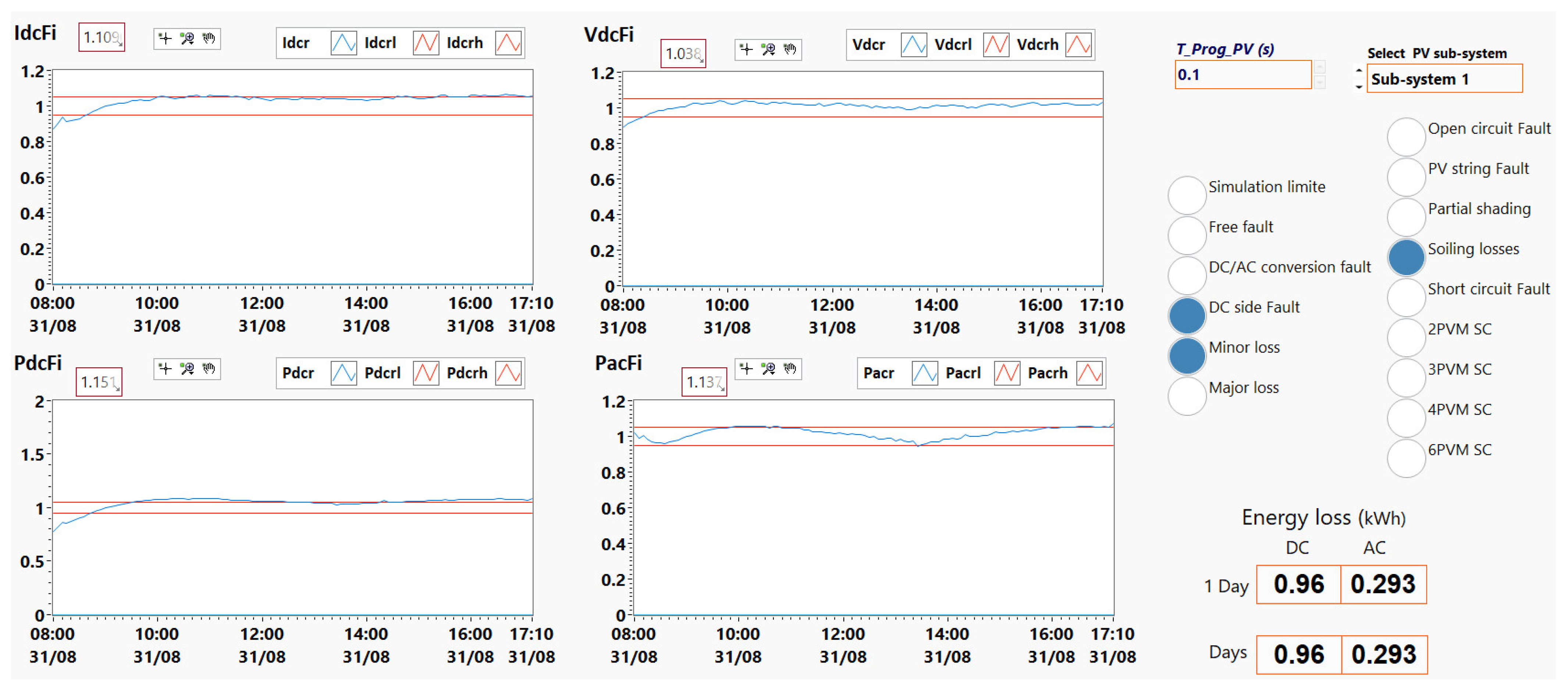
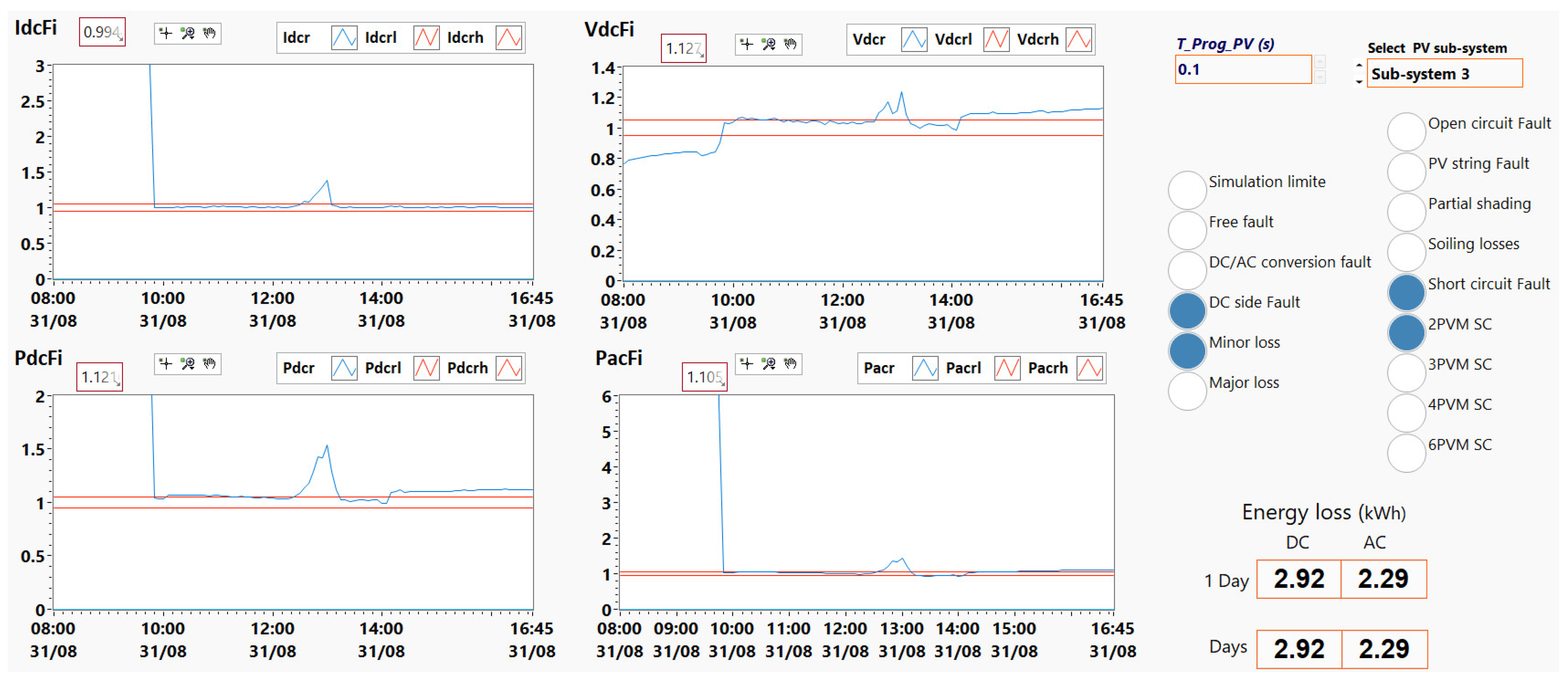
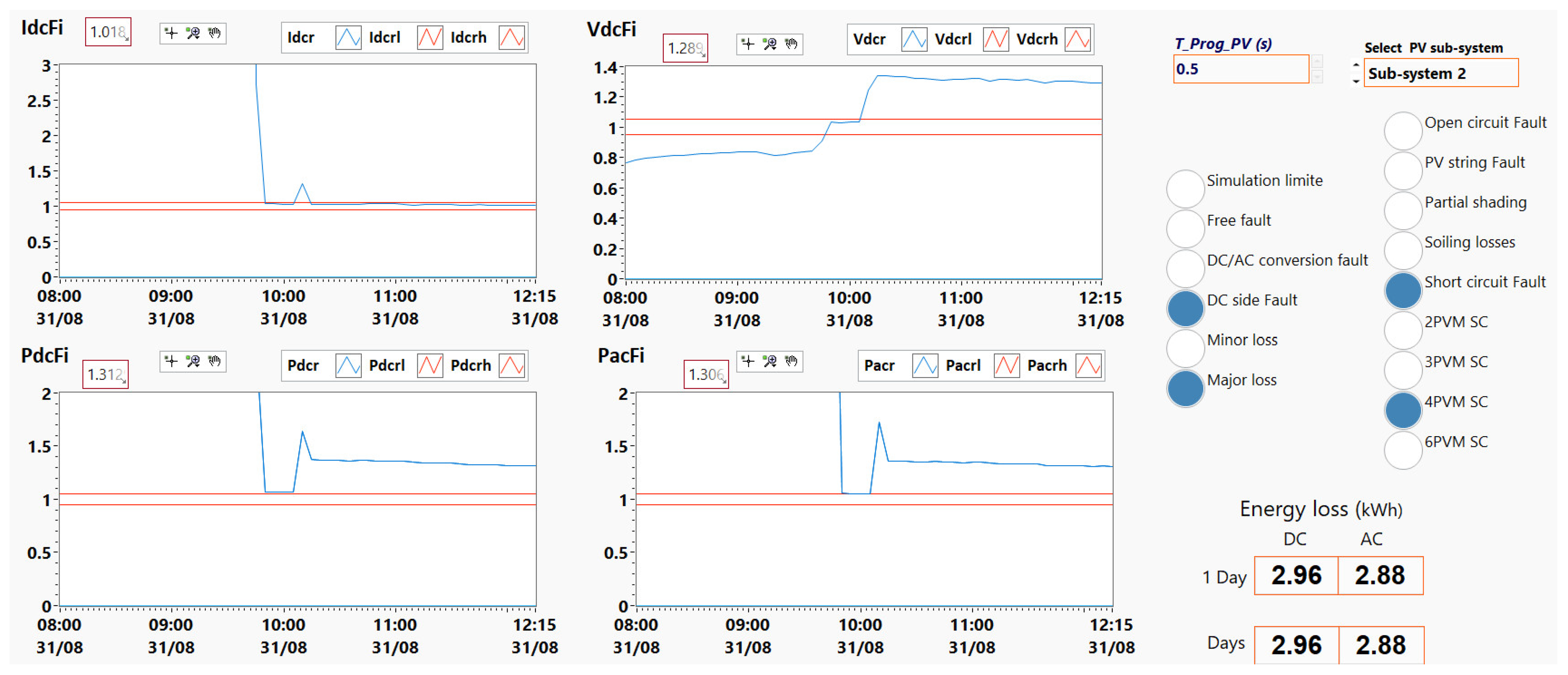
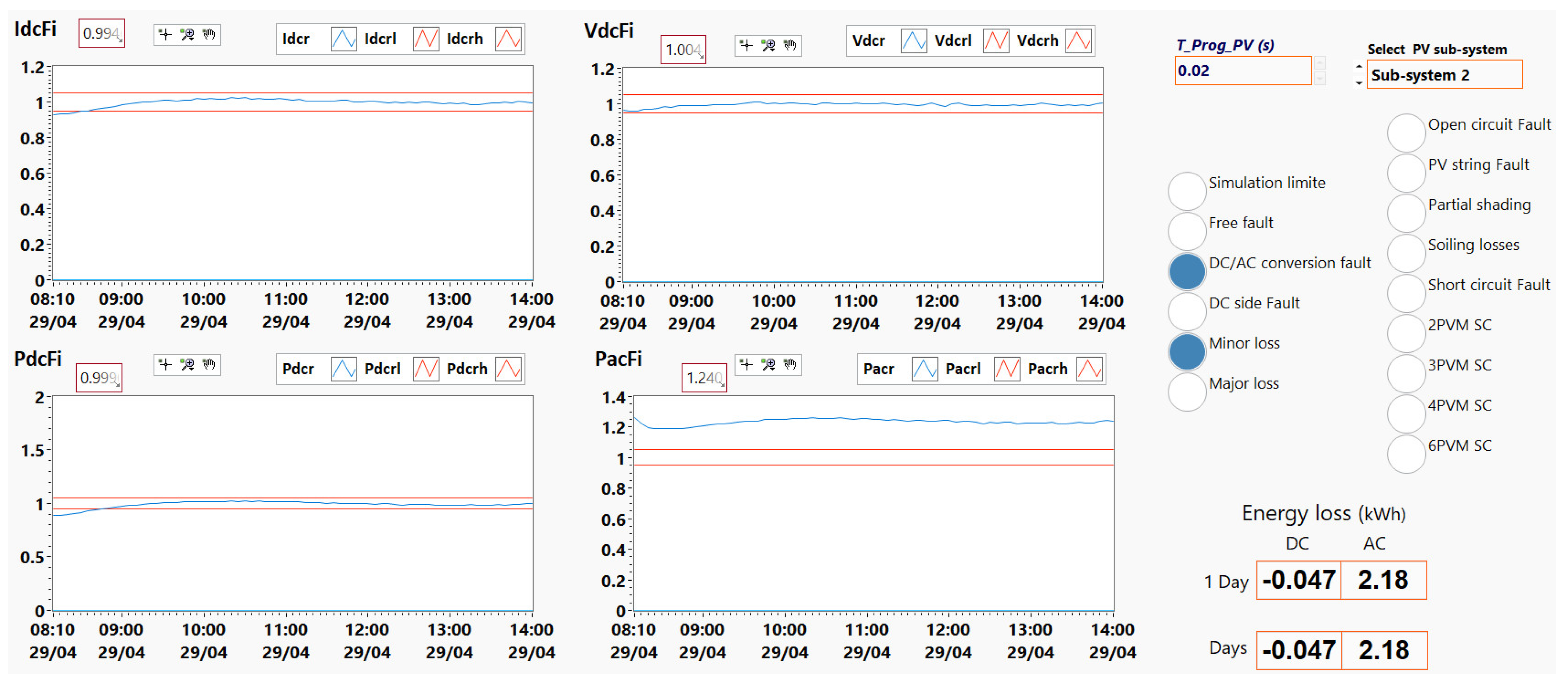
As shown in Figure 14, Figure 15, Figure 16, Figure 17 and Figure 18, the designed interface was very user-friendly and appealing, using modern indicators and waveform graphics. The modeling results were satisfactory, with a good fit to the reference electrical measurements for all PV subsystems. The considered models are easy to implement with low computational cost.

4. Fault Diagnosis of GCPVS Using PLR Method

4.1. Performance Loss Rate Method Using Four Electrical Indicators

In general, the FDD process is determined by comparing the normal data (i.e., the behavior predicted by simulation) and the faulty data for each type of fault (i.e., the behavior observed by measurement) [5].

Now, we propose a simple and reliable FDD technique under LabVIEW environment. Specifically, this technique utilizes the PLR evaluation of four indicators, namely (1) DC current indicator ($IdcR)$, (2) DC voltage indicator ($VdcR$), (3) DC power indicator ($PdcR$), and (4) AC power indicator ($PacR$). Here, the four indicators are calculated by dividing the simulated parameter over the measured parameter, as illustrated in Equations (15)–(18).

$$IdcR=\frac{Id{c}_{Sim}}{Id{c}_{Meas}}$$

(15)

$$VdcR=\frac{Vd{c}_{Sim}}{Vd{c}_{Meas}}$$

(16)

$$PdcR=\frac{Pd{c}_{Sim}}{Pd{c}_{Meas}}$$

(17)

$$PacR=\frac{Pa{c}_{Sim}}{Pa{c}_{Meas}}$$

(18)

The key aspect of the proposed method consists in its ability to uncover and identify different types of anomalies in DC and AC sides of a PV system. To detect anomalies and send alarms, two reference thresholds were added to each indicator, i.e., 1.05 for upper band and 0.95 for lower band.

For faults identification and localization, the assessment of the two power indicators $\left(\mathrm{i}.\mathrm{e}., PdcR \& PacR\right)$ makes it possible to localize the fault side either DC or AC. Since the majority of the malfunctions occur on the DC side, the refinement of the anomalies identification in the side DC is achieved using two other indicators ($\mathrm{i}.\mathrm{e}.,IdcR \& VdcR$). Each fault on the DC side has well-defined losses either in $IdcR$ or $VdcR$ or in both indicators at the same time. Based on this, the most probable fault can be identified. Figure 19 illustrates the flowchart of the developed strategy to uncover and identify the DC and AC anomalies affecting the GCPVS.

The four indicators were calculated under LabVIEW, several threshold limits were defined for each fault and anomalies in order to distinguish and identify each type. Figure 20 shows the Fault Detection and Identification (FDI) program via the Boolean function using graphical code under the LabVIEW environment.

After developing the graphical code under the LabVIEW environment for fault detection and identification, a new tab was added to the designed interface this tab contains the following features (Figure 21):

• ✓ DC and AC Energy loss indicators for 1 day and cumulated day
• ✓ Visual chart indicators (i.e., IdcFi, VdcFi, PdcFi, PacFi) with threshold limits
• ✓ Boolean digital indicators (LED) for fault type classification and identification.

4.2. Used Faults for Evaluation of the Proposed Method

The proposed technique was tested utilizing experimental data from a 9.54 kWp GCPVS at Algiers. Six kinds of anomalies were investigated in this study: (F1) Open circuit Fault (F2) PV string Fault, (F3) temporary partial shading, (F4) dust on the PV array, (F5) short circuit Fault with four (4) cases (i.e., 2, 3, 4, and 6 PV Modules short-circuited) and (F6) DC -AC conversion faults (Figure 22). Note that the electrical faults (i.e., F1, F2, and F5) were manually caused in numerous successive independent experiments. F3 and F4 were selected from the data recorded with these anomalies and. F6 was simulated with a DC/AC conversion efficiency of 80% instead of 96%.

4.2.1. Open Circuit Fault

This fault may appear if there is (1) an instantaneous disconnection of the inverter or the switching off of the residual current circuit breaker (RCCB).

The PV inverter disconnects if (1) the electrical characteristics of the output of the PV generator are outside the operating limit of the inverter or if there is (2) grid instability. This fault forces the shutdown of the PV installation till a new reconnection of the grid-tie inverter. If the residual currents (earth leakage) exceed 30 mA or if an electrical fault affects the PV plant, the RCCB switches off, provoking shutdown of the PV installation until it is manually switched on. Figure 23 illustrates the photos of the occurred open-circuit after the circuit breaker tripped or after the inverter’s temporary disconnection.

4.2.2. String Faults

Practically, PV string fault, which is a common fault, could cause large power losses in the affected PV installation. Usually, this malfunction occurs if (1) one of the DC protection components is damaged, (2) there is a bad cable contact with the terminal blocks, or 3) if there is a disconnection between the PV modules in series.

In this case, a string fault was generated by shutting down the PV string circuit breaker (Figure 24a) or by a real fault following an arc between the cable and the terminal block (Figure 24b).

4.2.3. Partial Shading

Another possible factor that can negatively affect the PV array performance is partial shading, which is defined as unequal distribution of solar irradiation on the PV array. Power losses due to shading could be caused by different types of obstacles (e.g., pylons, tall buildings, and trees) [7]. Here, as shown in Figure 25b the temporary partial shading on the PV array is caused by the shading formed by the two tall pylons (Figure 25a) during a period of the day. Figure 25b illustrates the pylon shadow on the PV subarray 3. In this section, the shading is therefore not modeled, it is considered an anomaly.

4.2.4. Soiling Losses

Soiling power losses are linked to several factors such as (1) environmental conditions, (2) frequency of rainfall, (3) tilt and type of PV module, (4) cleaning schedule, and others. Dust accumulation is one of the major problems with any solar PV system, especially in desert zones [69], it can negatively impact performance by causing power losses of up to 15% per year and possibly higher in sandstorm areas [14]. For the CGPVS in CDER, the power losses due to soiling are mainly caused by bird droppings and accumulated dust (Figure 26).

4.2.5. Short-Circuit Fault

Another common fault in PV systems consists of short-circuit faults that can occur in situations of incorrect wiring in PV modules. Whereas, the main sources of these faults are aging, vibration, and abrasion of PV modules [70]. This type of fault can degrade the performance or damage the PV module. Here, four short-circuit faults cases are considered (i.e., 2, 3, 4, and 6 short-circuited PV Modules) in order to evaluate the method based on electrical indicators rating. The faults are intentionally created by short-circuiting the modules in the same string according to the desired case. Figure 27 shows some cases of short circuit faults in the PV modules.

4.2.6. DC/AC Conversion Fault

PV Inverters convert energy from DC to AC with an efficiency that changes according to the inverter load. PV inverter manufacturers are usually able to provide the DC/AC efficiency profile for low, medium, and high voltages. The PV inverter may be affected by a drop in the desired efficiency according to the profile indicated in the datasheet following electrical problems or degradation of the DC/AC conversion components. This last fault was simulated with a DC/AC conversion efficiency of 80% instead of 96% which represents the rated efficiency of the inverter (i.e., Energy loss of around 16%).

4.3. Faults Detection and Identification Results

4.3.1. Open-Circuit Fault Detection

Let us now investigate the ability of the proposed method to identify an open circuit fault. The detection results illustrated in Figure 28 clearly shows that this fault can be recognized easily. For the open-circuit fault, the current indicator is equal to zero (i.e., no production Idc = 0) and the voltage indicator is less than 0.95 (i.e., the voltage is in open circuit Vdc = Voc).

4.3.2. PV String Fault Detection

This case aims to evaluate the ability of the developed technique to sense and locate PV string faults in a PV sub-array. In 9.54 kWp GCPVS, there are only two strings connected in parallel. In this case, the PV string fault causes a drop of around 50% of the rated power. The proposed method can easily discover this severe fault. To recognize this kind of fault, we examine the DC current and voltage indicators as depicted in Figure 29. We can see after the appearance of the string fault that the DC current is almost currency in two because we have two strings in parallel, while the DC voltage does not change significantly. From this analysis, we conclude that the occurred fault is due to string fault.

4.3.3. Partial Shading Detection

This experiment is devoted to assessing the ability of the PLR monitoring method to distinguish the temporary partial shading caused by pylons from other anomalies. To detect this fault, analysis of the dynamic behavior of both DC current and DC voltage indicators at the same time is essential. When a partial shading fault has occurred on the PV array, the DC current decreases according to the shading intensity and its distributed surface over the PV array, while the DC current is also linked to the series/parallel arrangement depending on shading, the second sign is the instability of DC voltage. So, to identify this fault, we use the combination of the two signs that appear. As we can see in Figure 30 the DC current indicator is well above the upper threshold (i.e., $IdcR$ = 1.65), up to this point, there is a possibility of three malfunctions (i.e., PV string fault, soiling losses, and partial shading), for the soiling losses the $IdcR$ is less than 1.2 and for string the $IdcR$ is around 2, then, there remains only one defect which is the partial shading. The parametric approach can identify the shading faults but there is a possibility of non-distinction with other faults on the DC side, which leads to false identification. The hybridization with other methods such as statistical, signal processing, and machine learning can give better precision and accuracy.

4.3.4. Soiling Losses Detection

In this scenario, we assess the performance of the proposed techniques in uncovering power losses caused by soiling chased by the accumulation of dust and bird droppings. From Figure 31 we can see that the detection based on the DC voltage indicator is in the confidence zone (i.e., 1.05 > $VdcR$ > 0.95), while DC current and DC power indicators are slightly above the upper threshold (i.e., $IdcR$ > 1.053 and $PdcR$ > 1.07), which means the existence of a small accumulation of dust which generates a minor power loss of around 1 kWh per day.

4.3.5. Short-Circuit Fault Detection

Let us now evaluate the potential of the presented technique to uncover and classify the level of short-circuit faults. For this, we present two cases: two and four short-circuited PV modules. The DC electrical parameters affected by this fault are mainly the DC voltage and the DC power. The DC current is not affected by this fault. Figure 32 illustrates the detection results for two short-circuited PV modules, we can see that the DC indicator gives no sign of fault (i.e., $IdcR$ = 0.996), while the DC voltage and DC power indicators are above the upper limit of 1.05. (i.e., $VdcR$ and $PdcR$ > 1.12), this situation corresponds to two short-circuited PV modules. This fault causes minor power losses. Note that recognizing a single module short circuit fault is a bit difficult.

Figure 33 illustrates the detection results of four short-circuited PV modules, we can see that the DC indicator gives no sign of fault (i.e., $IdcR$ = 1.01), while the DC voltage and DC power indicators are above the upper limit (i.e., $VdcR$ = 1.32 and $PdcR$ = 1.34). This situation corresponds to a voltage loss of four PV modules in series. This fault causes an important power loss.

4.3.6. DC/AC Efficiency Anomaly Detection

The final test evaluation is devoted to assessing the potential of the proposed technique to identify the fault on the AC side. In Figure 34 all DC Indicators are located between lower and upper thresholds limits, which means there are no malfunctions on the DC side, the AC power indicator is equal to 1.23, which largely exceeds the high threshold, which strongly indicates the presence of an inverter performance anomaly.

In summary, in this section, the nine faults’ cases were suitably identified and classified using a convivial user interface, along with other features that have been added to the interface. Indeed, this method can identify only two modules in a short circuit, on the other hand, the losses of one PV module among fifteen in series are a little hard to quantify. The distinction of partial shading from other faults is difficult because it has large ranges of variation in losses over time, the use of time-series monitoring or other signal processing techniques can provide a solution to this problem.

5. Conclusions

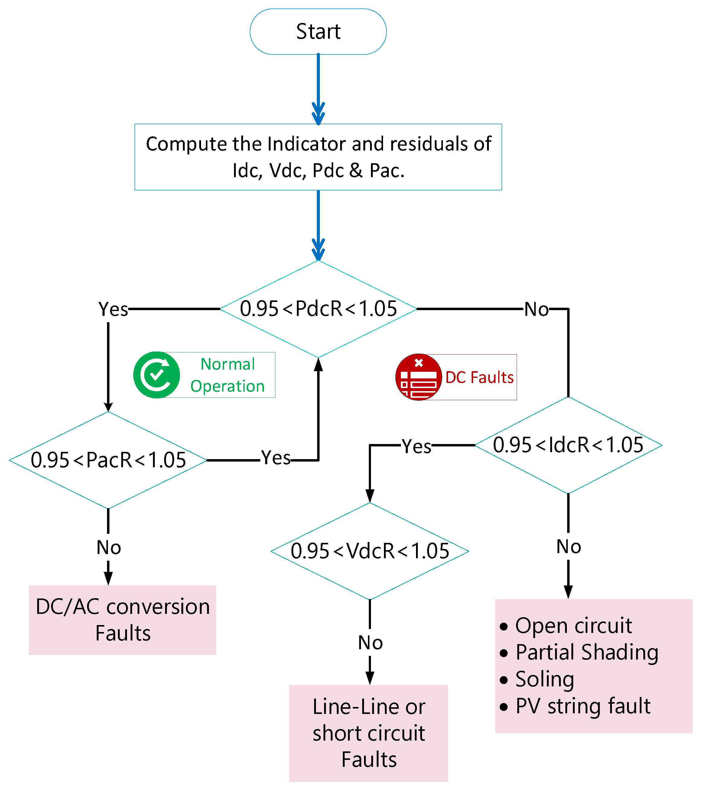
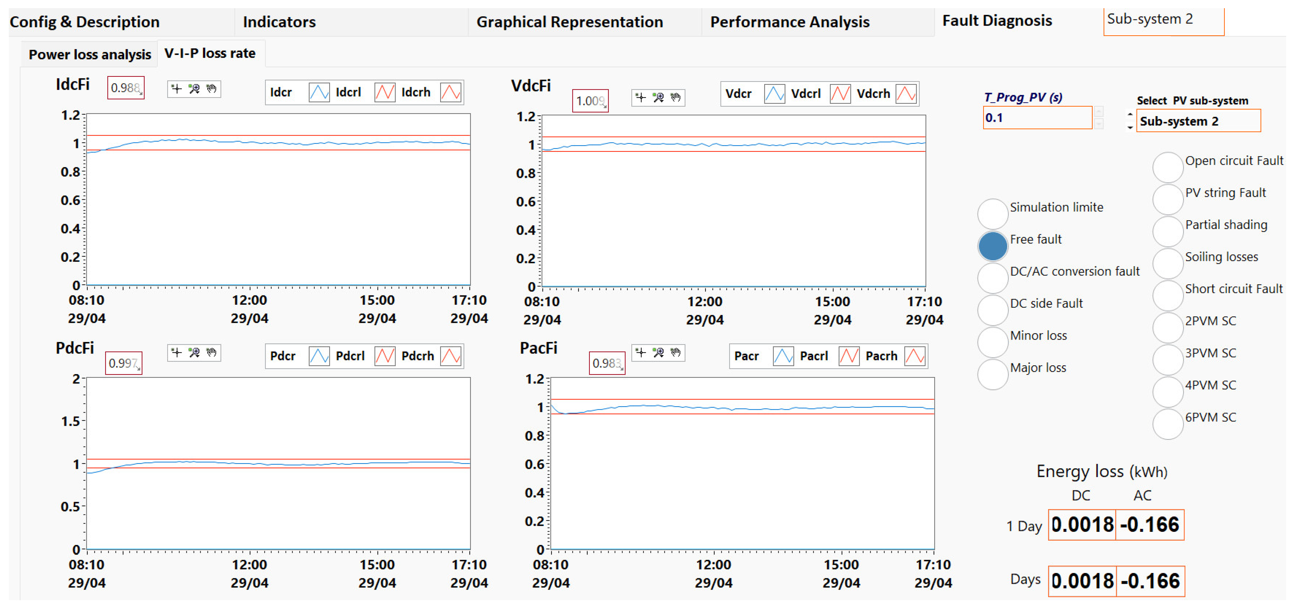
This paper introduces a simple and flexible diagnosis method under LabVIEW for detecting and identifying anomalies in a PV system. Toward this end, this method combines the desirable characteristics of empirical models and performance loss rate (PLR) evaluation. Specifically, the Sandia behavioral model of the PV array and the inverter were selected from several other models to accurately predict the electricity production and analyze the performance of the 9.54 kWp GCPVS. The results obtained from the Sandia models were validated and calibrated using reference experimental data in MATLAB. More specifically, the used models achieved good prediction quality in predicting DC current, DC power, and AC power with an $R^2$ of around 0.99, and an $R^2$ of about 0.98 for the PV cell temperature. On the other hand, for the predicted DC voltage of three subarrays, the $R^2$ is around 0.89. Overall, the prediction results were very satisfactory, with a better fit to the reference measured data. Here, the difference between the predicted and measured values are used for fault detection and diagnosis. The proposed fault detection and diagnosis technique is based on the PLR evaluation of four electrical indicators (i.e., DC current, DC voltage, DC power, and AC power) based on SANDIA parametric models. Importantly, four electrical indicators are used to further improve discrimination between the investigated anomalies in the DC and AC sides of the PV system. Results revealed that the proposed method can distinguish between faults under changeable climatic conditions and the nine faults’ cases were properly detected and identified using a convivial user interface, along with other features that were added to this interface. Essentially, the proposed technique is not complex and easy to integrate into the real-time monitoring program. This study revealed the promising performance of the combined empirical models with the PLR approach for anomaly detection and identification in PV systems.

Despite the improved detection performance, partial shading is not obvious to discriminate from other faults on the DC side, which can lead to false identification. Thus, future works will improve its capacity to discriminate partial shading by intelligent signal processing of a shading anomaly. Moreover, we plan to evaluate the performance loss rate [44] with advanced machine learning and deep learning models [71]. Furthermore, another direction of improvement consists of adding Internet of Things (IoT) functionalities [72] to the monitoring system, which improves the online supervision of performance analysis and malfunctions alarms in real-time [73].