Abstract
In recent decades, the traditional monopolistic energy exchange market has been replaced by deregulated, competitive marketplaces in which electricity may be purchased and sold at market prices like any other commodity. As a result, the deregulation of the electricity industry has produced a demand for wholesale organized marketplaces. Price predictions, which are primarily meant to establish the market clearing price, have become a significant factor to an energy company’s decision making and strategic development. Recently, the fast development of deep learning algorithms, as well as the deployment of front-end metaheuristic optimization approaches, have resulted in the efficient development of enhanced prediction models that are used for electricity price forecasting. In this paper, the development of six highly accurate, robust and optimized data-driven forecasting models in conjunction with an optimized Variational Mode Decomposition method and the K-Means clustering algorithm for short-term electricity price forecasting is proposed. In this work, we also establish an Inverted and Discrete Particle Swarm Optimization approach that is implemented for the optimization of the Variational Mode Decomposition method. The prediction of the day-ahead electricity prices is based on historical weather and price data of the deregulated Greek electricity market. The resulting forecasting outcomes are thoroughly compared in order to address which of the two proposed divide-and-conquer preprocessing approaches results in more accuracy concerning the issue of short-term electricity price forecasting. Finally, the proposed technique that produces the smallest error in the electricity price forecasting is based on Variational Mode Decomposition, which is optimized through the proposed variation of Particle Swarm Optimization, with a mean absolute percentage error value of 6.15%.
1. Introduction
The landscape of the formerly monopolistic power systems has changed over the past few decades as a result of deregulation and the introduction of competitive markets [1]. In many countries worldwide, electricity is traded through spot and derivative contracts in accordance with strict market principles [2]. Electricity, on the other hand, is economically unstorable and contradicts the fundamental operating principle of power systems, which calls for a permanent equilibrium between production and consumption. With the advent of restructuring in the electric power industry, the price of electricity has become the focal point of all power market activity. The price of electricity is the most significant signal to all market players in a power market and the market-clearing price is the most fundamental pricing notion [3]. Following the receipt of bids, the Independent System Operator (ISO) combines the supply bids into a supply curve and the demand bids into a demand curve. The market-clearing price is determined at the point where these two curves intersect and identifying it is essential for the efficient and orderly operation of power systems [4].
Electricity price forecasting can be divided into three categories based on length of time: short-term, mid-term and long-term. In order to set up bilateral transactions or define bidding strategies on the spot market, this study primarily focuses on developing data-driven models for predicting short-term electricity prices. The spot electricity market usually conducts day-ahead auctions and does not support uninterrupted trade. Agents are required to submit their bids and offers for the delivery of electricity during each hour of the following day before a specific market closing time on the previous day.
In comparison to the load forecasting problem [5], where the load curve is mostly homogenous and its variations are cyclic [6], the electricity price forecasting problem has a non-homogeneous pricing curve and only weakly cyclic variations [7]. At the same time, price spikes that occur when a system’s load level approaches its generating capacity limit have an explicit impact on prediction accuracy [8,9,10]. Although the price of power is highly volatile [11], it is not considered random. It is obvious that various physical factors could influence the electricity price, with some variables dominating over others. As a result, in short-term applications, it is critical to identify the parameters that have the most impact on price predictions. The time, i.e., the hour of the day, day of the week, etc., special days, previous pricing values and historical and predicted load values are the parameters that have the greatest influence on the outcome of electricity price forecasting.
Short-term electricity forecasting can be approached using two strategies, statistical methods [12] and computational intelligence models [13]. Statistical approaches forecast the current price by combining previous prices with prior or present values of exogenous factors. Simple Moving Average, Exponential Smoothing and Autoregressive Integration Moving Average (ARIMA) are some statical strategies that are successfully implemented in electricity price forecasting [14,15,16]. Due to their flexibility and ability to manage complexity and non-linearity, computational intelligence approaches have been created to solve problems that traditional statical methods are inefficient at handling [17]. Artificial Neural Networks (ANNs), Fuzzy Systems, Support Vector Machines (SVM), techniques for evolutionary computation and hybrid approaches that combine two or more computational intelligence algorithms have yielded satisfactory price prediction results.
The majority of recent papers in the literature that address the problem of predicting electricity prices usually propose a regressor model, an optimization method and an algorithm for signal decomposition of the price. Unlike the few regression models used to predict the price of electricity, the literature is replete with optimization strategies. Support Vector Regression (SVR) models, ANNs and Extreme Learning Machines (ELMs) are the major price forecasting models. Empirical Mode Decomposition (EMD), either as is or in some modified form, and Variational Mode Decomposition (VMD) are the primary techniques employed for signal decomposition. Those two approaches have found extensive application in the existing literature on price forecasting in general and their results have been thoroughly compared [18].
In [19], Ribeiro et al. use a combination of several non-linear models, including ELMs, Gradient Boosting Machine (GBM), SVR models and Gaussian Process (GP), to predict commercial and industrial electricity prices in Brazil for one to three months ahead. The suggested model is based on exogenous factors such as power supply, lagging pricing and electricity demand and the hyperparameters are chosen using the Complementary Ensemble Empirical Mode Decomposition (CEEMD) technique, the fine tuning of which is based on the implementation of the Coyote Optimization Algorithm (COA). Similarly, Qiu et al. [20] used EMD to decompose the electricity price signal into numerous Intrinsic Mode Functions (IMFs) and a Kernel Ridge Regression (KRR) model to predict each IMF’s trends. The predictions of all IMFs were then utilized by an SVR to provide the aggregated price forecasting result for the Australian Energy Market Operator. Although this proposed method improved accuracy and efficiency compared to traditional methods, it failed to produce satisfactory mean absolute percentage error (MAPE) values. In another study [21], Ensemble Empirical Mode Decomposition was used in conjunction with various regression models such as Recurrent Neural Network (RNN), Multi-Layer Perceptron (MLP), SVR and ELM to obtain the actual predicted price of electricity based on data from the power systems of New South Wales (NSW), Queensland (QLD) and Victoria (VIC). According to the findings of this study, computational intelligence models produce a large MAPE; however, the suggested ELM model paired with the Ensemble Empirical Mode Decomposition manages to reduce the MAPE to less than 10%.
Unlike EMD, VMD has not been widely adopted in the literature on electrical price forecasting, but it is found in applications for forecasting challenges such as carbon price prediction [22], crude oil price forecasting [23] and short-term wind power projection [24]. In [25], Yang et al. offer an adaptive hybrid forecasting model employing an Improved Multi-Objective Sine Cosine algorithm (IMOSCA) for the optimization of a Regularized Extreme Learning Machine (RELM), which is the first attempt to deal with EPF based on Variational Mode Decomposition. The MAPE values are close to 6% when using the proposed model. In a similar effort, Wang et al. [26] used the Improved Variational Mode Decomposition (IVMD), as a data preprocessing technique, in order to decompose the original electricity price series into several modes. Then, they utilize the Chaotic Sine Cosine Algorithm (CSCA) enhanced with the Phase Space Reconstruction (PSR) in order to select the optimal input vector of each mode and use it for the prediction of the electricity price based on an Outlier-Robust Extreme Learning Machine (ORELM) model.
Similarly, clustering is another ensembled preprocessing method utilized to improve the outcomes of electricity price predictions. Although the theoretical foundations of these two preprocessing approaches differ, they both operate on the divide-and-conquer concept. A divide-and-conquer algorithm recursively divides a problem into two or more sub-problems of the same or related nature, until they are simple enough to resolve directly. The sub-problems’ answers are then merged to provide a solution to the initial problem. As a result, the signal decomposition method may be safely termed a clustering method.
An initial implementation of the clustering approach is conducted in [27], where Ghayekhloo et al. present an enhanced data clustering technique for price-load input data in order to group them into an appropriate number of subsets utilizing six new game-theoretic methods. This unique cluster selection method based on the persistence approach is used to identify the best suitable cluster as the input to a Bayesian Recurrent Neural Network (BRNN) for electricity market day-ahead price forecasting. The proposed forecast model surpasses current state-of-the-art forecasting algorithms, demonstrating a significant improvement in prediction accuracy. In a different approach to data clustering, Pourhaji et al. [28] investigate the seasonal data clustering effect on price forecasting. The energy price forecasting for the day-ahead horizon is based on data from Ontario province in Canada. The important parameters of the prediction are identified using the Gray Correlation Analysis (GCA) approach and the day-ahead electricity price forecasting is achieved using a Long Short-Term Memory (LSTM) model. Finally, the predictions are compared in three modes: non-clustering, seasonal clustering and monthly clustering. In an alternative study, Wang et al. [29] propose a classification modeling strategy for predicting electricity prices based on daily pattern prediction (DPP). In this study, K-Means is used to cluster all of the historical daily electricity price curves and then the suggested DPP model is used to detect the following day’s pricing trend from the forecasting data supplied by numerous traditional forecasting methods. Then, for each individual daily pattern, a classification predicting model is developed and a credibility check on the DPP result determines which of them will be eventually employed. This approach is applied to real electricity price data from the PJM market, yielding more accurate forecasting results than the single integrated modeling approaches.
This paper examines the issue of short-term electricity price forecasting using historical price data from the Greek electricity market. More specifically, six robust prediction models that use subsets of the original dataset resulting from the application of VMD and the K-Means clustering algorithm are proposed. The regressor approaches used are an SVM, an MLP neural network and an XGBoost model, whose optimization is based on the Base Optimizing Algorithm (BOA). The forecasting results provided by each model are compared to each other, based on the MAPE, with the aim of choosing the forecasting model that provides the most accuracy. More specifically, by extensively studying the existing literature and identifying some gaps, the fundamental aspiration of this paper is:
- To develop robust and optimized data-driven forecasting models in conjunction with the VMD or the K-Means algorithm that will improve the accuracy of electricity price predictions, compared to the existing results;
- To propose an enhanced modification of the Particle Swarm Optimization (PSO) technique used for the selection of the discrete values of the VMD algorithms’ hyperparameters. The proposed algorithm is applied in identifying the local maximum (and not the local minimum as usual) of a well-defined objective function;
- To propose the use of BOA as a front-end metaheuristic algorithm that will determine the appropriate values of the hyperparameters of each regression model;
- To propose an XGBoost prediction model that will produce accurate results in a short convergence time;
- To be the first paper that compares the effect of the signal decomposition and clustering approach on the results of electricity price forecasting.
This paper is organized as follows. Section 2 analyzes the materials and methods used for the establishment of the proposed robust and optimized data-driven forecasting models. In Section 3, the numerical results from the implementation of the proposed approaches in short-term electricity price forecasting based on historical data of the Greek electricity market are presented. In Section 4, those results are analyzed and compared in order to determine the performance of the preprocessing techniques in terms of price prediction accuracy. Section 5 summarizes and concludes the results of the proposed work and suggests topics for further research in the area of short-term electricity price forecasting.
2. Materials and Methods
In this section, the algorithmic structures of the signal decomposition methods, the K-Means clustering technique, the Base Optimizing Algorithm, as well as the various regression models used to design robust, highly accurate and data-driven forecasting approaches are presented and analyzed.
2.1. Signal Decomposition
Electricity price forecasting is mainly based on the signal that reflects the price of electricity to a currency (EUR/MWh or USD/MWh). This signal has certain oddities because it is influenced by many exogenous sources, yet it has a distinctive curve in the domain of time. Therefore, a variety of signal decomposition techniques can be used to better comprehend and monitor the signal relating to the price of electricity. According to the theory of decomposition, every signal is made up of various intrinsic oscillation modes. Each mode is an oscillation, or Intrinsic Mode Function (IMF), that is symmetric with respect to the local mean and has a maximum difference of one in the number of local extrema and zero-crossings.
A first approach to signal decomposition was presented by Huang et al. by establishing the Empirical Mode Decomposition (EMD) technique [30]. EMD is an entirely data-driven strategy that decomposes a signal into several modes of unidentified but distinct spectral bands [31]. One of EMD’s key advantages is that it automatically determines the ideal number of modes based on the signal’s characteristics. The derived modes are hierarchically arranged so that the first IMF has the highest-frequency component and the residual signal is left with the information of lower-frequency components [32]. On the other hand, the algorithm’s robustness of decomposition is diminished by the absence of mathematical theory. Due to its recursive execution, EMD is noted for having restrictions including susceptibility to noise and sampling [33] and does not support backward error correction. Additionally, it is prone to undermining the accurate identification of the extrema and as a result of that, of their upper and lower envelopes [34]. This is due to the phenomenon of over-decomposition of a signal, which occurs when more IMFs are extracted than the number of oscillatory modes that comprise the original signal.
More robust variants, including Ensemble Empirical Mode Decomposition (EEMD) [35] and Complete Ensemble Empirical Mode Decomposition with Adaptive Noise (CEEMDAN) [36], have recently been proposed to solve the original EMD algorithm’s shortcomings in terms of sensitivity to noise and sampling. EEMD is a noise-assisted data analysis technique that may spontaneously divide the original signal into IMFs without the need of predetermined, subjective criteria. CEEMDAN is a variation of the EEMD algorithm, which offers a precise reconstruction of the original signal and improved IMF spectral separation. Even though it requires more computational power, this enhanced version, which uses White Gaussian Noise, is intended to significantly lessen the negative impacts of noise.
In a later attempt, Dragomiretskiy and Zosso [37] proposed VMD, a more reliable and mathematically solid method. This method has been widely used in the diagnosis of gearbox faults [38], the fault diagnosis scheme for rolling bearings [39], the seismic time-frequency analysis [40], the forecasting of crude oil prices [41], the prediction of wind power [42] and the forecasting of short-term load [43]. In order to create a reliable, robust and accurate forecast model that might be employed in the EPF, this paper focuses on the application of VMD in the signal that reflects the hourly price of electricity. Therefore, the VMD algorithm’s structure as well as its benefits over competing decomposition techniques should be taken into account. The purpose of VMD is to decompose an input signal with real value into a discrete number of IMFs that are compact around a central pulsation, which is to be identified simultaneously with the decomposition. In particular, the squared norm of each IMF’s Hilbert supplemented analytic signal [32] is used to determine each IMF’s bandwidth. Mixing each mode with a tuned exponential function causes the spectrum of each mode to be displaced on the approximated angular frequency. The demodulated signal’s Gaussian smoothness, which is the gradient’s squared Euclidean norm (L2-norm), is ultimately used to determine the bandwidth. The IMFs are updated using straightforward Wiener filtering in the Fourier domain to address the variational problem.
The VMD technique is resilient to noise and has been widely employed because it has been proven to be sensitive in identifying weak side-band signals that are frequently covered up by background noise [44]. As a result, it has been asserted that the VMD technique is effective for signal denoising and detrended fluctuation analysis, with a temporal complexity order comparable to that of EMD [45]. The decomposed modes are extracted continuously rather than iteratively grading enhanced error balancing, which makes EMD non-recursive [46]. It has also been suggested in real-time pattern recognition implementations, demonstrating a significant improvement in efficiency over EMD and wavelet-based methods [47].
The VMD algorithm is parameter sensitive, according to [37], as the decomposition outcome mainly depends on the choice of penalty constant and decomposition number K. Each IMF component has a constrained bandwidth under specifics and K. The requirement to predefine in how many modes (or clusters) data are to be binned is a common weakness of many segmentation methods. The parameter K in the VMD process determines how many modes the original signal is dived into. The selection of the penalty parameter determines the IMFs’ bandwidth size. Therefore, the ideal pairing of parameters K and should be chosen in order to prevent overdecomposition/underdecomposition of the provided signal. These parameters are chosen either empirically, through a process of trial and error, or with an optimization algorithm. Particle Swarm Optimization (PSO) [48], Cuckoo Search (CS) [49], Gray Wolf Optimizer [50] and the Chaotic Sine Cosine (CSC) method [51] are a few optimization techniques that are utilized to configure VMD appropriately. Inverted and Discrete Particle Swarm Optimization (IDPSO), a novel and reliable methodology, is used in this study as the foundation for VMD parameterization. A mathematical and algorithmic analysis of IDPSO is provided in the following section.
Inverted and Discrete Particle Swarm Optimization into Variational Mode Decomposition
Particle Swarm Optimization (PSO) is a bio-inspired algorithm that has been widely employed in deep learning situations to optimize continuous nonlinear functions [52]. This heuristic approach aims to locate the best solution in a high-dimensional space, or as close to it as is possible [53,54]. PSO differs from other optimization techniques since it does not depend on the gradient or any differential form of the objective function in order to arrive at a solution that is near the global minimum [55]. Since the PSO is used to minimize an objective function for certain pairs of (K, ) parameters in order to produce the best practicable parametrization, it may be simply adapted to the selection of these parameters in the VMD approach. The formulation of an objective function should be taken into account initially because the VMD technique does not include any mathematical functions that should be minimized. Due to this, different versions of multiple objective functions have been presented in the literature, including the ratio of 1 to kurtosis of decomposed signals [56], the average of the envelope and Renyi entropy of modes [57] and the ratio of the mean to variation of the cross-correlation signal between the original signal and the IMFs [39]. In this paper, the objective function used is that of [39] and therefore its mathematical function should be rendered.
Cross-correlation is a metric used in signal processing to determine how similar two signals are to each other. Correlation of two signals is defined as the convolution of one signal with the functionally inverse representation of the other signal. The cross-correlation of the two input signals is the name given to the resulting signal. The cross-correlation signal’s amplitude serves as an indicator of how closely the received signal resembles the target signal [58]. The mathematical expression for the cross-correlation of continuous time signals and is given by Equation (1):
Cross-correlation is used as a measure of the correlation between the initial signal and the decomposed modes as a result of the application of VMD for particular pairs K and in terms of the decomposition of the price signal. Cross-correlation, however, cannot be an objective function in itself; hence, it is important to use the information that indicates how much the cross-correlation signal varies from the mean value. The cross-correlation signal between the original signal and all IMFs’ mean values and their variance is therefore used to establish the proposed objective function. The objective function used in the proposed, enhanced version of PSO is given in Equation (2):
Equation (3) attributes the variance of the cross-correlation signal between the original signal and the decomposed modes:
where N is the number of samples, is the value of the signal at the i-th sample and is the mean of the signal. Therefore, the appropriate parameterization of the VMD is given for the constants K and in which greater correlation results between the original signal and all IMFs. Therefore, the pair (K, ) that maximizes the objective function of Equation (2) must be found.
Once the proper objective function has been established to be employed by the PSO in order to acquire the correct decomposition of the signal of the electricity price, the need for the application of an appropriate variation of this heuristic algorithm can be easily identified. The development of an inverted version of PSO is initially required, where it will search for the global maximum of the objective function rather than its global minimum. The implementation of PSO in discrete values of K and should also be considered for this specific differentiation, as demanded by the algorithmic analysis of VMD. This paper proposes the establishment of an Inverted and Discrete Particle Swarm Optimization (IDPSO) algorithm that will be applied as a front-end heuristic algorithm for the optimal parameterization of the VMD algorithm. The novel IDPSO-VMD algorithm is analyzed as follows:
- Step 1: Initialize the values K and within the defined solution space. The pair (K, ) is a group of particles, the number of which is defined by the user, that is initialized with random values in order to find the global maximum of the objective function;
- Step 2: For the initial particles of Step 1 the VMD algorithm is executed and the values of the objective function are calculated;
- Step 3: The solution of the algorithm is considered to be the largest value of the objective function found in Step 2;
- Step 5: For the new particles, the VMD algorithm is executed and the values of the objective function are calculated;
- Step 6: In cases where the objective function displays a higher value of the existing global best solution for the new particles, the optimal solution is updated;
- Step 7: Steps 4–6 are repeated until the parameters K and stop being updated, i.e., the particles stop moving towards the point that shows the optimal solution or the algorithm for the maximum number of repetitions set by the user is reached;
- Step 8: The algorithm returns the best possible solution.
In Equations (4) and (6) the parameters w, and are user-defined constants that represent the inertia of the particles and how sensitive they are to the current best and the global best solution, respectively. The variables denoted as and are random numbers between 0 and 1. Therefore, the results of Equations (4) and (6) become a distinct value when applying a well-defined Python function, which returns the closest to the resultant integer number.
2.2. Data Clustering
Unsupervised learning techniques like clustering are frequently used to discover significant structure, explanatory underlying processes and generative features in a large dataset. The fundamental concept behind clustering is that homogeneous data groups are produced by splitting a given set of data points into a set of groups that are as identical as possible. It is crucial because it establishes the inherent grouping among the existing unlabeled data. Because the efficiency of clustering is directly affected by the type of data, it is not surprising that a variety of methodologies, including probabilistic, distance-based, spectral and density-based strategies, are utilized in the clustering process. Each of these techniques has advantages and limitations of its own and may be effective in various situations and different domains.
Clustering analysis is widely utilized in a variety of fields, including market research, pattern recognition, image processing and the analysis of biological data. In recent years, the necessity to upgrade traditional power systems and convert them to Smart Grids has expanded the number of installed smart meters, which has increased the amount of electrical network data that is currently available. Therefore, clustering finds wide application in datasets that consist of time-series concerning both load forecasting and electricity price forecasting. It should be highlighted that identifying data that are developing over time differs significantly from classifying data that are static. Due to the significant differences in the behavior of the data variables across different parts of the datasets, high dimensional datasets, such as those referring to short-term electricity price forecasting, provide unique difficulties for cluster analysis.
Time series clustering frequently involves the use of conventional cluster analysis techniques including hierarchical and non-hierarchical clustering approaches. In this first case, an appropriate distance measure for comparing time series is established, inheriting the dynamic aspects of the time series and then a typical hierarchical cluster analysis is used while utilizing the provided distance measure. In the latter case, partitioning clustering approaches divide a set of data points into K clusters. This procedure typically follows the optimization of a criterion function that represents the inner variability of the clusters during the minimization of an objective function. One of the most well-known and often used non-hierarchical clustering algorithms is K-Means clustering, which aims to partition the data in an effective manner by minimizing the Sum of Squared Errors (SSE) criterion through an iterative optimization process. Denoting as the k-th cluster, a point in , is the mean (centroid) of the k-th cluster and K the number of clusters, the SSE is given by Equation (8):
K-Means starts by choosing K representative points as the initial centroids. Next, based typically on Euclidian distance, each point is allocated to the nearest centroid. The centroids for each cluster are updated after the clusters have formed. Afterwards, the algorithm iteratively repeats these two steps until the centroids remain the same or a different relaxed convergence condition is satisfied. The initial centroids and the estimated K-Means optimal number of clusters are the two main variables that can affect the performance of the method. The most important aspects influencing the efficiency of the K-Means algorithm are the initial centroids and estimating the ideal number of clusters K.
The initial centroids in this study are chosen using the K-Means++ approach. This algorithm employs a straightforward probability-based approach in which the first centroid is chosen at random. The next centroid determined is the one that is farthest away from the present centroid. This decision is based on a weighted probability score. The selection process is repeated for K iterations. The Elbow Method is used to solve the problem of estimating the ideal number of clusters K.
Determining the Optimal Number of Clusters—Elbow Method
A major challenge in partitioning clustering is determining the optimal number of clusters in a dataset, which involves the user defining the number of clusters K to be formed. The appropriate number of clusters is rather subjective and depends on the method used to measure similarities as well as the clustering algorithm’s parameters. As previously stated, the purpose of the K-Means clustering algorithm is to segment data effectively while minimizing SSE. However, its rate of decrease varies depending on whether it is above or below the optimal number of clusters K. The inertia reduces rapidly for , whereas it decreases slowly for . The user can therefore identify the point where the curve bends or elbows and determine this point as the ideal number of clusters by visualizing the inertia across a range of k. However, because various users may locate the elbow in a different spot, this method is somewhat arbitrary.
In our work, the clustering algorithm under consideration is K-Means and its implementation is based on Python’s library scikit-learn [59]. The clustering approach is implemented on historical data of electricity price and hourly weather data such as temperature and humidity. The ideal number of clusters is determined using the Elbow Method. Therefore, for a range of clusters, the SSE resulting from the use of the K-Means algorithm is calculated and graphed.
2.3. Regression Models
In this paper, the use of an SVR, an MLP neural network as well as the innovative and highly efficient XGBoost model is proposed to address the electricity price forecasting issue. The SVR and the MLP neural network were built based on the scikit-learn library [59], and the XGBoost model with the corresponding Python library.
2.3.1. Support Vector Machines
Support Vector Machine is an algorithmic approach appropriate for supervised learning, the primary intention of which is to find a hyperplane in an N-dimensional space (where N is the number of features) that distinctly allocates the data points [60]. There is a variety of different hyperplanes that might be used to split the subclasses of data points. The primary goal of using SVMs to address a classification problem is to determine a hyperplane that has the maximum margin, or the maximum distance between data points from the distinct classes. When applied to a regression problem, they aim to predict a real function (f) using pairs of input—output training data produced similarly and independently dispersed in accordance with an unknown probability distribution function. Since Support Vector Regression (SVR) is one of the regression models employed in the problem of short-term electricity price forecasting, its method will be investigated in this study.
Margin is a classification-specific concept. The purpose of SVR is to establish a function that has the least amount of deviation () from the real targets for all of the training data while also being as flat as possible in order to avoid using overcomplicated regression functions. Thus, results with inaccuracy less than are accepted, but deviations greater than are unacceptable [61]. Using the -sensitive loss function of Equation (9), an equivalent of the margin is built in the space of the target values y:
A regression function that generalizes efficiently is determined by modifying both the regression ability via the weight vector w and the loss function. The data are fitted to a tube with a radius . The trade-off between the complexity term and the empirical error is adjusted by the regularization constant C, which accepts values greater than zero [61]. The objective function of Equation (10) that should be minimized, known as C-SVR, is as follows:
SVRs are extensively used in short-term electricity price forecasting applications because of their many advantages, the most important of which are encapsulated in their robustness to outliers, their ease of implementation, which reduces their computational complexity and their ability to use a symmetrical loss function, which equally penalizes high and low misestimates [62]. Therefore, SVRs should be optimized by selecting the proper hyperparameters in order to be implemented effectively. The parameters that should be optimized using the BOA metaheuristic algorithm are the kernel type, the strictly positive regularization parameter C and the radius of the epsilon tube-SVR model [63].
2.3.2. Extreme Gradient Boosting
A gradient boosting framework is used by the decision-tree-based ensemble machine learning method known as Extreme Gradient Boosting (XGBoost) [64]. Boosting is an ensemble strategy in which new models are sequentially introduced to rectify errors committed by previous models until no more improvements are possible [65]. Gradient boosting is a method where new models are made to forecast the errors or residuals of earlier models, which are then combined together to provide the final prediction. Because it employs a gradient descent approach to reduce loss when introducing new models, it is known as gradient boosting [66]. The mathematical aspect of the XGBoost algorithm, which explains how boosting is accomplished, and the algorithm’s greedy behavior are fully discussed in [64].
XGBoost is a novel sparsity-aware parallel tree learning algorithm built on a highly scalable end-to-end tree boosting framework. This algorithm has piqued the scientific community’s interest because it focuses on computational speed and model performance. It is a perfect combination of software and hardware optimization techniques as it produces superior results with fewer computing resources in the shortest amount of time.
To properly leverage the benefits of the XGBoost method in our work, the model needs to be fine tuned with the suitable selection of specific hyperparameters. As previously stated, the BOA method is used to determine the learning rate, i.e., a step size shrinkage used to prevent overfitting, the parameter, which is a minimum loss reduction required to make a further partition on a tree’s leaf node, the maximum depth of a tree and the regularization term on weights defined as [64].
2.3.3. Multi-Layer Perceptrons
One of the most significant and often used types of neural networks is the Multi-Layer Perceptrons (MLPs). They are highly interconnected, nonlinear systems which can be used for both nonlinear classification and nonlinear function approximation applications [67]. Due to their straightforward architecture, which is entirely defined by an input layer, one or more hidden layers and an output layer, they have found use in a number of power system engineering challenges, including the forecasting of short-term loads and electricity prices.
MLPs are global approximators that may be trained to implement any specified nonlinear input–output mapping given a set of features (X) and a target (Y). Each neuron in the hidden layer adjusts the information from the preceding layer using a weighted linear summation followed by a non-linear activation function (G). The values from the last hidden layer are sent to the output layer, where they are converted into output values. The value that each neuron takes in the hidden layer is calculated by Equation (11):
Multi-Layer Perceptron (MLP) continuously updates initial random weights to minimize a loss function, often the Mean Square Error loss function. A backward pass propagates the loss from the output layer to the preceding layers after it has been computed, giving each weight parameter an update value intended to reduce the loss. The Mean Square Error loss function is provided by Equation (12), where denotes the real values and denotes an -regularization term that penalizes complex models, where a is a non-negative hyperparameter that regulates the severity of the penalty:
MLPs demonstrate their interpolation capability in a subsequent testing step by generalizing even in sparse data space areas. Performance and computational complexity factors are important when constructing a neural network, especially when using a fixed architecture [68]. It has been demonstrated mathematically that even a single hidden-layer MLP may approximate the mapping of any continuous function [69]. In this paper, the MLP consists of a hidden layer and it is trained via the backpropagation algorithm. In order to create an optimized model that will bring high accuracy to the prediction result, the BOA metaheuristic algorithm is called upon to determine the appropriate values of the hyperparameters of the MLP. In our work, these hyperparameters are the number of neurons in the hidden layer of the MLP and the number of iterations (epochs) used by each data point during the training of the neural network.
2.4. Base Optimizing Algorithm
In mathematics, the study of problems involving the minimization or maximization of a real function by methodically selecting the values of real or integer variables within a permitted set is referred to as optimization. Concurrently, there are plenty of optimization issues in many research areas, particularly engineering. A generic algorithm framework, based on approximation techniques, is used to address these optimization issues. It mainly contains metaheuristic algorithms that can locate a workable solution in an acceptable amount of time. Fred Glover was the first to introduce the word “metaheuristic” to refer to an algorithmic structure that often applies to a wide range of optimization problems with only a few adjustments to conform to the particular problem [70]. The main strengths of metaheuristic techniques are their inability to be restricted to a specific problem, their ease of extension from basic local search to sophisticated learning techniques and their capability to explore the search space for a suitable solution while avoiding premature convergence. Metaheuristics’ principal objectives are exploration and exploitation and a successful trade-off between the two is essential to an effective search process [71].
The Base Optimization Algorithm (BOA) is a mathematical, population-based metaheuristic algorithm proposed by Salem [72]. This approach uses a combination of basic arithmetic operators along with a displacement parameter (delta) to efficiently guide and redirect the solutions towards the optimum point. In the first step, an initial population of solutions is produced at random. The displacement parameter and the number of solutions that constitute the initial population (number of particles) are defined. Then, each initial solution is evaluated and for each one, a vector with four possible solutions that are calculated using the Equations (13)–(16) is created, within a predefined range:
Each potential solution is evaluated according to how efficiently it minimizes (or maximizes) the predefined objective function. After being assessed, the best of the four potential solutions is then picked as the new candidate solutions (next solutions). When the number of executions approaches the predetermined maximum number of iterations or when another user-defined convergence criterion is satisfied, the algorithm ends. The algorithmic architecture of the BOA is shown in the flowchart in Figure 1.
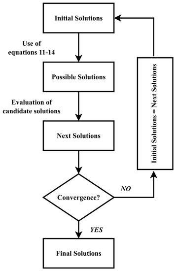
Figure 1.
Algorithmic Structure of Base Optimizing Algorithm applied for the optimization of the proposed regression models.
In this paper, BOA is used for the fine tuning of three different regression models used for short-term electricity price forecasting. More specifically, this metaheuristic algorithm is used to determine the appropriate values of the hyperparameters of an XGBoost model, an SVM and an MLP neural network that are used for prediction. The step of these models’ fine tuning, through the BOA, is particularly crucial as it aims to establish data driven models that will significantly enhance the prediction outcome of short-term electricity price forecasting.
3. Results
In this paper, the issue of short-term electricity price forecasting is examined using various optimized regression models in conjunction with the VMD approach or the K-Means clustering technique. For this reason, both ensembled preprocessing approaches are thoroughly examined separately by utilizing historical price data from the Greek electricity market as well as historical weather data consisting of hourly temperature and relative humidity values for the years 2017–2019. In order to fortuitously evaluate the data driven models and thoroughly compare the electricity price prediction results, the separation of the data into training and test sets has a rate of 80% and 20%, respectively. As previously mentioned, the models used for forecasting are an SVR, an MLP neural network and an XGBoost approach. The optimization of these regression models lies in the determination of their appropriate hyperparameters using BOA. The computer system used in this work for the development of the optimization algorithms and the preprocessing techniques, as well as for the evaluation of the proposed data-driven models, has an Intel Core i7-4510U at 2.00 GHz processor and an 8 GB installed memory.
3.1. Short-Term Electricity Price Forecasting Based on an Ensemble IDPSO-VMD Approach
In order to create a robust, data-driven forecasting model, which will display high accuracy in the electricity price forecasting results, the proposed IDPSO is utilized for the fine tuning of the VMD algorithm. Therefore, the number of IMFs in which the price signal is decomposed is not arbitrary, but is calculated from the maximization of Equation (2). Each resulting IMF is used by a regression model and then the individual results are combined in order to obtain the required price. The flowchart in Figure 2 illustrates in detail and clarity the proposed approach.
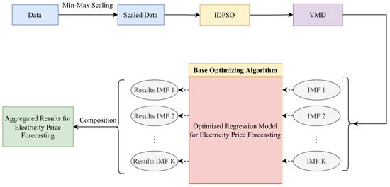
Figure 2.
Flowchart of the proposed STEPF approach in conjunction with the ensemble IDPSO-VMD algorithm.
In order to be able to deal with the EPF issue with accuracy and limited computational cost, the number of IMFs should be within a feasible range of values which is chosen arbitrarily. Table 1 gives the results of IDPSO-VMD within a certain range of K and values, as well as the values obtained by the remaining parameters of the algorithm. Figure 3 illustrates the decomposition of the scaled signal of the electricity price in the optimal number of IMFs, as derived from the IDPSO algorithm.

Table 1.
Optimization results of the enhanced VMD method based on the proposed IDPSO optimization technique.
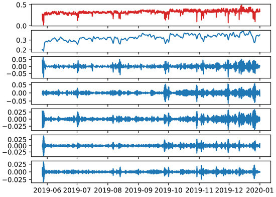
Figure 3.
Decomposition of the scaled signal of electricity price as a result of the IDPSO-VMD approach (Red: Initial signal; Blue: Decomposed IMFs).
Then, the optimization based on BOA is examined separately for each regression model that is proposed. The values from each of the IMFs obtained through the IDPSO-VMD approach are the input variables for a regression model. The individual results obtained from each model are evaluated based on two metrics that find extensive use in forecasting matters, the Mean Absolute Error (MAE) and the Mean Squared Error (MSE). In this particular approach, MAPE is not a safe comparison criterion as it takes very high values. This happens because the residuals resulting from the proposed decomposition method have values close to zero.
First, the case of an SVR is analyzed, due to their widespread use in the literature. It is emphasized that the hyperparameters that are free to choose in an SVR model are the type of kernel, the regularization parameter (C) and the epsilon () parameter. An MLP neural network is considered as the next regression model. The BOA is asked to determine the appropriate values of the neurons in the hidden layer and the number of epochs for each of the six neural networks deployed. Finally, this paper examines the effect that the implementation of an optimized XGBoost model will have on the result of the electricity price forecast. As previously mentioned, the XGBoost hyperparameters selected by BOA to create an optimized forecasting model are the learning rate, the maximum depth, the and parameters.
In Table 2, Table 3 and Table 4, the values of the hyperparameters of each SVM, MLP and XGBoost model, respectively, that utilize the data of the corresponding IMFs, as well as the results of the metrics for each IMF are aggregated. Figure 4, Figure 5 and Figure 6 illustrate the aggregated result of the forecast of electricity price using SVR, MLP and XGBoost models, respectively, in conjunction with the ensemble IDPSO-VMD algorithm.
Table 2.
BOA results for each SVR used in conjunction with the proposed IDPSO-VMD approach for STEPF.
Table 3.
BOA results for each MLP neural network used in conjunction with the proposed IDPSO-VMD approach for STEPF.
Table 4.
BOA results for each XGBoost model used in conjunction with the proposed IDPSO-VMD approach for STEPF.
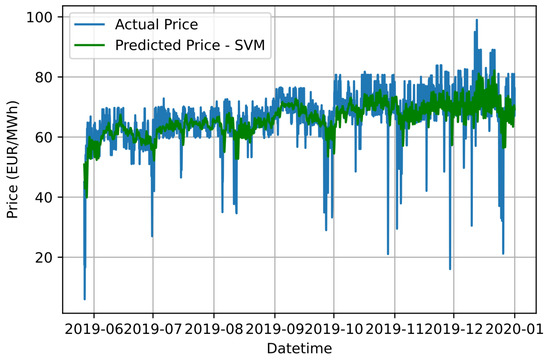
Figure 4.
Graphical comparison of forecasting results based on the proposed IDPSO-VMD-SVR approach and the actual electricity price values.
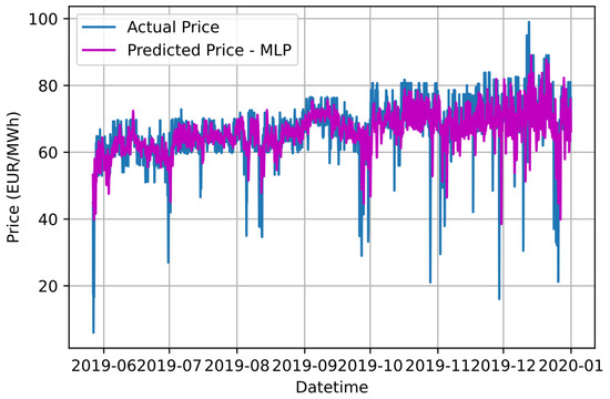
Figure 5.
Graphical comparison of forecasting results based on the proposed IDPSO-VMD-MLP approach and the actual electricity price values.
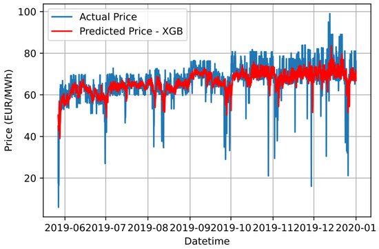
Figure 6.
Graphical comparison of forecasting results based on the proposed IDPSO-VMD-XGB approach and the actual electricity price values.
3.2. Short-Term Electricity Price Forecasting Based on an Ensemble K-Means Approach
In this work, the effect that the implementation of the K-Means clustering technique has on the result of price forecasting is examined. As in the previous approach, the number of clusters into which the data are divided is explicitly and thoroughly determined in order to apply the divide-and-conquer approach. Then, for each cluster, a regression model is used whose hyperparameters are optimized by BOA. Finally, the individual results are combined to obtain the desired STEPF result. Figure 7 illustrates the flowchart of this proposed approach.
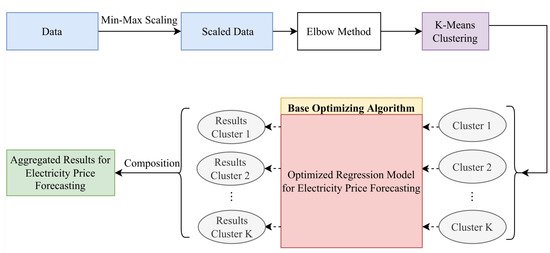
Figure 7.
Flowchart of the proposed STEPF approach in conjunction with the Ensemble K-Means clustering algorithm.
In the current work, the optimal number of clusters is determined using the Elbow Method. This approach requires the judgment and evaluation of the user to select the appropriate number of clusters. Therefore, two different users could choose a different K for the optimal number of clusters for the implementation of K-Means and therefore produce different results in the prediction. In this work, K accepts values between 2 and 8 because it is assumed that for more than 8 clusters, short-term electricity price forecasting cannot be addressed feasibly. Figure 8 illustrates the SSE for different numbers of clusters K. By applying the elbow approach, it is determined that 4 is the ideal number of clusters.
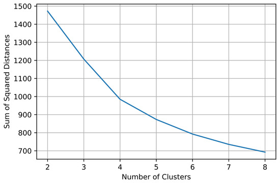
Figure 8.
Graphical representation of SSE values for a different number of clusters to decide the optimal value of K.
Similar to the previous approach, the regression models implemented for the STEPF issue are an SVR, an MLP neural network and an XGBoost model. The selection of their hyperparameters is achieved with the BAO metaheuristic technique. Table 5, Table 6 and Table 7 aggregate the hyperparameters for the SVR, MLPs and XGBoost models, respectively, used for each cluster, as well as the results of the metrics that each of them yields to the STEPF issue. In this approach, the prediction result of each cluster, apart from MAE and MSE, is calculated and evaluated based on MAPE. Figure 9, Figure 10 and Figure 11 illustrate the aggregated result of the forecast of electricity price using SVR, MLP and XGBoost models, respectively, in conjunction with the Ensemble K-Means clustering technique.
Table 5.
BOA results for each SVR used in conjunction with the Ensemble K-Means approach for STEPF.
Table 6.
BOA results for each MLP neural network used in conjunction with the Ensemble K-Means approach for STEPF.
Table 7.
BOA results for each XGBoost model used in conjunction with the Ensemble K-Means approach for STEPF.
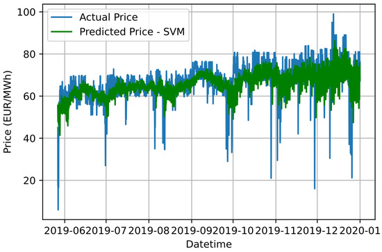
Figure 9.
Graphical comparison of forecasting results based on the proposed Ensemble K-Means-SVR approach and the actual electricity price values.
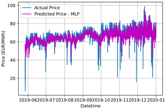
Figure 10.
Graphical comparison of forecasting results based on the proposed Ensemble K-Means-MLP approach and the actual electricity price values.
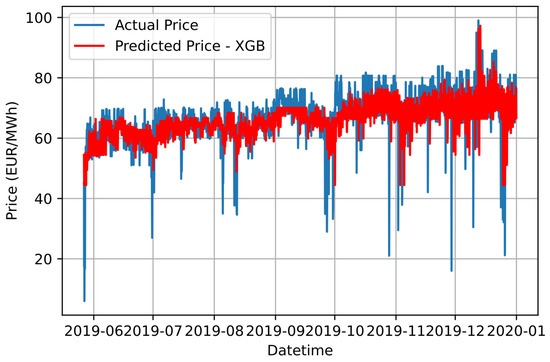
Figure 11.
Graphical comparison of forecasting results based on the proposed Ensemble K-Means-XGB approach and the actual electricity price values.
This work presents a thorough comparison of the results that both signal decomposition and clustering techniques can bring to STEPF. Table 8 aggregates the results of the metrics obtained from the implementation of all three proposed regressor models in conjunction with the IDPSO-VMD algorithm and from the implementation of the Ensemble K-Means, respectively. Figure 12 is a comparison of the proposed methods in terms of the MAPE metric.
Table 8.
Aggregate results of the metrics for each proposed electricity price forecasting method.
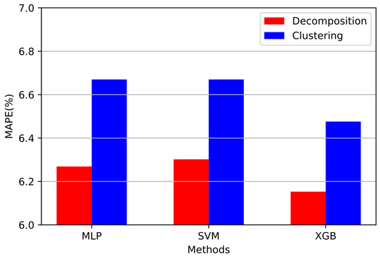
Figure 12.
Bar chart for visual comparison of MAPE values of each proposed electricity price forecasting algorithm.
4. Discussion
In this paper, two novel and robust approaches for short-term price forecasting using historical electricity prices are proposed. Although the proposed methods can be applied to any forecasting approach, in this work their accuracy is examined using data from the Greek deregulated electricity market. The results based on the metrics which are summarized in Table 8 and Figure 12 will be discussed in the current section in order to conduct a comparative analysis between the effect of signal decomposition and the effect of the clustering technique on STEPF.
First, the proposed technique that produces the smallest error in the forecast is IDPSO-VMD-XGB with an MAPE value of 6.15%. The proposed IDPSO-VMD-XGB data-driven model, compared to the rest of the models examined, brings the highest accuracy to the STEPF issue in the shortest convergence time. Morevoer, it is concluded that in both approaches the regressor model that produces the most accurate results and therefore the lowest MAPE value is the XGBoost model. Next come the MLP neural networks that perform more accurately in predicting the electricity price compared to the SVRs that are extensively used in the literature. The comparison regarding the accuracy of all the proposed methods can be conducted safely as all the regressor models used in electricity price forecasting have been optimized using BOA as a front-end metaheuristic algorithm. In addition, in the approach where signal decomposition is used as a preprocessing technique, the regression models used in the prediction bring more accurate results compared to their peers that are implemented in conjunction with the Ensemble K-Means clustering technique. This conclusion is also observed from Figure 12 where the red bars are lower compared to the corresponding blue ones. By observing Figure 4, Figure 5 and Figure 6 and Figure 9, Figure 10 and Figure 11, it can be distinguished that the proposed approaches cannot accurately generalize in the price drops observed in the Greek electricity market. These price drops are mainly due to exogenous factors and therefore should be treated differently in the electricity price forecast. Therefore, as future work, a model specializing in the price drops of the Greek electricity market could be designed, which in conjunction with the proposed IDPSO-VMD-XGB model will bring even greater accuracy to the electricity price forecast issue.
5. Conclusions
In this paper, we address the short-term electricity price forecasting issue by developing and implementing six robust and optimized data-driven forecasting models in conjunction with the Variational Mode Decomposition or the K-Means approach. In order to confirm the high accuracy of the proposed approaches, the prediction outcomes, that yield from their application on the short-term electricity price forecasting issue, are thoroughly compared in terms of accuracy by calculating the MAE, MSE and MAPE scores. At the same time, an enhanced IDPSO optimization algorithm is developed for the selection of the optimal values of the VMD’s hyperparameters. The optimization of the regressor models used for short-term electricity price forecasting, using the data of the deregulated Greek electricity market, is achieved via the BOA metaheuristic algorithm. This paper fills the gap that exists in the literature for the comparison between signal decomposition and clustering as preprocessing approaches used by hybrid models of electricity price prediction. Based on a thorough comparison of the forecasting results, it is clear that signal decomposition of the electricity price produces more accurate results than data clustering methods and should thus be preferred as a preprocessing approach when developing hybrid forecasting models that are implemented in the STEPF, while the IDPSO-VMD-XGB model, with an MAPE value of 6.15%, is the proposed method that results in the lowest prediction error. As future work, the creation of appropriate forecasting models will be investigated in order to generalize effectively in circumstances when price decreases (or spikes) arise in the electricity price curve, resulting in even more accurate predicting results.
Author Contributions
Conceptualization, A.I.A.; methodology, A.I.A.; software, A.I.A.; validation, A.I.A., D.B. and M.A.; formal analysis, A.I.A.; investigation, A.I.A.; resources, A.I.A., D.K., A.F. and M.A.; data curation, A.I.A., D.K., A.F. and M.A.; writing—original draft preparation, A.I.A.; writing—review and editing, A.I.A., D.B. and M.A.; visualization, A.I.A., D.K., A.F. and M.A.; supervision, D.B. and M.A.; project administration, D.B. and M.A. All authors have read and agreed to the published version of the manuscript.
Funding
This research received no external funding.
Institutional Review Board Statement
Not applicable.
Informed Consent Statement
Not applicable.
Data Availability Statement
Data are available in a publicly accessible repository. The data used in this study are openly available from the ENTSO-E portal in https://open-power-system-data.org/data-sources, accessed on 18 April 2022. The dataset was processed as the input for the design and performance assessment of the proposed data-driven forecasting models described in this article.
Conflicts of Interest
The authors declare no conflict of interest.
References
- Necoechea-Porras, P.D.; Lopez, A.; Salazar-Elena, J.C. Deregulation in the Energy Sector and Its Economic Effects on the Power Sector: A Literature Review. Sustainability 2021, 13, 3429. [Google Scholar] [CrossRef]
- Cramton, P. Electricity market design: The good, the bad and the ugly. In Proceedings of the 36th Annual Hawaii International Conference on System Sciences, Big Island, HI, USA, 6–9 January 2003; p. 8. [Google Scholar] [CrossRef]
- Shahidehpour, M.; Yamin, H.; Li, Z. Electricity Price Forecasting. In Market Operations in Electric Power Systems: Forecasting, Scheduling and Risk Management; John Wiley & Sons, Inc.: New York, NY, USA, 2002; pp. 57–113. [Google Scholar] [CrossRef]
- Weron, R. Electricity price forecasting: A review of the state-of-the-art with a look into the future. Int. J. Forecast. 2014, 30, 1030–1081. [Google Scholar] [CrossRef]
- Arvanitidis, A.I.; Bargiotas, D.; Daskalopulu, A.; Laitsos, V.M.; Tsoukalas, L.H. Enhanced Short-Term Load Forecasting Using Artificial Neural Networks. Energies 2021, 14, 7788. [Google Scholar] [CrossRef]
- Kontogiannis, D.; Bargiotas, D.; Daskalopulu, A. Minutely Active Power Forecasting Models Using Neural Networks. Sustainability 2020, 12, 3177. [Google Scholar] [CrossRef]
- Weber, C. Uncertainty in the Electric Power Industry; Number 978-0-387-23048-1 in International Series in Operations Research and Management Science; Springer: New York, NY, USA, 2005. [Google Scholar] [CrossRef]
- Manner, H.; Türk, D.; Eichler, M. Modeling and forecasting multivariate electricity price spikes. Energy Econ. 2016, 60, 255–265. [Google Scholar] [CrossRef]
- Sirin, S.M.; Erten, I. Price spikes, temporary price caps and welfare effects of regulatory interventions on wholesale electricity markets. Energy Policy 2022, 163, 112816. [Google Scholar] [CrossRef]
- Liu, S.; Jiang, Y.; Lin, Z.; Wen, F.; Ding, Y.; Yang, L. Data-driven two-step day-ahead electricity price forecasting considering price spikes. J. Mod. Power Syst. Clean Energy 2022. [Google Scholar] [CrossRef]
- Kontogiannis, D.; Bargiotas, D.; Daskalopulu, A.; Arvanitidis, A.I.; Tsoukalas, L.H. Error Compensation Enhanced Day-Ahead Electricity Price Forecasting. Energies 2022, 15, 1466. [Google Scholar] [CrossRef]
- Cerjan, M.; Krželj, I.; Vidak, M.; Delimar, M. A literature review with statistical analysis of electricity price forecasting methods. In Proceedings of the Eurocon 2013, Zagreb, Croatia, 1–4 July 2013; pp. 756–763. [Google Scholar] [CrossRef]
- Duch, W.; Setiono, R.; Zurada, J. Computational intelligence methods for rule-based data understanding. Proc. IEEE 2004, 92, 771–805. [Google Scholar] [CrossRef]
- Jakaša, T.; Andročec, I.; Sprčić, P. Electricity price forecasting—ARIMA model approach. In Proceedings of the 2011 8th International Conference on the European Energy Market (EEM), Zagreb, Croatia, 25–27 May 2011; pp. 222–225. [Google Scholar] [CrossRef]
- Carpio, J.; Juan, J.; López, D. Multivariate Exponential Smoothing and Dynamic Factor Model Applied to Hourly Electricity Price Analysis. Technometrics 2014, 56, 494–503. [Google Scholar] [CrossRef]
- Jónsson, T.; Pinson, P.; Nielsen, H.A.; Madsen, H. Exponential Smoothing Approaches for Prediction in Real-Time Electricity Markets. Energies 2014, 7, 3710–3732. [Google Scholar] [CrossRef]
- Tsampasis, E.; Bargiotas, D.; Elias, C.; Sarakis, L. Communication challenges in Smart Grid. MATEC Web Conf. 2016, 41, 01004. [Google Scholar] [CrossRef]
- Lahmiri, S. Comparing Variational and Empirical Mode Decomposition in Forecasting Day-Ahead Energy Prices. IEEE Syst. J. 2017, 11, 1907–1910. [Google Scholar] [CrossRef]
- Ribeiro, M.H.D.M.; Stefenon, S.F.; de Lima, J.D.; Nied, A.; Mariani, V.C.; Coelho, L.d.S. Electricity Price Forecasting Based on Self-Adaptive Decomposition and Heterogeneous Ensemble Learning. Energies 2020, 13, 5190. [Google Scholar] [CrossRef]
- Qiu, X.; Suganthan, P.; Amaratunga, G.A. Short-term Electricity Price Forecasting with Empirical Mode Decomposition based Ensemble Kernel Machines. Procedia Comput. Sci. 2017, 108, 1308–1317. [Google Scholar] [CrossRef]
- Khan, S.; Aslam, S.; Mustafa, I.; Aslam, S. Short-Term Electricity Price Forecasting by Employing Ensemble Empirical Mode Decomposition and Extreme Learning Machine. Forecasting 2021, 3, 460–477. [Google Scholar] [CrossRef]
- Sun, G.; Chen, T.; Wei, Z.; Sun, Y.; Zang, H.; Chen, S. A Carbon Price Forecasting Model Based on Variational Mode Decomposition and Spiking Neural Networks. Energies 2016, 9, 54. [Google Scholar] [CrossRef]
- Huang, Y.; Deng, Y. A new crude oil price forecasting model based on variational mode decomposition. Knowl.-Based Syst. 2021, 213, 106669. [Google Scholar] [CrossRef]
- Wang, R.; Li, C.; Fu, W.; Tang, G. Deep Learning Method Based on Gated Recurrent Unit and Variational Mode Decomposition for Short-Term Wind Power Interval Prediction. IEEE Trans. Neural Netw. Learn. Syst. 2020, 31, 3814–3827. [Google Scholar] [CrossRef]
- Yang, W.; Wang, J.; Niu, T.; Du, P. A novel system for multi-step electricity price forecasting for electricity market management. Appl. Soft Comput. 2020, 88, 106029. [Google Scholar] [CrossRef]
- Wang, J.; Yang, W.; Du, P.; Niu, T. Outlier-robust hybrid electricity price forecasting model for electricity market management. J. Clean. Prod. 2020, 249, 119318. [Google Scholar] [CrossRef]
- Ghayekhloo, M.; Azimi Asiabar, R.; Ghofrani, M.; Menhaj, M.; Shekari, E. A combination approach based on a novel data clustering method and Bayesian Recurrent Neural Network for day-ahead price forecasting of electricity markets. Electr. Power Syst. Res. 2018, 168, 184–199. [Google Scholar] [CrossRef]
- Pourhaji, N.; Asadpour, M.; Ahmadian, A.; Elkamel, A. The Investigation of Monthly/Seasonal Data Clustering Impact on Short-Term Electricity Price Forecasting Accuracy: Ontario Province Case Study. Sustainability 2022, 14, 3063. [Google Scholar] [CrossRef]
- Wang, F.; Li, K.; Zhou, L.; Ren, H.; Contreras, J.; Shafie-khah, M.; Catalão, J. Daily pattern prediction based classification modeling approach for day-ahead electricity price forecasting. Int. J. Electr. Power Energy Syst. 2019, 105, 529–540. [Google Scholar] [CrossRef]
- Huang, N.E.; Shen, Z.; Long, S.R.; Wu, M.C.; Shih, H.H.; Zheng, Q.; Yen, N.C.; Tung, C.C.; Liu, H.H. The Empirical Mode Decomposition and the Hilbert spectrum for nonlinear and non-stationary time series analysis. Proc. R. Soc. Lond. Ser. A 1998, 454, 903–998. [Google Scholar] [CrossRef]
- Rato, R.; Ortigueira, M.; Batista, A. On the HHT, its problems and some solutions. Mech. Syst. Signal Process. 2008, 22, 1374–1394. [Google Scholar] [CrossRef]
- Feldman, M. Time-varying vibration decomposition and analysis based on the Hilbert transform. J. Sound Vib. 2006, 295, 518–530. [Google Scholar] [CrossRef]
- Braun, S.; Feldman, M. Decomposition of non-stationary signals into varying time scales: Some aspects of the EMD and HVD methods. Mech. Syst. Signal Process. 2011, 25, 2608–2630. [Google Scholar] [CrossRef]
- Rilling, G.; Flandrin, P. One or Two Frequencies? The Empirical Mode Decomposition Answers. IEEE Trans. Signal Process. 2008, 56, 85–95. [Google Scholar] [CrossRef]
- Torres, M.E.; Colominas, M.A.; Schlotthauer, G.; Flandrin, P. A complete ensemble Empirical Mode Decomposition with adaptive noise. In Proceedings of the 2011 IEEE International Conference on Acoustics, Speech and Signal Processing (ICASSP), Prague, Czech Republic, 22–27 May 2011; pp. 4144–4147. [Google Scholar] [CrossRef]
- Civera, M.; Surace, C. A Comparative Analysis of Signal Decomposition Techniques for Structural Health Monitoring on an Experimental Benchmark. Sensors 2021, 21, 1825. [Google Scholar] [CrossRef]
- Dragomiretskiy, K.; Zosso, D. Variational Mode Decomposition. IEEE Trans. Signal Process. 2014, 62, 531–544. [Google Scholar] [CrossRef]
- Zhang, D.; Feng, Z. Application of Variational Mode Decomposition based demodulation Analysis in gearbox fault diagnosis. In Proceedings of the 2016 IEEE International Instrumentation and Measurement Technology Conference Proceedings, Taipei, Taiwan, 23–26 May 2016; pp. 1–6. [Google Scholar] [CrossRef]
- Yi, C.; Lv, Y.; Zhang, D. A Fault Diagnosis Scheme for Rolling Bearing Based on Particle Swarm Optimization in Variational Mode Decomposition. Shock Vib. 2016, 2016, 9372691. [Google Scholar] [CrossRef]
- Liu, W.; Cao, S.; Chen, Y. Applications of Variational Mode Decomposition in seismic time-frequency analysis. Geophysics 2016, 81, V365–V378. [Google Scholar] [CrossRef]
- Li, T.; Qian, Z.; Deng, W.; Zhang, D.; Lu, H.; Wang, S. Forecasting crude oil prices based on Variational Mode Decomposition and random sparse Bayesian learning. Appl. Soft Comput. 2021, 113, 108032. [Google Scholar] [CrossRef]
- Zhang, G.; Xu, B.; Liu, H.; Hou, J.; Zhang, J. Wind Power Prediction Based on Variational Mode Decomposition and Feature Selection. J. Mod. Power Syst. Clean Energy 2021, 9, 1520–1529. [Google Scholar] [CrossRef]
- Zhou, M.; Hu, T.; Bian, K.; Lai, W.; Hu, F.; Hamrani, O.; Zhu, Z. Short-Term Electric Load Forecasting Based on Variational Mode Decomposition and Grey Wolf Optimization. Energies 2021, 14, 4890. [Google Scholar] [CrossRef]
- Peng, Z.; Wei, K.; Tian, W.; Shi, P.; Yang, W. Superiorities of Variational Mode Decomposition over Empirical Mode Decomposition Particularly in Time-frequency Feature Extraction and Wind Turbine Condition Monitoring. IET Renew. Power Gener. 2016, 11, 443–452. [Google Scholar] [CrossRef]
- Liu, Y.; Yang, G.; Li, M.; Yin, H. Variational Mode Decomposition Denoising Combined the Detrended Fluctuation Analysis. Signal Process. 2016, 125, 349–364. [Google Scholar] [CrossRef]
- Bagheri, A.; Ozbulut, O.E.; Harris, D.K. Structural system identification based on variational mode decomposition. J. Sound Vib. 2018, 417, 182–197. [Google Scholar] [CrossRef]
- Sahani, M.; Dash, P.; Samal, D. A real-time power quality events recognition using variational mode decomposition and online-sequential Extreme Learning Machine. Measurement 2020, 157, 107597. [Google Scholar] [CrossRef]
- Wang, X.B.; Yang, Z.X.; Yan, X.A. Novel Particle Swarm Optimization-Based Variational Mode Decomposition Method for the Fault Diagnosis of Complex Rotating Machinery. IEEE/ASME Trans. Mechatron. 2018, 23, 68–79. [Google Scholar] [CrossRef]
- Lin, Y.; Xiao, M.; Liu, H.; Li, Z.; Zhou, S.; Xu, X.; Wang, D. Gear fault diagnosis based on CS-improved variational mode decomposition and probabilistic neural network. Measurement 2022, 192, 110913. [Google Scholar] [CrossRef]
- Zhang, X.; Li, D.; Li, J.; Li, Y. Grey wolf optimization-based Variational Mode Decomposition for magnetotelluric data combined with detrended fluctuation analysis. Acta Geophys. 2022, 70, 111–120. [Google Scholar] [CrossRef]
- Fu, W.; Wang, K.; Li, X.; Li, Y.; Zhong, H. Vibration trend measurement for hydropower generator based on optimal Variational Mode Decomposition and LSSVM improved with chaotic sine cosine algorithm optimization. Meas. Sci. Technol. 2018, 30, 015012. [Google Scholar] [CrossRef]
- Kennedy, J.; Eberhart, R. Particle Swarm Optimization. In Proceedings of the ICNN’95–International Conference on Neural Networks, Perth, Australia, 27 November–1 December 1995; Volume 4, pp. 1942–1948. [Google Scholar] [CrossRef]
- Wang, S.; Wang, L.; Pi, Y. A hybrid differential evolution algorithm for a stochastic location-inventory-delivery problem with joint replenishment. Data Sci. Manag. 2022, 5, 124–136. [Google Scholar] [CrossRef]
- Wu, B.; Wang, L.; Zeng, Y.R. Interpretable wind speed prediction with multivariate time series and temporal fusion transformers. Energy 2022, 252, 123990. [Google Scholar] [CrossRef]
- Peng, L.; Sun, C.; Wu, W. Effective arithmetic optimization algorithm with probabilistic search strategy for function optimization problems. Data Sci. Manag. 2022. [Google Scholar] [CrossRef]
- Wang, H.D.; Deng, S.E.; Yang, J.X.; Liao, H.; Li, W.B. Parameter-Adaptive VMD Method Based on BAS Optimization Algorithm for Incipient Bearing Fault Diagnosis. Math. Probl. Eng. 2020, 2020, 5659618. [Google Scholar] [CrossRef]
- Liang, T.; Lu, H.; Sun, H. Application of Parameter Optimized Variational Mode Decomposition Method in Fault Feature Extraction of Rolling Bearing. Entropy 2021, 23, 520. [Google Scholar] [CrossRef]
- Choudhury, D. Teaching the concept of convolution and correlation using Fourier transform. In Proceedings of the 14th Conference on Education and Training in Optics and Photonics: ETOP 2017, Hangzhou, China, 29–31 May 2017; Liu, X., Zhang, X.C., Eds.; International Society for Optics and Photonics, SPIE: Bellingham, WA, USA, 2017; Volume 10452, pp. 183–188. [Google Scholar] [CrossRef][Green Version]
- Pedregosa, F.; Varoquaux, G.; Gramfort, A.; Michel, V.; Thirion, B.; Grisel, O.; Blondel, M.; Prettenhofer, P.; Weiss, R.; Dubourg, V.; et al. Scikit-learn: Machine Learning in Python. J. Mach. Learn. Res. 2011, 12, 2825–2830. [Google Scholar]
- Hearst, M.; Dumais, S.; Osman, E.; Platt, J.; Scholkopf, B. Support Vector Machines. Intell. Syst. Their Appl. IEEE 1998, 13, 18–28. [Google Scholar] [CrossRef]
- Shmilovici, A. Support Vector Machines. In Data Mining and Knowledge Discovery Handbook; Maimon, O., Rokach, L., Eds.; Springer: Boston, MA, USA, 2010; pp. 231–247. [Google Scholar] [CrossRef]
- Awad, M.; Khanna, R. Support Vector Regression. In Efficient Learning Machines: Theories, Concepts and Applications for Engineers and System Designers; Apress: Berkeley, CA, USA, 2015; pp. 67–80. [Google Scholar] [CrossRef]
- Smola, A.; Schölkopf, B. A tutorial on Support Vector Regression. Stat. Comput. 2004, 14, 199–222. [Google Scholar] [CrossRef]
- Chen, T.; Guestrin, C. XGBoost: A Scalable Tree Boosting System. In Proceedings of the 22nd ACM SIGKDD International Conference on Knowledge Discovery and Data Mining, San Francisco, CA, USA, 13–17 August 2016; Association for Computing Machinery: New York, NY, USA, 2016. KDD ’16. pp. 785–794. [Google Scholar] [CrossRef]
- Breiman, L.; Friedman, J.H.; Olshen, R.A.; Stone, C.J. Classification and Regression Trees; Routledge: New York, NY, USA, 1983. [Google Scholar]
- Bentéjac, C.; Csörgo, A.; Martínez-Muñoz, G. A Comparative Analysis of Gradient Boosting Algorithms. Artif. Intell. Rev. 2021, 54, 1937–1967. [Google Scholar] [CrossRef]
- Arvanitidis, A.I.; Bargiotas, D. Use of Artificial Neural Networks for Short Term Load Forecasting. In Proceedings of the 25th Pan-Hellenic Conference on Informatics, Volos, Greece, 26–28 November 2021; Association for Computing Machinery: New York, NY, USA, 2021. PCI 2021. pp. 18–22. [Google Scholar] [CrossRef]
- Meyer-Baese, A.; Schmid, V. Chapter 7–Foundations of Neural Networks. In Pattern Recognition and Signal Analysis in Medical Imaging, 2nd ed.; Meyer-Baese, A., Schmid, V., Eds.; Academic Press: Oxford, UK, 2014; pp. 197–243. [Google Scholar] [CrossRef]
- Wilamowski, B.; Chen, Y.; Malinowski, A. Efficient algorithm for training neural networks with one hidden layer. In Proceedings of the IJCNN’99. International Joint Conference on Neural Networks, Proceedings (Cat. No.99CH36339), Washington, DC, USA, 10–16 July 1999; Volume 3, pp. 1725–1728. [Google Scholar] [CrossRef]
- Glover, F. Future paths for integer programming and links to artificial intelligence. Comput. Oper. Res. 1986, 13, 533–549. [Google Scholar] [CrossRef]
- Blum, C.; Roli, A. Metaheuristics in Combinatorial Optimization: Overview and Conceptual Comparison. ACM Comput. Surv. 2003, 35, 268–308. [Google Scholar] [CrossRef]
- Salem, S.A. BOA: A novel optimization algorithm. In Proceedings of the 2012 International Conference on Engineering and Technology (ICET), Cairo, Egypt, 10–11 October 2012; pp. 1–5. [Google Scholar] [CrossRef]


Publisher’s Note: MDPI stays neutral with regard to jurisdictional claims in published maps and institutional affiliations. |
© 2022 by the authors. Licensee MDPI, Basel, Switzerland. This article is an open access article distributed under the terms and conditions of the Creative Commons Attribution (CC BY) license (https://creativecommons.org/licenses/by/4.0/).