Investigation of the Effect of Albedo in Photovoltaic Systems for Urban Applications: Case Study for Spain

Abstract

Rooftop photovoltaic generation can help cities become key players in the transition to clean energy. The optimal solar photovoltaic production on rooftops depends on two angles: tilt angle and azimuth angle. It is accepted in all studies that the ideal orientation of photovoltaic modules is toward the south (north) in the northern hemisphere (south). In contrast, the determination of the optimum tilt angle is more complex, and there are different equations for its calculation. Most of these equations do not take albedo into account. In this work, 47 Spanish province capitals representing the most populated cities have been studied with different equations for the calculation of the optimum annual tilt angle (Technical report by the Spanish Institute for the Diversification and Saving of Energy (IDAE), Lorenzo’s and Jacobson’s equation) and different types of albedo. Accounting for the geographical and the meteorological conditions of the cities, we analyzed the optimum tilt angle through a Mathematica© optimization code. The influence that different variables have on optimum tilt angle has been quantified by means of the term relative energy harvested. The use of the equations as a function of latitude increases the annual relative energy harvested by increasing the albedo. When the albedo is 0.2, the annual relative energy harvested is very similar in all equations. Comparing to the method that maximizes the total irradiation incident on a tilted surface, the minimum and maximum value of the percentage of relative energy harvested per year were 0.01 and 2.50% for the IDAE guideline, 0.00 and 2.38% for Lorenzo’s equation, 0.00 and 2.46% for Jacobson’s equation. A simplified polynomial regression model to estimate optimum tilt angle as a function of latitude, altitude and albedo has been proposed as well.

1. Introduction

Electricity generation is the engine of the economic and social development of society. The need for large amounts of electrical energy has led to unprecedented environmental issues due to the use of fossil fuels and therefore the increasing of greenhouse gas emissions. There is a global consensus to reduce the use of fossil fuels and replace it with renewable energy sources of energy [1]. It is the called clean energy transition. A long-term sustainable energy model is therefore necessary to meet the commitments made by governments at the global level.

Solar energy is a renewable energy source that can be used for electricity generation. Electricity can be generated directly by photovoltaic systems [2] or by converting the Sun’s energy into high-temperature heat (concentrating solar power plants) [3]. From the point of view of their use in cities, the first technology is the right one.

Cities are major players in the environmental issues considered as examples of unsustainability [4]. Buildings in the European Union ($EU$) are responsible for $40\%$ of final energy consumption and $36\%$ of greenhouse gas emissions [5]. For this reason, cities are at the center of the implementation of $EU$ policies [6] such as the promotion of low and zero-energy buildings. In this scenario, cities need profound changes toward an ecological future [7].

The decentralized electricity production ($DEP$) systems can help make cities key players in the clean energy transition. This new paradigm of electricity production is revolutionizing the power generation sector [8]. In this sense, Gómez et al. [9] introduce the concept of “prosumer”, or a customer who consumes and can sell generated electricity. Electricity production by means of building-integrated photovoltaics systems and building-applied photovoltaics systems are two solutions used in $DEP$ systems.

The installation of $PV$ systems on rooftops is rapidly growing [10], as they produce benefits from various points of view: health [11], environmental [12], economic [13], and social [14]. These systems have been studied by several authors [15,16].

The optimal solar $PV$ production on rooftops depends on two angles [17]: the angle between the plane of the $PV$ module and the horizontal plane (called tilt angle $\beta$) and the angle between the projection on a horizontal plane of the normal to the $PV$ module and south direction (called azimuth angle $\gamma$). These angles not only have a direct impact on the amount of solar irradiance incident on a $PV$ module [18] but also influence the surface area required for the installation of the PV system [19]. The optimum azimuth angle for tilted surfaces is facing due south (north) in the northern (southern) hemisphere [17]. Many researchers have studied procedures to find the optimum tilt angle, grouping them into two categories.

The first category uses equations based on the latitude, in which the optimum tilt angle is taken as the latitude plus or minus a specific value obtained via analytic methods (e.g., regression analysis). These equations are very easy to use but prone to error. In addition, these equations have been determined for albedos close to $0.2$. Yet in the building sector, materials with albedos greater than $0.2$ can be used. Therefore, the use of these equations leads to errors in the estimation of the energy absorbed by the PV modules. These equations are used as an installation guide of $PV$ modules in practical engineering applications.

A large number of studies belong to this first category. Ullah et al. [20] showed a detailed summary of these studies. These studies were carried out with the aim of obtaining formulas to determine the optimum tilt angle of $PV$ modules. For locations with $\lambda <45$$°$ (where $\lambda$ is the latitude of the site), Lorenzo [21] obtained the optimal tilt of solar collector as a function of latitude: ${\beta }_{opt}=3.7+0.69·\left|\lambda \right|$. Jacobson et al. [22] carried out an analysis that includes a 3rd degree polynomial: ${\beta }_{opt}=1.3793+\lambda (1.2011+\lambda (-0.014404+0.000080509\lambda ))$. These two studies do not take into account the variation of the albedo. Nicolás-Martín et al. [23] obtained the annual optimum tilt angle as a function of latitude, diffuse fraction and albedo. To do this, $\mathrm{14,468}$ sites spread across the globe from the One Building database were used. Their study did take into account the albedo variation.

The second category cover procedures that maximize the total solar irradiance incident on a tilted surface over a period of time. These procedures are more accurate, yet they are more complex. Soulayman et al. [24] presented a modified general algorithm to determine the annual optimum tilt angle over all mid-latitude zone. The latitude of these sites varied between $23.45$ ($°$) N and $43.45$ ($°$) N and between $23.45$ ($°$) S and $43.45$ ($°$) S. This work suggested following equation ${\beta }_{opt}=1.171+0.916·\lambda$ for the mid-latitudes zone of the northern hemisphere. Al Garni et al. [25] investigated the annual optimum tilt angle of $PV$ modules for 18 sites of Saudi Arabia. The latitude of the cities varied between $18.22$ ($°$) and $31.02$ ($°$). For these sites, the optimal tilt was only slightly higher than the latitude. Ullah et al. [20] investigated the annual optimum tilt angle for $PV$ modules for several cities in Pakistan. This study was experimentally validated for one of the cities studied. Barbón et al. [2], applying Cavaleri’s principle, investigates the annual optimum tilt angles for $PV$ modules for 39 locations in the northern hemisphere. These four studies do not take into account the variation of the albedo.

Table 1. Advantages and disadvantages of procedures to find optimum tilt angle.

Parameter	Equations Based on the Latitude	Maximise the Total Solar Irradiance Incident
Easy to use	Advantage	Disadvantage
Prone to error	Disadvantage	Advantage
Albedo variation	Disadvantage	Advantage

shows a summary of the advantages and disadvantages of procedures to find the optimum tilt angle.

The objective of this paper is to study the influence that several variables have on the optimum tilt angle for 47 Spanish province capitals and to propose equations that estimate the optimum tilt angle that take into account the variations of the albedo. The notable difference with the methods in the first category is that our procedure allows the albedo value to be varied. The analysis is performed using an algorithm that maximizes the solar irradiation reaching the tilted surface for a given period of time. The annual optimum tilt angle for each of the cities is computed using Cavaleri’s principle. The influence that the different variables have on optimum tilt angle is quantified by means of the term relative energy harvesting ($REH$). $REH$ can be defined as the ratio of the energy collected through the direct application of each model to the amount obtained by application of Cavaleri’s principle.

The specific contributions of this study can be summarized as follows:

(i)

We analyze the equations proposed by the Spanish regulations for the determination of the annual optimum tilt angle.

(ii)

We determine the error caused through the use of the equations based on the latitude that do not take into account the variation of the albedo.

(iii)

We propose a method to compute the annual optimum tilt angle that accounts for the albedo variations.

(iv)

We conduct a detailed analysis of the relative energy harvesting as a function of different variables.

(v)

Finally, a simplified polynomial regression model to estimate optimum tilt angle as a function of latitude, altitude and albedo is proposed.

This paper is organized as follows: the geographic characteristics of the Spanish province capitals are presented in Section 2. Section 3 presents the solar irradiance estimation model and the procedure followed to calculate the amount of total irradiation on a tilted plane. The methods used to calculate the optimum tilt angle are described in Section 4. Section 5 presents the results of the study. Finally, Section 6 summarizes the main contributions and conclusions of the paper.

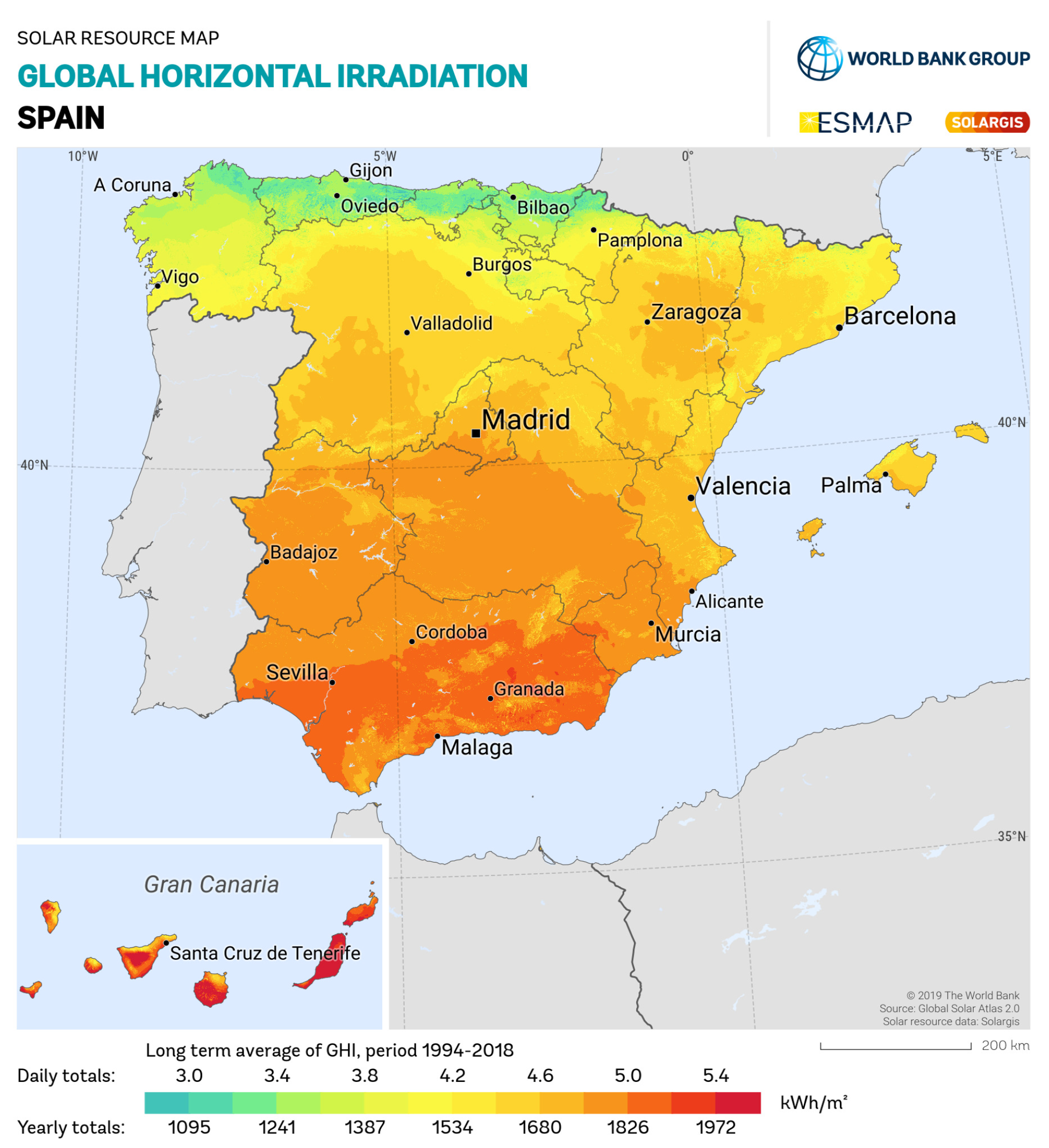
2. A Case Study in Spain

A total number of 47 province capitals comprising $29.8\%$ of the Spanish population have been analyzed, representing the most populous cities of Spain. These locations are given in

Table 2. Cities under study.

Id	City	Latitude	Longitude	Alt. (m)
1	Cádiz	36$°$32${}^{\prime }$06${}^{″}$ N	06$°$17${}^{\prime }$51${}^{″}$ W	13
2	Málaga	36$°$43${}^{\prime }$00${}^{″}$ N	04$°$25${}^{\prime }$00${}^{″}$ W	8
3	Almería	36$°$50${}^{\prime }$00${}^{″}$ N	0$2°$27${}^{\prime }$00${}^{″}$ W	16
4	Granada	37$°$10${}^{\prime }$41${}^{″}$ N	03$°$36${}^{\prime }$03${}^{″}$ W	684
5	Huelva	37$°$15${}^{\prime }$00${}^{″}$ N	06$°$57${}^{\prime }$00${}^{″}$ W	24
6	Sevilla	37$°$23${}^{\prime }$00${}^{″}$ N	05$°$59${}^{\prime }$00${}^{″}$ W	11
7	Jaén	37$°$46${}^{\prime }$11${}^{″}$ N	03$°$47${}^{\prime }$20${}^{″}$ W	570
8	Córdoba	37$°$53${}^{\prime }$00${}^{″}$ N	04$°$46${}^{\prime }$00${}^{″}$ W	106
9	Murcia	37$°$59${}^{\prime }$10${}^{″}$ N	0$1°$07${}^{\prime }$49${}^{″}$ W	42
10	Alicante	38$°$20${}^{\prime }$43${}^{″}$ N	00$°$28${}^{\prime }$59${}^{″}$ W	5
11	Badajoz	38$°$52${}^{\prime }$49${}^{″}$ N	06$°$58${}^{\prime }$31${}^{″}$ W	182
12	Ciudad Real	38$°$59${}^{\prime }$00${}^{″}$ N	03$°$55${}^{\prime }$00${}^{″}$ W	625
13	Albacete	38$°$59${}^{\prime }$44${}^{″}$ N	01$°$51${}^{\prime }$21${}^{″}$ W	681
14	Valencia	39$°$28${}^{\prime }$00${}^{″}$ N	00$°$22${}^{\prime }$30${}^{″}$ W	16
15	Cáceres	39$°$28${}^{\prime }$23${}^{″}$ N	06$°$22${}^{\prime }$16${}^{″}$ W	457
16	Toledo	39$°$52${}^{\prime }$00${}^{″}$ N	04$°$02${}^{\prime }$00${}^{″}$ W	516
17	Castellón	39$°$58${}^{\prime }$00${}^{″}$ N	00$°$03${}^{\prime }$00${}^{″}$ W	27
18	Cuenca	40$°$04${}^{\prime }$18${}^{″}$ N	02$°$08${}^{\prime }$06${}^{″}$ W	997
19	Teruel	40$°$20${}^{\prime }$37${}^{″}$ N	01$°$06${}^{\prime }$26${}^{″}$ W	915
20	Madrid	40$°$25${}^{\prime }$08${}^{″}$ N	03$°$41${}^{\prime }$31${}^{″}$ W	657
21	Guadalajara	40$°$38${}^{\prime }$00${}^{″}$ N	03$°$10${}^{\prime }$00${}^{″}$ W	685
22	Ávila	40$°$39${}^{\prime }$16${}^{″}$ N	04$°$41${}^{\prime }$46${}^{″}$ W	1131
23	Segovia	40$°$57${}^{\prime }$00${}^{″}$ N	04$°$07${}^{\prime }$00${}^{″}$ W	1002
24	Salamanca	40$°$58${}^{\prime }$00${}^{″}$ N	05$°$39${}^{\prime }$50${}^{″}$ W	798
25	Tarragona	41$°$07${}^{\prime }$07${}^{″}$ N	01$°$14${}^{\prime }$43${}^{″}$ E	69
26	Barcelona	41$°$22${}^{\prime }$57${}^{″}$ N	02$°$10${}^{\prime }$37${}^{″}$ E	13
27	Zamora	41$°$30${}^{\prime }$12${}^{″}$ N	05$°$45${}^{\prime }$20${}^{″}$ W	649
28	Lleida	41$°$37${}^{\prime }$00${}^{″}$ N	00$°$38${}^{\prime }$00${}^{″}$ E	167
29	Zaragoza	41$°$39${}^{\prime }$00${}^{″}$ N	00$°$53${}^{\prime }$00${}^{″}$ W	208
30	Valladolid	41$°$39${}^{\prime }$07${}^{″}$ N	04$°$43${}^{\prime }$43${}^{″}$ W	690
31	Soria	41$°$46${}^{\prime }$00${}^{″}$ N	02$°$28${}^{\prime }$00${}^{″}$ W	1061
32	Girona	41$°$59${}^{\prime }$00${}^{″}$ N	02$°$49${}^{\prime }$00${}^{″}$ E	69
33	Palencia	42$°$01${}^{\prime }$00${}^{″}$ N	04$°$32${}^{\prime }$00${}^{″}$ W	749
34	Huesca	42$°$08${}^{\prime }$24${}^{″}$ N	00$°$24${}^{\prime }$32${}^{″}$ W	483
35	Ourense	42$°$20${}^{\prime }$11${}^{″}$ N	07$°$51${}^{\prime }$48${}^{″}$ W	138
36	Burgos	42$°$20${}^{\prime }$27${}^{″}$ N	03$°$41${}^{\prime }$59${}^{″}$ W	859
37	Pontevedra	42$°$26${}^{\prime }$01${}^{″}$ N	08$°$38${}^{\prime }$51${}^{″}$ W	16
38	Logroño	42$°$28${}^{\prime }$12${}^{″}$ N	02$°$26${}^{\prime }$44${}^{″}$ W	384
39	León	42$°$35${}^{\prime }$56${}^{″}$ N	05$°$34${}^{\prime }$01${}^{″}$ W	837
40	Pamplona	42$°$49${}^{\prime }$00${}^{″}$ N	01$°$39${}^{\prime }$00${}^{″}$ W	450
41	Vitoria	42$°$50${}^{\prime }$48${}^{″}$ N	02$°$40${}^{\prime }$23${}^{″}$ W	539
42	Lugo	43$°$00${}^{\prime }$42${}^{″}$ N	07$2$33${}^{\prime }$26${}^{″}$ W	462
43	Bilbao	43$°$15${}^{\prime }$44${}^{″}$ N	02$°$57${}^{\prime }$12${}^{″}$ W	6
44	San Sebastian	43$°$19${}^{\prime }$00${}^{″}$ N	01$°$59${}^{\prime }$00${}^{″}$ W	7
45	Oviedo	43$°$21${}^{\prime }$45${}^{″}$ N	05$°$51${}^{\prime }$01${}^{″}$ W	231
46	A Coruña	43$°$22${}^{\prime }$00${}^{″}$ N	08$°$23${}^{\prime }$00${}^{″}$ W	21
47	Santander	43$°$28${}^{\prime }$00${}^{″}$ N	03$°$48${}^{\prime }$00${}^{″}$ W	8

together with their main geographical characteristics. The geographical distribution of province capital cities analyzed in this paper is illustrated in the map presented in Figure 1.

These cities are located between latitudes $35°$ N and $45°$ N; therefore, there are significant seasonal variations. This is an important fact to keep in mind.

Figure 2 shows a solar map provided by the SolarGIS organization of the global horizontal solar irradiation for Spain. SolarGIS offers a reliable solar resource database with local geographical data of high accuracy and a spatial resolution to the site specifications [26].

3. Background

3.1. Solar Irradiance Estimation Model

The methods used to estimate the optimum tilt angle based on maximizing the solar irradiation on a tilted surface are highly sensitive to the solar irradiance estimation model. This is because the solar irradiance is specific for each geographical location, and it is affected by the distribution of the local cloud cover. Therefore, a set of precise data about the solar irradiance arriving at Earth for each particular site is needed. These data, provided by the ground-level meteorological stations, are the global and diffuse solar irradiance on horizontal surfaces. However, the number of these meteorological stations in the world is not very high. Therefore, models are used to estimate solar irradiance in the absence of meteorological stations. The results of these models are only approximate, but they are accepted by the scientific community. Nonetheless, it is necessary to be careful when using these models and take into account that the accuracy of a model varies depending on the specific site where it is used [27]. In recent decades, there are many different models published in the technical literature, such as the clear-sky models [28], the satellite-based models [29], the temperature-based methods [30], etc.

In the present study, it is necessary to estimate the hourly beam and diffuse solar irradiance on a horizontal surface of a geographical location. For this reason, the procedure presented in [31] has been used. This procedure uses the term ’adjusted solar irradiance’ to refer to the solar irradiance that takes into account the weather conditions of the site. It adapts the clear sky models, Hottel’s model [32] and Liu’s and Jordan’s model [33], to the weather conditions of the site to estimate the adjusted hourly beam and diffuse solar irradiance on a horizontal surface. Fourier series approximations are used to correct the clear-sky models. Several works have already applied this method [2,34,35], because this procedure demonstrates its accuracy and its application to different climates compared with the actual data obtained from ground-level meteorological stations ($WRDC$ database [36]).

3.2. Estimation of the Amount of Total Irradiation on a Tilted Plane

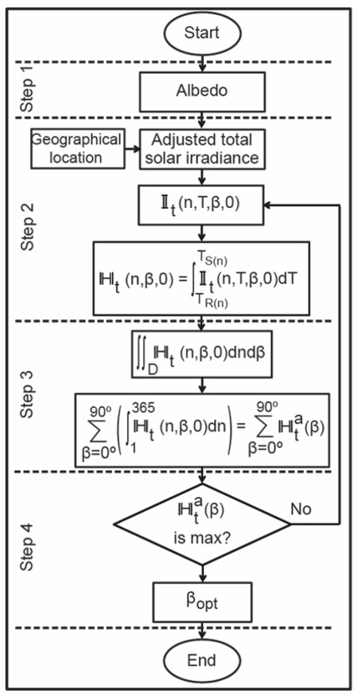
Most authors use the same procedure to calculate the total solar irradiance ($I_t$) on a tilted surface. The procedure in obtaining its components separately: the beam ($I_{bt}$), the diffuse ($I_{dt}$), and the ground reflected ($I_{rt}$) irradiances. These components are defined in [17], and its calculation requires estimating beforehand the beam and the diffuse irradiance on a horizontal plane.

The amount of beam irradiance on a tilted surface can be estimated from the geometric relation between the horizontal plane and the tilted surface [17], which is expressed as:

$$I_{bt}(n,T,\beta ,\gamma )=I_{bh}\left(n,T\right)·\frac{\cos {\theta }_i}{\cos {\theta }_z}$$

(1)

where $I_{bh}$ (W/m${}^2$) is the beam irradiance on a horizontal plane, ${\theta }_z$ ($°$) is the zenith angle of the sun, ${\theta }_i$ ($°$) is the incident angle on a tilted surface, $\beta$ ($°$) is the tilt angle, $\gamma$ ($°$) is the azimuth angle, n (day) is the day of the year and T (h) is the solar time. The incident angle ${\theta }_i$ can be determined following [17].

The diffuse irradiance on a tilted surface has three components: isotropic, circumsolar, and horizon brightening irradiances [17]. Depending on the components considered for calculation, two models may be used: isotropic and anisotropic model. Liu and Jordan’s model [37] is an isotropic model widely used in the specialized literature [38,39]. In the comparison between the isotropic and anisotropic models presented by Mehleri et al. [40], it is concluded that Liu and Jordan’s model obtains accurate results. According to this model, the diffuse irradiance on a tilted surface can be defined as:

$$I_{dt}(n,T,\beta )=I_{dh}\left(n,T\right)·\left(\frac{1+\cos \beta }{2}\right)$$

(2)

where $I_{dh}$(W/m${}^2$) is the diffuse irradiance on a horizontal plane, $\beta$ ($°$) is the tilt angle, n (day) is the day of the year and T (h) is the solar time.

Although it is impossible to exactly compute the ground-reflected irradiance due to the many factors contributing to it [41], most works assume that the reflection on the ground of the beam and diffuse solar irradiances is isotropic [17,37,42,43], and they use (3) to compute the ground-reflected irradiance:

$$I_{rt}(n,T,\beta )=\left(I_{bh}\left(n,T\right)+I_{dh}\left(n,T\right)\right)·{\rho }_g·\left(\frac{1-\cos \beta }{2}\right)$$

(3)

where $I_{bh}$ (W/m${}^2$) is the beam irradiance on a horizontal plane, $I_{dh}$ (W/m${}^2$) is the diffuse irradiance on a horizontal plane, $\beta$ ($°$) is the tilt angle, n (day) is the day of the year, T (h) is the solar time, and ${\rho }_g$ (dimensionless) is the ground reflectance or albedo. Typical ${\rho }_g$ values for different ground surfaces have been computed by [44,45,46]. Some of these values are: for weathered concrete ${\rho }_g$ $=0.22$, for dark surfaces of buildings (red brick, dark paints, etc.) ${\rho }_g=0.27$, and for light surfaces of buildings (light brick, light paints, etc.) ${\rho }_g=0.60$. A value of $0.2$ is commonly adopted if no information is available about ground surface [47].

So, the total solar irradiance on a tilted surface can be calculated as:

$${\mathbb{I}}_t(n,T,\beta ,\gamma )={\mathbb{I}}_{bt}\left(n,T,\beta ,\gamma \right)+{\mathbb{I}}_{dt}\left(n,T,\beta \right)+{\mathbb{I}}_{rt}\left(n,T,\beta \right)$$

(4)

Equation (4) is fitted to each location and climate data and, therefore, fitted under real weather conditions.

In order to compute the adjusted total solar irradiation on a tilted surface for each day of the year, the ordinary method of adjusted solar irradiance integration between sunrise and sunset can be expressed as [2]:

$${\mathbb{H}}_t\left(n,\beta ,\gamma \right)={\int }_{T_R\left(n\right)}^{T_S\left(n\right)}{\mathbb{I}}_t(n,T,\beta ,\gamma )dT$$

(5)

where ${\mathbb{H}}_t$ (Wh/m${}^2$) is the adjusted total solar irradiation on a tilted surface, ${\mathbb{I}}_t$ (W/m${}^2$) is the adjusted hourly distribution of total solar irradiance on a tilted surface, $\beta$ ($°$) is the tilt angle, $\gamma$.($°$) is the azimuth angle, n (day) is the day of the year, T (h) is the solar time, $T_R$ (h) is the sunrise solar time, and $T_S$ (h) is the sunset solar time.

The adjusted annual solar irradiation on a tilted surface, ${\mathbb{H}}_t^a\left(\beta ,\gamma \right)$, for different values of tilt and azimuth angles can be expressed as [2]:

$${\mathbb{H}}_t^a\left(\beta ,\gamma \right)=\sum _{n=1}^{365}{\mathbb{H}}_t\left(n,\beta ,\gamma \right)$$

(6)

The ideal position of a $PV$ module is defined by the optimum tilt and azimuth angles. As it is well known, the optimum azimuth angle is $0°$ in the northern hemisphere [48,49]. Therefore, Equation (5) can be simplified, obtaining the two-variable function, $H_t\left(n,\beta ,0\right)$. The plot of this function is shown in Figure 3 for Madrid (Spanish capital). As the ideal position can be referred to a period of time (year, month, day), $H_t\left(n,\beta ,0\right)$ can be used to obtain the ideal position for a certain period of time.

4. Procedure

The following considerations have been made in this study:

(i)

The effect of the weather conditions for each city under study is taken into account with the method proposed by [31].

(ii)

The Mathematica${}^{\copyright }$ code uses the satellite-derived $PVGIS$ data [50] for each city under study as inputs of monthly-averaged beam and diffuse solar irradiation.

(iii)

Any albedo value can be used.

(iv)

The study was carried out in Spain. However, the procedure can be applied anywhere in the world.

The optimum tilt angle and the total incident energy are outputs of the algorithm.

4.1. Computation of the Optimum Tilt Angle

In what follows, we shall look at several proposals to compute the optimum tilt angle for non-tracker-based panels. Assuming the $PV$ modules are south oriented, the technical literature provides several equations for calculating the annual optimum tilt angle based on the latitude of the site.

4.1.1. Technical Report by the Spanish Institute for the Diversification and Saving of Energy (IDAE)

A Technical Report [51] by IDAE requires that the annual optimum tilt angle be determined by Equation (7):

$${\beta }_{opt}=\lambda -10$$

(7)

where $\lambda$ is the latitude ($°$).

4.1.2. Other Equations

For locations with $\lambda <45°$, Lorenzo [21] proposes the following equation for calculating the annual optimum tilt angle:

$${\beta }_{opt}=3.7+0.69·\left|\lambda \right|$$

(8)

where $\lambda$ is the latitude ($°$). This model is has been used in [52,53].

Jacobson’s model [22] has also been used extensively [23,25,54,55]. This model proposes the following equation for calculating the annual optimum tilt angle:

$${\beta }_{opt}=1.3793+\lambda (1.2011+\lambda (-0.014404+0.000080509\lambda ))$$

(9)

where $\lambda$ is the latitude ($°$).

Equations (7)–(9) do not take into account other variables that influence the annual solar irradiation on a tilted surface, such as albedo.

4.1.3. Cavaleri’s Principle

The previous methods are based on statistical procedures and do not include the effect of albedo variation. In order to take into account the effect of albedo in the determination of the optimum tilt angle, we present an application of Cavaleri’s principle.

Another procedure to obtain the optimum tilt angle is based on maximizing the solar irradiation falling on a tilted surface over a period of time. In this case, the period of time is a year. For this purpose, Cavaleri’s principle can be applied [2,34].

The volume underneath the graph of the equation $H_t\left(n,\beta ,0\right)$ is given by the double integral [2]:

$${\int \int }_D{\mathbb{H}}_t\left(n,\beta ,0\right)dnd\beta$$

(10)

where D is the rectangle $D:[1,365]\times [0,90]$. The application of integral calculus to Cavaleri’s principle yields [2]:

$${\int \int }_D{\mathbb{H}}_t\left(n,\beta ,0\right)dnd\beta =\sum _{\beta =0}^{90}{\int }_1^{365}{\mathbb{H}}_t\left(n,\beta ,0\right)dn=\sum _{\beta =0}^{90}{\mathbb{H}}_t^a\left(\beta \right)$$

(11)

The interval $[0,90]$ can be discretized as the integral for each of the values calculated.

This optimization procedure seeks ${\beta }_{opt}^y$ such that [2]:

$$\underset{\beta }{\max }{\mathbb{H}}_t^a\left(\beta \right)$$

(12)

A flowchart outlining the proposed methodology is shown in Figure 4.

Figure 5 shows the representation of optimum tilt angle in Madrid for each value of ${\rho }_g$. This graph shows that the annual optimum tilt angle is higher as the albedo increases.

This procedure can be used in other parts of the world, both in the northern and southern hemispheres. The proposed procedure is not limited by the latitude of the site. Take for example Cairo, Egypt (Latitude: $30°{29}^{\prime }{24}^{″}$ N, Longitude: $31°{14}^{\prime }{38}^{″}$ W, Altitude: 41 (m)). Figure 6 shows the representation of optimum tilt angle in Cairo for each value of ${\rho }_g$.

4.2. Energy Harvesting

Relative energy harvesting ($REH$) can be used in the evaluation of the equation for the determination of the optimum tilt angle [24]. In this context, it is reasonable to introduce the ”maximum” value of the study, assuming the $PV$ modules are south oriented. For this purpose, we provide a baseline “maximum” value using single-axis trackers aligned to the east–west axis. Duffie’s [17] formula for this tracker is used, which yields:

$$\beta =\arctan \left(\tan {\theta }_z\right|\cos {\gamma }_s\left|\right)$$

(13)

where, in this case, the azimuth angle of the surface depends on ${\gamma }_S$ as follows [17]:

$$\gamma =\left\{\begin{array}{ccc}0°\hfill & \mathrm{if}\hfill & \left|{\gamma }_S\right|<90°\\ 180°\hfill & \mathrm{if}\hfill & \left|{\gamma }_S\right|\ge 90°\end{array}\right.$$

(14)

Table 3. Maximum annual irradiation (MWh/m${}^2$) on a tilted plane.

Id	City	${\mathit{\rho }}_{\mathit{g}}=0.2$	${\mathit{\rho }}_{\mathit{g}}=0.4$	${\mathit{\rho }}_{\mathit{g}}=0.6$	${\mathit{\rho }}_{\mathit{g}}=0.8$
1	Cadiz	2.1835	2.2160	2.2485	2.2810
2	Malaga	2.1413	2.1735	2.2056	2.2378
3	Almeria	2.1996	2.2327	2.2659	2.2990
4	Granada	2.1746	2.2076	2.2407	2.2737
5	Huelva	2.1807	2.2135	2.2464	2.2792
6	Sevilla	2.1798	2.2129	2.2460	2.2791
7	Jaen	2.1125	2.1448	2.1771	2.2094
8	Cordoba	2.1468	2.1797	2.2125	2.2454
9	Murcia	2.0915	2.1244	2.1572	2.1901
10	Alicante	2.0791	2.1116	2.1441	2.1766
11	Badajoz	2.0697	2.1022	2.1347	2.1672
12	Ciudad Real	2.0931	2.1262	2.1593	2.1923
13	Albacete	2.0819	2.1151	2.1483	2.1815
14	Valencia	2.0813	2.1146	2.1480	2.1813
15	Caceres	2.0774	2.1104	2.1434	2.1764
16	Toledo	2.1014	2.1353	2.1693	2.2032
17	Castellon	2.0247	2.0577	2.0907	2.1237
18	Cuenca	2.0284	2.0614	2.0945	2.1275
19	Teruel	1.9784	2.0113	2.0443	2.0773
20	Madrid	2.0861	2.1200	2.1539	2.1878
21	Guadalajara	2.0297	2.0630	2.0963	2.1295
22	Avila	1.9211	1.9529	1.9847	2.0165
23	Segovia	1.7974	1.8272	1.8571	1.8869
24	Salamanca	1.9174	1.9488	1.9802	2.0116
25	Tarragona	2.0053	2.0389	2.0725	2.1061
26	Barcelona	1.9340	1.9655	1.9970	2.0285
27	Zamora	1.9764	2.0094	2.0424	2.0753
28	Lleida	2.0381	2.0723	2.1064	2.1405
29	Zaragoza	2.0400	2.0742	2.1084	2.1427
30	Valladolid	1.9534	1.9862	2.0191	2.0519
31	Soria	1.8812	1.9137	1.9462	1.9787
32	Girona	1.8900	1.9230	1.9561	1.9891
33	Palencia	1.9291	1.9619	1.9946	2.0274
34	Huesca	2.0624	2.09744	2.1324	2.1674
35	Ourense	1.6929	1.7225	1.7521	1.7817
36	Burgos	1.8359	1.8674	1.8988	1.9303
37	Pontevedra	1.6927	1.7221	1.7516	1.7811
38	Logroño	1.7516	1.7825	1.8134	1.8443
39	Leon	1.9185	1.9514	1.9843	2.0171
40	Pamplona	1.6839	1.7140	1.7440	1.7740
41	Vitoria	1.5168	1.5442	1.5717	1.5991
42	Lugo	1.5733	1.6018	1.6304	1.6589
43	Bilbao	1.4052	1.4316	1.4579	1.4843
44	San Sebastian	1.4011	1.4276	1.4541	1.4806
45	Oviedo	1.4549	1.4829	1.5109	1.5388
46	A Coruña	1.5356	1.5640	1.5924	1.6208
47	Santander	1–4541	1.4814	1.5088	1.5361

shows the maximum annual irradiation for single-axis trackers aligned to the east–west axis for each value of ${\rho }_g$. These are maximum values which obtain a tilted surface assuming the $PV$ modules are south oriented.

$REH$ is then calculated as the difference between the energy harvested according to each specific model under study and the single-axis trackers aligned with the east–west axis, as a $percentage$ of energy:

$$RE{H}_1=\frac{H_{\ast }-H_{1-axis}}{H_{1-axis}}·100$$

(15)

where the subindex ∗ stands, as above, for the corresponding equation ($IDAE$ recommendation, Lorenzo’s, or Jacobson’s equations).

The $REH$ can be also calculated as the difference between the energy harvested after application of the model under study and the method based maximizing the total irradiation incident on a tilted surface applying Cavaleri’s principle, as a $percentage$ of energy:

$$RE{H}_2=\frac{H_{\ast }-H_{Cavaleri}}{H_{Cavaleri}}·100$$

(16)

where the subindex ∗ stands, as above, for the corresponding equation ($IDAE$ recommendation, Lorenzo’s equation, Jacobson’s equation).

Based on (15) and (16), one can obtain reliable information regarding the model from a practical point of view. In addition, these equations will allow us to evaluate the validity of the models when the albedo is different from the usual.

5. Results and Discussion

Equations (8) and (9) are widely used to estimate the amount of total irradiation on a tilted plane. Equation (7) is recommended by a technical report by $IDAE$. The aim of this section is to assess these equations depending on the albedo variations. Based on the equations presented in Section 2, each type of solar irradiance is calculated with the effect of the weather conditions. A Mathematica${}^{\copyright }$ optimization code was used for computing the direct, diffuse, and reflected components of the solar irradiance. The satellite-derived $PVGIS$ data [50] were used to obtain the monthly-averaged beam and diffuse solar irradiation of each city under study. The method proposed by [31] was used to account for the effect of weather conditions.

5.1. Equations as Function of Latitude

We compare the yearly solar irradiation using the models in (7)–(9) to determine the optimum tilt angle, taking as a baseline the single-axis tracker. Figure 7 shows a graphical representation of the yearly $RE{H}_1$ between the use of the annual optimum tilt angle and a single-axis tracker for each value of ${\rho }_g$ for which Equation (15) has been used. The charts show the loss of harvested solar energy with respect to the baseline for four different albedo values.

The following conclusions can be inferred:

(i)

The annual solar irradiation for each city is consistently higher as the albedo increases.

(ii)

For ${\rho }_g=0.2$, the three models closely match. Lorenzo’s and Jacobson’s equations obtain very similar total annual irradiation values. The maximum $REH$ of total yearly irradiation is $-6.76\%$ in the case of $IDAE$’s guidelines, $-6.66\%$ for Lorenzo’s equation, and $-6.65\%$ for Jacobson’s equation. The deviations are not greater than $0.11\%$. The reflectivity of most types of ground surfaces is rather low; therefore, the contribution of this type of solar irradiance falling on a $PV$ module is low. When no specific albedo values are available, the value of $0.2$ is typically assumed [47]. Therefore, in this case, these equations are valid.

(iii)

For ${\rho }_g=0.4$, Lorenzo’s equation and Jacobson’s equation still obtain very similar total annual irradiation values. However, the $IDAE$ recommendation begins to worsen its results. The maximum $REH$ of total annual irradiation is $-7.25\%$ for $IDAE$ guideline, $-7.00\%$ for Lorenzo’s equation, and $-6.93\%$ for Jacobson’s equation.

(iv)

For ${\rho }_g=0.6$, the $IDAE$ recommendation worsens its results by $1\%$ compared with ${\rho }_g=0.2$, and Lorenzo’s equation and Jacobson’s equation in $0.6\%$. The maximum $REH$ of total annual irradiation is $-7.73\%$ for $IDAE$ guideline, $-7.33\%$ for Lorenzo’s equation, and $-7.20\%$ for Jacobson’s equation.

(v)

For ${\rho }_g=0.8$, Lorenzo’s equation and Jacobson’s equation still obtain very similar total annual irradiation values, but their results are worsened by $1\%$ compared with ${\rho }_g=0.2$. $IDAE$ recommendation obtains the worst results. The maximum $REH$ of total annual irradiation is $-8.19\%$ for the $IDAE$ guidelines, $-7.66\%$ for Lorenzo’s equation, and $-7.46\%$ for Jacobson’s equation.

(vi)

The reason for the small difference between the results obtained by using Lorenzo’s equation and Jacobson’s equation is that they are based on the same procedure. For locations with $\lambda \le 40.7°$, Jacobson’s equation yields better results. For $\lambda \ge 41.4°$, Lorenzo’s equation obtains better results. For $40.7°<\lambda <41.4°$, both equations produce the same results.

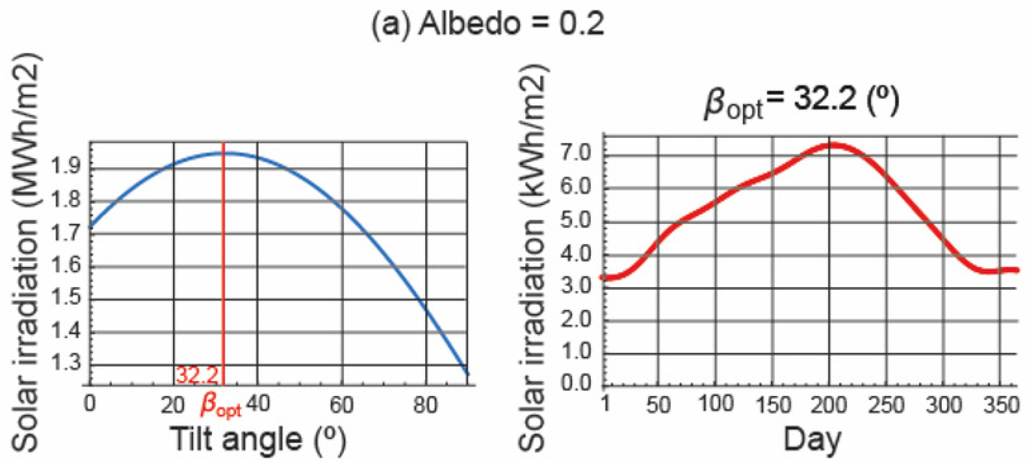
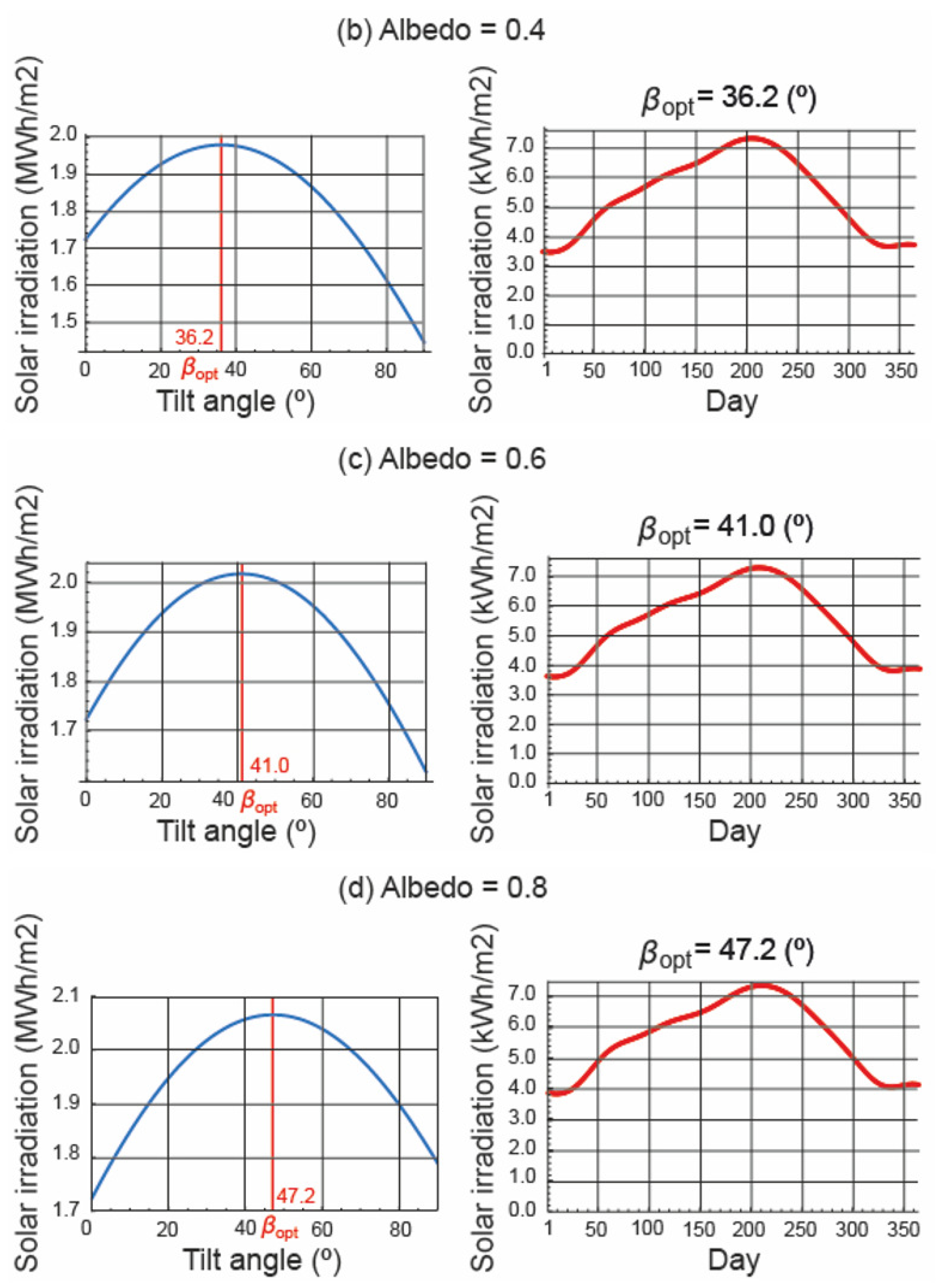
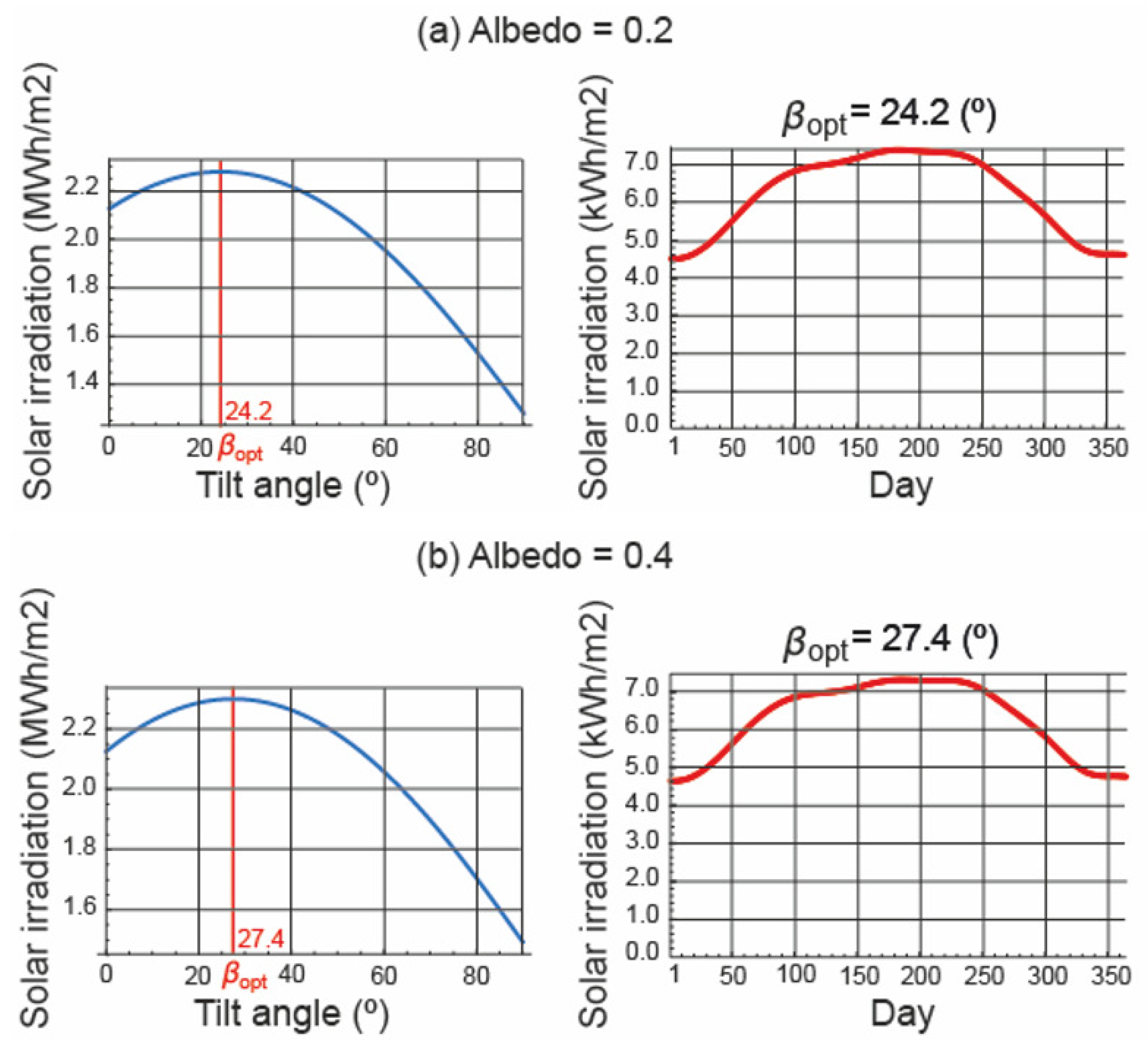
5.2. Method Based on to Maximize the Total Irradiation Incident on a Tilted Surface

Equations (7)–(9) depend on latitude but not on albedo. In contrast, the procedure that maximizes the total irradiation incident on a tilted surface takes into account the albedo. Figure 8 shows the influence of albedo on the annual optimum tilt angle in Madrid. The annual optimum tilt angle is higher as albedo increases.

The equations to determine the optimum tilt angle for Spain are compared with the method based on maximizing the total irradiation incident on a tilted surface applying Cavaleri’s principle. Figure 9 shows a graphical representation of the yearly $RE{H}_2$ comparing the use of different equations to determine the optimum tilt angle and the application of the Cavaleri’s principle for each value of ${\rho }_g$, for which (16) was used.

Figure 9 suggests the following conclusions:

(i)

The method that maximizes the total irradiation incident on a tilted surface obtains the best results.

(ii)

For ${\rho }_g=0.2$, the three equations closely match with the method that maximizes the total irradiation incident on a tilted surface.

(iii)

For ${\rho }_g=0.4$, Lorenzo’s equation and Jacobson’s equation continue to give very similar values for total annual irradiation. However, the $IDAE$ recommendation begins to worsen its results. The maximum $REH$ of total annual irradiation is $-0.55\%$ for the $IDAE$ guideline, $-0.36\%$ for Lorenzo’s equation, and $-0.40\%$ for Jacobson’s equation.

(iv)

For ${\rho }_g=0.6$, the $IDAE$ recommendation worsens its results by $1.2\%$ compared with ${\rho }_g=0.2$, and Lorenzo’s equation and Jacobson’s equation worsen by $0.7\%$. The maximum $REH$ of total annual irradiation is $-1.34\%$ for the $IDAE$ guideline, $-0.95\%$ for Lorenzo’s equation, and $-1.10\%$ for Jacobson’s equation.

(v)

For ${\rho }_g=0.8$, Lorenzo’s equation and Jacobson’s equation still obtain very similar total annual irradiation values, but their results are worsened by $2.0\%$ compared with ${\rho }_g=0.2$. The $IDAE$ recommendation obtains the worst results. The maximum $REH$ of total annual irradiation is $-2.62\%$ for the $IDAE$ guideline, $-2.38\%$ for Lorenzo’s equation, and $-2.46\%$ for Jacobson’s equation.

(vi)

The greater the albedo, the greater the error introduced by the three models, since they only account for the latitude of the place. The results suggest that the proposed optimization method is able to take into account the variation of the albedo.

(vii)

With increased albedo, the $IDAE$ guideline obtains the worst results

(viii)

It is recommended to use Lorenzo’s equation and Jacobson’s equation for the cities studied for ${\rho }_g=0.2$.

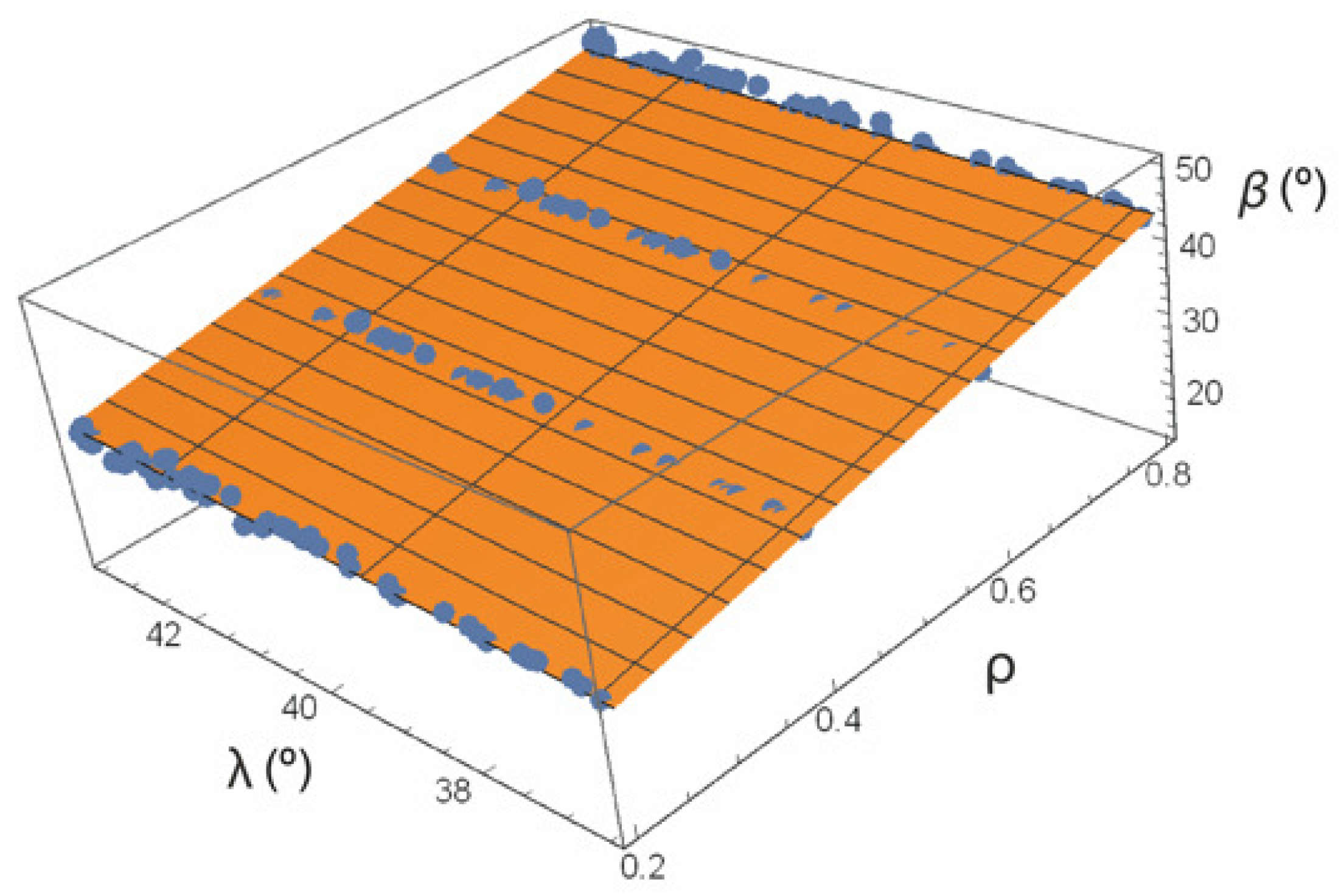
5.3. Simplified Model for the Annual Optimum Tilt Angle

Previous studies have clearly shown the need to take into account the influence of albedo when calculating the optimum tilt angle. The method based on Cavaleri’s principle presents a high accuracy in the calculations, as it takes into account not only the albedo but also the direct and diffuse irradiance regarding the meteorological conditions of each location. However, we are aware that their use requires the use of software that may not be available to all users. Therefore, in this section, we present a simplified model (similar to Lorenzo’s or Jacobson’s) that produces good approximation to the value of the optimum annual tilt obtained with our method.

We proceeded with a Monte Carlo-like experiment, using the latitude and altitude data of the 47 cities—as well as $four$ cases of varying albedo—as samples. After applying Cavalieri’s principle to these samples, we obtained the optimum tilt, which we employed as our response variable in a regression problem, in which the regressors or independent variables were precisely the latitude, altitude, and albedo. We then proceeded with a symbolic regression through genetic programming based on Python’s project gplearn [56]. Symbolic regression is a machine learning technique employed to identify underlying mathematical expressions based on a catalog of possible functions. It begins by constructing a population of naive random formulae to represent a relationship between regressors and a response variable in order to predict new data. Each successive generation of programs then evolves from the previous one by selecting the fittest individuals from the population to undergo genetic operations. Genetic programming represents solutions to the regression problem as trees (by contrast, genetic algorithms represent them as strings). Using this tree representation is quite convenient in our application, since mathematical expressions can be represented by trees.

We performed a symbolic regression analysis by testing arithmetic functions along with trigonometrical and power functions as possible fittings. After ten thousand iterations, the best parsimonious fit turned out to be a simple linear regression model. We comment on two alternatives next.

(i) A first linear model, a function of latitude $\lambda$ and albedo $\rho$, is:

$$\beta (\lambda ,\rho )=7.91039+0.437359\lambda +25.6234\rho$$

(17)

The goodness of fit obtained, as measured by the coefficient of determination, gives a value of $R^2=0.9537.$ In Figure 10. we see the cloud of $4\times 47=188$ sample points and the fitting surface (the plane in this case) $\beta (\lambda ,\rho ).$

(ii) A second model, incorporating altitude A, is:

$$\beta (\lambda ,A,\rho )=7.48917-0.000659558A+0.454052\lambda +25.6234\rho$$

(18)

The goodness of fit is very similar to the previous one, obtaining now $R^2=0.9553$. A noteworthy feature is that the albedo term is the same in both models. The altitude of the location only plays a marginal role in accuracy.

After extensive testing, we have found that it does not pay to use higher degree models (quadratic or cubic), as they unnecessarily complicate the model with little improvement in goodness of fit. For example, the quadratic model and the cubic model we obtain are:

$$\beta (\lambda ,\rho )=-110.245+6.48852\lambda -0.0753977{\lambda }^2+11.0489\rho +14.5745{\rho }^2$$

(19)

$$\begin{array}{c}\beta (\lambda ,\rho )=204.222-17.1264\lambda +0.513803{\lambda }^2-0.00489214{\lambda }^3+\hfill \\ \hfill 14.9574\rho +5.79787{\rho }^2+5.85106{\rho }^3\end{array}$$

(20)

obtaining $R^2=0.9658$ and $R^2=0.9659$, respectively.

We have also investigated the possibility of finding non-linear models for the fit. By way of example, we present two of the models of this type that have given us the best results, combining precision and simplicity. On the one hand, the simplest non-linear model:

$$\beta (\lambda ,\rho )=25.6067+0.634111\lambda \rho$$

(21)

which with the same variables ($\lambda$ and $\rho$) gives an $R^2=0.9541$. On the other hand, we also tested a more sophisticated model that incorporates the ratio between the adjusted annual beam irradiance on a horizontal plane, ${\mathbb{I}}_{bh}^a$ (kWh/m${}^2$) and the adjusted annual diffuse irradiance on a horizontal plane ${\mathbb{I}}_{dh}^a$ (kWh/m${}^2$). In this case, we obtained as the best fit:

$$\beta (\lambda ,\rho ,{\mathbb{I}}_{bh}^a,{\mathbb{I}}_{dh}^a)=-9.64449+0.769701\lambda +25.6234\rho +2.1472\frac{{\mathbb{I}}_{bh}^a}{{\mathbb{I}}_{dh}^a}$$

(22)

and the goodness of fit is very similar, now obtaining $R^2=0.9596$.

To deepen this analysis, the key factor is to study the seasonality of the irradiances of each location. The study is very complex and again does not produce a substantial improvement of the fit.

6. Conclusions

In this paper, the optimum tilt angles of photovoltaic systems for urban applications have been analysed for 47 cities in Spain through a Mathematica${}^{\copyright }$ optimization code. These cities are the Spanish province capitals and represent the most populous cities. The analysis was carried out for fixed tilt angle and different types of albedo, taking into account both the geographical and the meteorological conditions of the sites. The yearly energy harvesting has been evaluated using: (i) models based on latitude ($IDAE$’s guideline, and Lorenzo’s and Jacobson’s models); (ii) equations as function of latitude ($IDAE$ guideline, Lorenzo’s equation, Jacobson’s equation) versus a method that maximizes the total irradiation incident on a tilted surface. The summary of the results is as follows:

(i)

The use of the equations as a function of latitude increases the annual $REH$ by increasing the albedo. When the albedo was $0.2$, the annual $REH$ was very similar for all three equations. Lorenzo’s and Jacobson’s models did not appreciably change the annual $REH$ in the range of albedos studied.

(ii)

With regard to single-axis tracker, the minimum and maximum value of the percentage of $REH$ per year obtained were $6.76$ (${\rho }_g=0.2$) and $8.19\%$ (${\rho }_g=0.8$) for $IDAE$’s guideline, $6.66$ (${\rho }_g=0.2$) and $7.66\%$ (${\rho }_g=0.8$) for Lorenzo’s model, $6.65\%$ (${\rho }_g=0.2$) and $7.46\%$ (${\rho }_g=0.8$) for Jacobson’s model.

(iii)

The annual $REH$ was increased when the equations as a function of latitude were used, compared with the method that maximizes the total irradiation incident on a tilted surface. This increase is stronger for albedo values equal to $0.8$.

(iv)

The yearly optimum tilt angle is higher as albedo increases. Therefore, equations that only depend on latitude are less accurate as the albedo increases. With regard to the method that maximizes the total irradiation incident on a tilted surface, the minimum and maximum value of the percentage of $REH$ per year obtained were $0.01$ and $2.62\%$ for $IDAE$ guideline, $0.00$ and $2.38\%$ for Lorenzo’s equation, and $0.00\%$ and $2.46\%$ for Jacobson’s equation.

(v)

We have obtained two linear models that account for the latitude, albedo and the altitude of the location to predict the optimum tilt angle. We believe that these formulae show great simplicity of use with acceptable accuracy.

We believe that our methodology can be used to make optimal decisions in the choice of tilt angle in photovoltaic modules as a function of albedo, obtaining important benefits from the point of view of total energy absorption. Future work will consist of an experimental study of the effect of albedo on the equations used in the determination of the optimum tilt angle.

References

1. United Nations. Doha Amendment to the Kyoto Protocol; Adopted, Decision 1/CMP; C.N.718.2012.TREATIES-XXVII.7.c; United Nations: Rome, Italy, 2012; Volume 8. [Google Scholar]
2. Barbón, A.; Ayuso, P.F.; Bayxoxn, L.; Silva, C.A. A comparative study between racking systems for photovoltaic power systems. Renew. Energy 2021, 180, 424–437. [Google Scholar] [CrossRef]
3. Ghodbane, M.; Boumeddane, B.; Said, Z.; Bellos, E. A numerical simulation of a linear Fresnel solar reflector directed to produce steam for the power plant. J. Clean. Prod. 2019, 231, 494–508. [Google Scholar] [CrossRef]
4. Byrne, J.; Hughes, K.; Toly, N.; Wang, Y.-D. Can cities sustain life in the greenhouse? Bull. Sci. Technol. Soc. 2006, 26, 84–95. [Google Scholar] [CrossRef]
5. In Focus: Energy Efficiency in Buildings. Available online: https://ec.europa.eu/info/news/focus-energy-efficiency-buildings-2020-feb-17_en (accessed on 23 July 2022).
6. Economidou, M.; Todeschi, V.; Bertoldi, P.; D’Agostino, D.; Zangheri, P.; Castellazzi, L. Review of 50 years of EU energy efficiency policies for buildings. Energy Build. 2020, 225, 110322. [Google Scholar] [CrossRef]
7. Gulkowski, S. Specific Yield Analysis of the Rooftop PV Systems Located in South-Eastern Poland. Energies 2022, 15, 3666. [Google Scholar] [CrossRef]
8. Child, M.; Kemfert, C.; Bogdanov, D.; Breyer, C. Flexible electricity generation, grid exchange and storage for the transition to a 100% renewable energy system in Europe. Renew. Energy 2019, 139, 80–101. [Google Scholar] [CrossRef]
9. Gómez-Navarro, T.; Brazzini, T.; Alfonso-Solar, D.; Vargas-Salgado, C. Analysis of the potential for PV rooftop prosumer production: Technical, economic and environmental assessment for the city of Valencia (Spain). Renew. Energy 2021, 174, 372–381. [Google Scholar] [CrossRef]
10. Jacobson, M.Z.; Delucchi, M.A.; Bauer, Z.A.F.; Goodman, S.C.; Chapman, W.E.; Cameron, M.A.; Bozonnat, C.; Chobadi, L.; Clonts, H.A.; Enevoldsen, P.; et al. 100% clean and renewable wind, water, and sunlight (WWS) all-sector energy roadmaps for 139 countries of the world. Joule 2017, 1, 108–121. [Google Scholar] [CrossRef] [Green Version]
11. Buonocore, J.J.; Luckow, P.; Norris, G.; Spengler, J.D.; Biewald, B.; Fisher, J.; Levy, J.I. Health and climate benefits of different energy-efficiency and renewable energy choices. Nat. Clim. Chang. 2016, 6, 100–105. [Google Scholar] [CrossRef]
12. Peng, J.; Lu, L. Investigation on the development potential of rooftop PV system in Hong Kong and its environmental benefits. Renew. Sustain. Energy Rev. 2013, 27, 149–162. [Google Scholar] [CrossRef]
13. Arcos-Vargasa, A.; Cansino, J.M.; Román-Collado, R. Economic and environmental analysis of a residential PV system: A profitable contribution to the Paris agreement. Renew. Sustain. Energy Rev. 2018, 94, 1024–1035. [Google Scholar] [CrossRef]
14. Jan, I.; Ashfaq, W.U.M. Social acceptability of solar photovoltaic system in Pakistan: Key determinants and policy implications. J. Clean. Prod. 2020, 274, 123140. [Google Scholar] [CrossRef]
15. Assouline, D.; Mohajeri, N.; Scartezzini, J.-L. Quantifying rooftop photovoltaic solar energy potential: A machine learning approach. Sol. Energy 2017, 141, 278–296. [Google Scholar] [CrossRef]
16. Ordóñez, J.; Jadraque, E.; Alegre, J.; Martínez, G. Analysis of the photovoltaic solar energy capacity of residential rooftops in Andalusia (Spain). Renew. Sustain. Energy Rev. 2010, 14, 2122–2130. [Google Scholar] [CrossRef]
17. Duffie, J.A.; Beckman, W.A. Solar Engineering of Thermal Processes, 4th ed.; John Wiley & Sons: New York, NY, USA, 2013. [Google Scholar]
18. Raptis, I.-P.; Moustaka, A.; Kosmopoulos, P.; Kazadzis, S. Selecting Surface Inclination for Maximum Solar Power. Energies 2022, 13, 4784. [Google Scholar] [CrossRef]
19. Barbón, A.; Ghodbane, M.; Bayxoxn, L.; Said, Z. A general algorithm for the optimization of photovoltaic modules layout on irregular rooftop shapes. J. Clean. Prod. 2022, 365, 132774. [Google Scholar] [CrossRef]
20. Ullah, A.; Imran, H.; Maqsood, Z.; Butt, N.Z. Investigation of optimal tilt angles and effects of soiling on PV energy production in Pakistan. Renew. Energy 2019, 139, 830–843. [Google Scholar] [CrossRef]
21. Lorenzo, E. Energy collected and delivered by PV modules. In Handbook of Photovoltaic Science and Engineering; John Wiley & Sons: Hoboken, NJ, USA, 2011; pp. 984–1042. [Google Scholar]
22. Jacobson, M.Z.; Jadhav, V. World estimates of PV optimal tilt angles and ratios of sunlight incident upon tilted and tracked PV panels relative to horizontal panels. Sol. Energy 2018, 169, 55–66. [Google Scholar] [CrossRef]
23. Nicolás-Martín, C.; Santos-Martín, D.; Chinchilla-Sxaxnchez, M.; Lemon, S. A global annual optimum tilt angle model for photovoltaic generation to use in the absence of local meteorological data. Renew. Energy 2020, 161, 722–735. [Google Scholar] [CrossRef]
24. Soulayman, S.; Hammoud, M. Optimum tilt angle of solar collectors for building applications in mid-latitude zone. Energy Convers. Manag. 2016, 124, 20–28. [Google Scholar] [CrossRef]
25. Al Garni, H.Z.; Awasthi, A.; Wright, D. Optimal orientation angles for maximizing energy yield for solar PV in Saudi Arabia. Renew. Energy 2019, 133, 538–550. [Google Scholar] [CrossRef]
26. SOLARGIS. Available online: https://solargis.com/maps-and-gis-data/download/world (accessed on 9 July 2021).
27. Danandeh, M.A.; Mousavi, S.M. Solar irradiance estimation models and optimum tilt angle approaches: A comparative study. Renew. Sustain. Energy Rev. 2018, 92, 319–330. [Google Scholar] [CrossRef]
28. Antonanzas-Torres, F.; Urraca, R.; Polo, J.; Perpi nán-Lamigueiro, O.; Escobar, R. Clear sky solar irradiance models: A review of seventy models. Renew. Sustain. Energy Rev. 2019, 107, 374–387. [Google Scholar] [CrossRef]
29. Salazar, G.; Gueymard, C.; Galdino, J.B.; Castro Vilela, O. Solar irradiance time series derived from high-quality measurements, satellite-based models, and reanalyses at a near-equatorial site in Brazil. Renew. Sustain. Energy Rev. 2020, 117, 109478. [Google Scholar] [CrossRef]
30. Fan, J.; Chen, B.; Wu, L.; Zhang, F.; Lu, X. Evaluation and development of temperature-based empirical models for estimating daily global solar radiation in humid regions. Energy 2018, 144, 903–914. [Google Scholar] [CrossRef]
31. Barbón, A.; Ayuso, P.F.; Bayxoxn, L.; Fernández-Rubiera, J.A. Predicting beam and diffuse horizontal irradiance using Fourier expansions. Renew. Energy 2020, 154, 46–57. [Google Scholar] [CrossRef]
32. Hottel, H.C. A simple model for estimating the transmittance of direct solar radiation through clear atmosphere. Sol. Energy 1976, 18, 129–134. [Google Scholar] [CrossRef]
33. Liu, B.Y.H.; Jordan, R.C. The interrelationship and characteristic distribution of direct, diffuse and total solar radiation. Sol. Energy 1960, 4, 1–19. [Google Scholar] [CrossRef]
34. Barbón, A.; Bayxoxn-Cueli, C.; Bayxoxn, L.; Rodríguez-Suanzes, C. Analysis of the tilt and azimuth angles of photovoltaic systems in non-ideal positions for urban applications. Appl. Energy 2022, 305, 117802. [Google Scholar] [CrossRef]
35. Barbón, A.; Fernández-Rubiera, J.A.; Martínez-Valledor, L.; Pérez-Fernxaxndez, A.; Bayxoxn, L. Design and construction of a solar tracking system for small-scale linear Fresnel reflector with three movements. Appl. Energy 2021, 285, 116477. [Google Scholar] [CrossRef]
36. WRDC. World Radiation Data Centre. 2021. Available online: http://wrdc.mgo.rssi.ru/ (accessed on 9 July 2021).
37. Liu, B.Y.H.; Jordan, R.C. The long-term average performance of flat-plate solar energy collectors. Sol. Energy 1963, 7, 53–74. [Google Scholar] [CrossRef]
38. Bertrand, C.; Housmans, C.; Leloux, J.; Journée, M. Solar irradiation from the energy production of residential PV systems. Renew. Energy 2018, 125, 306–318. [Google Scholar] [CrossRef]
39. Okoye, C.O.; Solyalı, O. Optimal sizing of stand-alone photovoltaic systems in residential buildings. Energy 2017, 126, 573–584. [Google Scholar] [CrossRef]
40. Mehleri, E.D.; Zervas, P.L.; Sarimveis, H.; Palyvos, J.A.; Markatos, N.C. Determination of the optimal tilt angle and orientation for solar photovoltaic arrays. Renew. Energy 2010, 35, 2468–2475. [Google Scholar] [CrossRef]
41. Coakley, J.A. Reflectance and albedo, surface. In Encyclopedia of the Atmosphere; Academic Press: Washington, DC, USA, 2003; pp. 1914–1923. [Google Scholar]
42. Mamun, M.A.A.; Islam, M.M.; Hasanuzzaman, M.; Selvaraj, J. Effect of tilt angle on the performance and electrical parameters of a PV module: Comparative indoor and outdoor experimental investigation. Energy Built Environ. 2022, 3, 278–290. [Google Scholar] [CrossRef]
43. Yadav, S.; Panda, S.K.; Tripathy, M. Performance of building integrated photovoltaic thermal system with PV module installed at optimum tilt angle and influenced by shadow. Renew. Energy 2018, 127, 11–23. [Google Scholar] [CrossRef]
44. Muneer, T. Solar Radiation and Day Light Models, 1st ed.; Elsevier: Oxford, UK, 2004. [Google Scholar]
45. Dobos, E. Albedo. In Encyclopedia of Soil Science; CRC Press: Boca Raton, FL, USA, 2006; Volume 2, pp. 24–25. [Google Scholar]
46. Weihs, P.; Mursch-Radlgruber, E.; Hasel, S.; Gützer, C.; Brandmaier, M.; Plaikner, M. Investigation of the effect of sealed surfaces on local climate and thermal stress. In EGU General Assembly Conference Abstracts; Geophysical Research Abstracts: Vienna, Austria, 2015; p. 12616. [Google Scholar]
47. Pérez-Gallardo, J.R.; Azzaro-Pantel, C.; Astier, S.; Domenech, S.; Aguilar-Lasserre, A. Ecodesign of photovoltaic grid-connected systems. Renew. Energy 2014, 64, 82–97. [Google Scholar] [CrossRef] [Green Version]
48. Chinchilla, M.; Santos-Martín, D.; Carpintero-Rentería, M.; Lemon, S. Worldwide annual optimum tilt angle model for solar collectors and photovoltaic systems in the absence of site meteorological data. Appl. Energy 2021, 281, 116056. [Google Scholar] [CrossRef]
49. Lv, Y.; Si, P.; Rong, X.; Yan, J.; Feng, Y.; Zhu, X. Determination of optimum tilt angle and orientation for solar collectors based on effective solar heat collection. Appl. Energy 2018, 219, 11–19. [Google Scholar] [CrossRef]
50. PVGIS, Joint Research Centre (JRC). 2019. Available online: http://re.jrc.ec.europa.eu/pvg_tools/en/tools.html#PVP (accessed on 9 July 2022).
51. IDAE. Technical Conditions for PV Installations Connected to the Grid. Report Available from the Publication Services of the Institute for Diversification and Energy Savings, Spain. Available online: http://www.idae.es (accessed on 10 September 2022). (In Spanish).
52. Marzo, A.; Ferrada, P.; Beiza, F.; Besson, P.; Alonso-Montesinos, J.; Ballestrín, J.; Román, R.; Portillo, C.; Escobar, R.; Fuentealba, E. Standard or local solar spectrum? Implications for solar technologiesstudies in the Atacama desert. Renew. Energy 2018, 127, 871–882. [Google Scholar] [CrossRef]
53. Fernández-Infantes, A.; Contreras, J.; Bernal-Agustín, J.L. Design of grid connected PV systems considering electrical, economical and environmental aspects: A practical case. Renew. Energy 2006, 31, 2042–2062. [Google Scholar] [CrossRef]
54. Ascencio-Vásquez, J.; Brecl, K.; Topič, M. Methodology of Köppen-Geiger-Photovoltaic climate classification and implications to worldwide mapping of PV system performance. Sol. Energy 2019, 191, 672–685. [Google Scholar] [CrossRef]
55. Tröndle, T.; Pfenninger, S.; Lilliestam, J. Home-made or imported: On the possibility for renewable electricity autarky on all scales in Europe. Energy Strategy Rev. 2019, 26, 100388. [Google Scholar] [CrossRef]
56. Genetic Programming in Python, with a Scikit-Learn Inspired and Compatible API. 2021. Available online: https://github.com/trevorstephens/gplearn (accessed on 9 July 2022).
Figure 1. Map showing locations of cities used.
Energies 15 07905 g001
Figure 2. Global irradiance map for horizontal surface in Spain [26].
Energies 15 07905 g002
Figure 3. Adjusted total solar irradiation on a tilted surface H t n , β , 0 for Madrid.
Energies 15 07905 g003
Figure 4. A flowchart outlining the proposed methodology.
Energies 15 07905 g004
Figure 5. One discretization for H t a ( β ) in Madrid.
Energies 15 07905 g005aEnergies 15 07905 g005b
Figure 6. One discretization for H t a ( β ) in Cairo.
Energies 15 07905 g006aEnergies 15 07905 g006b
Figure 7. Yearly REH between the equations as function of latitude and single-axis tracker.
Energies 15 07905 g007
Figure 8. Plot of H t a ( β ) in Madrid.
Energies 15 07905 g008
Figure 9. Yearly REH between the equations as function of latitude and the method based on maximizing the total irradiation incident on a tilted surface.
Energies 15 07905 g009
Figure 10. Fitting surface β ( λ , ρ ) .
Energies 15 07905 g010