Abstract
Aiming at the problem that the current dynamic economic dispatch (DED) fails to consider the response risk of spinning reserve caused by the fluctuation and uncertainty of wind power, we work out a DED problem considering time-coupling spinning reserve response risk while the stochasticity and variability arising from RESs are taken into consideration. The developed framwork unified the response risk of reserve caused by forced shutdown of the unit into the response risk caused by time coupling. The expected customer interruption cost (ECOST) and the expected abandoned wind cost considering this reserve response risk are added to the objective function. While seeking the minimum objective function, the system is automatically configured with suitable reserve to ensure the consistency of the system’s response risk in each period. An improved multi-universe parallel quantum genetic algorithm was used to solve the model. Numerical examples and analysis prove the effectiveness and feasibility of the proposed method.
1. Introduction
China [1], United States [2], and Europe [3] have, respectively, proposed the goal of achieving 60%, 80%, and 100% of electricity from renewable energy by 2050. Wind power generation, as the most economically promising power generation method among non-water renewable energy sources, is being developed as an alternative energy source to a dominant energy source [4]. However, due to inherent characteristics of fluctuation and uncertainty, the integration of large-scale wind power into the power grid creates a significant impact on the operation and dispatch of the power system [5,6,7,8].
The fluctuation of wind power means that its maximum power output can be changed continuously through time, while the uncertainty means that its maximum output cannot be accurately predicted. The fluctuation characteristic of wind power between different dispatch periods can be handled by adjusting base points of conventional units, while uncertainty and fluctuation of wind power within a single period of time require a certain amount of additional spinning reserve in dispatch. Both of them will further strengthen the coupling of dispatch resources at different time intervals; therefore, compared to static optimal dispatch methods, forward-looking dynamic economic dispatch [9] can be more suitable for power systems with high wind power scales of wind power integration [10,11]. Methods of improving traditional deterministic dynamic economic dispatch to cope with the impact of wind power integration have always been hot topics in academic research [10,11,12,13,14]. However, current research fails to consider carefully the impact of wind power uncertainty and fluctuation on the response risk of spinning reserve, which may easily lead to inconsistent response risk levels, and make dispatch decisions conservative or inevitably aggressive.
In traditional dynamic economic dispatch problems, the response risks of spinning reserve caused by faults of thermal units were mainly considered. Reference [15] proposed that the reserve configuration in dynamic economic dispatch should be able to maintain the response risk of the system at a given level in each period, and gave a heuristic algorithm for dynamic economic dispatch considering the risk of system response. This method decouples the time period through the accumulation variable method. For a single time period after decoupling, an iterative method to evaluate the risk of dispatching and response was utilized and required that the response risk in each time period of the system was maintained at the given level. In [16], the expected customer interruption cost (ECOST) in dispatch was considered in the objective function through the expected energy not supplied (EENS), and optimized the interrupted energy assessment rate (IEAR) to configure appropriate backups. Reference [17] considered the risk of load-loss caused by forced outage of conventional units, and took the risk of spinning reserve under N-1 condition by setting the risk of load-loss into account. In [18], the system reserve capacity was divided into automatic generation control (AGC) capacity and emergency reserve capacity, and considered the system reserve risk under N-1 condition with chance-constraint. However, these studies do not consider the new risk of spinning reserve response led by the integration of wind power.
To cope with fluctuation and uncertainty of wind power, the reserve provided by the power system needs faster response speed, bi-directional regulation capability, and better continuous action capability, which can be called flexibility [19,20]. Grid flexibility has become an essential resource to consider in actual power system dispatch and control. References [21,22] describe a pilot project in Greece that addresses the challenges of congestion and balancing management that system operators face due to high penetration of renewable energy sources. Available resources of the grid’s flexibility are identified and the results suggest that flexibility resources derive through improved predictions; efficient forecasts from numerical weather predictions with greater spatial resolution and integration of artificial intelligence prevent the power system from entering dangerous topological or operational states. The need for flexibility leads to a significant increase in the magnitude and frequency of standby actions. This leads to increased interlocking of standby releases between different time periods, and thus the risk of standby response due to time-period coupling are greatly increased. In current economic dispatch research, this effect is mainly indicated in different measures for power regulation rate constraints of conventional units. In traditional economic dispatch, conventional units dominate the power supply. Correspondingly, the unit regulation rate constraint is utilized from base point to base point due to smaller action amplitudes of the reserve caused by load forecasting errors and the lower probability of accident reserve action. However, with the increase in the penetration rate of renewable energy power generation, on one hand, the dominant position of conventional units is being weaken; on the other hand, the amplitudes and frequencies of reserve actions also continue to rise. The traditional unit regulation rate constraint is no longer applicable. For this purpose, reference [23] uses a flexibility constraint on the unit regulation rate, which requires that the reserve provided by the units can be reversed and completely released in two adjacent periods. Obviously, these constraints are stricter than traditional forms. Additionally, these constraints can ensure that the reserve provided by the units is decoupled between time periods, indicating that the response risk generated by the time-period coupling is zero. These constraints are suitable for a rolling economic dispatch method for which only two time periods are considered, but dynamic economic dispatch methods need to take multiple time periods into consideration, so the risk level set is too harsh and its decisions will be too conservative to ensure the economy. Current dynamic economic dispatch research does not consider how to determine this type of spinning reserve response risk.
Inspired by the aforementioned works, this paper proposes a new dynamic economic dispatch method with high levels of wind power integration. The method presented considers comprehensively the response risks caused by the coupling and containment between different time periods provided by conventional units, together with the response risks caused by forced outage, which ensures the consistency of the response risk level of the system during each time period. This paper takes the expectations of user outage loss and wind curtailment considering the response risks of spinning reserve into account in the objective function. This method pursues a minimum for the objective function and automatically disposes suitable reserve for the system. Owing to a large number of convolution calculations in the optimization process, traditional methods are difficult to solve. This study adopts an improved multi-universe parallel quantum genetic algorithm to improve the speed and convergence of model solution.
The rest of this paper is structured as follows. Section 2 introduces the calculation of spinning reserve response risk. Section 3 describes the uncertainty in dynamic economic dispatch. Section 4 formulates the dynamic economic dispatch optimization framework. Section 5 presents an improved multi-universe parallel quantum genetic algorithm to solve the proposed dynamic economic dispatch optimization model. Case studies are described in Section 6 to verify the proposed model, and the conclusions are drawn in Section 7.
2. Spinning Reserve Response Risk
2.1. Time-Period Coupling Response Risk
The power regulation capability of the unit is limited by the technical constraints of boiler, steam turbine, and generator operation for a period of time. Additionally, adjustment of the decision-making unit’s power output between adjacent periods requires the use of a portion of the unit’s power conditioning capacity. Because of the limited power regulation capability, the reserve capacity release for one time period may cause the reverse part of the reserve capacity of the next period to be unresponsive, as shown in Figure 1.
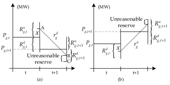
Figure 1.
Unresponsive reserve from a generator due to time coupling. (a) The unresponsive downward reserve capacity. (b) The unresponsive upward reserve capacity.
In Figure 1a, is greater than ; the up-regulated spinning reserve capacity provided by unit g in time period t is . Let it be released as x, the maximum down-regulated power of unit g in a single time period is ; then, in time period t + 1, the operating point of the unit can only go from point A to point B at most, and the part B-C of the down-regulated spinning reserve capacity provided by unit g in time period t + 1 becomes an unresponsive reserve capacity. Similarly, when , the release of may also result in an unresponsive upward reserve capacity in due to the limitation of the maximum upward power of unit g in the time period, as shown in Figure 1b.
In general, if the reserve capacity and active power base-point settings provided by unit g on adjacent time periods satisfy the following conditions:
then, due to the upward release of , there will be an unresponsive downward reserve capacity in . The resulting response risk, i.e., the unresponsive downward reserve capacity expectation, is expressed as:
where is the time-period coupling response risk of down-regulating rotary reserve capacity provided by unit g at time period t + 1; is the action probability density function of the reserve capacity of unit g at time period t, which is determined by the reserve release strategy of the system and the prediction error distribution of random quantities. Its specific expression is given in the next section. The second term in the integral refers to the down-regulated reserve capacity in that cannot respond when is up-regulated and x is released. Let x be positive when the rotary reserve capacity is released up and negative when the rotary reserve capacity is released down.
Similarly, if unit g satisfies the following conditions:
then the release of will generate a response risk in , triggered by the time-period coupling with a risk expression of:
where is the time-period coupling response risk provided by unit g at time period t + 1 to increase the spinning reserve capacity; the second term in the integral is the up-regulated reserve capacity in that cannot respond when releases |x|.
As a result, the response risk of the reserve capacity provided by unit g in time period t + 1 due to coupling ties in adjacent time periods, which can be expressed as:
2.2. Unified Calculation of Spinning Reserve Response Risk
Considering that the time-coupled response risk mainly describes the response risk in AGC capacity release, and to ensure the consistency of AGC capacity and accidental reserve capacity response risk level, this paper organically unifies the reserve response risk caused by forced outage of units into the time-coupled response risk, and gives a unified expression of spinning reserve response risk.
Equation (12) shows the effect of the forced outage of the unit on the participation factors of the available units. The power generation of the forced outage unit needs to be replaced by the release of the spinning reserve capacity of the remaining units, so the action probability density function of the available unit reserve capacity is shifted to the right, as shown in (11). Equations (9) and (10) indicate the impact of the forced outage of the unit on the time-coupling response risk of the available unit reserve. After the unit is forced to the outage, its spinning reserve capacity is completely invalid, as shown in (7) and (8).
3. Uncertainty in Dynamic Economic Dispatch
3.1. Uncertainty Description of Load
System load can be expressed by the sum of short-term forecasting and forecasting errors, namely:
Given the periodicity of the load and the maturity of the load forecasting, the standard deviation of the load forecasting error within the short-term forecasting range can be expressed as a percentage of the predicted load value:
3.2. Uncertainty of Wind Power
If the system contains a large number of fans with rich geographical diversity, it can also be assumed that the actual value of wind power is equal to the predicted value plus the normal distribution error.
The relative error in wind power forecasting is greater than the load. In addition, the standard deviation of this error increases with the forecast time scale. In [24], the standard deviation of the wind power prediction error is plotted as a function of the standardized predicted power for a collection of wind farms included in a 140 km diameter region, and the standard deviation of the wind power prediction error can be expressed as:
3.3. Uncertainty Description of Net Load
System net load demand is the difference value between load and wind power:
where, is the error of the combination of load and wind power forecasting error, which obeys the Gaussian distribution with a mean value of zero. Because the load is not related to the wind power forecasting error, its standard deviation is .
3.4. Uncertainty Description of Spinning Reserve Release
The effect of forced unit shutdown on system reserve release is given in Section 1, and only the release model for the reserve provided by the unit in the non-failure condition is given here.
In the non-fault condition, the main role of the spinning reserve is to smooth the power imbalance caused by the prediction error of load and intermittent power output, so the action distribution in the spinning reserve is directly collinear with the prediction error distribution in the net system load. If the release strategy of unit reserve is assigned by participation factor, the action probability density function of each unit reserve with known net load prediction error distribution can be expressed as:
The derivation process follows: is the probability that the net load forecast error is A. If unit g is not limited by reserve capacity, the reserve it needs to release is , and the action probability is also ; replacing with x, the probability density function of unit g reserve action is when ; similarly, the action probability density function of the remaining parts can be derived.
4. Optimization Model for Dynamic Economic Dispatch
4.1. Objective Function
The dispatch target is the minimum sum of the power generation cost of the system, the user’s expectation of power failure loss, and the expectation of wind abandonment loss:
The first term in (19) is the total fuel cost of a conventional unit, wherein the fuel cost of the unit taking into account the valve point effect [25] is:
The second term in (19) is the customer outage loss expectation, where the power shortage expectation due to insufficient system up-spinning reserve is:
The third term in (19) is the expectation of wind abandonment loss, which results in wind abandonment when the system that takes into account the response risk reduces the spinning reserve capacity to be insufficient, and the expectation of wind abandonment loss power is:
If considered from the perspective of traditional economic dispatch problems, the cost of wind abandonment in the objective function, i.e., AWAR, can be set to 0, because if the solution of optimal dispatch produces wind abandonment, it indicates that the cost of absorbing this part of wind power is higher than the fuel consumption cost of conventional units producing the same amount of electricity. However, if social benefits such as environmental protection are further considered, it is necessary to set a certain cost for wind abandonment. This article sets the value of AWAR from the perspective of carbon trading value as:
4.2. Constraints
The following constraints need to be satisfied in the objective search of (20).
- Active power balance constraints in each period:
- The output power capacity constraints for each unit in each period:
- Constraints on setting reserve capacity for each unit in each period:where the limitation of the first items and of the min function ensures that the unit g can completely release the set reserve capacity during the period; the second limitation is to ensure that when the reserve capacity is fully released in that period, the active power output base point of the unit in the next period can be achieved.
The DED model illustrated in (19)–(28) is one of the implementations of the approach proposed in this paper. The central advancement of the DED model proposed in this paper over existing DED models is that it takes into account the response risk of the spinning reserve provided by the unit due to flexibility constraints. To apply the proposed method to an existing AGC program, such as Siemens’ commercial AGC program, it is only necessary to calculate the spinning reserve response risk according to (6)–(12). Then, the spinning reserve response risk can be removed from the reserve capacity, and the actual effective reserve capacity of the unit is obtained, replacing the original reserve capacity. The specific expression of effective reserve can be adjusted according to the type of DED model (e.g., stochastic model, robust model). The DED model proposed in this paper can be further extended to other forms of renewable energy sources such as photovoltaic, and the key problem to be solved is how to unify the different uncertainty distributions in various types of renewable energy sources and derive the uncertainty description of spinning reserve release, which is the next step of this paper.
5. Solution of Dynamic Economic Dispatch Optimization Model
In this paper, an improved multi-universe parallel quantum genetic algorithm is used to solve the proposed dynamic economic dispatch optimization model. Among them, the adaptive Simpson integral method is used in the numerical calculation of the integration of the objective function. In addition, considering the relatively small probability of multiple faults during the dispatching time, this paper adopts the simplified treatment of indicators such as the probability of loss of load in the calculation of the commissioning risk degree in [26], and the EENS,t and EWEA,t are calculated by solving the two faults.
Similar to the multi-population genetic algorithm [27], the multi-universe parallel quantum genetic algorithm also has the problem that it is difficult to select the information exchange rate between populations. When too much information is exchanged, it reduces the diversity of individuals within various populations, loses the parallel algorithm’s feature of searching in multiple directions simultaneously, and reduces the algorithm’s global superiority-seeking ability. When too little information is exchanged in the populations, it again leads to ineffective propagation of outstanding individuals and reduces the convergence speed of the algorithm [28]. For this reason, this paper improves the multi-universe parallel topology of the multi-universe parallel quantum genetic algorithm by dividing the universes into main universes and minor universes. The small universes can only be attached to a specific main universe, and the information can only be transmitted in the direction from the small universe to the main universe it is attached to, or between different main universes. In this way, on the one hand, the individual diversity and independent evolution characteristics of the small universe are maintained, and at the same time, the independent characteristics of the small universe can also be transmitted to the main universe attached to it, maintaining a certain difference between the main universes, and ensuring the breadth of the algorithm’s search space; on the other hand, by adopting the optimal migration strategy, the excellent individuals in the small universes can also be effectively propagated in the main universes, ensuring the convergence of the algorithm. The improved multi-universe parallel superstar row structure is shown in Figure 2. Since only the parallel topology structure is improved, it is equivalent to a special form of the original multi-universe parallel quantum genetic algorithm, and the global convergence of the algorithm remains unchanged [29].
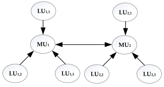
Figure 2.
Improved multi-universe superstar structure. MU denotes the main universe and LU denotes the small universe.
Taking the active base point and spinning reserve capacity setting of each conventional unit in each period as individual genes, the algorithm flow of solving the dynamic economic dispatch model based on the improved multi-universe parallel quantum genetic algorithm is shown in Figure 3. Among them, the multi-universe parallel topology structure is shown in Figure 2. The specific implementation of multi-state genetic quantum bit encoding, quantum rotating gate and non-gate evolution, and optimal migration and quantum crossover operation can be found in [29].
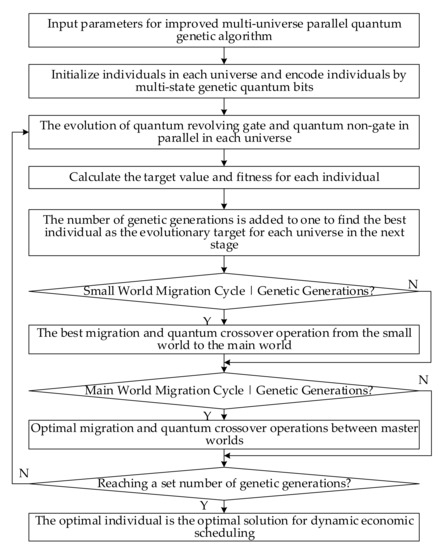
Figure 3.
Flowchart of the improved multi-universe parallel quantum genetic algorithm.
6. Example Analysis
This paper uses Matlab-R2019b to write a test program, and uses the CUDA (Compute Unified Device Architecture) toolbox to call GPU accelerated parallel operations. The CUDA programming model uses CPU as the host and GPU as the co-processor. CPU is responsible for logical transaction processing and serial computing; GPU focuses on performing parallel processing tasks. The improved multi-universe parallel quantum genetic algorithm used in this paper is suitable for the CUDA programming model. GPU (GeForce GTX 1650) is responsible for independent parallel evolution in each universe, and CPU (Intel i5-9300H) is responsible for optimal migration and quantum cross-operation between universes.
The constructed 10-unit system is used as an arithmetic example to verify the method of this paper. The characteristic data of each unit are shown in Table A1 in the Appendix A. The load and wind power forecast data are used from actual forecast data, publicly available for the Irish grid [30], as shown in Figure 4. The length of a single time period for dynamic economic dispatch is 15 min, and the number of forward-looking periods T is 16 (see reference [24] for the selecting the number of forward periods). The current share of wind power generation in the Irish grid is about 50–60% [30], and the total wind power generation in the example of this paper accounts for 43.9% of the total load power. The parameters in the model follow: z takes 2 [31]; and take 0.15 and 0.018 [31], respectively; IEAR takes 4 USD/S [16]; PCO2 takes 10 USD/t [32].
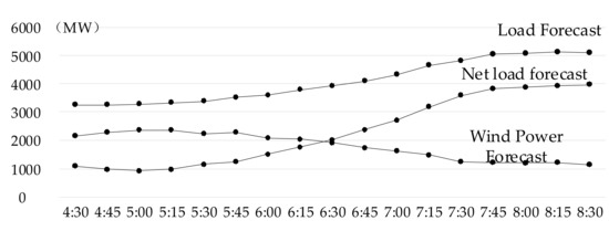
Figure 4.
Forecast data of load and wind power.
The parameters of the improved multi-universe parallel quantum genetic algorithm are as follows: the number of genetic generations is 100; the number of main universes is 4; the number of small universes attached to each main universe is 3; the number of individuals in each main universe is 40; the number of individuals in each small universe is 30; the migration scale between main universes is 10%, the migration period is 8 generations, and the selection probability of quantum crossover is 20%; the migration scale of small universes to main universes is 10%, the migration period is 4 generations, and the selection probability of quantum crossover is 30%; the probability of quantum mutation in each small universe is 20%; the probability of quantum mutation in each main universe is 10%.
6.1. Impact Analysis of Unit Regulation Rate Constraint Forms
Initially, in order to analyze the impact of different forms of unit regulation rate constraints on dynamic economic dispatch, the following three models are used to optimize the dispatch of the test system: this research model (referred to as M1); on the basis of this research model, the greater-than signs in (1) and (3) are changed to less-than or equal-to signs, and they are added to the constraints, so that it is ensured that the unit reserve will not generate response risk due to time coupling, i.e., using the unit regulation rate constraint form given in [33] (referred to as M2); on the basis of this research model, the time-coupled response risk of the reserve is no longer calculated, and (28) and (29) are changed to the traditional unit reserve capacity constraint and unit regulation rate constraint form (referred to as M3).
The specific situation for each model dispatch solution is shown in Table 1. Table 1 also presents the spinning reserve capacity set for unit 6 during the period 7:00–7:15 to facilitate illustration of the impact of different forms of regulation rate constraints on the reserve capacity setting for each model unit.

Table 1.
Comparison of optimal dispatch solutions for each model.
Unit 6 is in the mid-range operation during the period 7:00–7:15, and for M3 using the conventional unit regulation rate constraint, the reserve capacity setting of unit 6 is only limited by its regulation rate, and its set upward and downward spinning reserve capacities are both 36 MW, but as can be seen in Figure 4, the net system load is in the rising phase during the period 7:00–7:15, and the unit 6 base point needs to be adjusted for climbing, so that the release of unit 6’s downward spinning reserve capacity will lead to more time-coupled response risk in its upward spinning reserve in the next period, as shown in Figure 1; its expectation of user outage loss in the next period will be increased in order to reduce the expectation of wind abandonment loss during this period. M3 has set the highest reserve capacity, but it does not consider the response risk from time coupling, resulting in the highest expectation of customer outage loss and the highest total reserve response risk.
In contrast, in order to ensure that no time-coupled response risk is generated at all, M2 allows the unit to set a very small downward spinning reserve capacity during the unit climbing phase, which leads to an increase in the expectation of wind abandonment losses, while the spinning reserve capacity set for the unit in M2 is also more restricted during the net load drop and relatively flat phase; i.e., it leads to a larger restriction on the reserve capacity release in this time period in order not to generate time-coupled response risk in the next time period. Although M2 recognizes the time-coupled response risk of reserve, it still wants to continue the traditional idea of deterministic reserve: unit failure is a small probability event and unit reserve capacity can be considered to be available with a high probability of certainty. The total reserve response risk of M2, triggered only by unit failure, is minimal, but its total cost is instead the highest.
From this example, it can be seen that the method in this paper allows a certain uncertainty in reserve setting (time-period coupling response risk), and no longer requires reserve to be deterministic according to the traditional thinking, but takes the total social benefit as the index, and the reserve setting takes into account the reserve response risk caused by the forced outage of the unit and time coupling, which ensures the consistency of the system response risk in each time period and reduces the operation whose total cost is minimal.
6.2. Analysis of the Impact of Wind Power Volatility and Uncertainty
In order to analyze the impact of wind power volatility and uncertainty on dynamic economic dispatch, the following scenarios are constructed based on the original test scenario (S1): no wind power volatility scenario (S2) [34], where wind power output is constant and its value is the average value of the original wind power output during the dispatch time; no wind power uncertainty scenario (S3), where wind power prediction error is 0; no wind power volatility and uncertainty scenario (S4), the wind power output is a constant mean value, and the wind power prediction error is 0.
Dynamic economic scheduling is performed for each scenario using the methods described in this paper. Table 2 shows the total cost of the dispatch solution and the total reserve response risk for each scenario. The total cost of the dispatch solution and the total reserve response risk for each scenario decrease from S1 to S4. S4 is a scenario without wind power fluctuation and uncertainty, so its dispatch solution cost can be used as a benchmark value; the cost of S3 is subtracted from it to obtain the cost of wind power volatility of 0.0899 MUSD; the cost of S2 is subtracted from it to obtain the cost of wind power uncertainty of 0.3446 MUSD; and the cost of S1 is subtracted from it to obtain the cost of wind power volatility and uncertainty together at 0.6217 MUSD.
Table 2.
Impact of wind power volatility and uncertainty.
This example shows that the cost of wind power uncertainty in this example case is higher than the cost of wind power volatility, but the increase in dispatch cost due to wind power volatility and uncertainty together is higher than the sum of the increase in cost due to volatility and uncertainty alone. Similarly, the increase in standby response risk due to wind volatility and uncertainty together is higher than the sum of volatility and uncertainty alone.
6.3. Algorithm Performance Analysis
In order to verify the performance of the improved multi-universe parallel quantum genetic algorithm, a reference comparison with the traditional genetic algorithm [35] and the multi-universe parallel quantum genetic algorithm [36] was performed; the results are shown in Figure 5. The improved multi-universe parallel quantum genetic algorithm converges to stability and reaches the optimal solution in forty generations, while the multi-universe parallel quantum genetic algorithm converges to stability and reaches the optimal solution only when it approaches 80 generations, and the convergence speed and search performance of the traditional genetic algorithm are inferior to the other two.
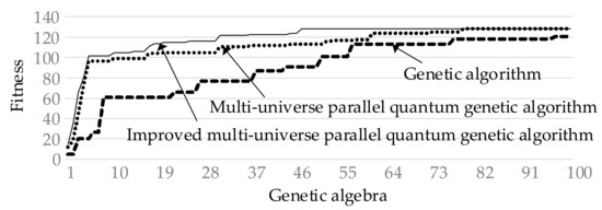
Figure 5.
Algorithm performance comparison.
In terms of algorithm speed, the average algorithm time in the calculation of the arithmetic cases is about 130 s with the CUDA programming model, while the conventional genetic algorithm without GPU parallel acceleration (with a population size of 100) takes about 14 min.
7. Conclusions
This study presents a calculation method to analyze the response risk due to the coupling drawback between time periods for the spinning reserve provided by conventional units in the dispatch, the reserve response risk caused by forced outages of units is considered, and, finally, a unified expression of spinning reserve response risk is given. A new dynamic economic dispatch model for integrating high levels of wind power into a power system is proposed, which can ensure the consistency of the system response risk in each time period by considering the expectation of customer outage loss and the expectation of wind abandonment loss in the objective function. By improving the parallel universe topology, the convergence and computational speed of the multi-universe parallel quantum genetic algorithm are improved. The results analyzed from an example prove the effectiveness of the model described in this paper, and conclusions are as follows:
- For coping with the fluctuation and uncertainty of wind power, adjustable resources are needed in dispatch; therefore, the containment of the reserve provided by adjustable resources is enhanced significantly in time intervals. The utilization of traditional deterministic methods could increase dispatch cost significantly by forcing the reserve available at 100%, and it may increase the risk of wind power curtailment and load abandonment in the dispatch during conditions of limited adjustable resources. Therefore, it is necessary to allow and consider carefully the uncertainty of reserve in dispatching (response risk), and pursue a balance between economy and reliability.
- The joint effects of fluctuation and uncertainty of wind power on the response risk of spinning reserve in dispatch are greater than the sum of their separate effects; therefore, the fluctuation and uncertainty of wind power need to be considered organically and uniformly in dispatch. If the fluctuation and uncertainty of wind power were considered separately, decisions in dispatch may be more radical.
- By improving the topology structure of the parallel universe, in which the main universe and the little universe are divided, and specifying the direction of information flow, the performance of the multi-universe parallel quantum genetic algorithm can be improved more significantly.
Author Contributions
Y.P. proposed the research topic, designed the model, performed the simulations, and analyzed the data. X.H. was responsible for guidance, proposing the research topic, giving constructive suggestions, and revising the paper. P.Y. performed the simulations and analyzed the data. Y.Z. improved the manuscript and corrected spelling and grammar mistakes. L.Z. analyzed the data. All authors have read and agreed to the published version of the manuscript.
Funding
This work is supported by the National Natural Science Foundation of China (52107111) and Shandong Provincial Natural Science Foundation (ZR2022ME219, ZR2021QE117). The authors also acknowledge support from the Key Laboratory of Power System Intelligent Dispatch and Control, Ministry of Education, Shandong University.
Data Availability Statement
Not applicable.
Acknowledgments
This work is supported by the National Natural Science Foundation of China (52107111) and Shandong Provincial Natural Science Foundation (ZR2022ME219, ZR2021QE117).
Conflicts of Interest
The authors declare no conflict of interest.
Nomenclature
| Pg,t | The active power output of unit g at time period t | System wind power forecast in time t | |
| t | Index of time | Wind power forecast error | |
| g | Index of unit | Standard deviation of wind power forecast errors | |
| Up-regulated spinning reserve capacity provided by unit g at time t | Total installed capacity of wind power | ||
| x | Reserve capacity released | Corresponding coefficients when the predicted duration is T | |
| Maximum downward power of the unit g in a period time | Corresponding coefficients when the predicted duration is T | ||
| Downshifting reserve capacity provided by unit g at time t + 1 | T | Prospective period of dynamic economic dispatch single period | |
| Maximum up-regulated power of unit g during a time period | The difference between load and wind power | ||
| Down-regulated spinning reserve capacity provided by unit g at time t | Errors in the combination of load and wind power forecast errors | ||
| Upshifting reserve capacity provided by unit g at time t + 1 | Action probability density function for each unit reserve | ||
| Time coupled response risk for the downward spinning reserve capacity provided by unit g at time t + 1 | Probability of net load forecast error of A abandonment of the system in time t | ||
| ρg,t | Action probability density function of unit g reserve capacity at time t | N | Number of system units |
| Time coupling response risk for the upward spinning reserve capacity provided by unit g at time t + 1 | Cg | Generation fuel cost of the unit g | |
| Total system spinning reserve response risk in time period t | IEAR | Blackout loss evaluation rate | |
| Upward spinning reserve response risk in time period t | Low power expectation due to insufficient system up-regulation spinning reserve | ||
| Downward spinning reserve response risk in time period t | AWAR | Evaluation of wind abandonment losses | |
| The probability that the system is in state k during the t-period | Expectation of electricity loss from wind abandonment | ||
| U | The set of unavailable units under state k | Unit fuel costs taking into account valve point Effects | |
| A | The set of available units under state k | Fuel cost factor | |
| Time-coupled response risk for upward spinning reserve of available units g in state k at time slot t | Fuel cost factor | ||
| Time-coupled response risk for downward spinning reserve of available units g in state k at time slot t | Fuel cost factor | ||
| Action probability density function of available unit g reserve under t period state k | Fuel cost factor | ||
| Participation factor for reserve release of unit g in the normal state in time period t | Fuel cost factor | ||
| Participation factor for reserve release of unit g in the state k in time period t | Minimum technical output power of the unit g | ||
| System load forecast value in time t | Carbon emission intensity per unit of electricity of unit g | ||
| Load forecast error | Carbon trading price | ||
| Standard deviation of load forecast error | Upper limit of unit g output power | ||
| Wind power actual value | Lower limit of unit g output power |
Appendix A
Table A1.
Conventional generator parameters.
Table A1.
Conventional generator parameters.
| Unit | Active Upper Limit (MW) | Active Lower Limit (MW) | ag USD/(MW)2·h | bg USD/(MW)·h | cg 10−3USD/h | dg USD/h | eg Rad/MW | MW/min | kg/MW·h | Failure Rate (×10−5) |
|---|---|---|---|---|---|---|---|---|---|---|
| 1 | 200 | 40 | 38.3543 | 1.3768 | 3.1508 | 21.66 | 0.038 | 1 | 945 | 4 |
| 2 | 300 | 60 | 49.6535 | 1.2643 | 2.8904 | 27.93 | 0.042 | 1.5 | 911 | 2 |
| 3 | 650 | 120 | 100.7425 | 0.8585 | 1.8545 | 57 | 0.036 | 3.25 | 790 | 1 |
| 4 | 620 | 110 | 121.5446 | 0.7423 | 1.6704 | 68.97 | 0.052 | 3.1 | 810 | 1 |
| 5 | 680 | 135 | 105.7976 | 0.7643 | 1.7448 | 59.85 | 0.068 | 3.4 | 782 | 1 |
| 6 | 480 | 90 | 89.4235 | 0.9954 | 2.1780 | 50.73 | 0.049 | 2.4 | 843 | 2 |
| 7 | 650 | 115 | 102.4523 | 0.7782 | 1.7884 | 58.14 | 0.034 | 3.25 | 762 | 2 |
| 8 | 520 | 95 | 87.7874 | 0.9428 | 1.9690 | 49.59 | 0.035 | 2.6 | 849 | 3 |
| 9 | 320 | 65 | 91.7594 | 1.0213 | 1.9849 | 51.87 | 0.048 | 1.6 | 879 | 2 |
| 10 | 350 | 50 | 133.6109 | 0.7244 | 1.4741 | 75.81 | 0.026 | 1.75 | 860 | 5 |
References
- Peng, F.; Gao, Z.; Hu, S.; Zhao, W.; Sun, H.; Wang, Z. Bilateral Coordinated Dispatch of Multiple Stakeholders in Deep Peak Regulation. IEEE Access 2020, 8, 33151–33162. [Google Scholar] [CrossRef]
- Mai, T.; Hand, M.M.; Baldwin, S.F.; Wiser, R.H.; Brinkman, G.L.; Denholm, P.; Arent, D.J.; Porro, G.; Sandor, D.; Hostick, D.J. Renewable Electricity Futures Study; Colorado: National Renewable Energy Laboratory: Golden, CO, USA, 2014. [Google Scholar]
- Schellekens, G.; Battaglini, A.; Lilliestam, J.; McDonnell, J.; Patt, A. 100% Renewable Electricity: A Roadmap to 2050 for Europe and North Africa 2013; Pricewaterhouse Coopers: London, UK, 2010; pp. 1–13. [Google Scholar]
- Wang, M.; Yang, M.; Fang, Z.; Wang, M.; Wu, Q. A Practical Feeder Planning Model for Urban Distribution System. IEEE Trans. Power Syst. 2020. [Google Scholar] [CrossRef]
- Li, P.; Yang, M.; Yu, Y.; Hao, G.; Li, M. Decentralized Distributionally Robust Coordinated Dispatch of Multiarea Power Systems Considering Voltage Security. IEEE Trans. Ind. Appl. 2021, 57, 3441–3450. [Google Scholar] [CrossRef]
- Javadi, M.S.; Lotfi, M.; Gough, M.; Nezhad, A.E.; Santos, S.F.; Catalão, J.P.S. Optimal Spinning Reserve Allocation in Presence of Electrical Storage and Renewable Energy Sources. In Proceedings of the 2019 IEEE International Conference on Environment and Electrical Engineering and 2019 IEEE Industrial and Commercial Power Systems Europe (EEEIC/I&CPS Europe), Genova, Italy, 11–14 June 2019; pp. 1–6. [Google Scholar]
- Guo, Z.; Wu, W. Data-Driven Model Predictive Control Method for Wind Farms to Provide Frequency Support. IEEE Trans. Energy Convers. 2022, 37, 1304–1313. [Google Scholar] [CrossRef]
- Ye, L.; Zhang, C.; Tang, Y.; Zhong, W.; Zhao, Y.; Lu, P.; Zhai, B.; Lan, H.; Li, Z. Hierarchical Model Predictive Control Strategy Based on Dynamic Active Power Dispatch for Wind Power Cluster Integration. IEEE Trans. Power Syst. 2019, 34, 4617–4629. [Google Scholar] [CrossRef]
- Han, X.S.; Gooi, H.B.; Kirschen, D.S. Dynamic Economic Dispatch: Feasible and Optimal Solutions. IEEE Trans. Power Syst. 2001, 16, 22–28. [Google Scholar] [CrossRef]
- Chen, Z.; Zhu, G.; Zhang, Y.; Ji, T.; Liu, Z.; Lin, X.; Cai, Z. Stochastic Dynamic Economic Dispatch of Wind-Integrated Electricity and Natural Gas Systems Considering Security Risk Constraints. CSEE J. Power Energy Syst. 2019, 5, 324–334. [Google Scholar]
- Alanazi, M.S. A Modified Teaching—Learning-Based Optimization for Dynamic Economic Load Dispatch Considering Both Wind Power and Load Demand Uncertainties with Operational Constraints. IEEE Access 2021, 9, 101665–101680. [Google Scholar] [CrossRef]
- Lee, T.Y. Optimal Spinning Reserve for A Wind-Thermal Power System Using EIPSO. IEEE Trans. Power Syst. 2007, 22, 1612–1621. [Google Scholar] [CrossRef]
- Wu, L.; Li, Z.; Xu, Y.; Zheng, X. Stochastic-Weighted Robust Optimization Based Bi-layer Operation of A Multi-energy Home Considering Practical Thermal Loads and Battery Degradation. IEEE Trans. Sustain. Energy 2021, 13, 668–682. [Google Scholar]
- Wang, M.; Wu, Y.; Yang, M.; Wang, M.; Jing, L. Dynamic Economic Dispatch Considering Transmission–Distribution Coordination and Automatic Regulation Effect. IEEE Trans. Ind. Appl. 2022, 58, 3164–3174. [Google Scholar] [CrossRef]
- Zaman, M.F.; Elsayed, S.M.; Ray, T.; Sarker, R.A. Evolutionary Algorithms for Dynamic Economic Dispatch Problems. IEEE Trans. Power Syst. 2016, 31, 1486–1495. [Google Scholar] [CrossRef]
- Gu, C.; Wu, J.; Li, F. Reliability-Based Distribution Network Pricing. IEEE Trans. Power Syst. 2012, 27, 1646–1655. [Google Scholar] [CrossRef]
- Li, Z.; Wu, L.; Xu, Y. Risk-Averse Coordinated Operation of a Multi-energy Microgrid Considering Voltage/Var Control and Thermal Flow: An Adaptive Stochastic Approach. IEEE Trans. Smart Grid 2021, 12, 3914–3927. [Google Scholar] [CrossRef]
- Patel, R.; Li, C.; Meegahapola, L.; McGrath, B.; Yu, X. Enhancing Optimal Automatic Generation Control in a Multi-Area Power System with Diverse Energy Resources. IEEE Trans. Power Syst. 2019, 34, 3465–3475. [Google Scholar] [CrossRef]
- Navid, N.; Rosenwald, G. Market Solutions for Managing Ramp Flexibility with High Penetration of Renewable Resource. IEEE Trans. Sustain. Energy 2012, 3, 784–790. [Google Scholar] [CrossRef]
- Lu, Z.; Li, H.; Qiao, Y. Probabilistic Flexibility Evaluation for Power System Planning Considering Its Association with Renewable Power Curtailment. IEEE Trans. Power Syst. 2018, 33, 3285–3295. [Google Scholar] [CrossRef]
- Zafeiropoulou, M.; Mentis, I.; Sijakovic, N.; Terzic, A.; Fotis, G.; Maris, T.I.; Vita, V.; Zoulias, E.; Ristic, V.; Ekonomou, L. Forecasting Transmission and Distribution System Flexibility Needs for Severe Weather Condition Resilience and Outage Management. Appl. Sci. 2022, 12, 7334. [Google Scholar] [CrossRef]
- Sijakovic, N.; Terzic, A.; Fotis, G.; Mentis, I.; Zafeiropoulou, M.; Maris, T.I.; Zoulias, E.; Elias, C.; Ristic, V.; Vita, V. Active System Management Approach for Flexibility Services to the Greek Transmission and Distribution System. Energies 2022, 15, 6134. [Google Scholar] [CrossRef]
- Wu, C.; Hug, G.; Kar, S. Risk-Limiting Economic Dispatch for Electricity Markets with Flexible Ramping Products. IEEE Trans. Power Syst. 2016, 31, 1990–2003. [Google Scholar] [CrossRef]
- Billinton, R.; Allan, R.N. Reliability Evaluation of Power Systems; Springer Science & Business Media: Berlin, Germany, 1996; pp. 215–224. [Google Scholar]
- Ortega-Vazquez, M.A.; Kirschen, D.S. Estimating the Spinning Reserve Requirements in Systems with Significant Wind Power Generation Penetration. IEEE Trans. Power Syst. 2009, 24, 114–124. [Google Scholar] [CrossRef]
- Fabbri, A.T.; Roman, G.S.; Abbad, J.R.; Quezada, V.H.M. Assessment of The Cost Associated with Wind Generation Prediction Errors in A Liberalized Electricity Market. IEEE Trans. Power Syst. 2005, 20, 1440–1446. [Google Scholar] [CrossRef]
- Yu, Y.; Han, X.; Yang, M.; Yang, J. Probabilistic Prediction of Regional Wind Power Based on Spatiotemporal Quantile Regression. IEEE Trans. Ind. Appl. 2020, 56, 6117–6127. [Google Scholar] [CrossRef]
- Li, Z.; Xu, Y.; Feng, X.; Wu, Q. Optimal Deployment of Heterogeneous Energy Storage System in a Residential Multi-Energy Microgrid with Demand Side Management. IEEE Trans. Ind. Inform. 2020, 17, 991–1004. [Google Scholar] [CrossRef]
- Doherty, R.; O’Malley, M. A New Approach to Quantify Reserve Demand in Systems with Significant Installed Wind Capacity. IEEE Trans. Power Syst. 2005, 20, 587–595. [Google Scholar] [CrossRef]
- Wind and Load Dataset Available from Eirgrid Website. Available online: http://www.Eirgrid.com (accessed on 3 March 2020).
- Li, Z.; Xu, Y. Multiobjective Coordinated Energy Dispatch and Voyage Scheduling for a Multienergy Ship Microgrid. IEEE Trans. Ind. Appl. 2019, 1, 1–9. [Google Scholar]
- Carbon Trading Website. Available online: http://www.tanpaifang.com/ (accessed on 12 May 2021).
- Bouffard, F.; Galiana, F.D. An Electricity Market with A Probabilistic Spinning Reserve Criterion. IEEE Trans. Power Syst. 2004, 19, 300–307. [Google Scholar] [CrossRef]
- Han, K.; Kim, J.H. Genetic Quantum Algorithm and its Application to Combinatorial Optimization Problem. In Proceedings of the Proceedings of the 2000 Congress on Evolutionary Computation. CEC00 (Cat. No.00TH8512), La Jolla, CA, USA, 16–19 July 2000. [Google Scholar]
- Yang, J.N.; Li, B.; Zhuang, Z.Q. Multi-Universe Parallel Quantum Genetic Algorithm Its Application to Blind-Source Separation. In Proceedings of the International Conference on Neural Networks and Signal Processing, Nanjing, China, 14–17 December 2003; Volume 1, pp. 393–398. [Google Scholar]
- Zhang, J.; Lu, C.; Song, J.; Zhang, J. Real-time AGC Dispatch Units Considering Wind Power and Ramping Capacity of Thermal Units. J. Mod. Power Syst. Clean Energy 2015, 3, 353–360. [Google Scholar] [CrossRef]
Publisher’s Note: MDPI stays neutral with regard to jurisdictional claims in published maps and institutional affiliations. |
© 2022 by the authors. Licensee MDPI, Basel, Switzerland. This article is an open access article distributed under the terms and conditions of the Creative Commons Attribution (CC BY) license (https://creativecommons.org/licenses/by/4.0/).