Article

SSA-LSTM: Short-Term Photovoltaic Power Prediction Based on Feature Matching

1
College of Economics & Management, China Three Gorges University, Yichang 443000, China
2
College of Electrical Engineering & New Energy, China Three Gorges University, Yichang 443000, China
3
College of Computer and Information Technology, China Three Gorges University, Yichang 443000, China
*
Author to whom correspondence should be addressed.
Energies 2022, 15(20), 7806; https://doi.org/10.3390/en15207806
Submission received: 16 September 2022 / Revised: 13 October 2022 / Accepted: 15 October 2022 / Published: 21 October 2022
(This article belongs to the Section A2: Solar Energy and Photovoltaic Systems)

Abstract

:
To reduce the impact of volatility on photovoltaic (PV) power generation forecasting and achieve improved forecasting accuracy, this article provides an in-depth analysis of the characteristics of PV power outputs under typical weather conditions. The trend of PV power generation and the similarity between simultaneous outputs are found, and a hybrid prediction model based on feature matching, singular spectrum analysis (SSA) and a long short-term memory (LSTM) network is proposed. In this paper, correlation analysis is used to verify the trend of PV power generation; the similarity between forecasting days and historical meteorological data is calculated through grey relation analysis; and similar generated PV power levels are searched for phase feature matching. The input time series is decomposed by singular spectrum analysis; the trend component, oscillation component and noise component are extracted; and principal component analysis and reconstruction are carried out on each component. Then, an LSTM network prediction model is established for the reconstructed subsequences, and the external feature input is controlled to compare the obtained prediction results. Finally, the model performance is evaluated through the data of a PV power plant in a certain area. The experimental results prove that the SSA-LSTM model has the best prediction performance.

1. Introduction

In recent years, to address problems such as energy shortages and environmental pollution, the development of renewable energy has become the main direction of the global energy revolution and a key response to climate change [1]. Solar energy has developed rapidly as an efficient, renewable and clean energy source. The global installed photovoltaic (PV) capacity has grown swiftly. According to the global PV report released by the International Energy Agency, by the end of 2021, the cumulative installed capacity reached 942 GW, which is an increase of 22.8% over that in 2020; as such, PV energy has great developmental potential [2]. However, with the continuous increase in the proportion of PV energy, the randomness and volatility of PV outputs have become increasingly prominent, which brings certain difficulties to the operation of a power grid. Therefore, the accurate prediction of PV power generation can help the grid dispatching department to better avoid risks, improve the safety and economy of the power system and be of great significance to the stable operation of the power grid.
In numerous previous studies, scholars carried out research on photovoltaic power generation forecasting, which is mainly divided into two categories: physical models and statistical models. In physical models, the forecast value of solar irradiance and geographic location information, combined with the operation mode of photovoltaic modules, are used to carry out mathematical modeling [3], and the energy storage system is used to solve the negative effects of unstable power generation and low power supply reliability. In practical applications, errors due to power loss and other issues will inevitably occur when using photovoltaic power. Improving material properties is the most direct way to improve photoelectric conversion efficiency [4,5]. At present, scholars have studied the structural characteristics of composite materials to improve the status of photovoltaic applications [6,7]. The rapid development of the photovoltaic industry has brought broad application prospects to the research field of photovoltaic composite materials. In the statistical model, the historical data of photovoltaic power plants is mainly relied upon. Therefore, artificial intelligence algorithms have been favored by scholars. These include machine learning algorithms such as artificial neural networks [8,9] (ANNs) and support vector machines [10,11] (SVMs). These algorithms have been widely used in the field of PV power generation forecasting. For example, the article in [12] proposed an efficient ANN prediction model to study the relationship between meteorological data and PV power generation. The authors of [13] proposed an extended model based on an SVM to obtain a more accurate dataset. The prediction accuracy of machine learning models often depends on the quality of the given dataset and the settings of the internal hyperparameters. Likewise, small dataset differences can lead to significant changes in prediction results [14]. Therefore, hybrid forecasting models have appeared one after another. By optimizing the utilized dataset and calculating the best hyperparameters, a forecasting model can obtain its best forecasting effect. Experiments have shown that the use of the SVM algorithm, after performing particle swarm optimization (PSO) for the parameters, can obtain more accurate prediction results [15]. Usman et al. [16] developed an evaluation framework for short-term PV power prediction and conducted a comparative analysis among various machine learning models and feature selection methods, and the results showed that the extreme gradient boosting (XGBoost) method outperformed individual machine learning methods. According to the authors of [17], by combining XGBoost with feature engineering technology, important information was extracted from weather forecasts to achieve improved prediction accuracy.
Compared with traditional machine learning techniques, deep learning models have better fitting performance and are able to discover intrinsic connections in high-dimensional data [18]. Therefore, a PV prediction model based on deep learning can better mine the intrinsic value of feature data. Deep learning models include convolutional neural networks (CNNs) [19], deep belief networks (DBNs) [20], recurrent neural networks (RNNs), generative adversarial networks (GANs) [21] and other classic models, as well as their variants and combined models. As a variant of an RNN model, a long short-term memory (LSTM) network can effectively capture the long-term dependencies of time series and has become very popular in the field of short-term PV output power prediction. For example, the experimental results in [22] showed that the performance of an LSTM-based PV power generation prediction method is better than that of multilayer perceptrons (MLPs) and deep convolutional networks. The authors of [23] used an LSTM network to predict the solar irradiance on the previous day, and its result was better than those of the backpropagation (BP) neural network and linear least-squares regression. The authors in [24] proposed a CNN-LSTM hybrid deep learning model, which uses a multilayer CNN for feature extraction and an LSTM layer for prediction, thereby effectively improving the prediction effect of the LSTM.
Regardless of the chosen prediction algorithm, the data processing step is a challenge that cannot be ignored. A PV output power sequence has nonlinear characteristics. Decomposing such a time series into multiple subsequences can effectively reduce the complexity of the data and is an effective means for improving the prediction accuracy of the utilized model [25]. Common sequence decomposition methods include empirical mode decomposition (EMD), ensemble EMD (EEMD) and wavelet decomposition (WD) [26,27]. However, the results of the above sequence decomposition methods cause modal aliasing, which increases the difficulty of prediction. As a method that performs sequence decomposition and reconstruction [28], singular spectrum analysis (SSA) can effectively decompose a sequence into a trend sequence, a periodic sequence and a noise sequence without selecting an a priori basis function or a complex operation process, and this technique achieves better objectivity and adaptability [29]. It is suitable for various engineering disciplines and has been widely used in wind power forecasting and power load forecasting [30,31]. For example, [32] decomposed a wind power series into two subsequences (a trend series and a noise series) through SSA and used the hybrid Laguerre neural network to predict the decomposed signals. In [33], a multistep advance wind speed prediction model was proposed by combining variational mode decomposition (VMD) and SSA with an LSTM model.
The processing of weather characteristic data is also an important link in PV power forecasting. Although the PV output power fluctuates, the fluctuation range of the PV output power is similar under the same weather type. Therefore, when constructing a dataset for PV forecasting, clustering the data on similar days according to the associated weather types can reduce data redundancy and forecasting errors [34]. Commonly used clustering methods include K-nearest neighbors (KNN) [35] and K-means clustering (K-means) [36]. The authors of [37] used the fuzzy C-means (FCM) clustering algorithm to cluster and analyze historical meteorological data and weather forecast information, and used the whale optimization algorithm and a least-squares SVM (LSSVM) to make predictions. In [38], K-means clustering was used to select similar historical data from forecasting days as training samples, and then, complete EEMD with adaptive noise (CEEMDAN) and a gated recurrent unit (GRU) were used to forecast PV power. The simulation results showed that the proposed model outperformed other models. It can be seen that when processing PV power generation datasets, whether clustering weather types or searching for similar days, establishing corresponding models for different types of data can improve the resulting prediction accuracy. The above methods slice an entire dataset into many smaller datasets for training a prediction model. When the amount of data is insufficient, the decomposed dataset may be very small, which can easily lead to an insufficient number of training samples for the algorithm and overfitting of the prediction results [39].
In summary, this paper proposes a hybrid forecasting model based on SSA-LSTM. SSA decomposition is performed on the given PV output power sequence with strong volatility; the trend sequence, periodic sequence and noise sequence of the PV output power sequence are extracted; and principal component analysis is performed on the sequence. The important components are extracted for sequence reconstruction, and LSTM prediction models are separately established for the reconstructed sequences. The purpose of this is to enable the LSTM to directly learn regular sequence data, reduce the complexity of the model and improve the prediction accuracy. Existing research lacks in-depth studies on feature information and the law of PV output power. This paper fully mines the characteristics of PV meteorological data, extracts high-quality features and improves the data quality.
To verify the validity of the model, this paper utilizes data from the Ningxia Wuzhong Sun Mountain PV power station [40]. At the same time, we conduct comparative experiments under two frameworks. Model 1 is a time series prediction model, and model 2 incorporates weather features and the feature data constructed in this paper into LSTM prediction. The purpose of this test is to gain insight into the impact of feature data on prediction performance and to verify the effectiveness of the developed method.
The contributions of this paper can be summarized as follows:
  • To improve the quality of the utilized dataset, the PV output power obtained under different weather conditions is analyzed, the law of PV output power is summarized, and a new feature is constructed by combining the PV output law and weather data. The aim is to achieve improved prediction accuracy by mining higher-quality feature data;
  • A short-term PV prediction model (SSA-LSTM) is proposed, in which SSA decomposes nonlinear PV sequences into more regular trend sequences, periodic sequences and noise sequences, reducing the learning complexity of LSTM; the model is combined with feature data to achieve improved prediction accuracy.
The rest of the paper is organized as follows: Second 2 analyzes the characteristics of PV output power and performs feature extraction; Section 3 introduces the forecasting methods and technical descriptions used in this paper; Section 4 presents a case study that validates the validity of the prediction model proposed in this paper using data from the Sun Mountain PV power plant in Wuzhong, Ningxia, China; and Section 5 draws conclusions.

2. PV Power Generation Feature Extraction

There are many factors that affect PV output power. Among them, weather factors have direct impacts on PV output power. This chapter divides weather conditions into four types (sunny, partly cloudy, cloudy and rainy); analyzes the PV output power law in detail under different weather types; and extracts eigenvalues according to the PV output power law.

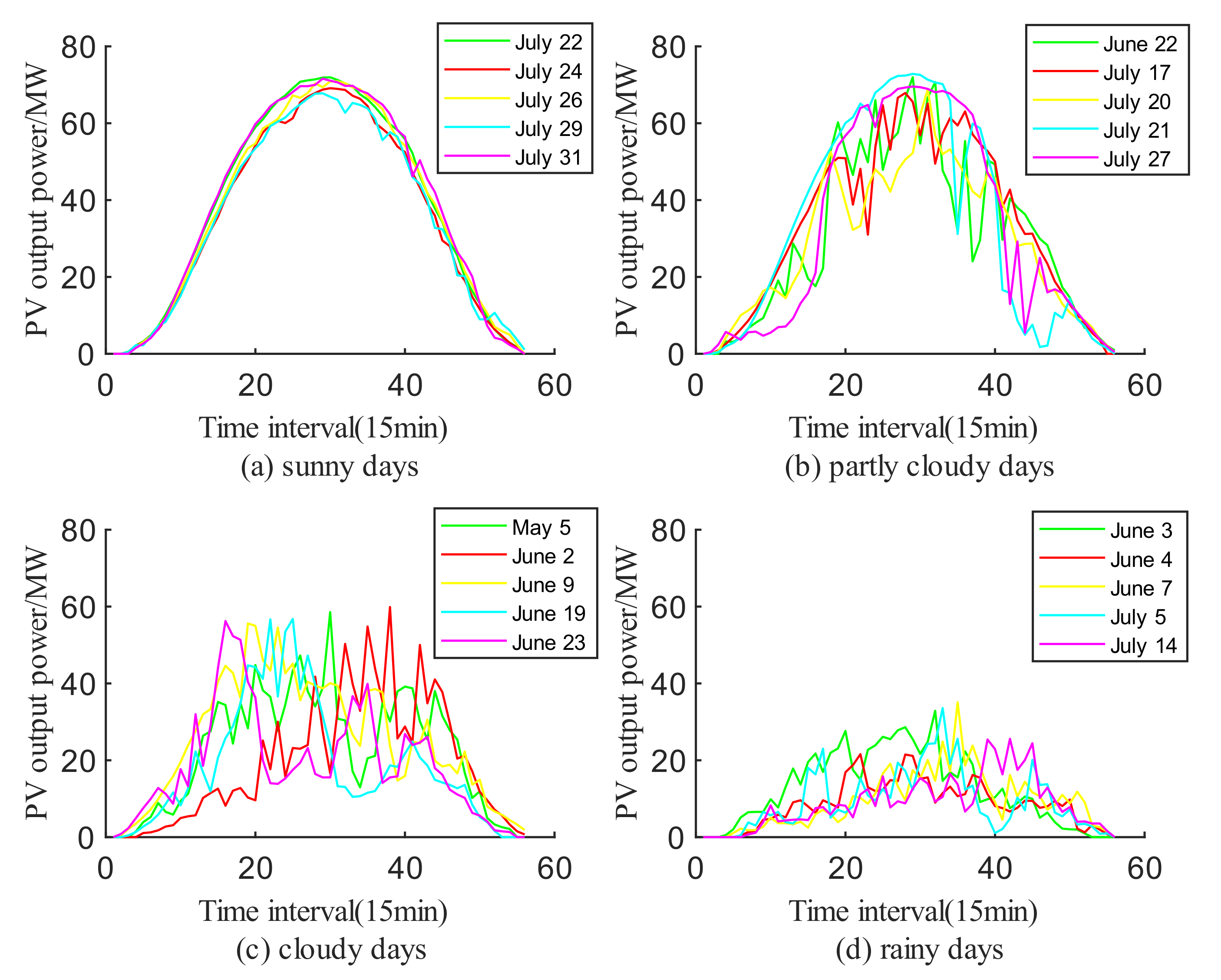
2.1. Typical Form of PV Power Generation

Figure 1 depicts the PV output power produced for five days under four typical weather types: sunny, partly cloudy, cloudy and rainy. The daily comparison is conducted from 5:00 to 18:45, and the sampling interval is 15 min, with a total of 56 nodes per day. Among them, the PV output power levels on sunny days exhibit the highest similarity and are close to the same value. Due to changes in climatic conditions, the fluctuation of PV output power on cloudy, and cloudy and rainy days increases and becomes extremely irregular, and the maximum daily PV output power gradually decreases. When dealing with such problems, some scholars use algorithms to find historically similar days as a training set. The dataset is clustered and analyzed according to its meteorological features, the weather types are divided based on this, and the forecast days are predicted using the data obtained under the same weather type. However, it can be seen from the figure that even under the same weather type, the PV output law exhibits obvious differences. Therefore, it is difficult to capture the power fluctuation characteristics for a whole day based only on the daily matching of similar weather characteristics. At the same time, in a case with a small amount of data, the division of the dataset will reduce the amount of training data, which will reduce the model prediction accuracy to a certain extent. Based on the above two points, it is necessary to conduct a more detailed analysis of the characteristics of PV output power, and conduct feature screening and matching at a finer time granularity to achieve improved prediction accuracy.
As seen from the above figure, the output PV power has a strong trend on sunny days and gradually decreases after gradually increasing to the peak output, showing a hemispherical shape. Although there are no such obvious features for other weather types, from a short-term point of view, the PV output power also forms a short-term increasing or decreasing trend after fluctuation. Therefore, this feature is called the short-term trend of PV output power in this paper. Although it is difficult to find days with similar PV output power, under the same type of weather, the PV output power fluctuates within roughly the same interval. Therefore, it is easier to find similar output points at the same time in history, and at the same time, the quality of the dataset can be improved (that is, made more accurate). Based on the above analysis, feature data for the short-term trend of PV output power and the similarities to power are simultaneously constructed.

2.2. Short-Term Trend Correlation Analysis

According to the characteristic that PV output power forms an increasing or decreasing trend in a short period of time, this paper takes the power at N moments before the PV output power point as a feature and conducts a correlation analysis on it. The purpose is to determine that the PV output power at time t has a strong correlation with the outputs at the previous time points. P(t) represents the power at time t, and P(t−1) represents the power at the previous time node before time t. The historical measured data are constructed in turn to construct power features, and SPSS software is used to carry out a correlation analysis on the constructed dataset. The results are shown in Table 1.
In this paper, data with correlations exceeding 0.7 are retained. The power at time t has a strong correlation with the power at the previous seven time stamps, and the correlation strength decreases in turn. It is proven that the change in the current power has a certain internal relationship with the power at the previous moments, which is in line with the hypothesis of this paper and can be used as a prediction feature. In this paper, the power levels at the first three moments with the strongest correlations are selected as the features.

2.3. Power Similarity Matching at the Same Moment

The purpose of similarity matching is to find similar power points at the same moment in history. When selecting the power features at the same time, the output power is greatly affected by meteorological features such as global horizontal irradiance, the ambient temperature, the humidity, etc. The above features are selected to calculate the grey correlation degree. Considering that the similarity between the forecast date and the historical date is affected by seasonality, the closer to the forecast date, the higher the probability of finding similar outputs is. Therefore, this paper only analyzes the grey correlation degree at the same time 30 days before the PV output power point and selects the three power data with the highest grey correlation degrees as the prediction features.

2.3.1. Relevance Calculation

The formula for calculating the correlation coefficients between the comparison sequence xi(k) and the reference sequence y(k) is shown in Equation (1).
ξ i ( k ) = min i min k y ( k ) x i ( k ) + ρ max i max k y ( k ) x i ( k ) y ( k ) x i ( k ) + ρ max i max k y ( k ) x i ( k )
ξi denotes the correlation coefficient of element k; mini mink |y(k) − xi(k)| is the minimum value of the absolute difference between all comparison sequence values and the reference sequence values. Similarly, maxi maxk |y(k) − xi(k)| is the maximum value of the absolute difference between the sequences; the resolution coefficient ρ is taken as 0.4 in this paper.

2.3.2. Grey Relation Analysis

After calculating the relation coefficient for each element in xi(k), the grey relation degree ri can be calculated by Equation (2).
r i = 1 n n k = 1 ξ i ( k ) , k = 1 , 2 , , n
ri > 0.7 indicates that the two datasets are strongly correlated; 0.5 < ri < 0.7 indicates some correlation; ri < 0.5 indicates little correlation.

2.3.3. Process of Feature Selection

The algorithmic flow is shown in Table 2. Utilizing Equation (1) to calculate the correlations between the prediction points and the meteorological features at the same moment for the previous 30 days, the first three power points with the highest correlations are selected as the prediction features, and the power levels with the largest-to-smallest correlations are Pa, Pb and Pc. Performing feature construction for specific similar moments can make the prediction model training process more targeted.

2.4. Optional Feature

To quantify the quality of the matched feature data constructed in this paper, the Pearson correlation coefficient was introduced to compare the correlation between the matched features and the original data. The original data include the actual power, global horizontal irradiance (GHI), the ambient temperature (AT), the component temperature (CT) and the relative humidity (RH). The matching features include: the power at moment t−1; power at moment t−2; power at moment t−3; and similar powers Pa, Pb and Pc. There are 10 vectors. The specific results are shown in Table 3.
It is not difficult to see that in the meteorological data, global horizontal irradiance has the highest correlation, followed by the ambient temperature. The component temperature and the relative humidity are weakly correlated with the actual power. The short-term power trend has been analyzed in a previous article and will not be repeated here. Among the similar powers, Pa has the strongest correlation with the actual power, which is larger than the correlation coefficient of global horizontal irradiance. The correlation between Pb, Pc and actual power decreases, but is still stronger than the correlation coefficient of the ambient temperature. It can be seen from the correlation results that the feature data constructed in this paper can improve the quality of the dataset, and most of the data belong to the strong correlation level.
According to the correlation calculation results in Table 3, all the above matched feature data can be used as prediction data, and the specific feature quantity selection results are shown in Table 4.

3. Forecasting Methods

This chapter mainly introduces the forecasting method used in this paper. This paper introduces the basic principles of singularity analysis and LSTM networks, and the process of their combined use; it also briefly introduces the eigenvalue function and the model prediction process.

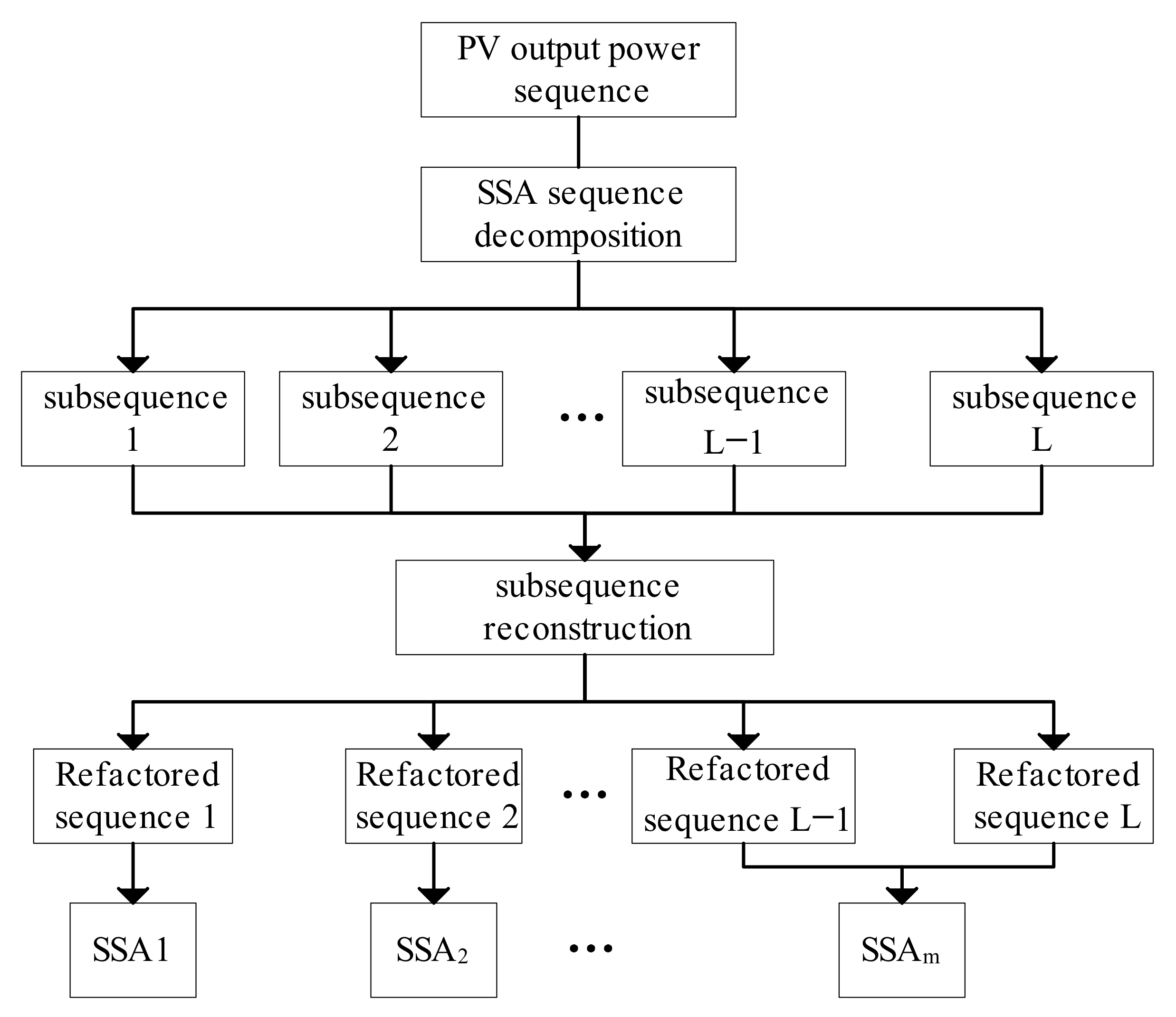
3.1. Singular Spectrum Analysis

SSA is an effective method that is used to analyze and predict nonlinear time series data, and its adaptive filtering property is suitable for dealing with data containing complex periodic components [41]. For PV power samples with volatility and nonlinear characteristics, SSA can decompose the original time series into several smoother series and build separate prediction models according to different volatility characteristics. The specific process is as follows.

3.1.1. Embedding

PV data are extracted with a sample size of N x = (x1, x2, …; xN); the length of the sequence is N (N > 2), the embedding dimensionality is set to L and the value range of L is usually an integer with 1 < L < N/2. The trajectory matrix G of L × K is generated, as shown in Equation (3).
G = G 1 , G 2 , , G K = x 1 x 2 x K x 2 x 3 x K + 1 x L x L + 1 x N
where the number of columns in G is expressed as K = N − L + 1.

3.1.2. Decomposition

Decomposition is performed on the trajectory matrix G, and the decomposition process is represented by Equation (4).
G = i = 1 e S i = i = 1 e λ i U i V i T
where e is the number of nonzero eigenvalues in the matrix GTG, and the eigenvalues are ranked from largest to smallest, i.e., λ 1 λ 2 λ e 0 ; λ i and the matrices U i and V i are called the eigentriad of the trajectory matrix G, where V i = G T U i λ i and U i is the eigenvector of eigenvalue λ i .

3.1.3. Reorganization

The above submatrices are filtered and reorganized to form p disjoint groups I = {i1, i2,…, ip}, as shown in Equation (5).
G I = S i 1 + S i 2 + + S i p

3.1.4. Diagonal Averaging
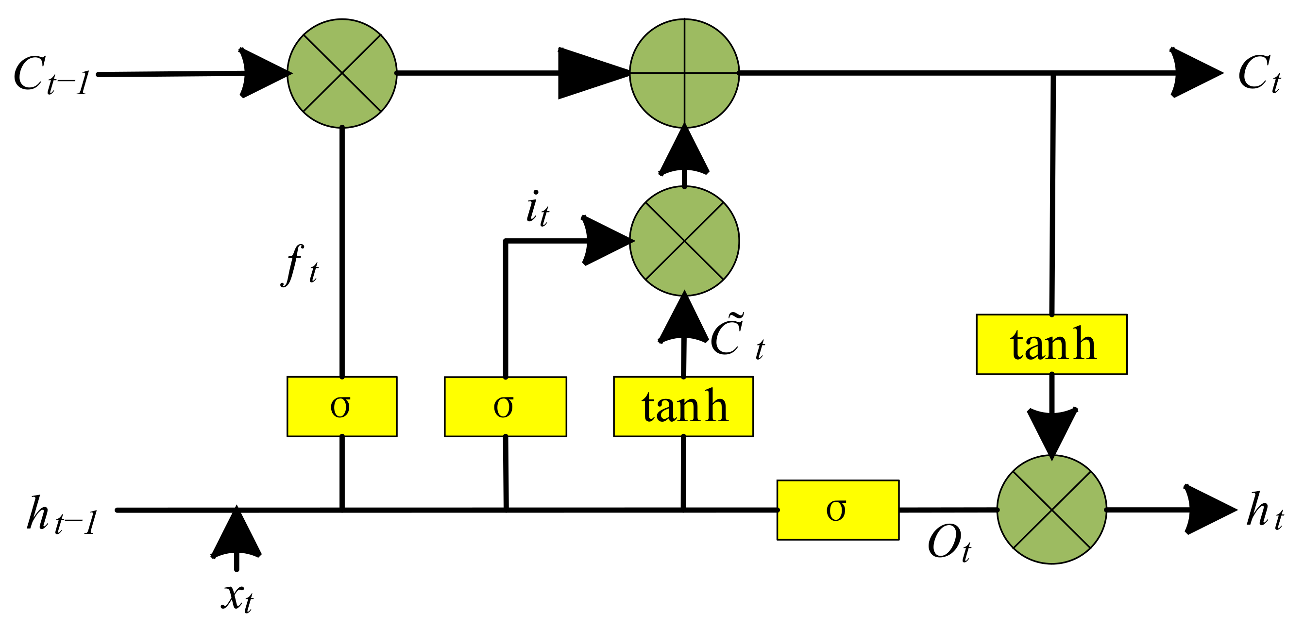
The purpose of diagonal averaging is to convert the above reorganization matrix into a time series. Let Y be a matrix of size L × K and x r s be a matrix element, where L* = min(L,K), K* = max(L,K), and N = L+K−1; when L < K, x r s = x r s ; that is, Y is converted into a time series y1, y2, y3, …; yN, and the formula is shown in Equation (6).
y k = 1 k k + 1 q = 1 x q , k q + 1 , 1 k L 1 L L p = 1 x q , k q + 1 , L < k K 1 N k + 1 N K + 1 p = k K + 1 x q , k q + 1 , K < k N
The SSA decomposition and reconstruction process is shown in Figure 2.
For a fluctuating PV power series, the choice of the embedding dimensionality L directly determines the performance of the model. The larger L is, the better it is at extracting the PV power components with regular periodic changes, and at the same time, the model generates redundant components; a smaller embedding dimensionality can effectively reflect the fluctuating dynamics of the given PV power series, but its ability to mine key information is limited. Therefore, L is generally set based on the periodicity of the data. For a PV output power series with short-time-scale fluctuation characteristics and long-time-scale variation trends, L must be reasonably selected. In this paper, when selecting the L value, the results are continuously compared through experiments. In the end, the best results are achieved when L is set to 13.

3.2. LSTM

LSTM is widely used in prediction problems. It is a special RNN model that can learn long-term data changes during model training. The LSTM prediction model completes the prediction task by controlling the information retention process through a forgetting gate, an input gate controlling the input information, and an output gate controlling the output information [42]. By controlling the memory unit at each time step, LSTM determines the amount of information to be transmitted at the next moment and the amount of information retained at the previous moment, so it can effectively capture the continuity of PV output power. Its structure is shown in Figure 3.
The structure contains a forgetting gate ft, an input gate it and an output gate Ot. The forgetting gate is able to selectively retain information in Ct−1; the input gate determines the amount of information preserved in Ct by the input Xt; and the output gate controls the effect of long-term memory on the current output ht. The expression is shown in Equation (7).
f t = σ W f h t 1 , x t + b f i t = σ W i h t 1 , x t + b i O t = σ W o h t 1 , x t + b o C t = tanh W c h t 1 , x t + b c C t = f t C t 1 + C t h t = O t tanh C t
where Wf, Wi, Wo and Wc are weight matrices; bf, bi, bo and bc are bias parameters; σ is the activation function; tanh is the hyperbolic tangent function; and ht−1 and Ct denote the previous cell output and internal candidate cell state, respectively. The LSTM network structure determines that the error does not decay sharply as the number of learning layers increases. At the same time, the network can solve the gradient explosion and gradient disappearance problems that may occur during training. Compared with shallow learning algorithms, LSTM exhibits an obvious advantage [43].

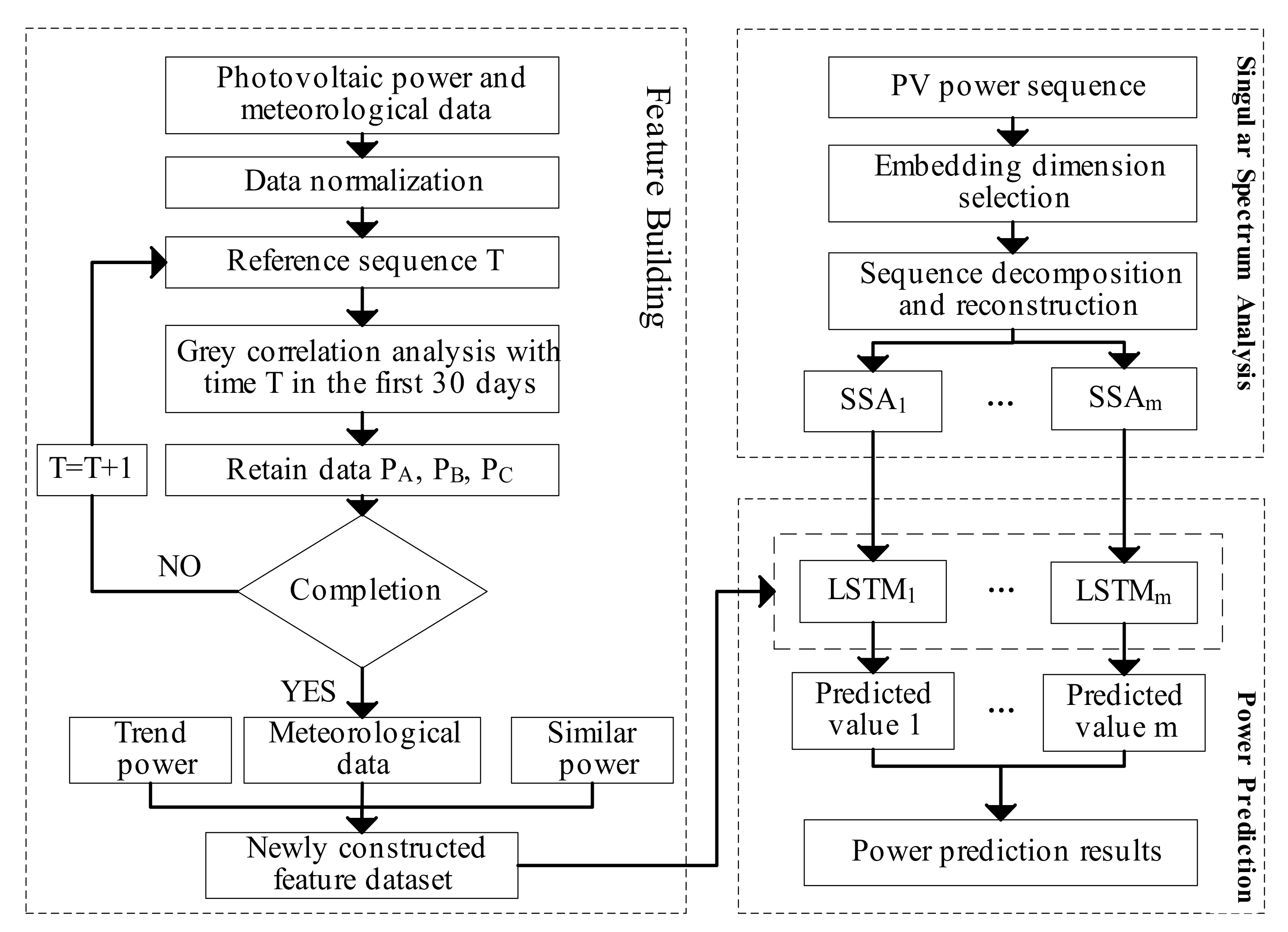
3.3. SSA-LSTM Prediction Model

For the PV power prediction problem, which possesses high volatility and stochasticity, this paper proposes a PV power prediction method considering feature-matched SSA and LSTM networks. The basic framework is shown in Figure 4.
The above steps include the LSTM time series prediction model and the LSTM prediction model containing the feature vector. The PV output power sequence is analyzed by SSA, the embedding dimensionality L is determined and the PV output power sequence is decomposed into L subsequences. The sequence reconstruction is performed according to the contribution degrees of the different subsequences to generate m SSA sequences. A corresponding LSTM prediction model is constructed for each SSA sequence, the power prediction process is carried out separately in the two prediction models and the final prediction result is obtained by superimposing the predicted power of each series. To adjust the parameters of the LSTM, this paper uses the GridSearchCV method. After setting the parameter range, this approach can automatically match the optimal optimization parameters for each LSTM model, enabling it to quickly optimize the parameters and reduce the operation time.

4. Case Study

4.1. Data Preparation

The simulation data in this paper are obtained from PV power and climate feature sequence samples collected from 1 June 2020 to 31 July 2020 in a domestic PV power plant, and each sample point contains 10 items: power, irradiance, humidity, ambient temperature, plate temperature and the newly constructed power features. The article data are selected from 5:00 a.m. to 18:45 p.m. which is defined as the effective power output period, with a total of 56 data points per day and a sampling interval of 15 min. The sample ratio of the training set to the test set is 8:2. All models in this paper are implemented using the Python programming language, TensorFlow is used to build a deep learning model, and sklearn’s GridSearchCV is used to realize parameter optimization [44]. The optimal hyperparameter configuration is crucial to the prediction performance. In this paper, the search ranges for the batch size and number of epochs are set in advance, and the search range is defined again based on the optimal output parameters until the optimal result is obtained. The loss function adopts the mean square error (mse), and Adam is used for training to prevent overfitting.

4.2. Error Analysis and Comparison

In this paper, the mean absolute error (MAE), root mean square error (RMSE) and coefficient of determination (R2) are used as the error indicators of photovoltaic power station output prediction. Although the mean absolute percentage error (MAPE) is widely used in experiments, its results are asymmetric. That is, errors higher than the original value will lead to greater absolute percentage errors [45]. The MAE, RMSE and R2 are calculated as follows:
M A E = 1 N i = 1 N P Pi P Mi
R M S E = 1 N N i = 1 P M i P P i 2
R 2 = 1 N i = 1 P P i P M i 2 N i = 1 P ¯ M P M i 2
where N is the number of predicted data points, and the time interval between each pair of data points is 15 min; PMi and Ppi are the actual output power and predicted power at prediction point i, respectively; and P ¯ M is the average of the actual power values of all samples.

4.3. Result and Discussion

First, SSA decomposition is performed on the PV output sequence, which is decomposed into 13 feature components, and principal component analysis is performed on the components. The results are shown in Figure 5.
It can be seen that: the contributions of the components decrease in order; the first component has a much higher contribution than the others; the contribution values of components two and three are basically equal; and the first six components are the main components with a cumulative share of 90%. In most cases, feature component screening causes a decrease in prediction performance [46], so all feature components are retained.
To verify the effectiveness of the SSA-LSTM prediction model, the results in this paper are compared with those of an LSTM network without the SSA decomposition model, as well as the XGBoost model. At the same time, we will evaluate the performance based on two frameworks: first, a univariate model using only time and historical load data, and second, a multivariate model incorporating feature data to better verify the importance of feature variables. The test set prediction results are shown in Table 5.
From the univariate experiments, it can be seen that the SSA-LSTM model has the best prediction effect compared to those of the XGBoost and LSTM models without SSA. The MAE is reduced by 65.5% and 54.8%, the RMSE is reduced by 74.3% and 62.5%, and the R2 is improved by 10.2% and 4.1%, respectively. This shows that the SSA can smooth the outgoing power series, which in turn improves the prediction results.
After adding the feature data, the prediction effects of the multivariate models are all significantly improved. Compared with the univariate models, the MAE and RMSE are reduced, respectively, by 41.3% and 36.1% for XGBoost; 42.3% and 50.2% for the LSTM model; and 49.4% and 45.4% for the SSA-LSTM. The prediction accuracy is further improved after incorporating the constructed feature, but the accuracy achieved by the LSTM model after incorporating the features is still inferior to that of the univariate SSA-LSTM model, indicating that the singular spectrum decomposition process plays an important role in the prediction procedure and proving the effectiveness of the SSA-LSTM model. It can be seen that in univariate prediction, the LSTM algorithm is more sensitive to seasonality and data trend [47], and singular universal analysis can highlight this characteristic in time series decomposition. Thus, the SSA-LSTM univariate model can achieve an excellent prediction effect. The smooth output sequence can also improve the prediction accuracy of the multivariable prediction model, which proves the effectiveness of the SSA-LSTM model.
To test the applicability of the model for prediction under complex weather conditions, three days with large fluctuations are selected from the dataset for output prediction, as shown in Figure 6. Since the prediction performances of the multivariate models in the above experiments are all better than those of the univariate models, multivariate models are used for these experiments. In the above experiments, the prediction accuracy of the XGBoost model is not as good as that of the LSTM model. Therefore, the XGBoost algorithm will be abandoned in the following experiments, and the SSA-LSTM model characterized by meteorological data will be used as a replacement to verify the role of the newly constructed power features. The models are classified into three categories: A, B and C. Among them, model A is the LSTM model using only meteorological data as its features. Model B is the SSA-LSTM model, which also uses only meteorological data as its features. Model C is an SSA-LSTM model with meteorological features and the new power features as its features, and the experimental results are as follows.
From the simulation results in Figure 6, it can be concluded that the curve fit of model C is the highest and the prediction accuracy is significantly improved over that of models A and B. The specific experimental results are shown in Table 6.
By comparing the error evaluation indices of model A and model B, it is seen that the prediction accuracy of the LSTM model is significantly improved after adding SSA decomposition, with MAE reductions of 70.5%, 75.1% and 85.2%, respectively; RMSE reductions of 72.7%, 74.8% and 71.7%, respectively; and significant R2 improvements, which fully verifies the effectiveness of the SSA model applied to LSTM. In addition, the prediction accuracy of model C is improved once again on the basis of model B, and the accuracy remains high under fluctuating weather conditions, which proves the effectiveness of the newly constructed features.
The results are compared and analyzed in Table 5 and Table 6. From the comparison results of model A and multivariate LSTM, it can be seen that after adding new features, the MAE and RMSE indicators decrease, and the R2 indicator improves significantly. This shows that the new features can effectively improve the prediction accuracy of the LSTM model. Therefore, after the above analysis, we believe that the new features and SSA can effectively improve the prediction accuracy of the model when they act on the LSTM model alone. Compared with the multivariate SSA-LSTM model, the prediction accuracy of model C is slightly lower. Because weather with strong volatility is more difficult to predict, it is easy to cause the accuracy of the prediction model to decline. The same problem arises in [37]. Secondly, when making single-day predictions, only the data before the prediction day can be selected as a training set, and the reduction of the training sample size will cause the prediction accuracy to decrease.
To better reflect the differences between the models, and at the same time verify the re-liability of the prediction models, residual analysis is conducted on the prediction results shown in Figure 6, and the specific results are shown in Figure 7. One column represents the test results for the same day, and the same row represents the same prediction model. From the figure, we can see that after adding the SSA decomposition model, the LSTM error range is significantly reduced. At the same time, it can be seen from the figure that the residual values are randomly distributed on both sides of the zero line, and there is no obvious trend and regularity, which verifies the reliability of the model.

5. Conclusions

In this paper, we propose a short-term PV prediction model based on feature matching (SSA-LSTM) by combining collected PV power generation data with PV power generation patterns observed under different climatic conditions; through example simulations, we can see the following:
(1)
Through the SSA decomposition method, the original high volatility and stochastic PV power output curve is decomposed into a series of smoother subsequences, which makes PV power prediction under fluctuating weather conditions much less difficult and improves the resulting prediction accuracy;
(2)
A reasonable feature selection process can highlight the key features of the input data, and the dataset obtained after feature matching can effectively improve the model prediction accuracy;
(3)
In an experimental results comparison, this paper adopts comparison tests between single-input models and multi-input models to evaluate the integrated prediction accuracy, and the results show that the SSA-LSTM prediction effect achieved after incorporating the new features is optimal.

Author Contributions

Conceptualization, Z.H. and J.H.; methodology, J.H. and J.M.; software, J.H. and J.M.; validation, Z.H., J.H. and J.M.; formal analysis, J.H.; investigation, J.H.; resources, J.H.; data curation, J.H.; writing—original draft preparation, J.H.; writing—review and editing, Z.H.; visualization, J.H.; supervision, Z.H.; project administration, J.H.; All authors have read and agreed to the published version of the manuscript.

Funding

This research received no external funding.

Data Availability Statement

Data are included in the article.

Conflicts of Interest

The authors declare no conflict of interest.

References

  1. Renewable Power Generation Costs in 2019. 2020. Available online: https://www.irena.org/publications/2020/Jun/Renewable-Power-Costs-in-2019 (accessed on 20 August 2022).
  2. IRENA. Future of Solar Photovoltaic: Deployment, Investment, Technology, Grid Integration and Socio-Economic Aspects (A Global Energy Transformation: Paper); International Renewable Energy Agency: Abu Dhabi, United Arab Emirates, 2019. [Google Scholar]
  3. Blaga, R.; Sabadus, A.; Stefu, N.; Dughir, C.; Paulescu, M.; Badescu, V. A current perspective on the accuracy of incoming solar energy forecasting. Prog. Energy Combust. Sci. 2019, 70, 119–144. [Google Scholar] [CrossRef]
  4. Turchenko, V.A.; Trukhanov, S.V.; Kostishin, V.G.; Damay, F.; Porcher, F.; Klygach, D.S.; Vakhitov, M.G.; Lyakhov, D.; Michels, D.; Bozzo, B.; et al. Features of structure, magnetic state and electrodynamic performance of SrFe12−xInxO19. Sci. Rep. 2021, 11, 18342. [Google Scholar] [CrossRef] [PubMed]
  5. Kozlovskiy, A.L.; Alina, A.; Zdorovets, M.V. Study of the effect of ion irradiation on increasing the photocatalytic activity of WO3 microparticles. J. Mater. Sci. Mater. Electron. 2021, 32, 3863–3877. [Google Scholar] [CrossRef]
  6. Kozlovskiy, A.L.; Shlimas, D.I.; Zdorovets, M.V. Synthesis, structural properties and shielding efficiency of glasses based on TeO2-(1-x) ZnO-xSm2O3. J. Mater. Sci. Mater. Electron. 2021, 32, 12111–12120. [Google Scholar] [CrossRef]
  7. Almessiere, M.A.; Algarou, N.A.; Slimani, Y.; Sadaqat, A.; Baykal, A.; Manikandan, A.; Trukhanov, S.V.; Trukhanov, A.V.; Ercan, I. Investigation of exchange coupling and microwave properties of hard/soft (SrNi0. 02Zr0. 01Fe11. 96O19)/(CoFe2O4) x nanocomposites. Mater. Today Nano 2022, 18, 100186. [Google Scholar] [CrossRef]
  8. Zambrano, A.F.; Giraldo, L.F. Solar irradiance forecasting models without on-site training measurements. Renew. Energy 2020, 152, 557–566. [Google Scholar] [CrossRef]
  9. Dorado-Moreno, M.; Navarin, N.; Gutiérrez, P.A.; Prieto, L.; Sperduti, A.; Salcedo-Sanz, S.; Hervás-Martínez, C. Multi-task learning for the prediction of wind power ramp events with deep neural networks. Neural Netw. 2020, 123, 401–411. [Google Scholar] [CrossRef]
  10. Aslam, M.; Lee, J.-M.; Kim, H.-S.; Lee, S.-J.; Hong, S. Deep learning models for long-term solar radiation forecasting considering microgrid installation: A comparative study. Energies 2019, 13, 147. [Google Scholar] [CrossRef] [Green Version]
  11. Rana, M.; Rahman, A. Multiple steps ahead solar photovoltaic power forecasting based on univariate machine learning models and data re-sampling. Sustain. Energy Grids Netw. 2020, 21, 100286. [Google Scholar] [CrossRef]
  12. Al-Dahidi, S.; Ayadi, O.; Adeeb, J.; Louzazni, M. Assessment of artificial neural networks learning algorithms and training datasets for solar photovoltaic power production prediction. Front. Energy Res. 2019, 7, 130. [Google Scholar] [CrossRef]
  13. Buwei, W.; Jianfeng, C.; Bo, W.; Shuanglei, F. A solar power prediction using support vector machines based on multi-source data fusion. In Proceedings of the 2018 International Conference on Power System Technology (POWERCON), Guangzhou, China, 6–8 November 2018; pp. 4573–4577. [Google Scholar]
  14. Ahmad, M.W.; Mourshed, M.; Rezgui, Y. Tree-based ensemble methods for predicting PV power generation and their comparison with support vector regression. Energy 2018, 164, 465–474. [Google Scholar] [CrossRef]
  15. Fan, J.; Wu, L.; Ma, X.; Zhou, H.; Zhang, F. Hybrid support vector machines with heuristic algorithms for prediction of daily diffuse solar radiation in air-polluted regions. Renew. Energy 2020, 145, 2034–2045. [Google Scholar] [CrossRef]
  16. Munawar, U.; Wang, Z. A framework of using machine learning approaches for short-term solar power forecasting. J. Electr. Eng. Technol. 2020, 15, 561–569. [Google Scholar] [CrossRef]
  17. Andrade, J.R.; Bessa, R.J. Improving renewable energy forecasting with a grid of numerical weather predictions. IEEE Trans. Sustain. Energy 2017, 8, 1571–1580. [Google Scholar] [CrossRef] [Green Version]
  18. LeCun, Y.; Bengio, Y.; Hinton, G. Deep learning. Nature 2015, 521, 436–444. [Google Scholar] [CrossRef]
  19. Sun, Y.; Venugopal, V.; Brandt, A.R. Short-term solar power forecast with deep learning: Exploring optimal input and output configuration. Sol. Energy 2019, 188, 730–741. [Google Scholar] [CrossRef]
  20. Ghimire, S.; Deo, R.C.; Raj, N.; Mi, J. Deep learning neural networks trained with MODIS satellite-derived predictors for long-term global solar radiation prediction. Energies 2019, 12, 2407. [Google Scholar] [CrossRef] [Green Version]
  21. Zhang, C.; Liang, M.; Song, X.; Liu, L.; Wang, H.; Li, W.; Shi, M. Generative adversarial network for geological prediction based on TBM operational data. Mech. Syst. Signal Processing 2020, 162, 108035. [Google Scholar] [CrossRef]
  22. Zhang, J.; Verschae, R.; Nobuhara, S.; & Lalonde, J.F. Deep photovoltaic nowcasting. Sol. Energy 2018, 176, 267–276. [Google Scholar] [CrossRef] [Green Version]
  23. Qing, X.; Niu, Y. Hourly day-ahead solar irradiance prediction using weather forecasts by LSTM. Energy 2018, 148, 461–468. [Google Scholar] [CrossRef]
  24. He, W. Load forecasting via deep neural networks. Procedia Comput. Sci. 2017, 122, 308–314. [Google Scholar] [CrossRef]
  25. Taieb, S.B.; Bontempi, G.; Atiya, A.F.; Sorjamaa, A. A review and comparison of strategies for multi-step ahead time series forecasting based on the NN5 forecasting competition. Expert Syst. Appl. 2012, 39, 7067–7083. [Google Scholar] [CrossRef] [Green Version]
  26. Santhosh, M.; Venkaiah, C.; Kumar, D.V. Short-term wind speed forecasting approach using ensemble empirical mode decomposition and deep Boltzmann machine. Sustain. Energy Grids Netw. 2019, 19, 100242. [Google Scholar] [CrossRef]
  27. Wang, L.; Li, X.; Bai, Y. Short-term wind speed prediction using an extreme learning machine model with error correction. Energy Convers. Manag. 2018, 162, 239–250. [Google Scholar] [CrossRef]
  28. Golyandina, N.; Nekrutkin, V.; Zhigljavsky, A.A. Analysis of Time Series Structure: SSA and Related Techniques; CRC Press: Boca Raton, FL, USA, 2001. [Google Scholar]
  29. Broomhead, D.S.; King, G.P. Extracting qualitative dynamics from experimental data. Phys. D Nonlinear Phenom. 1986, 20, 217–236. [Google Scholar] [CrossRef]
  30. Moreno, S.R.; dos Santos Coelho, L. Wind speed forecasting approach based on singular spectrum analysis and adaptive neuro fuzzy inference system. Renew. Energy 2018, 126, 736–754. [Google Scholar] [CrossRef]
  31. Liu, H.; Mi, X.; Li, Y.; Duan, Z.; Xu, Y. Smart wind speed deep learning based multi-step forecasting model using singular spectrum analysis, convolutional Gated Recurrent Unit network and Support V ector Regression. Renew. Energy 2019, 143, 842–854. [Google Scholar] [CrossRef]
  32. Wang, C.; Zhang, H.; Ma, P. Wind power forecasting based on singular spectrum analysis and a new hybrid Laguerre neural network. Appl. Energy 2020, 259, 114139. [Google Scholar] [CrossRef]
  33. Moreno, S.R.; da Silva, R.G.; Mariani, V.C.; dos Santos Coelho, L. Multi-step wind speed forecasting based on hybrid multi-stage decomposition model and long short-term memory neural network. Energy Convers. Manag. 2020, 213, 112869. [Google Scholar] [CrossRef]
  34. Chen, C.; Duan, S.; Cai, T.; Liu, B. Online 24-h solar power forecasting based on weather type classification using artificial neural network. Sol. Energy 2011, 85, 2856–2870. [Google Scholar] [CrossRef]
  35. Wang, F.; Zhen, Z.; Wang, B.; Mi, Z. Comparative study on KNN and SVM based weather classification models for day ahead short term solar PV power forecasting. Appl. Sci. 2017, 8, 28. [Google Scholar] [CrossRef] [Green Version]
  36. Lin, P.; Peng, Z.; Lai, Y.; Cheng, S.; Chen, Z.; Wu, L. Short-term power prediction for photovoltaic power plants using a hybrid improved Kmeans-GRA-Elman model based on multivariate meteorological factors and historical power datasets. Energy Convers. Manag. 2018, 177, 704–717. [Google Scholar] [CrossRef]
  37. Gu, B.; Shen, H.; Lei, X.; Hu, H.; Liu, X. Forecasting and uncertainty analysis of day-ahead photovoltaic power using a novel forecasting method. Appl. Energy 2021, 299, 117291. [Google Scholar] [CrossRef]
  38. Zhang, N.; Ren, Q.; Liu, G.; Guo, L.; Li, J. Short-term PV Output Power Forecasting Based on CEEMDAN-AE-GRU. J. Electr. Eng. Technol. 2022, 17, 1183–1194. [Google Scholar] [CrossRef]
  39. Nam, K.; Hwangbo, S.; Yoo, C. A deep learning-based forecasting model for renewable energy scenarios to guide sustainable energy policy: A case study of Korea. Renew. Sustain. Energy Rev. 2020, 122, 109725. [Google Scholar] [CrossRef]
  40. Taiyangshan, W. Wuzhong Taiyangshan PV Power Station Annual Report; Taiyangshan Photovoltaic Power Station: WuZhong, China, 2016. [Google Scholar]
  41. Rocco, S.C.M. Singular spectrum analysis and forecasting of failure time series. Reliab. Eng. Syst. Saf. 2013, 114, 126–136. [Google Scholar] [CrossRef]
  42. Tan, M.; Yuan, S.; Li, S.; Su, Y.; Li, H.; He, F. Ultra-short-term industrial power demand forecasting using LSTM based hybrid ensemble learning. IEEE Trans. Power Syst. 2019, 35, 2937–2948. [Google Scholar] [CrossRef]
  43. Bianchi, F.M.; Maiorino, E.; Kampffmeyer, M.C.; Rizzi, A.; Jenssen, R. Recurrent Neural Networks for Short-Term Load Forecasting: An Overview and Comparative Analysis; Springer: Cham, Switzerland, 2017. [Google Scholar]
  44. Hutter, F.; Kotthoff, L.; Vanschoren, J. Automated Machine Learning: Methods, Systems, Challenges; Springer Nature: Berlin/Heidelberg, Germany, 2019; pp. 7–8, 219. [Google Scholar]
  45. Makridakis, S. Accuracy measures: Theoretical and practical concerns. Int. J. Forecast. 1993, 9, 527–529. [Google Scholar] [CrossRef]
  46. Stratigakos, A.; Bachoumis, A.; Vita, V.; Zafiropoulos, E. Short-Term Net Load Forecasting with Singular Spectrum Analysis and LSTM Neural Networks. Energies 2021, 14, 4107. [Google Scholar] [CrossRef]
  47. Bandara, K.; Bergmeir, C.; Hewamalage, H. LSTM-MSNet: Leveraging forecasts on sets of related time series with multiple seasonal patterns. IEEE Trans. Neural Netw. Learn. Syst. 2020, 32, 1586–1599. [Google Scholar] [CrossRef]
Figure 1. Typical weather-PV output power curves. (a) Typical weather for sunny days (b) Typical weather for partly cloudy days (c) Typical weather for cloudy days (d) Typical weather for rainy days.
Energies 15 07806 g001
Figure 2. Flowchart of the SSA model.
Energies 15 07806 g002
Figure 3. LSTM cell structure diagram.
Energies 15 07806 g003
Figure 4. Flowchart of the combined forecasting model.
Energies 15 07806 g004
Figure 5. SSA and principal component analysis.
Energies 15 07806 g005
Figure 6. Forecasting results: (a) is the forecast result on 5 July, (b) is the forecast result on 7 July and (c) is the forecast result on 10 July.
Energies 15 07806 g006
Figure 7. Prediction residual plot.
Energies 15 07806 g007
Table 1. Correlation coefficients for the first 7 moments.
Timet−1t−2t−3t−4t−5t−6t−7
Correlation coefficient0.950.920.880.850.810.760.71
Table 2. Similarity feature selection process.
Input: PV output power history dataset.
1. The process of data normalization;
2. Select the PV outputs at time t as the reference series;
3. Perform grey relation analysis with each t-moment for the previous 30 days;
4. Sort r values from largest to smallest, and retain the powers of the three moments with the strongest correlations;
5. t moments +1, and repeat steps 2–4 until the last data point is reached;
Output: PV power, Pa, Pb, Pc, complete feature construction.
Table 3. Correlation coefficient.
FeaturesGHIATCTRHt−1t−2t−3PaPbPc
Power0.7960.5030.273−0.0080.9420.9140.8780.9170.6070.585
Table 4. PV output features.
Serial NumberFeatureSerial NumberFeature
1Global horizontal irradiance6Power at moment t−2
2Ambient temperature7Power at moment t−3
3Component temperature8Similar power Pa
4Relative humidity9Similar power Pb
5Power at moment t−110Similar power Pc
Table 5. PV output forecasting results.
Prediction MethodUnivariateMultivariate
MAE/MWRMSE/MWR2MAE/MWRMSE/MWR2
XGBoost5.1217.8450.9013.0035.0180.959
LSTM3.9135.3740.9532.2562.6720.988
SSA-LSTM1.7652.0100.9930.8921.0960.998
Table 6. Error evaluation indices of each prediction model.
Forecasting DatePredictive ModelsMAE/MWRMSE/MWR2
July 5thA3.9465.4520.523
B1.1631.4860.964
C1.0641.3810.969
July 7thA8.58011.9790.626
B2.1373.0100.976
C1.7782.4110.984
July 10thA6.80110.150.722
B2.0382.8630.977
C2.0172.5400.982
Publisher’s Note: MDPI stays neutral with regard to jurisdictional claims in published maps and institutional affiliations.

