Standing Wave Pattern and Distribution of Currents in Resonator Arrays for Wireless Power Transfer

Abstract

The possibility of increasing the transmission efficiency in mid-range wireless power transfer (WPT) applications can be achieved by inserting resonant relay coils between the transmitting and receiving sides of the device, forming an array of magnetically coupled resonant circuits, over which a receiver can be placed. This is a very cheap solution for improving the performance of the WPT apparatus, even if the complexity of the system increases, requiring a complete and detailed investigation for a smart design and control of the apparatus. The presented study investigates the current distribution in the coils of the array, which revealed strong peaks in magnitude depending on the load and receiver position. The analysis is carried out with the transmission line (TL) theory and it is performed for different positions of the receiver, as well as for different load conditions. Furthermore, a real application is considered and discussed, which includes the presence of a power converter as power supply and a battery charging system as load. Each resonant circuit resonates at 150 kHz and the whole apparatus is capable to transmit power up to 1 kW with an efficiency around $70\%$. The theoretical results have been validated with experimental measurements.

1. Introduction

In recent years, wireless power transfer (WPT) has received increasing attention for the prospects of use that it offers, ranging from powering portable electronic devices to electric vehicle (EV) charging. The WPT systems are continuously improved, allowing more power to be transferred and operation in difficult environment, where water, dirt or dust are present. The major limitations for inductive power transfer (IPT) technologies are the magnetic field generated that can cause disturbances to electric and/or electronic devices and field exposure to people in the surroundings as well as the transmission distance, which is limited by the nature of the physical phenomena exploited. As a consequence, these issues have become the most important challenges in this field and different solutions have been proposed in the literature [1,2,3,4,5]. It is indeed necessary to consider both problems when realizing WPT devices. High-frequency IPT systems are usually the most popular candidates, allowing the size of the components to be limited with an acceptable transmission distance, even if the electromagnetic radiation may become hazardous as the frequency increases. For this reason, they can be sized for a limited amount of power, resulting in WPT systems suitable for portable electronics or medical devices only [6,7]. Another widespread alternative is represented by the possibility of inserting relay coils between the transmitting and receiving circuits, thereby forming a structure of magnetically coupled resonators as shown in Figure 1. In this case, the power rating of the apparatus is determined by the size of the coils and related components, which can be tailored also for high power transfer, as it is needed in industry or EV charging applications. There are many papers that testify the potential of relay coils, arranged in widely differing ways, as reported in [5,8,9,10,11,12,13,14], even if a conventional structure and arrangement of the coils is not discussed.

Configuring the system as presented in [14,15,16], an array of resonant magnetically coupled circuits is formed, with the possibility of placing a receiver over it and then make the power transmission very tolerant to the receiver misalignment without the addition of complex power electronic circuits. This peculiarity makes resonator arrays for IPT applications a very cheap and simple solution.

However, the interaction between the coils leads to power-reflection phenomena which, in turn, alter the current distribution in the windings, causing strong peaks in some of the resonators and the strong increase in the magnitude of the current can lead to severe overloads in the resonator windings, with a non-negligible thermal stress. Furthermore, the raised current increases the Joule losses in the coils, with consequent efficiency decrease. It is important to notice that the resonators operate in resonance, meaning that the current is limited by the resistance of the wire only, which should be kept very small in order to avoid important losses. It is easy to understand that the monitoring of the standing wave phenomenon is crucial to avoid system breakdown and it should be performed both in the design and operating stages. These phenomena are investigated and discussed in this paper, carrying out the analysis first with Kirchhoff voltage law (KVL) equations [17,18] and then through the theory of magneto-inductive (MI) waves [19,20,21] that is exploited in order to provide a satisfactory description of the operation and useful insights into the design. The efficiency of this kind of systems has been deeply investigated [12,16,18,21], while the behaviour of the resonator currents requires a more in-depth research due to power reflection phenomena that can occur [21]. The main aim of this work is to analyse the behaviour of the array currents considering a real load and power source, and to present a mathematical model capable of describing the phenomena that govern the operation of resonator arrays, in case of practical implementations.

The manuscript is organized as follows. In Section 2, the structure of the proposed array of resonators is described, with the description of two different approaches for its analysis. Then, Section 3 is focused on the equivalent circuit model of the apparatus—including also the power source and the load—and, in Section 4, the problem of the current peaks in the resonators is theoretically and numerically investigated. The study is extended to the case of arrays of resonators employed as transmitting devices in Section 5. The theoretical and numerical analyses have been experimentally verified in Section 6. Finally, Section 7 concludes the paper discussing and summarising the achieved results.

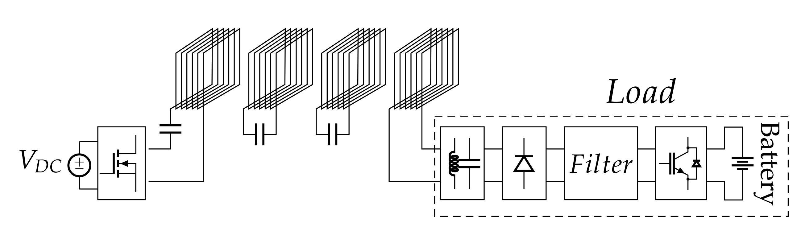
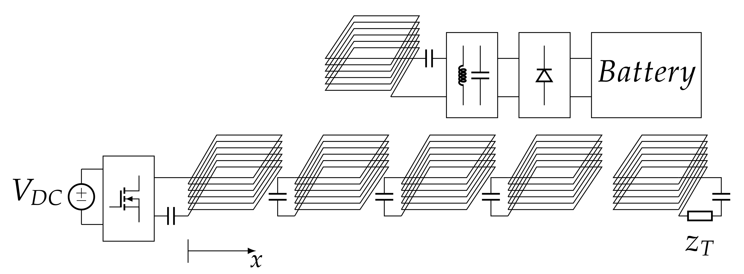
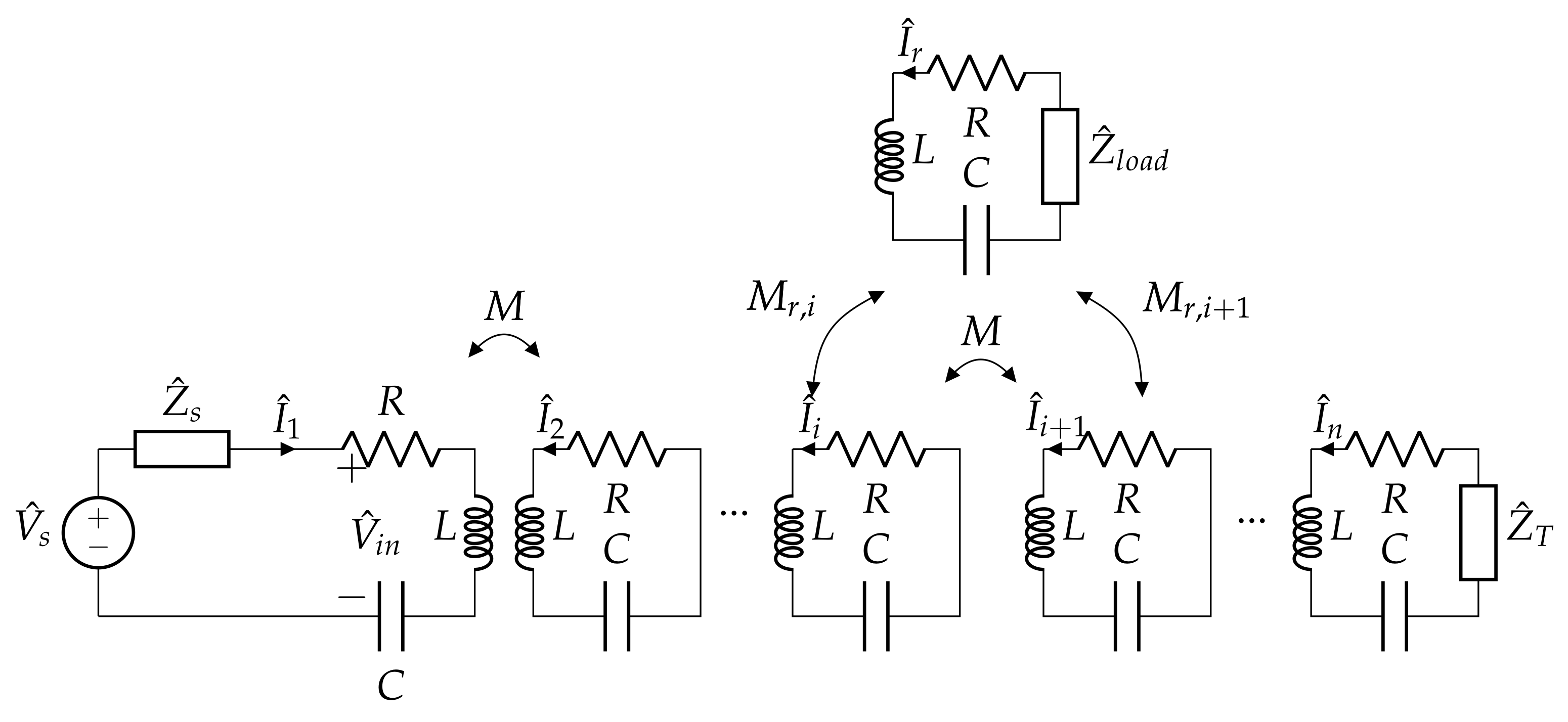
2. Resonator Array for IPT

The WPT system considered in this work consists of an array of n identical $L-C$ series resonant circuits, called resonators or cells, which are arranged in a plane along a line to form a 1-D structure and are magnetically coupled as shown in Figure 2. The resonators are spaced by the same distance and consequently each pair of adjacent resonators has the same mutual inductance M. In the following analysis, the mutual coupling between nonadjacent circuits is neglected, being much lower than that between adjacent cells. This hypothesis is called in literature “nearest neighbourhood interaction” [20] and it has been analytically and experimentally verified. Each resonator of intrinsic resistance R is tuned to a resonant frequency $f_0=1/\left(2\pi \sqrt{LC}\right)$, where L is the self-inductance of each resonator and C the capacitance of an additional capacitor connected in series to the resonator. The cell connected to the power source is labelled 1, whereas the last cell of the array is labelled n. It is important to highlight that this study considers the first harmonic of the electrical quantities voltage and current of a real IPT system. The power supply can be in general represented with its Thévenin equivalent circuit, then as an ideal voltage source with a series impedance that, at the resonant frequency $f_0$, can be named as ${\widehat{V}}_s$ and ${\widehat{Z}}_s$, respectively. The load is represented by the impedance ${\widehat{Z}}_T$ connected to the last resonator of the array.

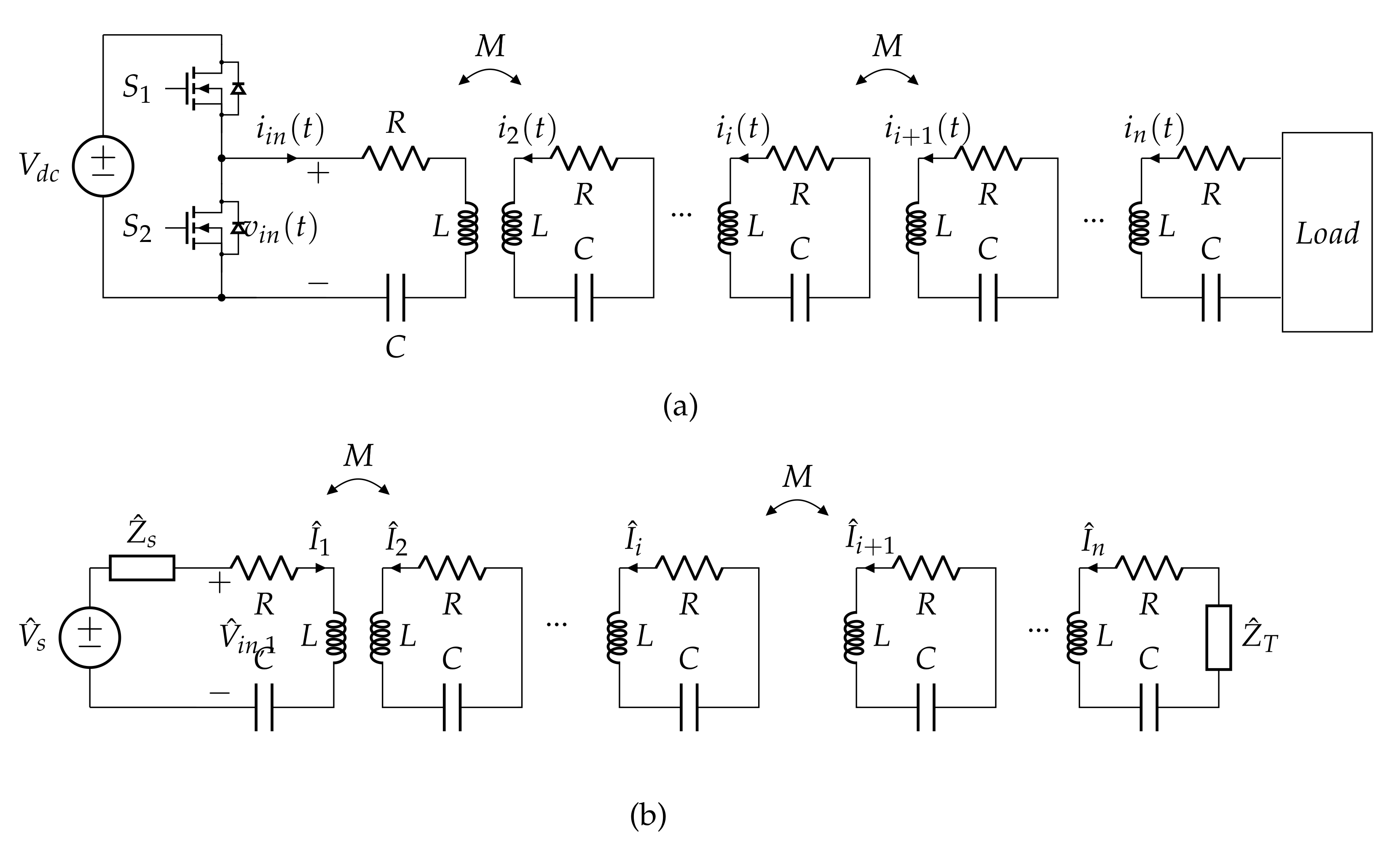
2.1. Circuit Analysis

The analysis is developed considering phasor quantities for the voltages and currents involved in the system, which can be determined solving the KVL equations written for each cell. This approach is the most common, and implies to solve the system

$$\widehat{\mathbf{I}}={\widehat{\mathbf{Z}}}_{\mathbf{m}}^{-1}\widehat{\mathbf{V}}$$

(1)

where $\widehat{\mathbf{V}}={[\widehat{V_s}0\dots 0]}^T$ is the phasor voltage vector (with $\widehat{V_s}$ the phasor supply voltage of the transmitter), $\widehat{\mathbf{I}}$ is the vector of the phasor currents flowing in the resonators and ${\widehat{\mathbf{Z}}}_{\mathbf{m}}$ is the impedance matrix of the array resonators. However, the circuit analysis, carried out through the solution of (1), is as simple as poor in content, since it does not suggest any motivation for the results that it provides.

2.2. Magneto-Inductive Waves

Alternatively, the array of resonators can be considered as a cascade connection of identical two-port networks, where each of them represents the coupling between adjacent resonators, phase shifting and attenuating the input current and voltage. In this paper a cascade of $n-1$ chain matrices ${\mathbf{T}}_{i,i+1}$ is used to represent an array of n cells. For two adjacent resonators i and $i+1$ the voltages and currents at the input and output ports of the two-port network are related by

$$\left[\begin{array}{c}{\widehat{V}}_i\\ {\widehat{I}}_i\end{array}\right]={\mathbf{T}}_{i,i+1}\left[\begin{array}{c}{\widehat{V}}_{i+1}\\ {\widehat{I}}_{i+1}\end{array}\right]$$

(2)

with

$${\mathbf{T}}_{i,i+1}=\left[\begin{array}{cc}{\widehat{A}}_{i,i+1}& {\widehat{B}}_{i,i+1}\\ {\widehat{C}}_{i,i+1}& {\widehat{D}}_{i,i+1}\end{array}\right]$$

(3)

where

$$\begin{array}{c}{\widehat{A}}_{i,i+1}=-\frac{{\widehat{Z}}_i}{{\widehat{Z}}_{M_{i,i+1}}}\\ {\widehat{B}}_{i,i+1}={\widehat{Z}}_{M_{i,i+1}}-\frac{{\widehat{Z}}_i{\widehat{Z}}_{i+1}}{{\widehat{Z}}_{M_{i,i+1}}}\\ {\widehat{C}}_{i,i+1}=-\frac{1}{{\widehat{Z}}_{M_{i,i+1}}}\\ {\widehat{D}}_{i,i+1}=-\frac{{\widehat{Z}}_{i+1}}{{\widehat{Z}}_{M_{i,i+1}}}\end{array}$$

(4)

For an array of identical resonators of impedance Z, ${\widehat{Z}}_i={\widehat{Z}}_{i+1}=\widehat{Z}/2$ and ${\widehat{Z}}_1={\widehat{Z}}_n=Z$, while the mutual impedance ${\widehat{Z}}_{M_{i,i+1}}=j\omega M$. Thus, the array can be described by three different ${\mathbf{T}}_{i,i+1}$ matrices only. In the following the transmission matrix associated to the two-port networks representing the coupling between two adjacent array resonators i and $i+1$ is simply named as $\mathbf{T}$, with the exception of the two matrices ${\mathbf{T}}_{1,2}$ and ${\mathbf{T}}_{n-1,n}$ of the two ports comprising the first and last resonators of the array, respectively. A similar structure can be associated to a TL able to support the propagation of a current wave which is called magneto-inductive (MI) wave in [19].

It must be clarified that MI waves, whose idea comes from the analysis of the array resonator currents, do not correspond to electromagnetic waves. Indeed, as all the cells of the array are magnetically coupled, in resonance the currents of adjacent resonators are displaced by 90 electrical degrees due to the mutual coupling ($j\omega M$). Thus, exciting the first array coil, a 90 degrees-displaced voltage (and then the corresponding current) is induced in the second resonator which, in turn, induces a voltage and then a current in the third one, and so on, until the last one. This behaviour mirrors the one of a wave that propagates in the space along the array. Thus, the considered structure is described in terms of the current circulating in each cell. A simple MI wave solution for a 1-D configuration according to [20,22] is:

$$\widehat{I_i}={\widehat{I}}_1{e}^{-\widehat{\gamma }(i-1)d}$$

(5)

where $\widehat{I_i}$ is the ith resonator phasor current and ${\widehat{I}}_1$ is the first resonator phasor current, d is the side-length of each resonator forming the array and $\widehat{\gamma }=\alpha +j\beta$ is the propagation constant, with $\alpha$ attenuation constant and $\beta$ phase constant. The attenuation per cell of the MI wave can be expressed as [16]:

$$\alpha d=sin{h}^{-1}\left(\frac{1}{kQ}\right)$$

(6)

where $k=2M/L$ is the coupling coefficient between adjacent cells and $Q={\omega }_{0}L/R$ the quality factor of the single cell, being ${\omega }_0=2\pi f_0$ the resonant angular frequency. The current wave attenuation is due to the resistance R of each cell and becomes stronger as the coupling between adjacent cells weakens. The propagation of MI waves is governed by the dispersion equation which in case of low losses gives the following simple relationship [16,20]:

$$cos\left(\beta d\right)=\left(\frac{{\omega }_0^2-{\omega }^2}{k{\omega }^2}\right)$$

(7)

which defines the frequency limits of the propagation band enforcing $\left|cos\right(\beta d\left)\right|=1$. When the system operates at ${\omega }_0$, the attenuation is minimized and the phase shift per cell is $\beta d=\pi /2$. It must be noticed that each resonator contributes with a phase shift of $\beta d$, meaning that the wavelength of the MI wave is fixed by the length d of the resonators and results ${\lambda }_{MIW}=4d$. The analogy with TLs also suggests the possibility of matching the MI waveguide, condition that avoids MI-standing waves. In matching condition and in resonance for a low-loss line, i.e., $R\ll {\omega }_{0}M$, the current has the same magnitude in all the array resonators and the power transferred to the terminal resonator is maximum [15,23]. This is possible if the array is terminated in a lumped impedance equal to the characteristic one of the MI waveguide, defined as [20]:

$${\widehat{Z}}_0=j\omega M{e}^{-\widehat{\gamma }d}.$$

(8)

For a low-loss MI waveguide, ${\widehat{Z}}_0$ simplifies to ${\widehat{Z}}_0\approx {\omega }_{0}M$ for $f=f_0$. The same result can be found considering the general representation of a transmission line segment of length d by means of a transmission matrix, which for a MI waveguide can be expressed as [24]

$${\mathbf{T}}_{MI-TL}=\left[\begin{array}{cc}cosh\left(\widehat{\gamma }d\right)& {\widehat{Z}}_{0}sinh\left(\widehat{\gamma }d\right)\\ \frac{1}{{\widehat{Z}}_0}sinh\left(\widehat{\gamma }d\right)& cosh\left(\widehat{\gamma }d\right)\end{array}\right].$$

(9)

By Equating (9) and (3) the characteristic impedance of the considered line segment is found as:

$${\widehat{Z}}_{0_{i,i+1}}=\sqrt{\frac{{\widehat{B}}_{i,i+1}}{{\widehat{C}}_{i,i+1}}}$$

(10)

which becomes ${\widehat{Z}}_0\approx {\omega }_{0}M$ for a low-loss array operating in resonance, being $Z_i=Z_{i+1}=R^2/4\approx 0$.

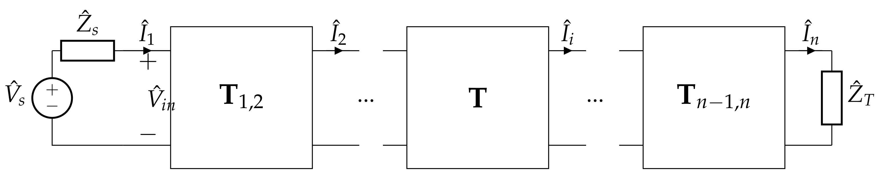
3. Array Circuit Modelling

Carrying out the study of resonator arrays with both the circuit theory and MI waves, it is required to evaluate all the parameters of the system, since they strongly affect the current distribution and the power transfer. In order to analyse the feasibility of a resonator array for WPT, possible applications with real power supplies and loads have to be considered; a precise analysis has to be carried out when dealing with this kind of apparatuses, since they usually present a nonlinear behaviour.

The power supply is assumed to be a half-bridge inverter and, thanks to the pass-band filter behaviour of the resonator array, it can be represented by means of first harmonic approximation through its equivalent Thévenin circuit, composed of an ideal voltage source ${\widehat{V}}_s$ with a series impedance ${\widehat{Z}}_s$. In particular, according to [14]

$${\widehat{V}}_s=\frac{2V_{dc}}{\pi }{e}^{j0}$$

(11)

where $V_{dc}$ is the bus DC voltage at the input side of the converter and

$${\widehat{Z}}_s=\frac{8R_{on}}{{\pi }^2}{e}^{j\frac{t_d{\omega }_0}{2}}$$

(12)

where $R_{on}$ is the resistance of the MOSFET. The term $t_d$ indicates the dead-time of the considered inverter. Usually, $t_d\ne 0$ and then the impedance ${\widehat{Z}}_s$ is complex, with an inductive behaviour. If the load is assumed to be a battery charging system, it can be described by its equivalent impedance ${\widehat{Z}}_{load}$, as reported in [14]. Then,

$${\widehat{Z}}_{load}=\frac{8}{{\pi }^2}{R}_{battery}$$

(13)

where $R_{battery}$ is the resistance of the battery pack. Considering loads different from the previous one, in the array represented in Figure 2b the impedance ${\widehat{Z}}_{load}$ corresponds to the termination impedance of the array ${\widehat{Z}}_T$.

The two impedances ${\widehat{Z}}_s$ and ${\widehat{Z}}_T$ depicted in Figure 2b are the two parameters that govern the reflections in the array and their different possible values are considered in the following.

4. Current Peaks and Standing Waves

As it has been introduced in Section 2, in case of mismatch of the termination impedance of the array, a standing wave pattern can occur for the MI wave. Thus, some resonators may experience very high currents, depending on the values of the impedance at the input and output sides of the array, as well as the length of the array. With the help of the theory of MI waves these phenomena can be rigorously described. In order to proceed with the analysis, the equivalent TL is defined as described in Section 2 and shown in Figure 3, where the input and termination of the array are modelled as illustrated in Section 3. According to the classic theory of the traditional TLs, it is possible to determine the current behaviour studying the propagation and reflections experienced at the two terminals. The first reflection that the current wave expressed by (5) undergoes is due to the mismatching of the termination impedance ${\widehat{Z}}_T$, which usually differs from the characteristic impedance ${\widehat{Z}}_0$. It is possible to define the termination reflection coefficient as:

$${\widehat{\rho }}_T=\frac{{\widehat{Z}}_T-{\widehat{Z}}_0}{{\widehat{Z}}_T+{\widehat{Z}}_0}.$$

(14)

Considering the internal impedance of the power source ${\widehat{Z}}_s$ as the the input impedance of the MI waveguide, the source reflection coefficient can be expressed as:

$${\widehat{\rho }}_s=\frac{{\widehat{Z}}_s-{\widehat{Z}}_0}{{\widehat{Z}}_s+{\widehat{Z}}_0}.$$

(15)

It can be observed that it is very difficult to realize the matching of the input port, too, being ${\widehat{Z}}_s$ dependent on the inverter components and control strategy.

The standing wave pattern is the result of multiple reflections between the input and termination sides of the line, whose interaction has been considered as an overlap of the various components. The final mathematical expression is given in [25] for waves in traditional TLs and a similar one can be obtained for MI waves. After some mathematical manipulation, the current in the ith resonator of the array can be expressed as:

$$\widehat{I_i}=\frac{{\widehat{V}}_s}{{\widehat{Z}}_s+{\widehat{Z}}_0}\frac{e^{-\widehat{\gamma }(i-1)d}-{\widehat{\rho }}_T{e}^{-2\widehat{\gamma }(n-1)d}{e}^{\widehat{\gamma }(i-1)d}}{1-{\widehat{\rho }}_S{\widehat{\rho }}_T{e}^{-2\widehat{\gamma }(n-1)d}}.$$

(16)

The consequence of the mismatching of both sides of the line is the interference between the reflected waves, with the consequent creation of a standing wave pattern for the current, which exhibits maxima and minima with a periodicity that depends on the wavelength of the individual wave. When a standing wave pattern occurs, the power transfer capability of the system is strongly reduced (the power is reflected) [16], even if the worst consequence is the stress of the electric and electronic components. According to [25], the usual procedure for the definition of the shape of this pattern can be achieved by specifying:

• The ratio of the current magnitude maximum to the minimum in the standing wave pattern (standing wave ratio);
• The location of any current minimum, with reference to a specified coordinate;
• The distance between two consecutive maxima or minima.

The standing wave ratio (SWR) is introduced in order to evaluate the magnitude of the wave peaks and is defined as

$$SWR=\frac{|{\widehat{I}}_i{|}_{\max }}{|{\widehat{I}}_i{|}_{\min }}$$

(17)

where $|{\widehat{I}}_i{|}_{\max }$ and $|{\widehat{I}}_i{|}_{\min }$ are the current magnitude maximum and minimum in the standing wave pattern, respectively.

The distance between consecutive current maxima or minima corresponds, as it is well known, to half wavelength. As the wavelength of an MI wave is ${\lambda }_{MIW}=4d$, it results in being $2d$. It must be noticed that, considering the attenuation due to the losses, the magnitude of the current peaks is expected to be lower as they occur far from the power supply.

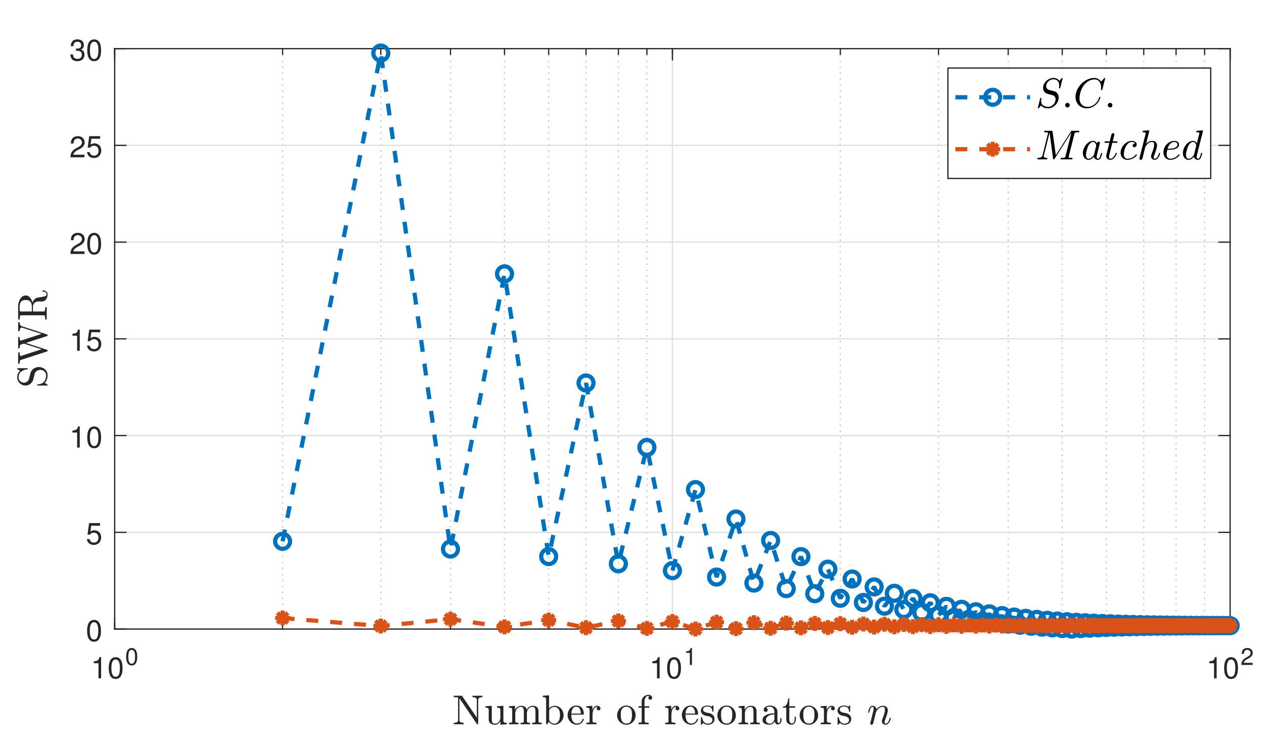
4.1. Numerical Analysis

The procedure just illustrated allows the calculation of the currents in the resonators of the array and the determination of the overall standing wave pattern. Performing the calculation for different values of the reflection coefficients ${\widehat{\rho }}_T$ and ${\widehat{\rho }}_s$, it is possible to observe different configurations for the MI wave. The simulations have been carried out with reference to the real system used in the experiments, whose parameters are summarized in

Table 1. Resonator array parameters.

Quantity	Symbol	Value
Resonator Resistance	R	0.11 $\Omega$
Resonator Self-inductance	L	12.5 $\mathsf{\mu }$H
Resonators Mutual Inductance	M	−1.55 $\mathsf{\mu }$H
Capacitance	C	93.1 nF
Resonance Frequency	$f_0$	147 kHz
Characteristic Impedance	${\widehat{Z}}_0$	1.43 $\Omega$
Input Impedance	${\widehat{Z}}_s$	0.01 $\Omega$
Input Voltage	$V_{in}$	3.6 V${}_{rms}$

. The apparatus can be used for industrial applications (automatic machine and electric vehicle charging) to transmit power up to a few kWs. Thus, a H-bridge inverter has been chosen as power source, which operates in the range of hundreds of kHz. The inverter feeding the apparatus is realized with GaN transistors, with an internal impedance ${\widehat{Z}}_S=0.01$$\Omega$, which results in a source reflection coefficient ${\widehat{\rho }}_S\approx -1$ (perfect reflection). The termination reflection coefficient ${\widehat{\rho }}_T$ depends on the termination load and its effect has been investigated in [23], with a great, but unique, focus on the efficiency and power transferred. In Figure 4, the standing wave pattern for the current is plotted in the case of short-circuit (S.C.) termination, open-circuit (O.C.) termination and perfect load matching. As expected, the matching termination avoids the standing wave from arising, whereas the current peaks are much more significant in case of O.C. termination. It is interesting to notice that, as the considered TL is an array of resonators, the O.C. termination corresponds to an array with one resonator less. This peculiarity is crucial for the following analysis.

Resorting to the definition reported in (17), it is possible to evaluate the current SWR for arrays of different lengths, namely for arrays formed by a different number of resonators, as shown in Figure 5. In particular, the blue curve refers to arrays with S.C. termination, whereas the red one is obtained with a perfect matching. The case of O.C. termination is not shown, as it corresponds to an array shorter than one cell with S.C. termination. As expected, with a matched termination the SWR is always closed to one and the magnitude of the current is equal for each resonator, with relatively moderate values with respect to the case in which standing waves are present.

For the S.C. termination, the standing wave behaves differently for arrays with an even or odd number of cells and, in particular, the SWR and then the current peaks are much stronger in the case of an array with an odd number of cells. This SWR can be explained considering the superposition of the incident and reflected waves in the waveguide, whose final result is given by (16). In the following the behaviour is analysed with reference to a lossless and a low-loss array.

Lossless and Low-Loss Array

For an array composed of n resonators, using the TL theory the current maxima can be easily found in the resonators whose index i is

$$i=n-2m,$$

(18)

where $m=0,1,2,\dots ,m<n/2,$ is an integer number. This means that, regardless the number of resonators, a current maximum is always found in the array last resonator. Then from (18) it follows that the current maxima are in the even resonators for an array with an even number of cells, and in the odd resonators for an array with an odd number of cells. The values of the current magnitude maximum in the resonators can be obtained considering (16). When the array has an even number of cells, in the even resonators the current magnitude maximum is $|{\widehat{V}}_s/({\widehat{Z}}_s+{\widehat{Z}}_0)|$; in the odd resonators, it is zero. Differently, when the array has an odd number of cells, the denominator of (16) becomes zero, and the convergence of the formula can be studied calculating its limit when the number of resonators $\xi$ approaches n as:

$${\widehat{I}}_i=\underset{\xi \to n}{lim}\frac{{\widehat{V}}_s}{{\widehat{Z}}_s+{\widehat{Z}}_0}\frac{e^{-\widehat{\gamma }(i-1)d}-{\widehat{\rho }}_T{e}^{-2\widehat{\gamma }(\xi -1)d}{e}^{\widehat{\gamma }(i-1)d}}{1-{\widehat{\rho }}_S{\widehat{\rho }}_T{e}^{-2\widehat{\gamma }(\xi -1)d}}.$$

(19)

Performing the calculation for different values of i, it is found that the current magnitude in the odd resonators becomes infinite, whereas it tends to $|{\widehat{V}}_s/({\widehat{Z}}_s+{\widehat{Z}}_0)|$ in the even resonators.

For a lossy array with a limited attenuation, the location of the current maxima and the different behaviour of arrays with an even or odd number of cells do not vary much with respect to the case of a lossless array. It can be observed that in arrays with an even number of resonators the attenuation produces a slight reduction of the current maxima compared to the lossless case; moreover, the attenuation slightly increases the value of the current in the odd resonators, which is no longer zero, as Figure 4 shows. This figure shows also that the attenuation produces a significant reduction of the current maxima in arrays with an odd number of resonators; further, the current module in the even resonators decreases with respect to the lossless case.

Overall, as expected, the SWR is more pronounced as the MI waveguide becomes shorter, the input energy is spread among less resonators. As a final point, considering arrays with a very large number of resonators, Figure 5 shows that the SWR is quite close to that of the perfect matching, regarding the uncertainty on the parameters of the system nearly null. This confirms the classic theory of the TLs, which states that for an infinitely long line no reflections occur.

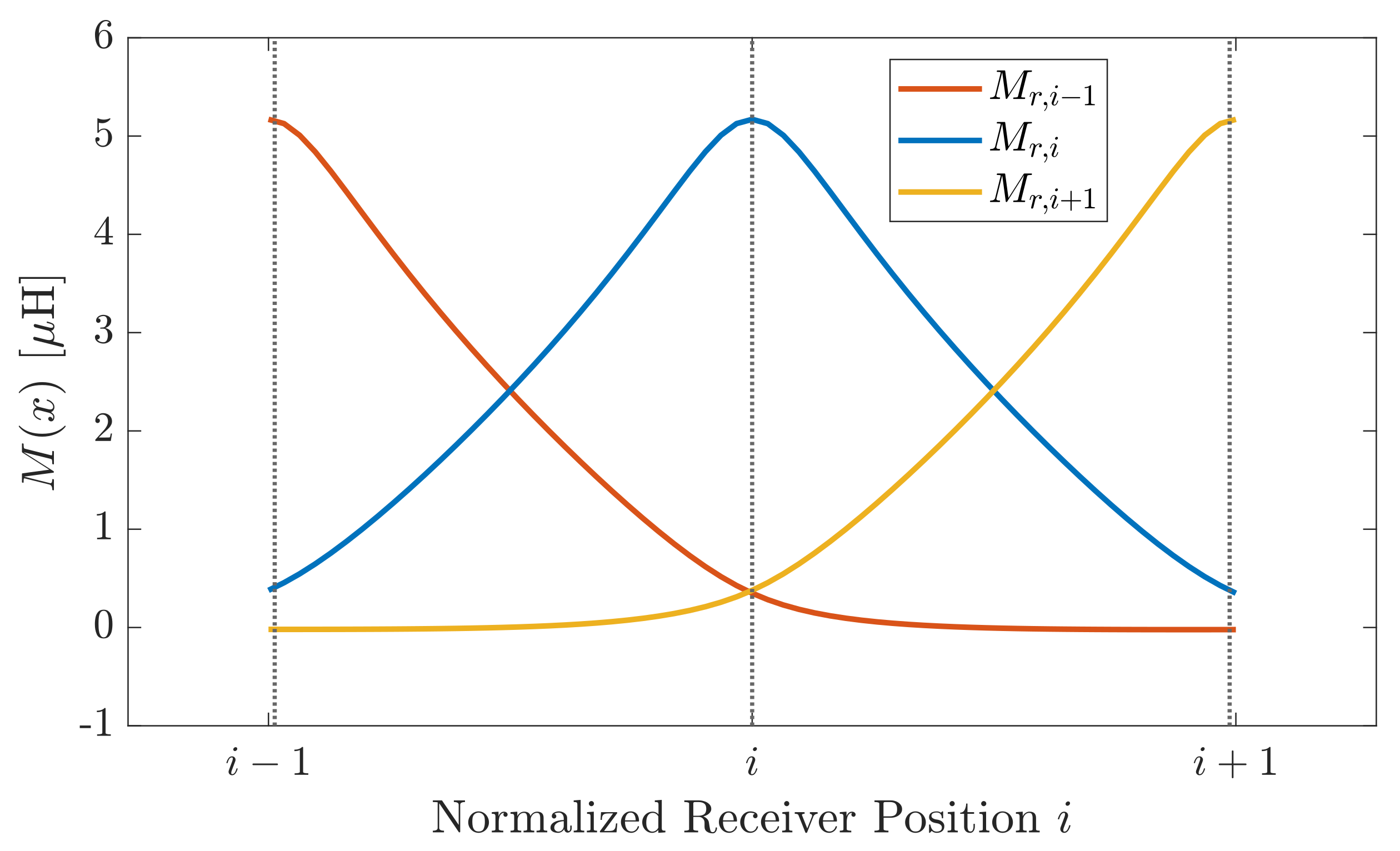
5. Resonator Array with a Receiver

Until now, resonator arrays have been considered to enhance the power transmission to the terminal resonator, which acts as a receiver for the WPT system. However, in the literature, a slightly different application is usually considered, that exploits the whole array as a transmitter, over which the receiver is free to move. This configuration increases the tolerance to the misalignment of the receiver circuit and represents a suitable solution for industry applications, e.g., for automation and EV charging. Furthermore, if the receiver moves over the resonators, it could offer the possibility of a dynamic power transfer. In this section, the configuration of a resonator array with a receiver shown in Figure 6 is analysed, making use of the approaches presented in Section 2 and highlighting its equivalent TL. Basically, the array is the same presented in Section 3, with a further resonator labelled r acting as a receiver, which for simplicity is identical to the array resonators and is placed 10 mm above the array. The load is connected to that resonator and ${\widehat{Z}}_{load}$ is its impedance, as represented in Figure 7. The last cell of the array is terminated in an additional impedance that can assume arbitrary values. There is now another parameter that affects the operation of the WPT system, which is the mutual inductance $M_{r,i}$ between the receiver circuit and the i-th resonator of the array facing the receiver. It depends on the geometry of the cells and the position x of the receiver along the array, which is described by the coordinate system represented in Figure 6. As all the resonators are identical, the mutual inductance, function of the position x, behaves as reported in Figure 8 for the receiver and three different consecutive resonators.

For a complete analysis, different positions of the receiver have been considered. As a consequence, the current of each resonator becomes a function of the receiver position.

5.1. Circuit Analysis

The circuit analysis is carried out as described in Section 2, with an additional KVL equation written for the receiver. The impedance matrix ${\widehat{\mathbf{Z}}}_{\mathbf{m}}$ now includes also the terms representing the coupling of the receiver with the array cells, which are different for each position of the receiver along the array. In general, in case the receiver is coupled with the ith and $(i+1)$th cells of the array, the impedance matrix is:

$${\widehat{\mathbf{Z}}}_{\mathbf{m}}=\left[\begin{array}{ccccccccccc}{\widehat{Z}}_S+\widehat{Z}& j\omega M& 0& 0& \cdots & \cdots & \cdots & \cdots & \cdots & \cdots & 0\\ j\omega M& \widehat{Z}& j\omega M& 0& \cdots & \cdots & \cdots & \cdots & \cdots & \cdots & 0\\ 0& \ddots & \ddots & \ddots & \cdots & \cdots & \cdots & \cdots & ⋮& ⋮& ⋮\\ ⋮& ⋮& \ddots & \ddots & \cdots & \cdots & \cdots & \cdots & ⋮& ⋮& ⋮\\ ⋮& ⋮& ⋮& \ddots & \cdots & \cdots & \cdots & \cdots & ⋮& ⋮& 0\\ ⋮& ⋮& ⋮& ⋮& \cdots & \cdots & \cdots & \cdots & ⋮& ⋮& j\omega M_{r,i}\\ ⋮& ⋮& ⋮& ⋮& \cdots & \cdots & \cdots & \cdots & ⋮& ⋮& j\omega M_{r,i+1}\\ ⋮& ⋮& ⋮& ⋮& \cdots & \cdots & \cdots & \cdots & ⋮& ⋮& 0\\ ⋮& ⋮& ⋮& ⋮& \cdots & \cdots & \cdots & \cdots & \ddots & \ddots & ⋮\\ 0& \cdots & \cdots & \cdots & \cdots & \cdots & \cdots & \cdots & j\omega M& \widehat{Z}+{\widehat{Z}}_T& 0\\ 0& \cdots & \cdots & \cdots & \cdots & j\omega M_{r,i}& j\omega M_{r,i+1}& \cdots & \cdots & 0& \widehat{Zr}\end{array}\right]$$

(20)

where the last row considers the coupling of the receiver with the ith and $(i+1)$th cells of the array for a receiver generic position, $\widehat{Z}=R+j\omega L+1/\left(j\omega C\right)$ is the impedance of the single cell and ${\widehat{Z}}_r=\widehat{Z}+{\widehat{Z}}_{load}$ is the impedance of the receiver.

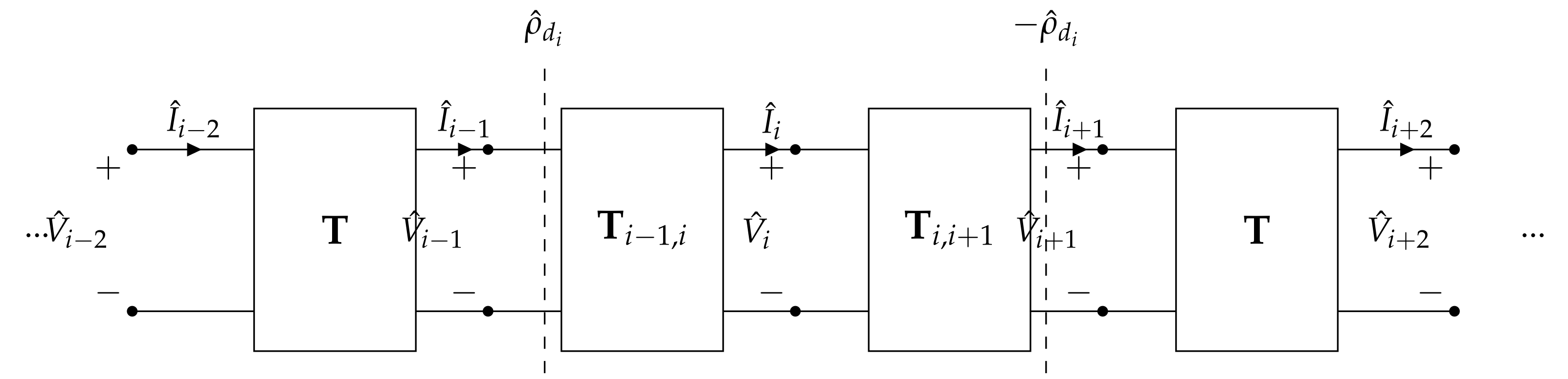
5.2. Equivalent Transmission Line

The structure of the apparatus can be studied with its equivalent TL, that allows interesting insights to be attained. Among the different models that can be proposed the most comprehensive one can be obtained considering the receiver as a further TL connected to the array, having the same length $\lambda /4$ of the resonators that form the array. However, as regards the array current analysis it is possible to simplify the equivalent TL as shown in the following for a receiver that couples to one or two array resonators.

5.2.1. Perfectly Aligned Receiver

In case the receiver couples to one resonator only, it is possible to simplify the system by embedding the reflected impedance ${\widehat{Z}}_d$ of the receiver into the equivalent circuit of the facing array resonator. In fact, according to [15,16,26], for a receiver coupled with the ith array cell, it is possible to write the KVL equation:

$$j\omega M{\widehat{I}}_{i-1}+(\widehat{Z}+{\widehat{Z}}_d){\widehat{I}}_i+j\omega M{\widehat{I}}_{i+1}=0$$

(21)

where

$${\widehat{Z}}_{d_i}=\frac{{\left(\omega M_{r,i}\left(x\right){|}_{\max }\right)}^2}{{\widehat{Z}}_r}.$$

(22)

The equivalent TL representing this system configuration can be obtained from that of the resonator array without a receiver considering the increased impedance $\widehat{Z}+{\widehat{Z}}_{d_i}$ of the ith resonator. The transmission matrices ${\mathbf{T}}_{i-1,i}$ and ${\mathbf{T}}_{i,i+1}$ representing the coupling between the ith resonator and the adjacent ones ($i-1$ and $i+1$, respectively) modify consequently, as ${\widehat{Z}}_i$ in (4) becomes ${\widehat{Z}}_i=(\widehat{Z}+{\widehat{Z}}_{d_i})/2$, while the mutual impedance ${\widehat{Z}}_{M_{i,i+1}}$ is not altered. By using (10), the segment of MI waveguide composed of the two-port networks represented by the modified transmission matrices ${\mathbf{T}}_{i-1,i}$ and ${\mathbf{T}}_{i,i+1}$ presents a characteristic impedance ${\widehat{Z}}_{0_{i-1,i}}={\widehat{Z}}_{0_{i,i+1}}={\widehat{Z}}_{0_d}\ne {\widehat{Z}}_0$. Thus, at the interfaces between TL segments of different characteristic impedances, shown in Figure 9 by vertical dashed lines, there occur reflections of MI waves that come from the power source and the termination. The reflection phenomenon can be understood by means of the reflection coefficient at the interfaces. For forward MI waves travelling from the power source towards the termination (positive x direction), the reflection coefficient at the interface between the $i-1$ and i cells is

$${\widehat{\rho }}_{d_i}=\frac{{\widehat{Z}}_{0_d}-{\widehat{Z}}_0}{{\widehat{Z}}_{0_d}+{\widehat{Z}}_0},$$

(23)

and $-{\widehat{\rho }}_{d_i}$ at the interface between the i and $i+1$ cells, whereas the opposite should be considered for backward MI waves travelling in the negative x direction. According to [16], the exact receiver matching is achieved in resonance when ${\widehat{Z}}_{load}={\widehat{Z}}_{load}^m$ where

$${\widehat{Z}}_{load}^m=\frac{{\omega }_0{M}_{r,i}^2\left(x\right){|}_{\max }}{M{e}^{-\alpha d}}-R,$$

(24)

a condition very difficult to meet, since the receiver load is defined by the circuitry connected to it.

5.2.2. Receiver Coupled with Two Array Resonators

In case the receiver is coupled with the ith and $(i+1)$th resonators, a reflected impedance and a controlled voltage source have to be added in the ith and $(i+1)$th cells. Thus, the impedances of the ith and $(i+1)$th resonators and the mutual impedances between the ith and $(i+1)$th resonators and the adjacent ones modify accordingly, altering the parameters of the transmission matrices ${\mathbf{T}}_{i-1,i}$, ${\mathbf{T}}_{i,i+1}$ and ${\mathbf{T}}_{i+1,i+2}$. The resulting equivalent TL is depicted in Figure 10. The values of the modified matrix elements can be derived considering the KVL equations written for the receiver and the ith and $(i+1)$th array resonators:

$$j\omega M_{r,i}{\widehat{I}}_i+j\omega M_{r,i+1}{\widehat{I}}_{i+1}+{\widehat{Z}}_r{\widehat{I}}_r=0$$

(25)

$$j\omega M{\widehat{I}}_{i-1}+\widehat{Z}{\widehat{I}}_i+j\omega M{\widehat{I}}_{i+1}+j\omega M_{r,i}{\widehat{I}}_r=0$$

(26)

$$j\omega M{\widehat{I}}_i+\widehat{Z}{\widehat{I}}_{i+1}+j\omega M{\widehat{I}}_{i+2}+j\omega M_{r,i+1}{\widehat{I}}_r=0$$

(27)

Substituting ${\widehat{I}}_r$ from (25) in (26) and (27) we obtain:

$$j\omega M{\widehat{I}}_{i-1}+\left(\widehat{Z}+{\widehat{Z}}_{d_i}\left(x\right)\right){\widehat{I}}_i+\left(j\omega M+{\widehat{Z}}_{d_{i,i+1}}\left(x\right)\right){\widehat{I}}_{i+1}=0$$

(28)

and

$$\left(j\omega M+{\widehat{Z}}_{d_{i,i+1}}\left(x\right)\right){\widehat{I}}_i+\left(\widehat{Z}+{\widehat{Z}}_{d_{i+1}}\left(x\right)\right){\widehat{I}}_{i+1}+j\omega M{\widehat{I}}_{i+2}=0$$

(29)

where

$${\widehat{Z}}_{d_i}\left(x\right)={\omega }^2\frac{M_{r,i}{\left(x\right)}^2}{{\widehat{Z}}_r}$$

(30)

$${\widehat{Z}}_{d_{i+1}}\left(x\right)={\omega }^2\frac{M_{r,i+1}{\left(x\right)}^2}{{\widehat{Z}}_r}$$

(31)

$${\widehat{Z}}_{d_{i,i+1}}\left(x\right)={\omega }^2\frac{M_{r,i}\left(x\right)M_{r,i+1}\left(x\right)}{{\widehat{Z}}_r}$$

(32)

The new terms of ${\mathbf{T}}_{i-1,i}$, ${\mathbf{T}}_{i,i+1}$ and ${\mathbf{T}}_{i+1,i+2}$ can be found according to (4) considering:

$$\begin{array}{cc}\hfill {\widehat{Z}}_i\left(x\right)& =\frac{\widehat{Z}+{\widehat{Z}}_{d_i}\left(x\right)}{2}\hfill \end{array}$$

(33)

$$\begin{array}{cc}\hfill {\widehat{Z}}_{i+1}\left(x\right)& =\frac{\widehat{Z}+{\widehat{Z}}_{d_{i+1}}\left(x\right)}{2}\hfill \end{array}$$

(34)

and

$${\widehat{Z}}_{M_{i,i+1}}\left(x\right)={\widehat{Z}}_{M_{i+1,1}}\left(x\right)=j\omega M+{\widehat{Z}}_{d_{i,i+1}}\left(x\right),$$

(35)

whereas the characteristic impedances of the TL segments are found with (10). It must be noticed that, as the mutual impedance is not purely imaginary, the resulting characteristic impedances are not real anymore. Moreover, they are different for each line segment, which considers resonators coupled with the receiver and depend on the receiver position x, with consequent MI wave reflections due to the impedance discontinuities. In general, ${\widehat{Z}}_{0_{i-1,i}}\left(x\right)\ne {\widehat{Z}}_{0_{i,i+1}}\left(x\right)\ne {\widehat{Z}}_{0_{i+1,i+2}}\left(x\right)\ne {\widehat{Z}}_0$. The reflection coefficients at the interfaces, that are different and complex, can be generally defined, for forward MI waves, as:

$${\widehat{\rho }}_{i,i+1}\left(x\right)=\frac{{\widehat{Z}}_{0_{i,i+1}}\left(x\right)-{\widehat{Z}}_{0_{i-1,i}}\left(x\right)}{{\widehat{Z}}_{0_{i,i+1}}\left(x\right)+{\widehat{Z}}_{0_{i-1,i}}\left(x\right)}$$

(36)

and are schematically shown in Figure 10. The opposite value should be considered for backward MI waves. The equivalent TL can be considered as the union of three TL segments: the first comprising the resonators from the 1th to the $(i-1)$th, the second composed of the resonators coupled to the receiver (two-port networks represented by ${\mathbf{T}}_{i-1,i}$, ${\mathbf{T}}_{i,i+1}$ and ${\mathbf{T}}_{i+1,i+2}$) and the third comprising the resonators from the $(i+2)$th to the last one. In particular, the first and third segments of the TL result to be longer or shorter depending on the receiver position.

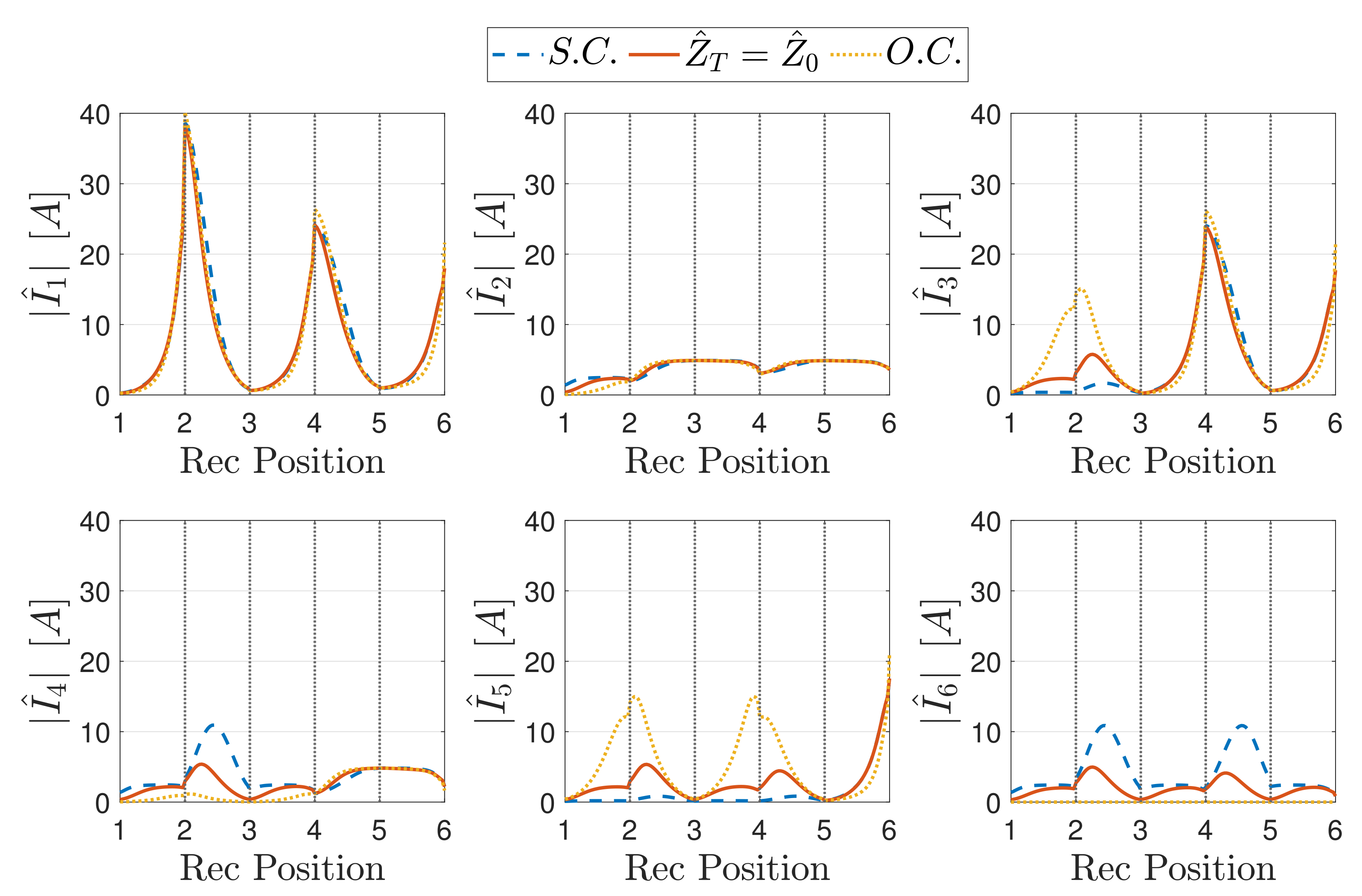
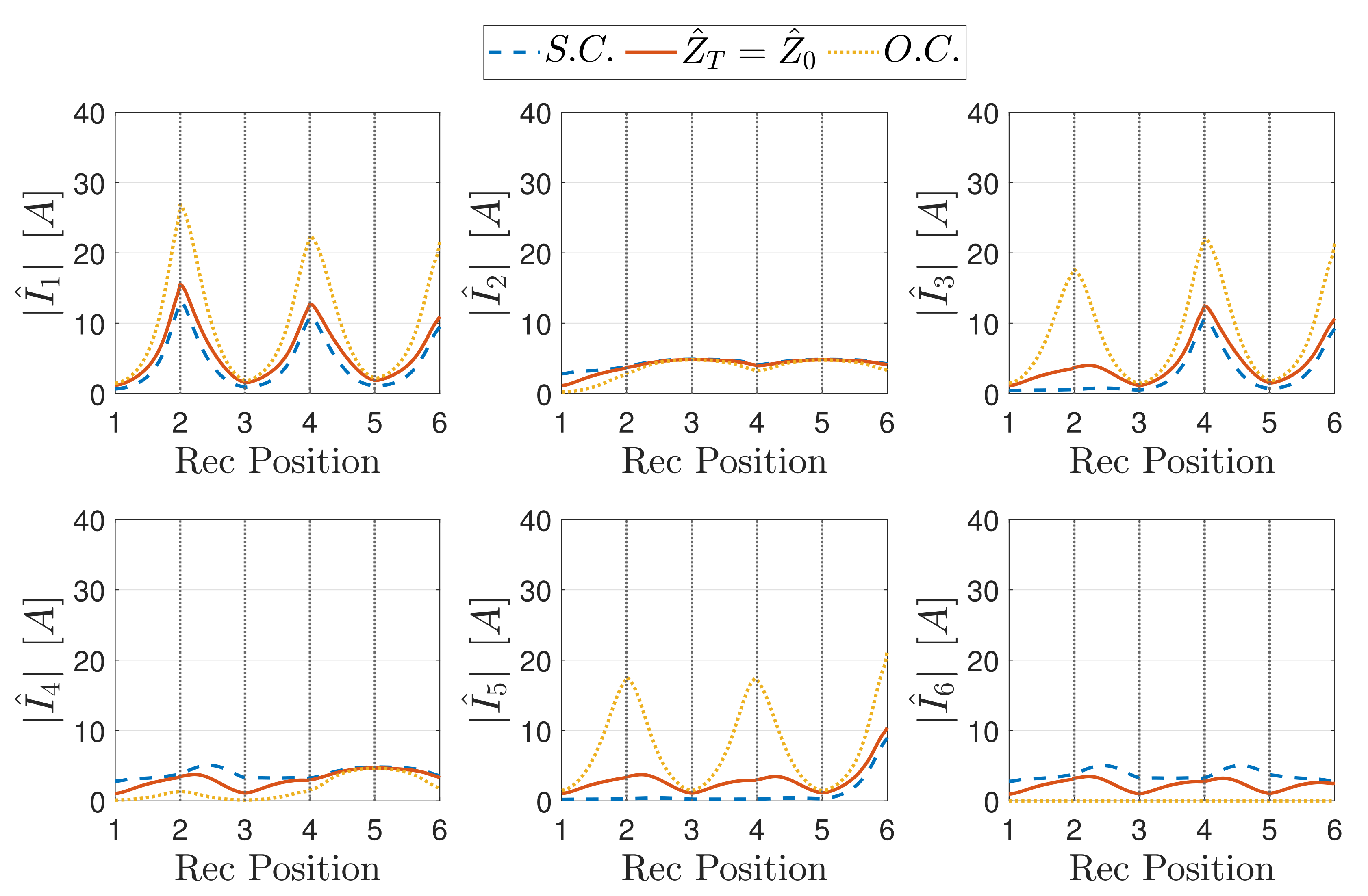
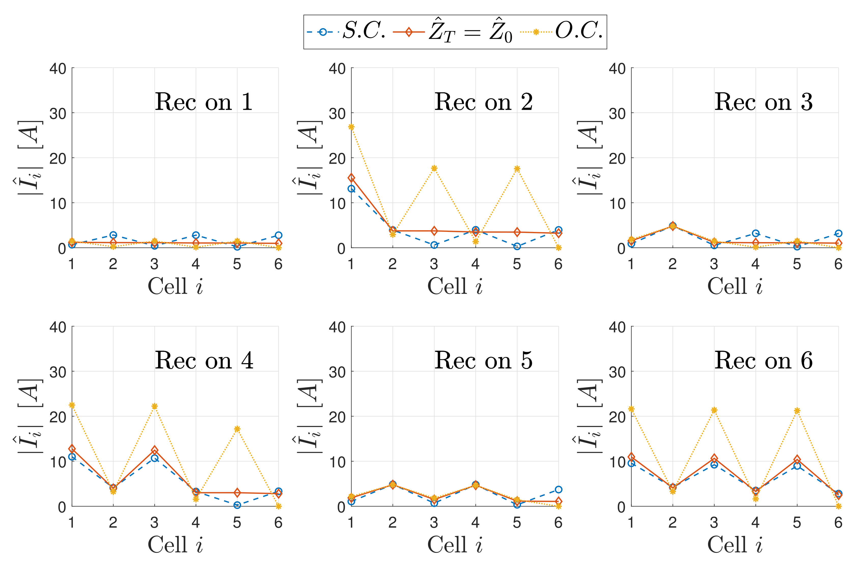
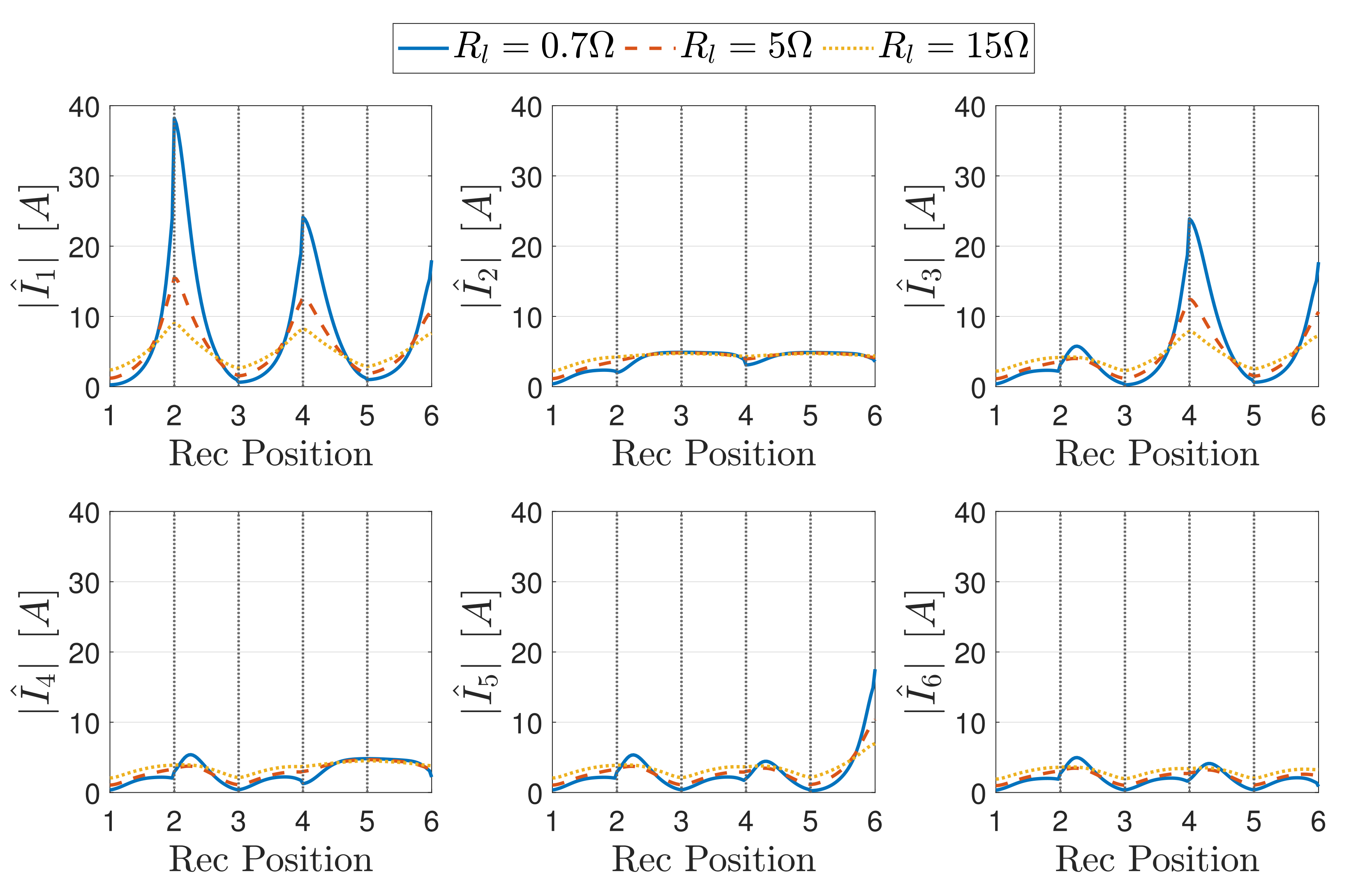
5.3. Numerical Simulations

In this section, the results of numerical simulations of the array prototype used for the experiments (and described in Section 6) are presented and discussed. The characteristic impedance of the array is ${\widehat{Z}}_0\approx 1.5$$\Omega$ and different simulations have been performed considering matched and modulated terminations and load impedance values of $0.7$$\Omega$, 5 $\Omega$ and 15 $\Omega$. To simulate the continuous variation of the receiver position, a small discretisation step $\Delta x=d/30$ has been set.

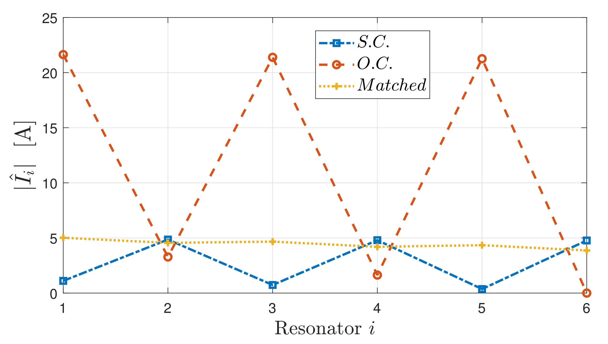
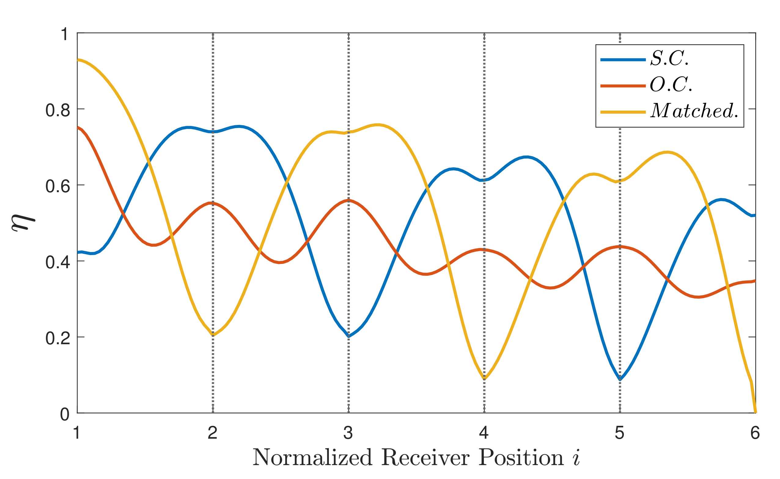
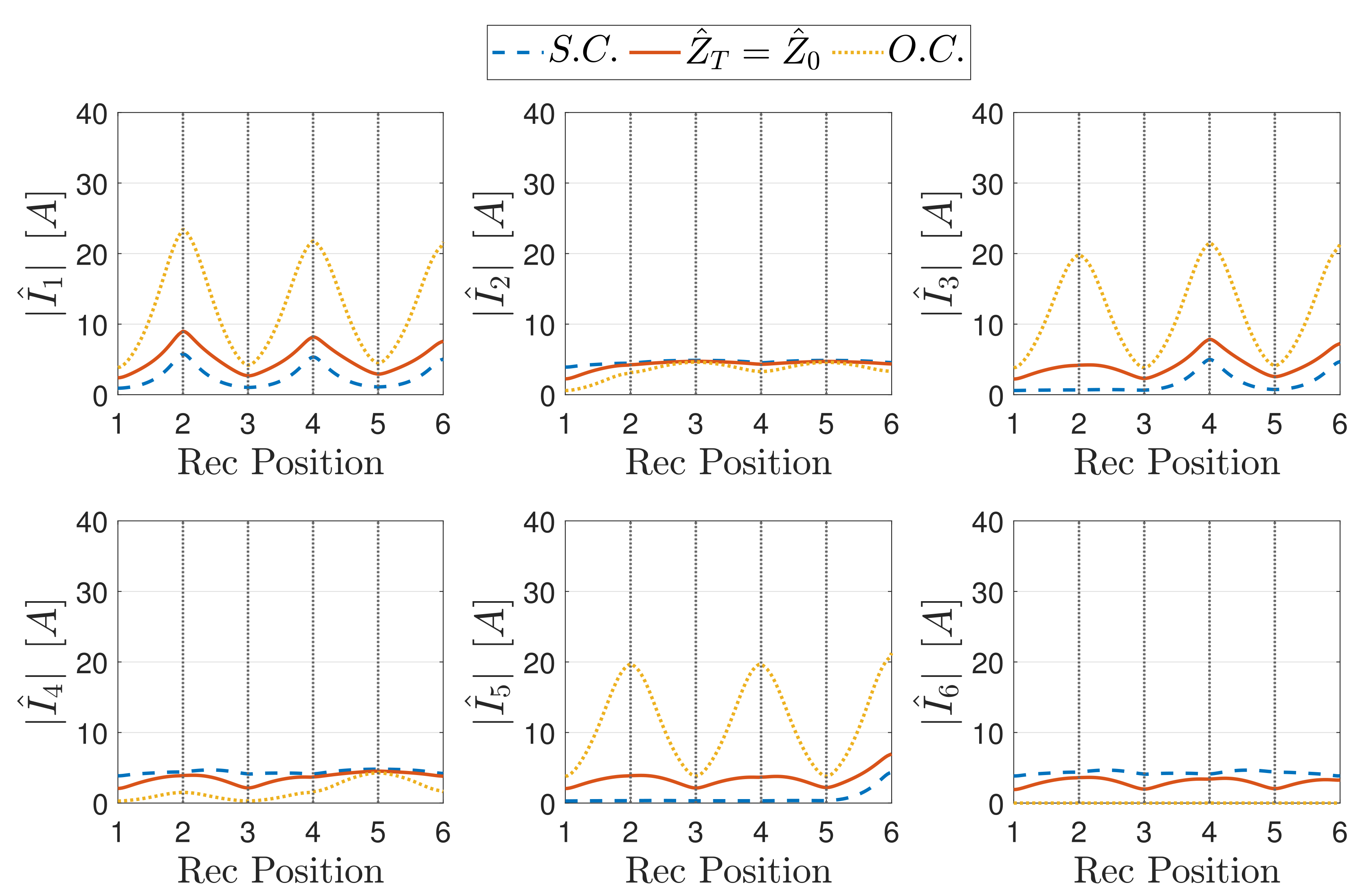
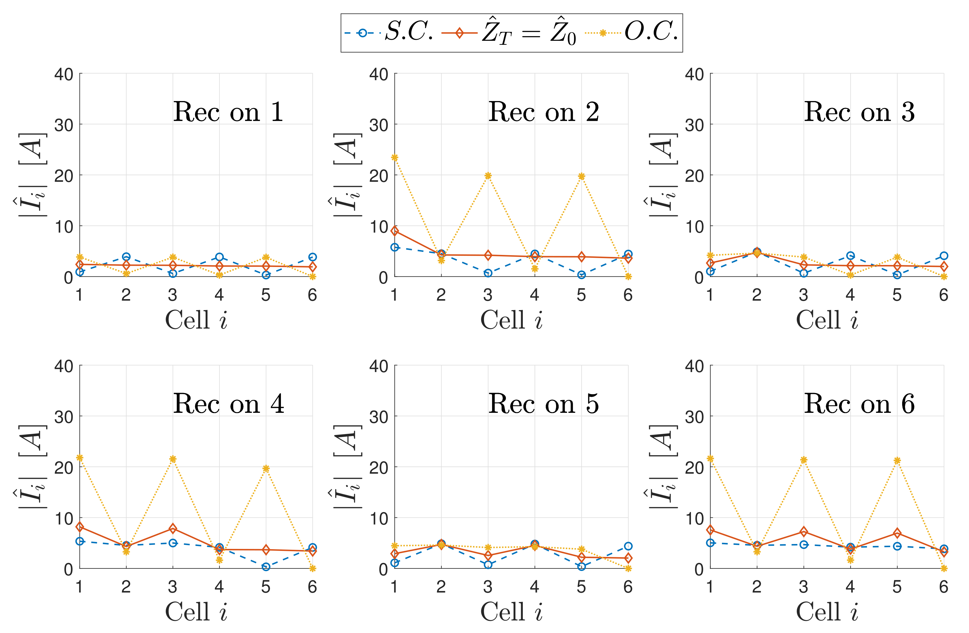
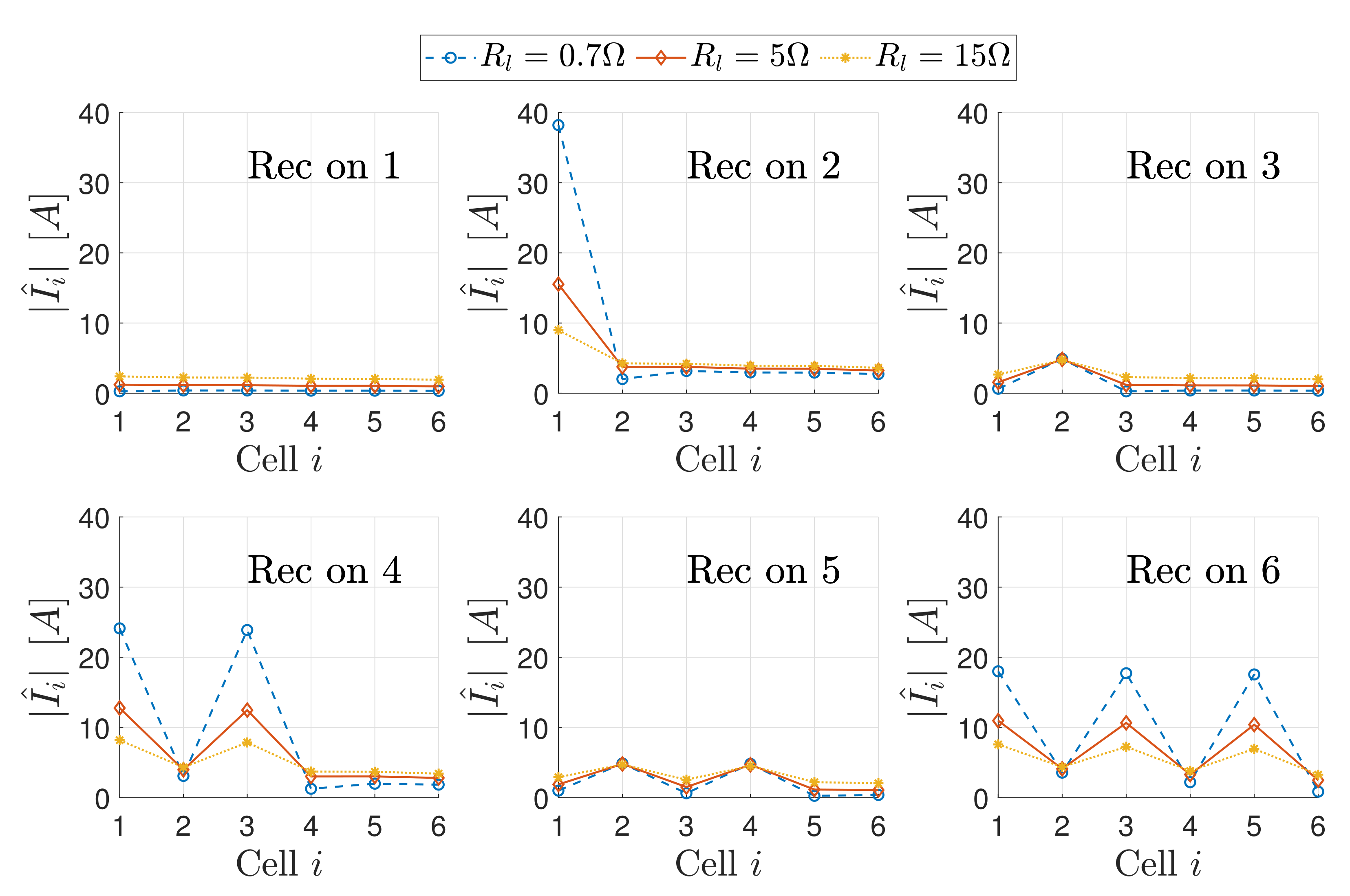
5.3.1. Currents for a Matched Array

The termination impedance of the array ${\widehat{Z}}_T$, which can be considered the unique degree of freedom during the operation, can seriously affect the performance of the apparatus. In particular, as a first choice, it seems convenient to set ${\widehat{Z}}_T={\widehat{Z}}_0$, i.e., matching only the array. In this way, the amount of power that is transferred in the TL segment after the discontinuity introduced by the receiver does not undergo reflections and is completely absorbed by the termination impedance.

In Figure 11 the current magnitudes of the resonators are reported as a function of the receiver position for different values of the load resistance. The plots suggest the presence of standing wave patterns for the MI waves and indicate that the most severe current peaks occur when the receiver is perfectly aligned with a resonator. For a better visualization of the standing wave patterns, the resonator current magnitudes are plotted for different values of the load resistance in Figure 12, considering only the position of perfect alignment since it leads to the highest current magnitudes. As it can be expected, no standing waves occur for the segment of the TL after the resonator covered by the receiver, with the overt case when the receiver is placed over the first resonator of the array. The reflections caused by the impedance discontinuity are more evident when the receiver is close to the power source, since this situation corresponds to the shortest equivalent TL, confirming what discussed in Section 4.1 and observed in Figure 5.

The presence of the termination impedance allows the TL segment to be matched at the cost of decreasing the efficiency, since it dissipates the incident power. In order to increase the efficiency, it is convenient to keep the traveling power inside the waveguide and this can be achieved with both S.C. and O.C. terminations. The resulting transmission efficiency is reported for a generic receiver position in Figure 13 in the case of a load resistance of 5 $\Omega$. The curves mirror the efficiency trend in the case of O.C. and S.C. terminations, whereas a strong efficiency reduction occurs in the case of a matched array.

5.3.2. Modulated Termination

The standing wave patterns of the efficiency, shown in Figure 13, suggest the possibility of adjusting the termination impedance of the array so that an efficiency peak is obtained at the position of the receiver. Among the proposed modulation techniques [27,28], the simplest idea consists in changing the termination condition from S.C. to O.C., leading to a shift in the standing wave pattern of the current with a consequent shift in the position of the efficiency peaks.

In this way, the power-transfer efficiency is nearly constant for each position of the receiver along the array, even if current peaks can occur in the resonators upstream and downstream the ones facing the receiver. In general, the MI wave transmitted downstream of the receiver undergoes reflection at the termination and, in turn, also at the discontinuity created by the receiver, causing standing wave patterns in each section of the equivalent TL.

The magnitude of the resonator currents as a function of the receiver position and the relevant standing wave patterns for a perfectly aligned receiver are plotted in Figure 14, Figure 15, Figure 16, Figure 17, Figure 18 and Figure 19 in the case of S.C., O.C. and perfectly matched termination for different receiver load values. In particular, Figure 14 and Figure 15 refer to ${\widehat{Z}}_{load}=0.7$$\Omega$, Figure 16 and Figure 17 to ${\widehat{Z}}_{load}=5$$\Omega$ and Figure 18 and Figure 19 to ${\widehat{Z}}_{load}=15$$\Omega$.

These values have been chosen to cover all the possible load conditions that can occur. Indeed, the matching load of the receiver circuit ${\omega }_0{M}_{r,i}\left(x\right)$ is 5 $\Omega$ in the case of perfect alignment conditions. Then, the values $0.7$$\Omega$ and 15 $\Omega$ have been considered to simulate low- and high-impedance conditions, respectively. Moreover, the load ${\widehat{Z}}_{load}=15$$\Omega$ theoretically guarantees the matching of the receiver to the array and is calculated by (24).

The plots highlight that the resonators covered by the receiver experience low current values, whereas the most severe peaks occur when the receiver covers the even resonators. Analysing the worst scenarios, it is possible to state that the receiver load ${\widehat{Z}}_{load}$ affects the amplitude of the current peaks, whereas their position is determined by the length and the boundary conditions of the equivalent TL (input and termination impedances). Considering typical loads connected to the receiver, i.e., battery charging systems, the reflected impedance from the receiver ${\widehat{Z}}_{d_i}$ is real and then the phase shift experienced by the MI waves along the line is not altered, despite further reflections occur. The resulting standing wave pattern can be explained considering the defect impedance introduced by the receiver and the lengths of the TL segments upstream and downstream of the discontinuity.

Case ${\widehat{Z}}_{load}=0.7$ $\Omega$

For low values of ${\widehat{Z}}_{load}$ ($|{\widehat{Z}}_{load}|<|{\widehat{Z}}_{load}^m\left)\right|$), the receiver reflected impedance presents very high values and the array resonator covered by the receiver behaves as an open circuit, as (30), (31) and (32) show. In the case of perfect alignment, the upstream TL segment is formed by $i-1$ resonators and terminates in S.C., while the downstream one is composed of $n-i$ cells and is terminated in ${\widehat{Z}}_T$. Thus, according to Section 4.1 (see Figure 5), the upstream SWR has higher values if i is even, while the downstream segment experiences higher SWR values if $n-i$ is odd with ${\widehat{Z}}_T=0$ or $n-i$ is even with ${\widehat{Z}}_T\to \infty$, as it is possible to see from Figure 15. In the case the receiver couples to two resonators i and $i+1$, the same considerations hold, where the upstream TL segment composed of $i-1$ cells and the downstream one of $n-(i+1)$ cells. Overall, the current behaviour in the two line segments varies according to the receiver position, which determines their effective lengths and terminations, as it is shown in Figure 14. It should be observed that, if the receiver covers an odd cell, the standing wave pattern occurred in the upstream TL segment makes the magnitude of the first resonator current very low compared to the previous situation, thereby reducing the power demand to the supply system.

An exception is observed in the array current distribution of the downstream TL segment for S.C. and matched termination. In these conditions, the even cells experience current peaks when the receiver is placed between an even and an odd cell. This may be explained considering that both upstream and downstream TL segments are composed of an odd number of cells and thus their SWRs have higher values, as discussed in Section 4.1.

Case ${\widehat{Z}}_{load}=5$ $\Omega$

If the receiver load increases, its reflected impedance decreases as (30) shows, and the resulting equivalent TL is getting closer to the case of the array without receiver, for which the standing wave pattern is shown in Figure 4. As Figure 16 and Figure 17 show, the trends of the currents and the SWRs are similar to those of the previous case. It can be noticed that the current values are smaller, which is the discontinuity introduced by the receiver smaller.

Case ${\widehat{Z}}_{load}=15$ $\Omega$

Finally, Figure 18 and Figure 19 show that for a value of ${\widehat{Z}}_{load}=15$$\Omega$, which guarantees the matching for perfect alignment positions and is obtained from (24), the upstream equivalent TL segment is matched when the impedance ${\widehat{Z}}_i$ of the resonator facing the receiver is ${\widehat{Z}}_0$ (${\widehat{\rho }}_{d_i}=0$). In general, ${\widehat{Z}}_i=\widehat{Z}+{\widehat{Z}}_{d_i}+{\widehat{Z}}_{TL,down}$, where ${\widehat{Z}}_{TL,down}$ is the reflected impedance of the downstream TL segment to the ith resonator, whose value varies between zero and infinity depending on its length and termination, as shown in [26]. For a low-loss array ${\widehat{Z}}_i\approx {\widehat{Z}}_{d_i}+{\widehat{Z}}_{TL,down}$ and thus, considering the receiver matched, ${\widehat{Z}}_i\approx {\widehat{Z}}_0$ only if ${\widehat{Z}}_{TL,down}\approx 0$, namely only if:

• The downstream TL segment is composed of an even number of resonators and is terminated in S.C.;
• The downstream TL segment is composed of an odd number of resonators and is terminated in O.C.

This can be appreciated from Figure 19, which illustrates the standing wave patterns. When the upstream TL segment is matched, the upstream resonator currents are all equal. However, for generic receiver positions standing waves still occur and the highest currents magnitudes are found for an array with an odd number of resonators, as Figure 18 shows.

Overall, the presented results clearly indicate that, although a proper modulation of the termination of the array allows the efficiency to be dramatically improved, for generic receiver positions the resonators can experience very large currents, which may potentially lead to a breakdown of the whole apparatus.

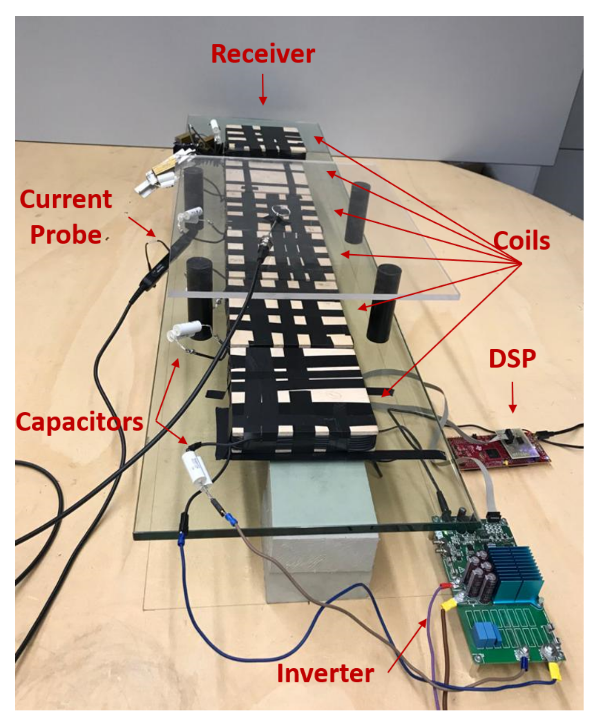
6. Experimental Verification

The numerical results have been experimentally verified considering the array represented in Figure 6, in the case of perfect matching of the termination and a load of 5 $\Omega$. In Figure 6 all the components of the experimental system are indicated. The array prototype, shown in Figure 20, is composed of six stranded-wire resonators (coils), each made with six square turns of 153 mm side-length. The winding conductors have a section of 2.5 mm${}^2$, resulting in an intrinsic resistance $R=0.11$$\Omega$ and a self-inductance $L=12.5$$\mathsf{\mu }$H. The terminals of each resonator are connected to a capacitor of capacitance $C=93.1$ nF, so that the coils resonate at a frequency $f_0=147$ kHz. This array is characterized by a mutual inductance $M=-1.55$$\mathsf{\mu }$H between adjacent resonators, resulting in a characteristic impedance ${\widehat{Z}}_0\simeq 1.5$$\Omega$. The input voltage downstream of the supply system is set to $3.6V_{rms}$ and is provided by a half-bridge inverter realized with GaN transistors, with an internal impedance ${\widehat{Z}}_S=0.01$$\Omega$. The currents have been measured by means of a current probe Tektronix TCP302 amplified by a Tektronix “TCPA 300” and processed through an Agilent “Infiniium” 54855A oscilloscope with a sampling capability of 2 GSa/s and a bandwidth of 500 MHz. The measurements refer to the current magnitude of each resonator versus the position of the receiver along the array, considering the array terminated in a resistance of 1.5 $\Omega$ and the receiver connected to a 5 $\Omega$ resistive load. The results of the measurements are reported in Figure 21 and are compared with the numerical predictions (see Figure 11 and Figure 16). As expected, the measurement reveals the presence of standing wave patters for the MI wave (current wave), with the highest magnitude values in correspondence to the positions of perfect alignment of the receiver with even resonators. The comparison between measurements and numerical simulations shows a very good agreement; the maximum difference between the trends is found in correspondence of the current peak values, with an error of about 3.5%.

7. Conclusions

Inductive power transfer systems employing an array of magnetically coupled resonators allow the power transfer range to be extended, preserving a great efficiency. In this paper the resonator arrays are studied exploiting the analogy with the TLs, which is possible describing the array as a cascade of transmission matrices. This approach has been discussed for generic arrays and permits the system behaviour to be analytically investigated, as well as it provides insights about the phenomena that occur. In the first part of the work arrays with a load impedance connected to the last resonator are considered. An analytical expression for the resonator currents of a generic array has been proposed and validated, in the hypothesis of “nearest-neighbourhood interaction”. Both analytical and numerical studies highlight strong current peaks occurring for particular configurations reported and discussed in Section 4. The analysis of resonator arrays fed by an inverter has shown critical standing wave ratios in case the arrays is composed of an odd number of resonators. The second part of the work is devoted to the analysis of resonator arrays with a receiver and shows how the TL model can be extended to these apparatuses. The definition of the transmission matrices has been extended to case of a receiver in a generic position, allowing an estimation of the current behaviour in the array. Different modulation strategies have been presented in order to reach a uniform efficiency for all the receiver positions along the array, at the expense of standing wave patterns of the resonator currents. The presence of a receiver leads to discontinuities in the array causing reflections and then high current peaks, which in turn may lead to severe stress to the electric components. This clearly indicates that the resonators have to be properly tailored, still preserving the same impedance as well as the same mutual inductance, in order to avoid further impedance discontinuities. With a proper design, resonator arrays can be considered a very cheap solution to extend WPT.

References

1. Bi, S.; Ho, C.K.; Zhang, R. Wireless powered communication: Opportunities and challenges. IEEE Commun. Mag. 2015, 53, 117–125. [Google Scholar] [CrossRef] [Green Version]
2. Covic, G.A.; Boys, J.T. Modern trends in inductive power transfer for transportation applications. IEEE J. Emerg. Sel. Top. Power Electron. 2013, 1, 28–41. [Google Scholar] [CrossRef]
3. Covic, G.A.; Boys, J.T. Inductive power transfer. Proc. IEEE 2013, 101, 1276–1289. [Google Scholar] [CrossRef]
4. Patil, D.; McDonough, M.K.; Miller, J.M.; Fahimi, B.; Balsara, P.T. Wireless Power Transfer for Vehicular Applications: Overview and Challenges. IEEE Trans. Transp. Electrif. 2017, 4, 3–37. [Google Scholar] [CrossRef]
5. Hassan, N.U.; Lee, W.; Lee, B. Efficient, Load Independent and Self-Regulated Wireless Power Transfer with Multiple Loads for Long Distance IoT Applications. Energies 2021, 14, 1035. [Google Scholar] [CrossRef]
6. Schuylenbergh, K.V.; Puers, R. Inductive Powering: Basic Theory and Application to Biomedical Systems, 1st ed.; Springer Science: Dordrecht, The Netherlands, 2009. [Google Scholar]
7. RamRakhyani, A.K.; Mirabbasi, S.; Chiao, M. Design and optimization of resonance-based efficient wireless power delivery systems for biomedical implants. IEEE Trans. Biomed. Circuits Syst. 2011, 5, 48–63. [Google Scholar] [CrossRef] [PubMed]
8. Moon, S.; Kim, B.C.; Cho, S.Y.; Ahn, C.H.; Moon, G.W. Analysis and design of a wireless power transfer system with an intermediate coil for high efficiency. IEEE Trans. Ind. Electron. 2014, 61, 5861–5870. [Google Scholar] [CrossRef]
9. Moon, S.C.; Moon, G.W. Wireless Power Transfer System with an Asymmetric Four-Coil Resonator for Electric Vehicle Battery Chargers. IEEE Trans. Power Electron. 2016, 31, 6844–6854. [Google Scholar] [CrossRef]
10. Yu, H.; Zhang, G.; Jing, L.; Liu, Q.; Yuan, W.; Liu, Z.; Feng, X. Wireless power transfer with HTS transmitting and relaying coils. IEEE Trans. Appl. Supercond. 2015, 25. [Google Scholar] [CrossRef]
11. Hui, S.Y.R.; Zhong, W.; Lee, C.K. A Critical Review of Recent Progress in Mid-Range Wireless Power Transfer. IEEE Trans. Power Electron. 2014, 29, 4500–4511. [Google Scholar] [CrossRef] [Green Version]
12. Zhong, W.; Lee, C.K.; Hui, S.Y.R. General Analysis on the Use of Tesla’s Resonators in Domino Forms for Wireless Power Transfer. IEEE Trans. Ind. Electron. 2013, 60, 261–270. [Google Scholar] [CrossRef] [Green Version]
13. Stevens, C.J. Some consequences of the properties of metamaterials for wireless power transfer. In Proceedings of the 2015 9th International Congress on Advanced Electromagnetic Materials in Microwaves and Optics, METAMATERIALS 2015, Oxford, UK, 7–12 September 2015; pp. 295–297. [Google Scholar] [CrossRef]
14. Simonazzi, M.; Sandrolini, L.; Zarri, L.; Reggiani, U.; Alberto, J. Model of Misalignment Tolerant Inductive Power Transfer System for EV Charging. In Proceedings of the IEEE International Symposium on Industrial Electronics, Delft, The Netherlands, 17–19 June 2020; pp. 1617–1622. [Google Scholar] [CrossRef]
15. Alberto, J.; Reggiani, U.; Sandrolini, L.; Albuquerque, H. Accurate calculation of the power transfer and efficiency in resonator arrays for inductive power transfer. Prog. Electromagn. Res. B 2019, 83, 61–76. [Google Scholar] [CrossRef] [Green Version]
16. Stevens, C.J. Magnetoinductive waves and wireless power transfer. IEEE Trans. Power Electron. 2015, 30, 6182–6190. [Google Scholar] [CrossRef]
17. Zhang, F.; Hackworth, S.A.; Fu, W.; Li, C.; Mao, Z.; Sun, M. Relay Effect of Wireless Power Transfer Using Strongly Coupled Magnetic Resonances. IEEE Trans. Magn. 2011, 47, 1478–1481. [Google Scholar] [CrossRef]
18. Kim, J.; Son, H.C.; Kim, K.H.; Park, Y.J. Efficiency Analysis of Magnetic Resonance Wireless Power Transfer With Intermediate Resonant Coil. IEEE Antennas Wirel. Propag. Lett. 2011, 10, 389–392. [Google Scholar] [CrossRef]
19. Shamonina, E.; Kalinin, V.A.; Ringhofer, K.H.; Solymar, L. Magnetoinductive waves in one, two, and three dimensions. J. Appl. Phys. 2002, 92, 6252–6261. [Google Scholar] [CrossRef]
20. Solymar, L.; Shamonina, E. Waves in Metamaterials; OUP Oxford: New York, NY, USA, 2009. [Google Scholar]
21. Worapishet, A. A Simplified Lossless Analysis of Magnetoinductive Waveguides for Investigation of Impedance Termination on Power Nulling Characteristics. Eng. Trans. 2021, 24, 170–175. [Google Scholar]
22. Syms, R.R.A.; Young, I.R.; Solymar, L. Low-loss magneto-inductive waveguides. J. Phys. D Appl. Phys. 2006, 39, 3945. [Google Scholar] [CrossRef]
23. Puccetti, G.; Stevens, C.J.; Reggiani, U.; Sandrolini, L. Experimental and numerical investigation of termination impedance effects in wireless power transfer via metamaterial. Energies 2015, 8, 1882. [Google Scholar] [CrossRef]
24. Joines, W.T.; Palmer, W.D.; Bernhard, J.T. Microwave Transmission Line Circuits, 1st ed.; Artech House: Norwood, MA, USA, 2012. [Google Scholar]
25. Chipman, R.A. Schaum’s Outline of Theory and Problems of Transmission Lines; McGraw-Hill: New York, NY, USA, 1968; p. 236. [Google Scholar]
26. Alberto, J.; Reggiani, U.; Sandrolini, L. Circuit model of a resonator array for a WPT system by means of a continued fraction. In Proceedings of the 2016 IEEE 2nd International Forum on Research and Technologies for Society and Industry Leveraging a Better Tomorrow, RTSI 2016, Bologna, Italy, 7–9 September 2016. [Google Scholar] [CrossRef]
27. Sandoval, F.S.; Moazenzadeh, A.; Delgado, S.M.T.; Wallrabe, U. Double-spiral coils and live impedance modulation for efficient wireless power transfer via magnetoinductive waves. In Proceedings of the 2016 IEEE Wireless Power Transfer Conference (WPTC), Aveiro, Portugal, 5–6 May 2016; pp. 1–4. [Google Scholar] [CrossRef]
28. Sandoval, F.S.; Moazenzadeh, A.; Wallrabe, U. Comprehensive Modeling of Magnetoinductive Wave Devices for Wireless Power Transfer. IEEE Trans. Power Electron. 2018, 33, 8905–8915. [Google Scholar] [CrossRef]
Figure 1. Array of R-L-C resonators as inductive coupling device of a battery charger.
Energies 15 00652 g001
Figure 2. Equivalent circuits of a resonator array (a) circuit fed by a half-bridge inverter and connected to a load and (b) approximate circuit for the first harmonic.
Energies 15 00652 g002
Figure 3. Equivalent representation of a resonator array by a cascade connection of two-port networks.
Energies 15 00652 g003
Figure 4. Current standing wave patterns for different termination loads.
Energies 15 00652 g004
Figure 5. Standing wave ratio for arrays of different length and different termination conditions.
Energies 15 00652 g005
Figure 6. Resonator array with a receiver.
Energies 15 00652 g006
Figure 7. Equivalent circuit of a resonator array with a receiver.
Energies 15 00652 g007
Figure 8. Mutual inductance between the receiver and three consecutive resonators of the array, as a function of the receiver position at a receiver height of 10 mm.
Energies 15 00652 g008
Figure 9. Section of the equivalent TL of a resonator array with a receiver coupled with the ith resonator.
Energies 15 00652 g009
Figure 10. Section of the equivalent TL of a resonator array with a receiver coupled with the ith and ( i + 1 ) th resonators.
Energies 15 00652 g010
Figure 11. Current magnitude of each resonator as a function of the receiver position, for a matched array and different load resistances.
Energies 15 00652 g011
Figure 12. Standing wave patterns for different positions of the perfectly aligned receiver, a matched array and different load resistances.
Energies 15 00652 g012
Figure 13. Transmission efficiency in the cases of S.C., O.C. and matched terminations for R l = 5 Ω .
Energies 15 00652 g013
Figure 14. Magnitude of the currents of the array resonators as a function of the receiver position, for different terminations and a receiver load Z ^ l o a d = 0.7 Ω .
Energies 15 00652 g014
Figure 15. Standing wave patterns for different positions of the receiver, different terminations and a receiver load Z ^ l o a d = 0.7 Ω .
Energies 15 00652 g015
Figure 16. Magnitude of the currents of the array resonators as a function of the receiver position, for different terminations and a receiver load Z ^ l o a d = 5 Ω .
Energies 15 00652 g016
Figure 17. Standing wave patterns for different positions of the receiver, different terminations and a receiver load Z ^ l o a d = 5 Ω .
Energies 15 00652 g017
Figure 18. Magnitude of the currents of the array resonators as a function of the receiver position, for different terminations and a receiver load Z ^ l o a d = 15 Ω .
Energies 15 00652 g018
Figure 19. Standing wave patterns for different positions of the receiver, different terminations and a receiver load Z ^ l o a d = 15 Ω .
Energies 15 00652 g019
Figure 20. Experimental setup.
Energies 15 00652 g020
Figure 21. Comparison between the numerical and experimental values of the resonator current magnitude for different receiver positions in the case of Z ^ T = 1.5 Ω and Z ^ l o a d = 5 Ω .
Energies 15 00652 g021