Abstract
The gains of PI controllers, used in the cascaded speed control of synchronous reluctance motors (SynRMs), are synthesized using quantitative feedback theory (QFT). A systematic design approach is employed to quantitatively determine the PI controller gains in terms of speed and current loops, using a mathematical model of the SynRM. Further, to make the QFT design a more transparent method, an analytical procedure using the frequency domain is attempted to design the QFT bounds as well as the initial search space of the optimization algorithm used in automatic loop shaping. The effectiveness of the proposed PI tuning method is verified with the extensive MATLAB/Simulink simulation environment. The results illustrate the supremacy of the proposed PI tuning method, in terms of control performance, over the conventional PI tuning method, using the analytical procedure.
1. Introduction
Synchronous reluctance motors (SynRMs) have recently received a significant amount of attention due to not only their low cost, durability, and high reliability, but also their good torque performance and power efficiency. Thanks to the elimination of rotor losses due to the rotor structure of SynRMs, they have become a very good competitor to the induction motor (IM) in terms of high efficiency [1,2]. SynRMs have disadvantages compared to permanent magnet synchronous motors (PMSMs) due to their lower torque density, lower power factor, and lower peak power, as well as their limited constant power speed ranges [3,4]. However, the significant drawbacks of PMSMs, such as the need for high-cost rare-earth magnets in the rotor and the need for demagnetization, SynRMs are more prominent than PMSMs [5,6]. These advantages of SynRMs encourage their use in various small and medium-sized power applications, such as in fans, pumps, elevators, etc. However, due to their peculiar rotor structure and the high nonlinearity in rotor flux linkages caused by cross-magnetization currents, the speed control strategies of these SynRMs need to be more robust in nature [7].
The speed control strategies for SynRM that have been developed in the past two decades can be categorized broadly in two ways: direct torque control (DTC) [8] and vector control [9]. Though many commercial industries use DTC for SynRM due to its superior dynamic response and robustness, the speed response suffers from the torque ripple [10]. On the other hand, the vector control scheme enables the drive to perform with improved torque response along with increased system efficiency [11]. However, the implementation of vector control demands good knowledge about the parameters/model of the drive. Moreover, these vector control schemes are generally realized using PI controllers [12].
PID controllers have always been popular in industrial applications. The proportional integral (PI) controllers incorporated in the field-oriented controller (FOC) frame for the speed control of AC drives have been especially popular [13]. On the other hand, 75% of the PID/PI controllers applied in industries are poorly tuned [14]. Moreover, the qualified control designers struggle with the tuning of PI gains due to lack of the transparency in the tuning methods [15]. Moreover, PI controllers should possess the robust performance needed to handle the uncertainties of the controlled plant. These uncertainties include either parametric uncertainties, unmodeled dynamics, or non-linearity of their components. As SynRMs have the highest nonlinearity in their rotor flux linkages and unmodeled cross-magnetizing currents, the PI controllers designed from the mathematical models of SynRMs need to have robust performance.
Several robust control design procedures have been created to tune the PI controller over the past few decades, such as LQR, H-infinity, µ analysis and synthesis techniques, and quantitative feedback theory (QFT) [16,17]. Since the introduction of QFT in 1960, it has been used in various applications, including several motor drive applications [17,18,19,20]. However, the QFT procedure is yet to be implemented for SynRMs. The modeling of the motor used for control design in [7,20] is realized using experimental data. Thus, an analytical approach is needed to model the SynRMs. However, this analytical frequency domain modeling does not include parametric uncertainties, such as variation in the inductances of direct and quadrature axes and the dynamics of cross-magnetizing currents. In [21], an adaptive PI controller is implemented for the online adjustment of control outputs based on the change in inductance values. However, this method suffers with increased control complexity for the implementation of adaptive law. Nonlinear controllers, such as sliding mode controllers, can cope with variations in parameters with a simple control structure, but suffer from chattering effects in the output waveform [22]. Thus, there is a need for a systematic procedure to generate simple PI controller gains that are not only cost effective for hardware implementation but also provide a decent robust performance under the parametric uncertainties of SynRMs.
The uncertainty in the SynRM and its analytical model paves the way for the perfectly suited QFT procedure, which can incorporate the unmodeled dynamics and parametric uncertainties. Further, to the best of the authors’ knowledge, in the literature, there is no systematic procedure to choose the bounds for QFT, which is a significant drawback in the usage of the QFT tool for robust control design. Even the automatic QFT loop shaping algorithms do not have an analytical way to initiate their search space [15]. Hence, the authors propose to synthesize the most popular controller in industrial applications, the PI controller, using an automated QFT method with the flower pollination algorithm (FPA) with the help of the transfer function of the SynRM in a direct-quadrature frame (D-Q frame). Moreover, it is evident that the proposed tuning method is applicable to a sensorless SynRM drive, as the tuning process is carried out offline with no explicit dependence on the speed variable. Further, we gain insight from choosing the robust performance indices, such as phase margin (P.M.), gain margin (G.M.), and bandwidth (B.W.), using a systematic analytical procedure. The initial search space for the FPA is provided by finding the stable range for proportional and integral gain {KP, KI} values. Thus, this paper addresses the following: (i) the tuning of PI controller gains for robust speed and current control of SynRMs under the variation of inductance (Ld, Lq) using QFT, (ii) the creation of a thorough analytical procedure to select the performance bounds (such as P.M., G.M., and B.W.) in QFT, and (iii) the selection of the stable PI gain region for the initial search space of the optimization algorithm used for the automated QFT.
The rest of the paper is organized as follows. The mathematical modelling of a SynRM is developed in the frequency domain in Section 2. The QFT design procedure and FPA are briefly described in Section 3, followed by the systematic procedure to choose the specification bound for QFT in Section 4. The automatic loop shaping is conducted in Section 5 to generate PI values for the speed and current loops of the SynRM. The control performance of the synthesized PI gain values is tested and verified under various conditions using the MATLAB/Simulink environment in Section 6, and conclusions are drawn from the results in Section 7.
2. Mathematical Modeling of SynRM in FOC Frame
The SynRM transfer function is necessary for the tuning of the PI controller using QFT. The voltage equations of the SynRM, in the D-Q frame, are given by [23]:
where Vd, Vq, Ld, Lq, Id, and Iq are the motor voltage, stator inductance, and currents in the D-Q axes, respectively. In addition, ωr, Rs, and rm are the rotor electrical angular speed, stator resistance, and iron loss resistance of the SynRM, respectively. The iron loss resistance, further, depends on the iron loss constant (Krm) and ωr (rm = Krm ωr). The output torque equation is described as follows [24]:
where PP is the number of pole pairs in the stator armature. The mechanical motion equation can be represented as:
where ωm, τe, B, and J are the rotor mechanical angular speed, load torque, viscous coefficient, and inertia coefficient of the motor, respectively. The speed control of the SynRM in the FOC frame consists of three PI controllers, as shown in Figure 1 [25]. The purpose of Id is to maintain the required flux of the motor, where the component of Iq controls the torque generated by the motor.
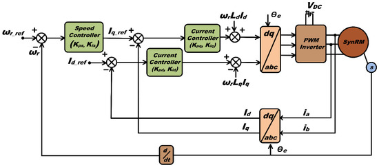
Figure 1.
Speed control of the SynRM in the FOC frame.
The cascaded loop presented in Figure 1 can be analyzed by dividing it into the inner current loop and the outer speed loop. As the PI controller in the current loop generates the required voltage to be induced into the stator winding terminals, the transfer function between Vd (or Vq) and Id (or Iq) is needed to design the PI controller for the inner current loop. Further, to incorporate the computational delays and the inverter delay, the closed-loop current controller is realized as shown in Figure 2.
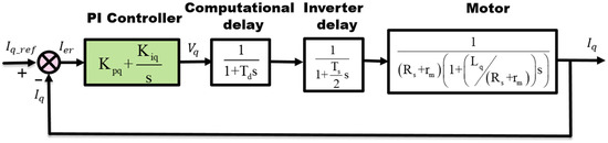
Figure 2.
Closed-loop system diagram of inner current control in Q-axis.
The transfer function between Id and Vd is also derived as with Equation (5), and is given as below:
As the sampling time of the inner current loop is 10 times faster than the outer speed loop, the outer loop is designed with the assumption that the current command always reaches its steady state. Further, by neglecting the load torque and velocity friction terms, the closed loop for the speed control loop is derived from Equations (3), (4) and (6), as shown in Figure 3.
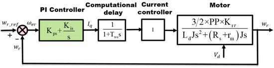
Figure 3.
Closed-loop system diagram of outer speed control loop.
The transfer function between ωr and Iq, after substituting Vd from Equation (6), is computed as prescribed below:
where Krτ () is considered as equivalent reluctance torque constant. The transfer functions derived in Equations (5)–(7) can be used for the PI controller tuning procedure, provided that there is no change in parametric variations in the above equations. However, due to the simultaneous effect of Id and Iq with the cross-magnetization effect on Lq and Ld, variations occur in the magnitudes of the stator inductances [7]. Furthermore, the value of Vd changes which in turn changes the value of Krτ for different operating points. Thus, the usage of the nominal transfer function alone in the PI controller design procedure causes poor tuning. To incorporate these parametric variations, as well as the unmodeled dynamics, and tune a robust control system with a simple structure, QFT is the most suitable design procedure among the available robust control design methods in the frequency domain. Because it preserves the transfer function of the nominal plant, maintaining its simple linear function, it creates a set of multiple linear plants so that the change in the operating point, due to the nonlinear behavior of the parameters, falls within this set of plants. The creation of these multiple plants is further explained in Section 4. The range of parametric variation of the magnitude values of Lq and Ld is properly chosen so that the operating point always falls within the set of multiple plants resulting from the discrete values of the parametric range. Thus, to choose the range of inductance variation, an offline test is conducted on the SynRM using an autotransformer to measure the various Lq and Ld values at different currents, as shown in Figure 4 [26]. Based on the minimum and maximum values of each parameter, a range of parametric variation has been chosen and tabulated as shown in Section 4.
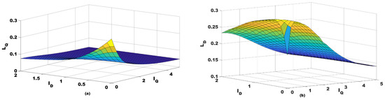
Figure 4.
Variation of (a) Lq and (b) Ld values for variation in currents.
3. QFT Method and FPA Algorithm
This section briefly introduces the terms needed to understand the QFT design procedure. The manual loop shaping of QFT bounds requires good knowledge of control theory; thus, the loop shaping is carried out with the optimization tool.
3.1. QFT Method for PI Tuning
QFT is a frequency domain-based control design method for the quantitative design of closed-loop control systems for the control specifications of a specified magnitude in a specified frequency range [27,28]. The design procedure for QFT generally follows the following steps:
- For a given plant (G(s)), specify the performance indices of the closed-loop control system for the required closed-loop stability and tracking performance [29].
- Describe the transfer function of the nominal model along with the uncertainties, such as the parametric variations and unmodeled dynamics. This illustration provides a set of multiple plants along with the nominal plant.
- Draw the templates by plotting the set of multiple plants in a gain vs. phase plot at the specified discrete frequency set. These templates are useful for observing the variations in phase and magnitude of the transfer function caused by the uncertainties in the plant [30].
- Plot the QFT bounds for all of the controller specifications mentioned in step 1 and draw the intersection of all these bounds in a Nichols chart so that it can represent the worst-case scenario for the set of multiple plants.
- Perform the loop shaping by adding the PI controller (C(s)) to G(s), such that the open loop, L(s) (=G(s)C(s)), should satisfy all bounds plotted for the worst-case scenario in step 4.
- Once the L(s) satisfies all the bounds on the Nichols chart, derive the PI controller from L(s) through L(s)/G(s) [31].
Further detailed information on the design procedure of QFT is illustrated in [15].
3.2. Flower Pollination Algorithm
FPA is a biological nature-inspired evolutionary algorithm based on the reproduction of flower plants through the pollination of pollen gametes [32]. It is a meta-heuristic-type algorithm in which solutions are updated based on the Levy distribution function. The flow of the algorithm is as follows:
- The pollens (as solutions) are uniformly distributed in the search space at the initial iteration. Before the initiation of each iteration, a random value is assigned to the switching probability variable (ρ). Variable ρ is the decision variable for switching the algorithm between the local and global search for a given pollen.
- If pollen is selected for the global search, the algorithm first calculates the strength of pollination using the Levy distribution function for the long flight distances as follows:where the step variable is the domain over which the Levy distribution function is defined and is used to calculate the final value of L, the Levy flight step size. Thus, the update to the pollen’s position (i.e., solution), in a global search, can be represented as:where is ith solution (pollen) at iteration k and is the best solution among all pollens until the kth iteration.
- If a pollen is selected for the local search, the update step for flower constancy, ε, is selected for each solution from a uniform distribution in the interval [0, 1] and the updated solution is given as below:where the jth and lth solutions are chosen randomly from the available n solutions.
- After the update of the pollens, from Equation (9) or (10), the fitness function is evaluated to select the best solution for next iteration, and the next iteration starts again from step 1.
4. Selection of Control Specifications for QFT Method
The QFT procedure provides the combined representation of plant uncertainties and control specifications in a single pictorial graph, in the form of bounds, to synthesize the robust control for the uncertain plant. As the name suggests, QFT considers each component of the control design procedure quantitatively and precisely to generate the required controller gains for a given plant. However, there is no single straightforward procedure to addresses the selection methodology of control specifications for a given plant [15]. This is a significant drawback when designing the robust controller with the most efficient closed-loop operation. As mentioned in Section 3.1, defining the control specifications is the primary step in QFT, and if specifications are not selected to force the controller to perform at its best, the rest of the QFT procedure will lead to the generation of a poorly tuned controller, no matter how good the design procedure of the QFT is. The authors propose an analytical observation before selecting the controller specifications. The design procedure for a current loop PI controller in Q-axis is explained. The same procedure is applicable for tuning the PI controller for a D-axis current controller and outer loop speed controller.
4.1. Selection of Robust Stability and Performance Specifications
Consider the nominal plant mentioned in Equations (5)–(7) as Go(s), with the plant uncertainties and parametric variations as shown in Table 1. These uncertainties will create a set of linear plants called G(s). This set of plants, due to the range of parameters mentioned in Table 1, are incorporated into the variation of the operating point caused by the nonlinearities and other unmodeled dynamics in the nominal linear transfer function. Assume the synthesized PI controller, C(s) from QFT, as below:

Table 1.
SynRM nominal model parameters and their parametric uncertainties.
In order to define robust stability, the values of the phase margin (P.M.) and gain margin (G.M.) have to be specified. Further, to describe the tracking performance specifications, the closed-loop bandwidth (B.W.) needs to be mentioned. The closed-loop systems need these three parametric magnitudes (P.M., G.M., and B.W.) to be as high as possible. To specify these three parametric magnitudes in QFT design and to force them to reach their bottlenecks with a given plant, a systematic procedure in the frequency domain is performed as follows.
Assume there exists a PI controller for Q-axis current control, and that its magnitude and phase at each frequency, from Equation (11), is given as below:
To obtain the G.M. and P.M., the PI controller in Equation (12) has to convert into magnitude and phase loci and then solve at each frequency, ω. Thus, Equation (12) is rewritten as:
where:
According to Equation (13), it is clear that the magnitude locus represents an ellipse and the phase locus represents a straight line. Thus, the intersection point of these two curves for any frequency, ω, represents the phase and magnitude of the PI controller and that the frequency, ω, becomes the bandwidth (B.W.) of that PI controller provided to the system, provided that the intersection point, i.e., the KP and KI values, is in a stable region. This region can be found by solving the closed-loop characteristics equation given by G(s) and C(s) (at the intersection point), as shown in Figure 5. The final G.M. and P.M. are given by Equation (15):
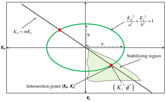
Figure 5.
PI controller magnitude, phase locus along with stable region.
The maximum achievable P.M. and G.M. are examined by solving the intersection points in the KP − KI plane for a particular interval of phase values () at each specified discrete B.W. frequency ().
The loci of the stable intersection points, from Figure 5, are drawn for different frequencies of in the G.M. vs. P.M. plane, so that the P.M., G.M., and B.W are selected for defining the control specifications. For the Q-axis current PI controller, with and at 100 rad/s as a discrete step size, the phase and gain margin curves have been drawn as shown in Figure 6. From the observation of the plot, for example points a and b, it is clear that there is a tradeoff among the three variables. Moreover, there are cases that fail to attain the required P.M., especially at high B.W. frequencies. The high P.M. ensures that the uncertainties are more robust, and so the authors preferred to choose point a as the desired one. Thus, the chosen values for P.M., G.M., and B.W. are 80°, 35.2 dB, and 400 rad/s, respectively. However, the B.W. limit has been relaxed slightly and changed to 350 rad/s so that these performance indices can be ensured, even for the worst-case scenarios caused by the multiple plants due to the plant uncertainties in the QFT method.
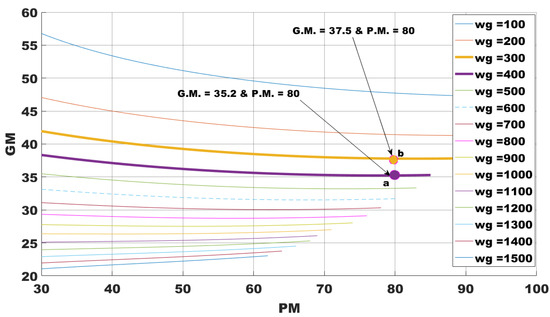
Figure 6.
GM versus PM plot for selecting the robust stability specs.
4.2. Selection of Intial Search Space for FPA Algoirthm
To initialize the pollens in the FPA algorithm, the authors examined the range of stable PI values so that only the stable set of PI values can be fed into the optimization algorithm. To find the stable set of PI values for a closed loop, a certain range of Kp values were initiated and plotted in Figure 5, using Equation (13). The stability of these intersecting points (Kp, KI) is examined using a closed-loop characteristic equation, so that a set of PI values is verified as stable controller gains for the given plant. Thus, for the Q-axis current loop, KP values are initiated in the range of 0 to 200 to find the intersecting points (KP, KI) to identify the stable region of PI values, as shown in Figure 7. This process helps to define the search space for KP as [0, 196] and for KI as [0, 2650].
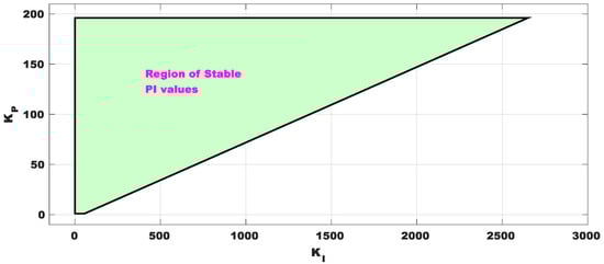
Figure 7.
Stable PI values to initialize the FPA search space.
5. Automatic Loop Shaping QFT Using FPA for PI Design
The nominal plant Go(s) along with the plant uncertainties form the QFT bounds with the control specifications as mentioned in Section 4. Thus, the design procedure for the Q-axis PI controller is as follows:
- Define the discrete set of frequency points at which the QFT design procedure is conducted. For the current case, 12 discrete frequency values are chosen in the range of [1 rad/s, 31,416 rad/s].
- To define robust stability, the limit to the closed-loop transfer function, εs, is selected from the P.M. value, i.e., 80° as shown below:
- The sensitivity function weight Ws is chosen as shown in Equation (17) for a maximum sensitivity (Ms) set to 1.2 and B.W. = 350 rad/s:
- All closed-loop specifications and plant uncertainties are plotted in the Nichols chart as bounds for the worst-case scenario. Thus, the loop shaping need to be performed to satisfy these bounds at all frequencies.
- The automatic loop shaping is performed by initializing the search space with the range of PI values selected in Section 4.2. The other parameters used in the FPA algorithm are shown in Table 2.
Table 2. SynRM nominal model parameters and their parametric uncertainties.
- The multi-component objective function has been used for automatic loop shaping. The fitness function used in Equation (18) is formulated to minimize the distance between the L(s) and QFT bounds, and hence the magnitude of PI gains, as given below:where α is the weighting coefficient with a value of 0.5 to give equal priority in the objective function.
- The synthesized PI controller for Q-axis current regulation is given by Equation (19) and its loop shaping on the Nichols chart to satisfy QFT bounds is shown in Figure 8:
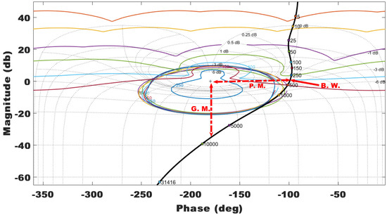 Figure 8. Automated loop-shaping QFT using FPA optimization.From the figure, it is evident that with only two gain variables, the loop shaping is tightly performed at each discrete frequency. The P.M., G.M., and B.W. for even the worst-case scenario are 82°, 36.58 dB, and 386 rad/s, respectively. This ensures that the design procedure not only systematically chooses the control specifications to force the PI controller performance to its bottleneck, but it also ensures that the synthesized controller absolutely satisfies the chosen control specifications in the design procedure.
 - The PI controllers for the D-axis current loop and the outer speed loop are synthesized using a similar procedure, and are presented as given in Equations (20) and (21), respectively:The synthesized PI controllers are discretized using the forward Euler method before being implemented in the MATLAB/Simulink simulation environment.
6. Results and Discussions
The proposed design procedure is validated using MATLAB/Simulink with a fixed step solver environment. The parameters used in the simulation are tabulated in Table 3. The computational delay (Td) can be neglected for high clock frequency processors.
Table 3.
Simulation model parameters for the speed control of a SynRM.
The sampling time for the speed control loop is 1 ms, whereas that of the current loop is 0.1 ms. To compare the effectiveness of the proposed design method, the gains of the PI controllers are tuned from the conventional method given in [34]. The PI controller gain pairs {KP, KI} for the inner current loop are {8.6, 215} and for outer speed loop are {1.2, 4.5}. The iron losses are also incorporated in the model-based simulation. Further, the variation in the Ld and Lq magnitudes, due to the variation in the Id and Iq currents, are realized in the simulation using look-up tables.
6.1. Robust Regulatory Performance
Prior to performing the MATLAB simulation, a comparative frequency response for the disturbance rejection of the closed-loop control was analyzed using a Bode plot. As shown in Equation (17), a sensitivity function is formulated using the plant transfer function, as given in Equation (5), for both of the current PI controllers. These two sensitivity functions are plotted in the Bode plot as shown in Figure 9. The proposed PI controller, clearly, has a high negative magnitude at the lower frequency region of the Bode plot, which proves that the proposed PI control experiences more attenuation to the low frequency signals, such as disturbance signals.
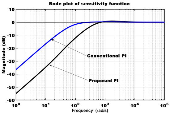
Figure 9.
Comparative Bode plot of sensitivity function.
To verify the regulatory performance/stability of the designed closed-loop speed control in the MATLAB simulation environment, the SynRM drive is initially allowed to reach its steady state speed at 900 min−1. Then, a step change in load from 0.1 Nm to 0.3 Nm (the load torque is increased by 200%) is applied to the motor at time 2 s as an output disturbance.
The closed-loop control designed by the FPA-based QFT method quickly regulates the speed variable to its steady value compared to that of a conventional PI controller. As shown in Figure 10a,b, the inner current PI controller regulates the Iq and Id currents to their steady state values to generate the required torque needed for the reference speed variable.
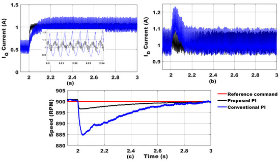
Figure 10.
Comparison of robust regulatory performance of SynRM drive: (a) Regulation of Iq currents to their desired Iq values, (b) Regulation of Id currents to their desired Id values, (c) Regulation of speed variables, under load torque disturbance.
These figures also illustrate that the proposed method has less ripple in the controlled Iq and Id current waveforms than the conventional method. As the fundamental frequency of the ripple also falls within the low frequency region of the sensitivity function, as mentioned in Figure 9, the proposed PI controller attenuates the steady state ripple in the current waveforms. This, in turn, causes the low ripple in the speed variable, which is low compared to that of the conventional speed controller, as observed in Figure 10c. From all three figures in Figure 10, along with Figure 9, it is observed that the design procedure for the PI controller’s gains, based on the QFT bounds that involve the sensitivity function, reflects the maximum deviation of the controlled variables while regulating their steady state values in the presence of the external disturbance. Thanks to the G.M. versus P.M. plot, drawn from the analytical method, we are able to choose an appropriate B.W. value to be used in the sensitivity function for a specified P.M. and G.M.
6.2. Robust Tracking Performance
To validate the tracking performance of the SynRM drive, a sudden step change of 600 min−1 to 900 min−1 is given to the reference speed command. As shown in Figure 11, both of the closed-loop PI controllers settle the speed variable with an almost similar settling time and peak overshoot, whereas the proposed FPA-based QFT closed-loop system tracks the reference speed variable with less rise time compared to that of the conventional PI controller. This exemplifies that the proposed method has succeeded in producing a better tradeoff between stability and the tracking performance indices, with the use of more systematic observations and an automatic tuning procedure to achieve those indices, as mentioned in Section 5. As the proposed PI design includes the variation in Ld and Lq, the change in Ld and Lq values due to the change in Id and Iq during the transient conditions are less sensitive to the effect of the controlled variables, such as the speed command. The tracking performance of the proposed closed-loop speed control is thoroughly verified at low, medium, and high speed ranges, as shown in Figure 12.
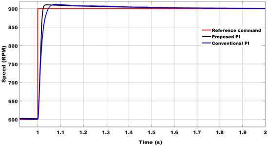
Figure 11.
Comparison of robust tracking performance of SynRM drive under the step change of speed command.
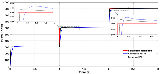
Figure 12.
Comparison of robust tracking performance of SynRM drive at various speed ranges.
To further gauge the performance of the proposed method compared to the conventional method, the IAE (integral absolute error) of the speed variable is tabulated in Table 4 for both the conditions shown in Figure 10 and Figure 11. These IAE indices are calculated for the time interval starting from their transient initiation instant to the end time shown in the respective figures. The values for the IAE clearly indicate the better performance of the proposed method over the conventional method.
Table 4.
Comparative IAE values for regulatory and tracking performances of the closed-loop SynRM drive.
6.3. Robust Performance to the Parametric Variations
To check the PI controller’s performance under the effect of parametric variations on the controlled variables, such as Iq and speed, the change in the magnitudes of Ld, Lq, and iron losses (rm) are incorporated into the simulation. As mentioned earlier, the change in Ld and Lq are mentioned in terms of Id and Iq. The Iq current changes very widely during the transient conditions of change in the speed command to create the necessary torque for the acceleration. Hence, the magnitude of Ld and Lq changes significantly in this vicinity. Thus, the current control performance of the PI controller is examined in the interval at which the speed changes from 600 to 900 min−1, as mentioned in Section 6.2. The Iq error, in Figure 13a, shows the deviation of the actual current waveform from its reference signal. This confirms that the designed QFT-based PI is less sensitive than that of the conventional PI for the change in Ld and Lq values during that transient period. To validate the robustness of the controller to change in the iron losses of the SynRM, the speed regulation is observed at 900 min−1 for the change in iron losses corresponding to variation of Krm from 5 mΩ/(rad/s) to 15 mΩ/(rad/s), at time 3 s. Figure 13b demonstrates that the QFT-based PI Controller regulates the speed variable faster than the conventional PI in the presence of changes in iron losses.
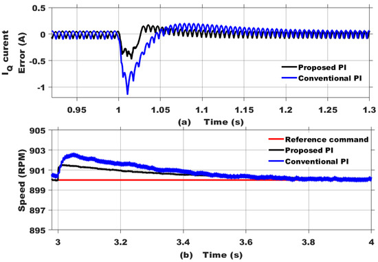
Figure 13.
Comparison of robust regulatory performance of SynRM drive under the parametric variations: (a) current regulation under Ld and Lq variation, (b) speed regulation under iron losses variation.
As the proposed method uses the MATLAB simulation environment, it is easy to realize the step change in iron loss of SynRM compared to the experimental setup. However, the present simulation further needs to be verified using a real-time simulation environment or a hardware prototype.
7. Conclusions
A method is developed to design a PI controller in the fully analytical frequency domain for robust speed control against parametric variations that affect SynRM drives, such as changes to Ld and Lq, armature resistance, and iron losses. The QFT has enabled us to incorporate the nonlinear behavior of the SynRM inductances using the multiple linear plant models that have resulted from the parametric variation in the SynRM. A successful effort has been made to choose the G.M., P.M., and B.W. of the closed-loop control for a given plant model of a SynRM. The initiation of the optimization algorithm, in order to find the best PI gains for tight loop shaping in the Nichols chart, is performed in the search space realized from the stable PI region provided by an analytical frequency domain approach. Thus, this analytical approach, in choosing the control performance specifications and the initial search space for the optimization process, enhances the design transparency of the automated QFT design method. The comparative simulation results illustrate the effectiveness of this approach at forcing the PI controller to achieve a better robust performance for a given plant compared to the conventional design. However, as shown in the result of the tracking performance of speed, the PI controller in the 1-DOF (degree of freedom) scheme is unable to provide its best tracking performance, which paves the path for a 2-DOF scheme that will perform better when making tradeoffs between the simultaneous regulatory and tracking performances.
Author Contributions
The whole work was carried out by R.P. under the supervision of T.H. However, the modeling of the Ld and Lq variations in the function of Id and Iq was also created by Tsuyoshi Hanamoto. All authors have read and agreed to the published version of the manuscript.
Funding
This research received no external funding.
Institutional Review Board Statement
Not applicable.
Informed Consent Statement
Not applicable.
Conflicts of Interest
The authors declare no conflict of interest.
References
- Ozcelik, N.G.; Dogru, U.E.; Imeryuz, M.; Ergene, L.T. Synchronous Reluctance Motor vs. Induction Motor at Low-Power Industrial Applications: Design and Comparison. Energies 2019, 12, 2190. [Google Scholar] [CrossRef] [Green Version]
- Oliveira, F.; Ukil, A. Comparative performance analysis of induction & synchronous reluctance motors in chiller systems for energy efficient buildings. IEEE Trans. Ind. Informat. 2019, 15, 4384–4393. [Google Scholar]
- Zhu, Z.Q.; Chu, W.Q.; Guan, Y. Quantitative comparison of electromagnetic performance of electrical machines for HEVs/EVs. CES Trans. Electr. Mach. Syst. 2017, 1, 37–47. [Google Scholar] [CrossRef]
- Goman, V.; Prakht, V.; Kazakbaev, V.; Dmitrievskii, V. Comparative Study of Energy Consumption and CO2 Emissions of Variable-Speed Electric Drives with Induction and Synchronous Reluctance Motors in Pump Units. Mathematics 2021, 9, 2679. [Google Scholar] [CrossRef]
- Cai, S.; Jin, M.-J.; Hao, H.; Shen, J.-X.A. Comparative study on synchronous reluctance and PM machines. COMPEL Int. J. Comput. Math. Electr. Electron. Eng. 2016, 35, 607–623. [Google Scholar] [CrossRef]
- Bianchi, N.; Bolognani, S.; Carraro, E.; Castiello, M.; Fornasiero, E. Electric vehicle traction based on synchronous reluctance motors. IEEE Trans. Ind. Appl. 2016, 52, 4762–4769. [Google Scholar] [CrossRef]
- Zhao, Y.; Ren, L.; Liao, Z.; Lin, G. A Novel Model Predictive Direct Torque Control Method for Improving Steady-State Performance of the Synchronous Reluctance Motor. Energies 2021, 14, 2256. [Google Scholar] [CrossRef]
- Boldea, I.; Fu, Z.; Nasar, S. Torque vector control (TVC) of axially-laminated anisotropic (ALA) rotor reluctance synchronous motors. Electr. Mach. Power Syst. 1991, 19, 381–398. [Google Scholar] [CrossRef]
- Matsuo, T.; Lipo, T. Field Oriented Control of Synchronous Reluctance Machine. In Proceedings of the 24th Annual IEEE Power Electronics Specialists Conference, Seattle, WA, USA, 20–24 June 1993; pp. 425–431. [Google Scholar]
- Chikhi, A.; Djarallah, M.; Chikhi, K. A comparative study of field-oriented control and direct-torque control of induction motors using an adaptive flux observer. Serb. J. Electr. Eng. 2010, 7, 41–55. [Google Scholar] [CrossRef]
- Rashad, E.; Radwan, T.; Rahman, M. A Maximum Torque Per Ampere Vector Control Strategy for Synchronous Reluctance Motors Considering Saturation and Iron Losse. In Proceedings of the 2004 IEEE Industry Applications Conference (39th IAS Annual Meeting), Seattle, WA, USA, 3–7 October 2004; Volume 4, pp. 2411–2417. [Google Scholar]
- Hackl, C.M.; Kamper, M.J.; Kullick, J.; Mitchell, J. Current Control of Reluctance Synchronous Machines with Online Adjustment of the Controller Parameters. In Proceedings of the IEEE 25th International Symposium on Industrial Electronics (ISIE), Santa Clara, CA, USA, 8–10 June 2016; pp. 153–160. [Google Scholar]
- Lin, F.; Huang, M.; Chen, S.; Hsu, C. Intelligent Maximum Torque per Ampere Tracking Control of Synchronous Reluctance Motor Using Recurrent Legendre Fuzzy Neural Network. IEEE Trans. Power Electron. 2019, 34, 12080–12094. [Google Scholar] [CrossRef]
- Ramon, V.; Antonio, V. PID Control in the Third Millennium: Lessons Learned and New Approaches; Springer: New York, NY, USA, 2012. [Google Scholar]
- Sanz, M.G. Robust Control Engineering: Practical QFT Solutions, 1st ed.; CRC, Taylor & Francis Group: Boca Raton, FL, USA, 2021; pp. 17–78. [Google Scholar]
- Rigatos, G.; Siano, P.; Wira, P.; Hamida, M. An H-infinity approach to optimal control of doubly-fed reluctance machines. IFAC-PapersOnLine 2016, 49, 116–122. [Google Scholar] [CrossRef]
- Nitish, K.; Shiv, N. Automatic Loop Shaping of Robust QFT Controller for Permanent Magnet Stepper Motor using Flower Pollination Algorithm. Int. J. Control Theory Appl. 2016, 9, 85–94. [Google Scholar]
- Lucas, C.; Shanehchi, M.M.; Asadi, P.; Rad, P.M. A Robust Speed Controller for Switched Reluctance Motor with Nonlinear QFT Design Approach. In Proceedings of the Thirty-Fifth IAS Annual Meeting and World Conference on Industrial Applications of Electrical Energy, Rome, Italy, 8–12 October 2000; pp. 1573–1577. [Google Scholar]
- Xu, Q.; Huang, J.; Li, H. Gravitational search algorithm-based fractional order QFT control scheme for PMSM. In Proceedings of the 32nd Chinese Control Conference, Xi’an, China, 26–28 July 2013; pp. 4442–4445. [Google Scholar]
- Luis, I.; Pedro, P.; Arturo, M. Robust QFT-based control of DTC-speed loop of an induction motor under different load conditions. IFAC-PapersOnLine 2015, 48, 2429–2434. [Google Scholar]
- Kilthau, A.; Pacas, J.M. Appropriate Models for the Control of the Synchronous Reluctance Machine. In Proceedings of the 37th IAS Annual Meeting Industry Applications Conference, Pittsburgh, PA, USA, 13–18 October 2002; Volume 4, pp. 2289–2295. [Google Scholar]
- Liu, T.H.; Ming-Tsan, U.N. A fuzzy sliding-mode controller design for a synchronous reluctance motor drive. IEEE Trans. Aerosp. Electron. Syst. 1996, 32, 1065–1076. [Google Scholar]
- Senjyu, T.; Kinjo, K.; Urasaki, N.; Uezato, K. Sensorless Control of Synchronous Reluctance Motors Considering the Stator Iron Loss with Extended Kalman Filter. In Proceedings of the IEEE 34th Annual Conference on Power Electronics Specialist, Acapulco, Mexico, 15–19 June 2003; Volume 7445, pp. 403–408. [Google Scholar] [CrossRef]
- Dalibor, I.; Amor, C.; Bojan, Š.; Andrej, S. Robust tracking system design for a synchronous reluctance motor—SynRM based on a new modified bat optimization algorithm algorithm. Appl. Soft Comput. 2018, 69, 568–584. [Google Scholar]
- Lin, C. Adaptive recurrent fuzzy neural network control for synchronous reluctance motor servo drive. IEE Proc. Electr. Power Appl. 2004, 151, 711–724. [Google Scholar] [CrossRef]
- Yahia, K.; Matos, D.; Estima, J.O.; Cardoso, A.J.M. Modeling Synchronous Reluctance Motors including Saturation, Iron Losses and Mechanical Losses. In Proceedings of the 2014 International Symposium on Power Electronics, Electrical Drives, Automation and Motion, Ischia, Italy, 18–20 June 2014; pp. 601–606. [Google Scholar]
- Horowitz, I. Synthesis of Feedback Systems; Academic Press: New York, NY, USA, 1963. [Google Scholar]
- Garcia-Sanz, M.; Houpis, C.H. Part I: QFT Control, Part II: Wind Turbine Design and Control. In Wind Energy Systems: Control Engineering Design; A CRC Press Book; Taylor & Francis Group: Boca Raton, FL, USA, 2012. [Google Scholar]
- Longdon, L.; East, D.J. A simple geometrical technique for determining loop frequency bounds which achieve prescribed sensitivity specifications. Int. J. Control 1978, 30, 153–158. [Google Scholar] [CrossRef]
- Ballance, D.J.; Hughes, G. A Survey of Template Generation Methods for Quantitative Feedback Theory. In Proceedings of the UKACC International Conference on Control, Exeter, UK, 2–5 September 1996; pp. 172–174. [Google Scholar]
- Garcia-Sanz, M.; Brugarolas, M.J.; Eguinoa, I. Quantitative Analysis of Controller Fragility in the Frequency Domain. In Proceedings of the UKACC 23rd IASTED International Symposium on Modelling, Identiication and Control, Grindelwald, Switzerland, 23–25 February 2004. [Google Scholar]
- Yang, X.-S. Flower Pollination Algorithm for Global Optimization. In Unconventional Computation and Natural Computation 2012; Lecture Notes in Computer Science; Springer: Berlin/Heidelberg, Germany, 2012; Volume 7445, pp. 240–249. [Google Scholar]
- Valenti, C. Microchip, AN937, Implementing a PID Controller Using a PIC18 MCU. Available online: https://ww1.microchip.com/downloads/en/AppNotes/00937a.pdf (accessed on 14 October 2021).
- Wang, Q.G.; Fung, H.W.; Zhang, Y. PID tuning with exact gain and phase margins. ISA Trans. 1999, 38, 243–249. [Google Scholar] [CrossRef]
Publisher’s Note: MDPI stays neutral with regard to jurisdictional claims in published maps and institutional affiliations. |
© 2022 by the authors. Licensee MDPI, Basel, Switzerland. This article is an open access article distributed under the terms and conditions of the Creative Commons Attribution (CC BY) license (https://creativecommons.org/licenses/by/4.0/).