Article

A Comparative Analysis of Brake-by-Wire Smart Actuators Using Optimization Strategies

Department of Mechanical and Aerospace Engineering, University of California, Davis, CA 95616, USA
*
Authors to whom correspondence should be addressed.
Energies 2022, 15(2), 634; https://doi.org/10.3390/en15020634
Submission received: 18 November 2021 / Revised: 24 December 2021 / Accepted: 7 January 2022 / Published: 17 January 2022

Abstract

:
Since the automotive industry is shifting towards electrification, brake-by-wire technologies are becoming more prevalent. However, there has been little research comparing and optimizing brake-by-wire actuators in terms of their energy expenditure and response time. This paper investigates the comparison of three different smart brake-by-wire actuators, Electro-Hydraulic Brakes (EHB), Electro-Mechanical Brakes (EMB), and Electronic Wedge Brakes (EWB), first by defining an objective metric and then using both linear and nonlinear optimization techniques. Modeling of the actuators is performed using the bond graph method. Then, the controllers are designed using a robust control strategy, Youla parameterization. After designing the controllers, two types of optimization are performed on the actuators. Optimizations are performed in two ways: 1. by linearizing the plants and optimizing using their transfer functions and 2. by nonlinear optimization of the plants in the closed-loop following a specific clamp force target. The objective metrics or the cost functions for these optimizations are chosen to be the energy usage of the plants during the closed-loop operation, maximum power requirement, and their dynamic responsiveness. Using this optimization framework, we can show a significant improvement in the energy usage of the actuators and slight improvements in their responsiveness. In the end, the actuators are compared in terms of their energy usage for sets of initial and optimized physical parameters.

1. Introduction

By-wire technologies are becoming more in demand because of their contribution to the vehicle’s fuel efficiency and electrification. They are well suited for autonomous vehicles, Electric Vehicles (EVs), and Hybrid Electric Vehicles (HEVs) due to their electronic interface and architectures. Between all these by-wire technologies, brake-by-wires are essential since they play a critical role in the vehicle’s safety [1,2,3].
Brake-by-wire systems can reduce the overall component weight due to the reduction in the number of parts and integrated packaging. They also improve energy consumption because they would only use energy when required. The reduction of energy usage by different components is an essential aspect of reducing the CO 2 emissions of vehicles. This type of reduction is significant in reducing fleet CO 2 emissions. When the brake pedal is released, the brake pad may not release entirely, causing caliper drag. Brake-by-wire is even more energy-efficient by eliminating caliper drag through sensors and control methods. To enhance vehicle safety, individual wheel braking and faster activation times of BBW actuators can be utilized by the vehicle’s Electronic Stability Control (ESC) system. The biggest barriers to brake-by-wire systems gaining popularity in the automotive industry are the reliability of new actuators, as well as the risk and cost of deploying new braking technology [4].

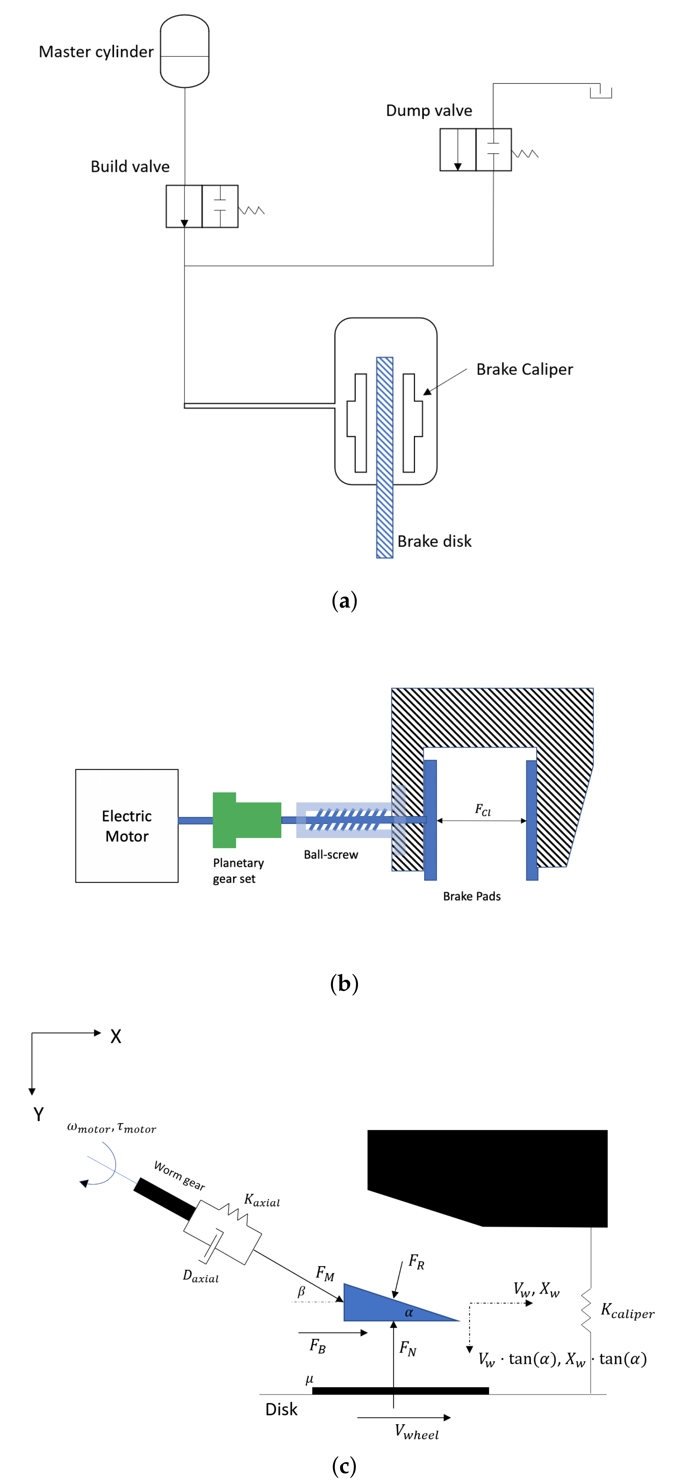
1.1. Brake-by-Wire Actuators

Wet and dry brakes are the two types of braking systems. Dry brakes are simply mechanical systems that rely on electric motors, whereas wet brakes employ fluids to produce pressure on the piston and the caliper. A type of wet brake is electro-hydraulic brakes, which include solenoid valves that can be operated with an electronic signal to vary the braking pressure. These types of brakes require an accumulator and a pump, and usually a vacuum booster to maintain their high pressure throughout the braking operation. There are also a few different types of dry brakes. In a pure electro-mechanical brake, a small electric motor, planetary gear set, and roller screw energizes the brake pad [5,6,7,8]. For this type of brake, however, a 42 volt motor is needed, which is energy intensive [4]. On the other hand, a wedge mechanism is used in electronic wedge brakes to create a brake caliper, which is drawn into the brake and uses less energy because it utilizes the wheel’s rotation. They usually need a 14 V supply as opposed to the 42 V of the electro-mechanical brake. However, this comes at the cost of more complicated mechanics and control [5,8,9,10,11,12,13,14,15,16]. Vienna Engineering has created a brake system based on a crank-shaft mechanism that reduces the complexity of dealing with the reduction gears and roller screws [17].
Purely dry brakes are expensive compared to conventional electro-hydraulic brakes since they are new technologies and need more testing and research before they can be reliable enough to go into production. The reliability of purely dry brakes is a challenge since they have more electronic components, and these components need to work reliably in an environment where vibration, shock, and temperature can significantly affect their nominal performance [4].
On the other hand, EHBs have been used by manufacturers for a while. For example, an integrated electro-hydraulic brake system utilizes an electro-mechanical actuator (similar to an electro-mechanical brake) as a modulator of a master cylinder. This electro-mechanical actuator uses a motor to rotate a gear mechanism and a ball-screw that pushes the piston. This axial force pressurizes the brake fluid inside the master cylinder. The pressurized brake fluid is then transferred to the wheel chamber using a high-pressure pipeline, where this pressure displaces the caliper (similar to an EHB). This integrated electro-hydraulic brake uses most of the EHB parts that the automotive manufacturers are already familiar with and removes the need for a pump, vacuum booster, and accumulator [18,19]. It also seems that this type of brake actuator is gaining popularity among car manufacturers. Bosch GmbH developed the iBooster and ESP hev (electronic stability program for hybrid and electric vehicles), which are integrated electro-hydraulic and Hydraulic Control Units (HCU) in 2013. In 2017, Continental AG introduced MK C1, which is an integrated EHB with fast actuation and without any vacuum booster or accumulator along with emergency brake functionalities [20]. ZF TRW (with the IBC) and Hyundai Mobis (with iMEB) are among the more recent suppliers who developed and manufactured integrated electro-hydraulic brake actuators.

1.2. Objective Metrics for Brake-by-Wire Systems

Objective metrics are required for performing a comparative analysis of the systems under consideration. These metrics are utilized to measure each system’s performance, robustness, and safety correctly. Similar metrics have already been used in other automotive applications to optimize or compare different topologies (different configurations). For example, Shankar et al. use several criteria for optimization and component sizing of plug-in hybrid electric vehicles. The objective functions in their optimization include all-electric range (AER), the CO2 emission from the drive-cycle, and the cost of components [21].
Gombert et al. provide some basic metrics for brake-by-wire actuators and their vehicle configurations [4]. They provide some background for the objective metrics that need to be considered for Brake-By-Wire (BBW) actuators. Yao et al. consider a multi-objective optimization with a few constraints for their combined electromagnetic and electronic wedge brake-by-wire actuator. The objective comprises a time to braking at an acceptable slew rate, maximum initial braking torque, and electric power of the DC motor. Their constraints include the maximum power of the DC motor, brake slew rate, and maximum braking torque (maximum ground friction coefficient) [22,23]. Kwon et al. use a multi-objective formulation to optimize a caliper for the wedge brake. Their objective function includes the minimization of weight and the maximization of caliper stiffness. They then use the response surface model to optimize and find the best possible set of caliper parameters [24].
Metrics and metric-based optimization have also been used in the control architecture of brake-by-wire systems. Fengjiao et al. use multi-objective optimization for their control strategy of an electro-hydraulic brake system in an EV. Their objectives include 1. braking stability, which can be expressed as a quadratic function of friction adhesion on the rear and front wheels and the brake input, and 2. regenerative energy recovery. The constraints include battery charging power, motor peak torque, and the relationship between vehicle stability while braking and road surface friction [23]. Hielinger et al. used parameter optimization for an autonomous emergency braking system. Their cost function includes safety performance and customer acceptance. Safety performance is measured as the reduction of the impact speed (the speed at which the vehicle might collide to the nearest obstacle; if there is no collision, the cost becomes zero). Customer acceptance includes a sub-cost function for the brake profile (the deceleration of the vehicle summed over time) and braking the distance (minimum distance between the vehicle and the obstacle) [25]. Kelling et al. studied a distributed electronic and control architecture design for brake-by-wire systems and compared a conventional centralized architecture with a proposed fault-tolerant and distributed system in terms of safety and cost advantages [26].

1.3. Control Strategies for Brake-by-Wire Systems

Many researchers have used the sliding mode method to control the wheel slip for Anti-Lock Braking (ABS). Sliding Mode Controller (SMC) is a nonlinear control technique and an inherently non-continuous control law, which requires additional filtering to suitably smooth out this discontinuous control law, to force the system to operate on a sliding surface which defines the system’s closed-loop dynamic. Compared to bang-bang control, SMC has the benefits of smaller actuation and added robustness. Anwar utilized a sliding mode controller to control slip in a hybrid BBW system that resulted in a good slip regulation in low friction surfaces and a smooth operation of the ABS, and reduced noise, vibration, and harshness (NVH) in EHB systems [27]. Tanelli et al. use pseudo-sliding mode control combining slip-deceleration (MSD), which continuously controls slip and deceleration while avoiding chattering and is robust against measurement noise and low sampling frequency [28]. However, SMC is not widely used in the automotive industry due to its design complexity, calibration difficulties, proper consideration of actuator delays, and difficulties with addressing robustness. Actuators have delays that can make the sliding mode lead to chatter, energy loss, and the excitation of unmodeled dynamics. However, this is not as much of a problem in the continuous control design [29]. Soltani et al. use a linearized model of EHB and synthesize closed-loop shaping Youla parameterization for the wheel slip control. The stability and performance of the controller were tested on an HiL (hardware in the loop) setup [30].

1.4. Contribution and Paper Structure

This paper discusses a novel approach to optimize three different brake-by-wire actuators. The novelty of this paper is as follows:
  • To the best of the authors’ knowledge, this is the first paper on the optimization and comparison of brake-by-wire actuators’ energy usage and responsiveness;
  • Use of transfer functions as a way to optimize a nonlinear plant;
  • The optimization of the brake-by-wire actuators operating in closed-loop (and following a target) has not been investigated before;
  • The use of a robust control method (Youla parameterization) to control an EHB brake with build and dump valves (the use of Youla parameterization for EMB and EWB has already been investigated in another paper by the authors [31]);.
The structure of this paper is as follows: In the materials and methods section, the procedures used to achieve the results are discussed. The actuator modeling subsection discusses how each actuator has been mathematically modeled. The model-based control synthesis subsection discusses the robust control design. The optimization section discusses the transfer function and nonlinear plant optimization. In the section results and discussion, the optimization results are presented and discussed. Moreover, in the final section, the conclusions, the final conclusion is drawn, and the benefits and the pitfalls of the optimization framework are discussed.

2. Materials and Methods

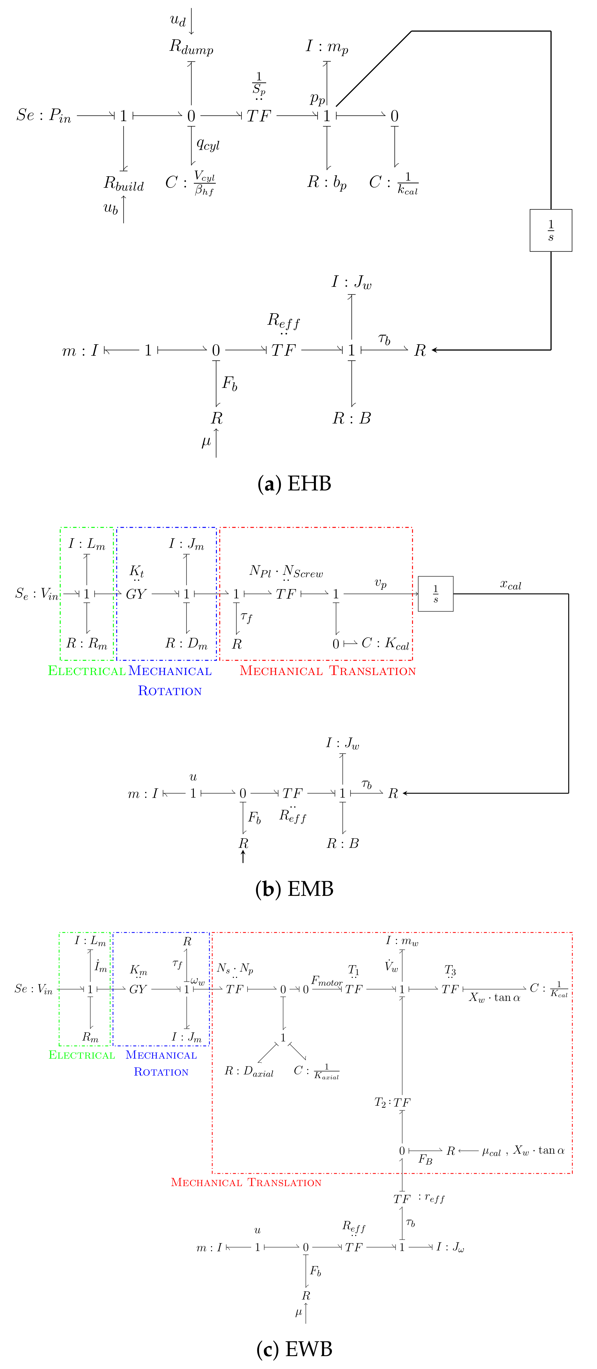
2.1. Actuator Modeling

The schematics of EHB, EMB, and EWB brakes are shown in Figure 1a–c.
EHB model consists of a high-pressure source (master cylinder), hydraulic lines, build and dump valves, a brake cylinder chamber, and brake pads. The master cylinder provides pressure into the high-pressure line, controlled by the build and dump valves. Build and dump valves are considered to have varying states between their fully open and fully closed states. This is as opposed to the valves that can either be fully open or fully closed at a given time. In practice, these are solenoid valves that can be controlled with pulse width modulation. For the sake of initial comparison between these smart brake actuators, a vehicle model containing only one-wheel is utilized. When the pressure increases in the brake cylinder chamber, this pressure will move the brake pad forward. This forward movement of the braking pad stops the brake disk as a result. Upon stopping, the dump valve opens, decreases the pressure, and releases the brake pads, bringing them back to their original position.
The EMB comprises a small electric motor, planetary gear set, ball-screw mechanism, brake pad, and caliper. A planetary gear set and a ball screw mechanism move the brake pad when the motor rotates. This movement will result in a clamp force that is denoted by F c l as illustrated in Figure 1b.
The EWB actuator converts the motor’s rotation to a linear force on the wedge by using a planetary gear set (not depicted in the schematic) and a roller screw. The motor shaft’s axial stiffness and resistance are also considered in modeling this actuator. K c a l represents the combined caliper stiffness and the stiffness between the wedge and the disk. This is similar to the EMB configuration, except that the caliper is shaped like a wedge, which, by inserting it inside the brake casing, creates a self-reinforcing mechanism.
Bond graph is a graphical modeling approach for dynamical systems based on the flow/exchange of power, and therefore, energy. Among the many benefits of bond graphs, they are suitable for the systems with multiple energy domains such as mechatronic systems that usually include various electronic, electrical, mechanical, and hydraulic components [32]. Bond graphs are multi-energy domain and open architecture, which means one can easily add and expand the models with minimum effort compared to other modeling techniques. Furthermore, the monitoring and processing power and energy consumption of various components and parts are conducted with ease when using bond graphs. Given the mentioned benefits of this modeling technique, this method is adopted here to study and model BBW systems.
Figure 2a–c show the bond graph of EHB, EMB, and EWB, respectively. A one-wheel vehicle model is included in all the actuator bond graph models. The wheel has rotational inertia and is connected to a point mass. For the preliminary studies of brake actuators and their algorithms (for example, the Anti-Lock Braking System, ABS, and Traction Control System, TCS), this simple one-wheel model can be used and is easy to implement later on a hardware-in-the-loop test. Models such as this can be used for studying longitudinal dynamics in the vehicle. Since it focuses only on the longitudinal dynamics of the vehicle, it is perfectly suited for studying brake-by-wire actuators and ABS technologies [34].
Based on the bond graphs in Figure 2a–c, the equations of motion for EHB, EMB, and EWB can be written. Equations (1)–(4) represent the equations of motion for the EHB. q c y l , p p , x c a l , P i n , u b , and u d are the volumetric displacement of the cylinder fluid, momentum of the caliper, caliper displacement, pressure of the master-cylinder (high pressure input), duty ratio of build valve, and duty ratio of dump valve (between 0 and 1), respectively.
C d , S b , S d , ρ , β h f , V c y l , S p , b p , m p , x 0 , and k c a l are the maximum flow coefficient of the valve, cross-sectional area of the build valve when fully open, cross-sectional area of the dump valve when fully open, density of the brake fluid, bulk modulus of the brake fluid, cylinder’s volume, cylinder’s cross-section surface, damping coefficient, brake pad’s mass, brake clearance, and caliper stiffness, respectively [33]. Since these equations are highly nonlinear because of the valves, a linearized version, for the purpose of control development, is given in Equations (5)–(7). In this linearization, it is assumed that u d = 1 u b , and this means that when one valve is open, the other is closed.
EHB equations of motion are as follows:
q ˙ c y l = C d S b u b 2 ρ ( P in β h f V c y l q c y l ) C d S d u d 2 ρ ( β h f V c y l q c y l ) S p m p p p
p ˙ p = S p β h f V c y l q c y l b p p p m p k cal max ( x c a l x 0 , 0 )
x ˙ c a l = 1 m p p p
P c y l = β h f V c y l q c y l
Linearized EHB equations are as follows:
A = C d S b u 0 1 2 ρ β h f V c y l ( P i n β h f V c y l q c 0 ) C d S d ( 1 u 0 ) 1 2 ρ β h f V c y l 1 q c 0 S p m p 0 S p β h f V c y l b p m p k c a l 0 1 m p 0
B = C d S b 2 ρ ( P in β h f V c y l q c 0 ) + C d S d 2 ρ ( β h f V c y l q c 0 ) 0 0
q ˙ c y l p ˙ p x ˙ c a l = A q c y l p p x c a l + B u b
Similarly, equations of motion for the EMB can be written using Equations (8a)–(8d). Note that the same nonlinear friction model has been used for the EMB and EWB models. I m , V i n , and ω m are current, voltage input, and angular velocity of the shaft, respectively. L m , R m , K t , J m , D m , N s , N p , and K c a l are the inductance of the electric motor, electrical resistance, electromotive force constant, total moment of inertia of the rotational parts (including the shaft and gears), axial viscous friction, planetary gear reduction ratio, ball-screw gear reduction ratio, and caliper stiffness, respectively.
EMB equations of motion are as follows:
I ˙ m = 1 L m × ( V i n R m × I m K t × ω m )
ω ˙ m = 1 J m × ( K t × I m D m × ω m τ f N p × N s × K c a l × max ( X c a l x 0 , 0 ) )
X ˙ c a l = N s × N p × ω m
F C a l = K c a l X c a l x 0 , if X c a l x 0 0 , otherwise
Equations (9a)–(9h) show the equations of motion for the EWB, where N, q a x , K a x , D a x , X w , V w , F m , α , and μ c a l are combined gear reduction, shaft axial displacement, shaft axial stiffness, shaft axial viscous resistance, wedge displacement, wedge velocity, motor force exerted to the wedge, wedge angle, and friction coefficient between the pad and the wheel, respectively.
EWB equations of motion are as follows:
I ˙ m = 1 L m × ( V i n i m × R m K m × ω m )
q ˙ a x = L N ω V w cos ( α )
F m = K a x q a x + D a x q ˙ a x
ω ˙ = 1 J m { K m I m D m × ω τ f L × N × F m }
V ˙ w = 1 m w ( 1 + tan 2 ( α ) ) × { F m cos ( α ) + ( K c a l × X w × tan ( α ) × ( μ c a l tan ( α ) ) }
X ˙ w = V w
F B = μ c a l K c a l X w tan ( α )
F C a l = K c a l X c a l x 0 , if X w x 0 0 , otherwise
τ f is the lumped nonlinear frictions present in the shaft, planetary gears, and worm gear. The Lugre friction model has been used to model this nonlinear friction. The Lugre model is used for modeling the frictions in actuators since it offers a dynamical model which captures the dynamics very well while needing a lower number of parameters. Other types of friction models can be used as well to represent the frictions. Equation (10a) represents the Lugre friction model [35] where σ 0 , σ 1 , σ 2 , ω s , j, τ c , and τ s are the contact (bristle) stiffness, damping coefficient of the bristle, viscous friction coefficient, Stribeck velocity, shape factor, Coulomb friction, and static friction, respectively. Equation (10d) shows that there is a linear relationship between the Coulomb friction and the clamping force, which is usually derived through experiment. As clamping force increases, the normal forces inside the gears increase as well, which results in increasing the friction torque [6].
Lugre dynamic friction model for EMB and EWB is as follows:
g ( v ) = τ c + ( τ s τ c ) × e | ω ω s | j
z ˙ = ω σ 0 × ω × Z g ( v )
τ f = σ 0 × z + σ 1 × z ˙ + σ 2 × ω
τ c = C + G × F C a l

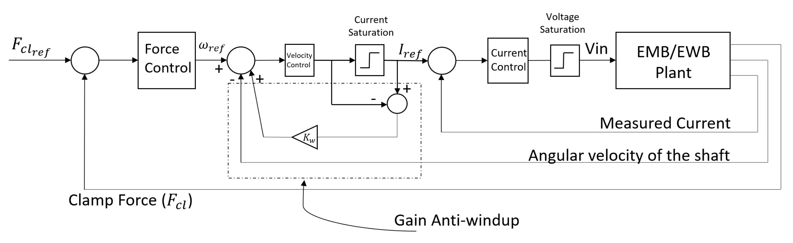
2.2. Model-Based Control Synthesis
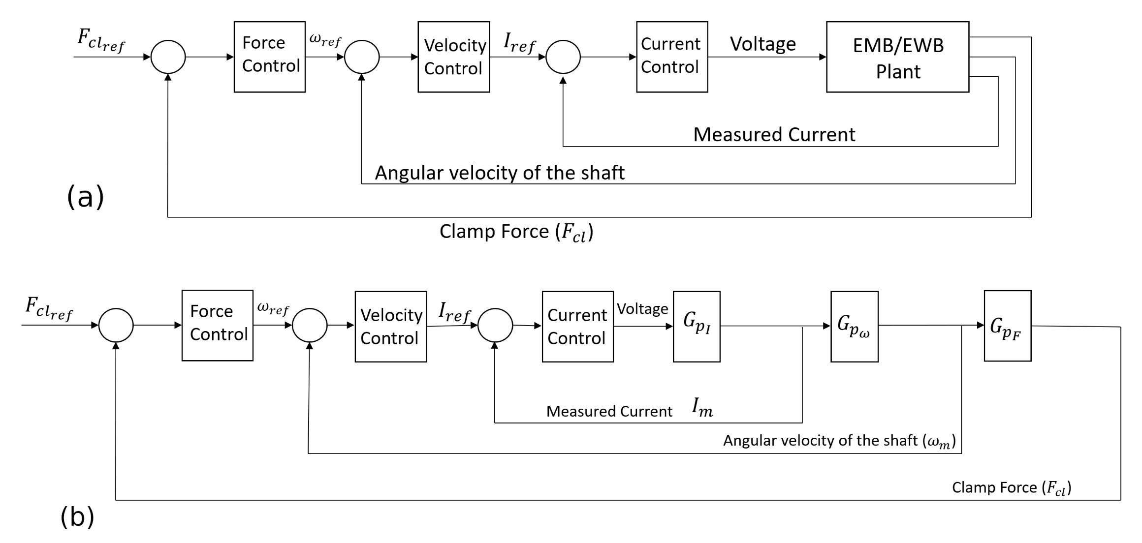
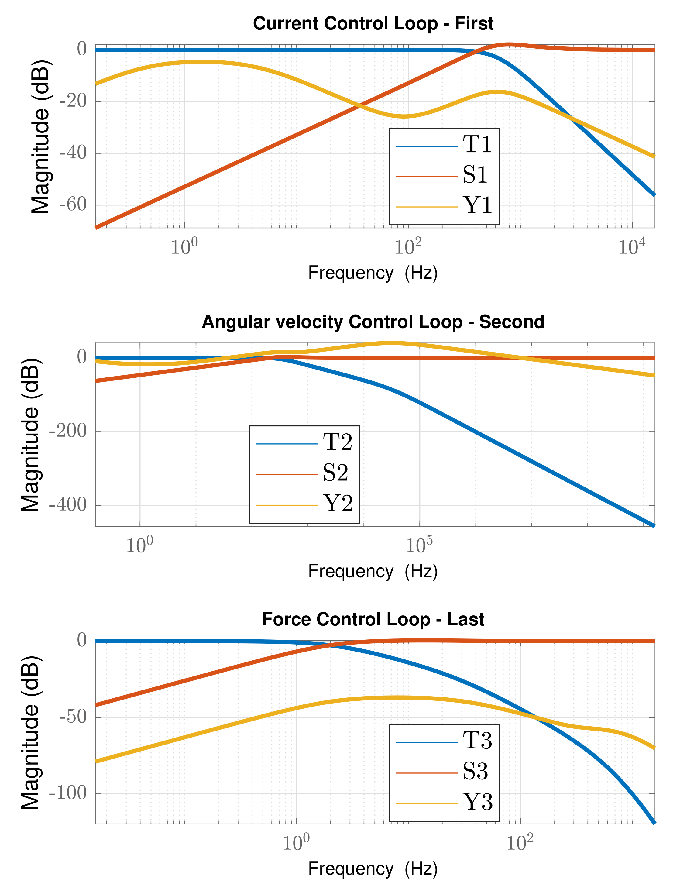
Youla parameterization is a robust control method that leverages closed-loop frequency shaping to attain the desired closed-loop behavior. These closed-loop transfer functions consist of ( T y ), known as a complementary sensitivity transfer function, sensitivity transfer function S y , and Youla Y transfer function (explained below). This method shapes closed-loop transfer functions while ensuring internal stability along with disturbance rejection at low frequencies and sensor noise and unmodeled disturbance rejections at high frequencies. This method was selected because of its ease of control design using the model-based approach for designing appropriate low-level controllers based on the developed bond graph models [36].
The central notion in this method is to form a closed-loop transfer function ( T y ) with a transfer function named Youla ( Y ( s ) ). Multiply Youla by the plant transfer function ( G p ) to create the desired closed-loop transfer function (Equation (11)). For good tracking performance in steady-state, the magnitude of T y ( s ) should be set to one at low frequencies. To ensure high-frequency noise rejection, T y ( s ) should be small at high frequencies:
T y ( s ) = Y ( s ) × G p ( s )
As a result, we can shape the closed-loop transfer function using Equation (11) (given we meet all the interpolation conditions for ensuring internal stability mentioned below). It should be noted that the Youla transfer function maps the desired reference signal to the actuator effort. With good target following, such as | T y ( s ) | = 1 at low frequency, the Youla transfer function is approximately equal to the inverse of the plant transfer function at low frequency and equal to the controller G c ( s ) transfer function at high frequency. Thus, keeping Youla’s magnitude small at high frequencies would reduce actuator effort and minimize the impact of sensor noise on the actuator.
The closed-loop transfer function ( T y ( s ) ) and the sensitivity transfer function ( S y ( s ) ) are complementary to each other, as shown by (Equation (12)). Due to this algebraic constraint, the sensitivity transfer function should be small at low frequencies (to reject low-frequency disturbances) and equal to one in magnitude at high frequencies:
S y ( s ) = 1 T y ( s )
If G p is stable, the feedback loop would be internally stable if and only if Y ( s ) is selected to be a stable transfer function. In this regard, Y y ( s ) , S y ( s ) , T y ( s ) , and G p × S y should all be stable to make the feedback loop internally stable. Consequently, to meet these conditions in case of an unstable pole ( α p ) which is repeated n-times in the plant ( G p ), Equations (13) and (14) define rational interpolation conditions, which must be met to enforce internal stability. If it is a single unstable pole (not repeated), Equation (13) is the only interpolation condition that needs to be satisfied:
T y ( α p ) = 1 , S y ( α p ) = 0
d k T y d s k ( α p ) = 0 , d k S y d s k ( α p ) = 0 , k 1 , n
If there is a repeated non-minimum phase zero ( α z ), zeros in the RHP (Right Half Plane), the interpolation conditions are met by Equations (15) and (16). If the unstable zero is only repeated once, Equation (15) is the only interpolation condition that must be satisfied [36]:
S ( α z ) = 1 , T ( α z ) = 0
d k S y d s k ( α z ) = 0 , d k T y d s k ( α z ) = 0 , k 1 , n
Once we ensure that the conditions in the Equations (13)–(16) are met, we can acquire the controller using Equation (17):
G c ( s ) = Y ( s ) × S y ( s ) 1

Cascaded Control

Since the brake-by-wire smart actuators are Single Input Multiple Output (SIMO) problems, we consider the cascaded control scheme. Cascaded control enables systems with relatively more nonlinearities to perform better and be more robust. Therefore, the controllers were designed using cascaded control to mitigate different nonlinearities in the brake actuators (e.g., mechanical friction, pressure nonlinearities). Each inner closed-loop is an open-loop for their outer loop controller design. The controller design of each plant is conducted through the Youla parameterization approach, as discussed in the previous section. Figure 3 shows this cascaded control design for EMB and EWB actuators. In the EMB and EWB, for the first loop, motor voltage is input, and motor current is the output. In the second loop, the motor’s desired current is input, and the motor’s angular velocity is output. Finally, for the outermost loop, the input is the desired motor angular velocity, and the clamping force is the output (the normal force of the brake pad on the wheel). The shaft’s current and angular velocity can be measured directly and is readily available, but the clamping force must be estimated or measured with a force sensor.
One important part of the EMB/EWB plant, which is not shown in Figure 3, is the current and voltage saturation. Current is saturated at ± 25 A, and voltage is set to saturate at ± 42 Volts. Because of these, the controllers might saturate and, therefore, make the plant unstable. A simple gain anti-windup was used to address the current saturation and to mitigate this issue (Figure 4). There could also be another anti-windup for the voltage saturation; however, normally, the voltage does not reach saturation levels if the current saturation has been addressed. Furthermore, adding an extra anti-windup may result in limiting the bandwidth of the closed-loop system. In addition, other anti-windup strategies such as the one in [37] or [38], which is specifically for cascaded controllers, could have been utilized.
In the EHB control design, a SISO controller was designed based on the linearized equations mentioned in Equations (5)–(7). The operating points taken for this linearization are u 0 = 0.3 and q c 0 = 0.3 × q 0 . q 0 is the steady-state value of q c y l . In addition, as mentioned before, it is assumed that u d = 1 u b . This continuous control law works well when building and dumping the pressure in the cylinder chamber. However, in the case of keeping constant pressure during the steady-state, we might run into the issue of having both build and dump valves open partially at the same time and therefore losing some of the master cylinder’s pressure which wastes energy. For example, u d = 0.7 and u b = 0.3 would hold the constant cylinder pressure, but this is not energy efficient as the pumps keep running. For this reason, a switching logic was added to the continuous Youla controller. This switching statement changes the values of u b and u d to zero once the clamping force error is within the desired threshold. Otherwise, it passes the same values from the controller to the plant as shown in Figure 5.

2.3. Optimization

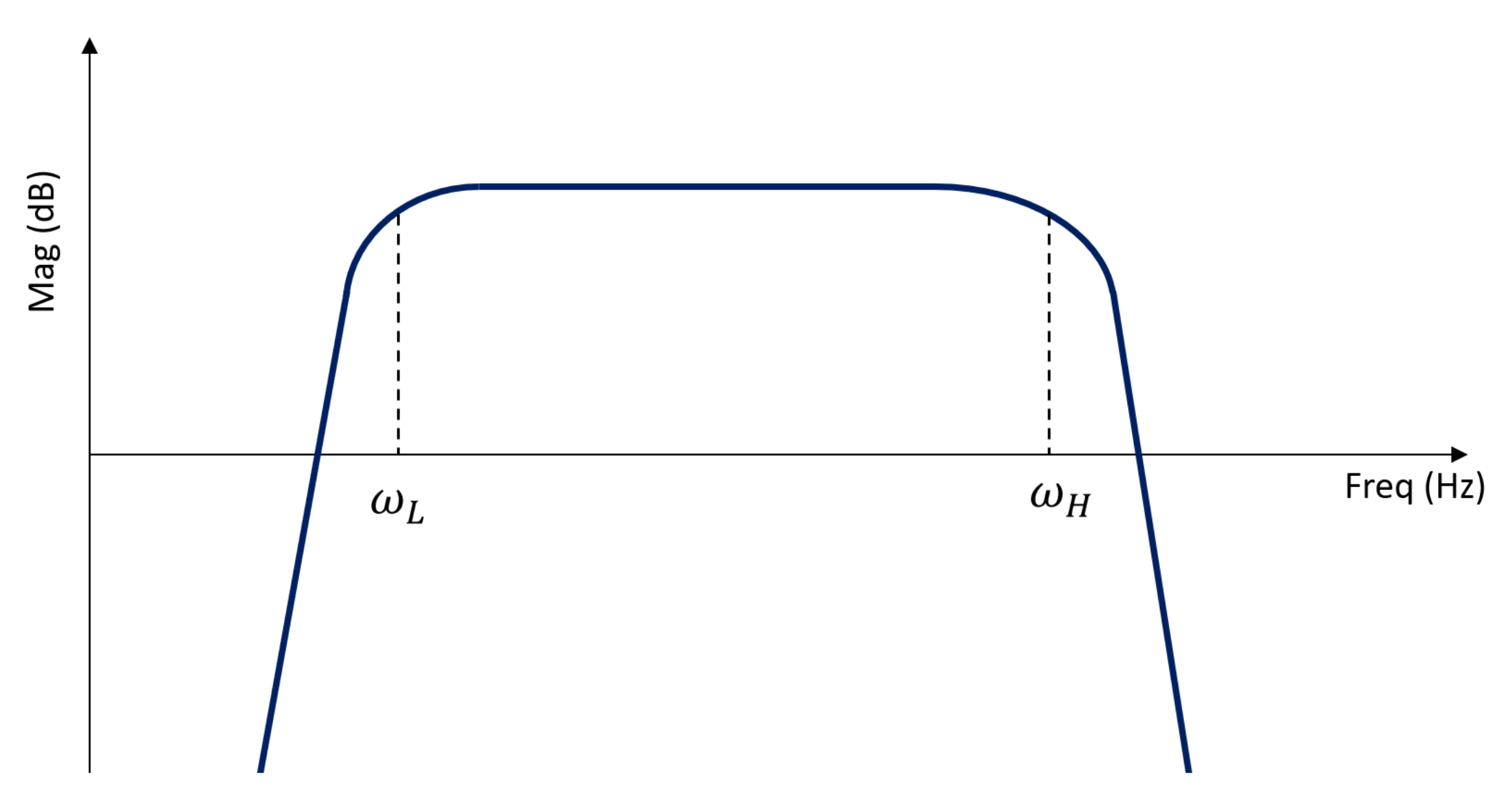
2.3.1. Linear Optimization: Using Transfer Functions

In this section, a multi-objective optimization scheme for brake-by-wire actuators based on their transfer functions is considered. This optimization considers dynamic responsiveness and the actuator’s effort as objective metrics.
After linearizing the plants, we can obtain their transfer functions. We then synthesize the controllers using the Youla parameterization technique discussed in Section 2.2. There are a few assumptions made when designing the controllers during the optimization process. Controllers are designed to create closed-loop transfer functions to be in a certain form. Equations (18), (19), (20), (21a), (21b), (22), (23a) and (23b) describe the form of Plant transfer function (Gp), Youla transfer function (Y), and closed-loop transfer function (T) for the first, second, and the third loop of EMB (EWB follows a similar control design pattern, and EHB follows the same pattern, but it only has one control loop, and therefore, the design choice is similar to the one in Equation (19)). The goal here is to design a closed-loop transfer function with the frequency shape of a second-order Butterworth filter and add extra first-order filters whenever necessary. For example, in Equation (21a), the second open-loop transfer function has an integrator that should not be canceled by the Youla transfer function. Hence, a high pass filter was added to the Youla transfer function ( 1 s + W 1 ). W 1 is the pole for the filter that is added to the Youla transfer function. This can be chosen in such a way that it does not affect the bandwidth of the closed-loop system. In this equation, G p 2 represents the plant transfer function of the second loop without the s in the numerator. Moreover, in the case of Equation (23a), a repeated first-order transfer function was added to the Youla transfer function to make this transfer function proper ( G p 3 is a fourth-order transfer function; for simplicity, we choose to use first-order poles. N-th order Butterworth filter could also be used in this case). More details on the design of these controllers are provided in [31]. It should be noted that ω n 1 , ω n 2 , and ω n 3 are chosen for each loop to have a specific bandwidth ( ω n 1 , ω n 2 , and ω n 3 are the Butterworth filter’s cut-off frequencies for the different added Butterworth filter to Youla transfer functions). In the case of EMB, this is 200 Hz, 10 Hz, and 2 Hz for the first, second, and last loop, respectively. For the EWB, they are chosen to be 500 Hz, 400 Hz, and 2 Hz. Finally, for EHB, it is chosen to be 2 Hz. Therefore, all of the brake-by-wire actuators have the same final closed-loop of 2 Hz for the clamp force loop. This is a deliberate choice to make sure all the brake-by-wire actuators have the same bandwidth (for the clamping force) for the final comparison in terms of energy and responsiveness metrics. The chosen control parameters mentioned here (such as ω n and ξ ) will remain the same over the course of all optimizations. This is performed to have fixed control design for the optimization procedure, and the only change will be the physical parameters of the system. Figure 6 shows the Bode magnitude plots of T, S, and Y for this type of control design.
G p I = J m s 2 + D m s + ( N s N p ) 2 K c a l ( L m J m ) × s 3 + ( R m J m + L m D m ) × s 2 + ( R m D m + L m ( N s N p ) 2 K c a l + K t 2 ) × s + R m ( N s N p ) 2 K c a l
Y 1 = 1 G p I × ω n 1 2 s 2 + 2 × ξ × ω n 1 × s + ω n 1 2 , T 1 = ω n 1 2 s 2 + 2 × ξ × ω n × s + ω n 1 2
G p 2 = T 1 × G p ω = ω n 1 2 s 2 + 2 × ξ × ω n × s + ω n 1 2 × K t × s J m s 2 + D m s + ( N s N p ) 2 K c a l
Y 2 = 1 G p 2 × ω n 2 2 s 2 + 2 × ξ × ω n 2 × s + ω n 2 2 × 1 s + W 1 × ( W 2 s + W 2 ) 2
T 2 = ω n 2 2 s 2 + 2 × ξ × ω n 2 × s + ω n 2 2 × s s + W 1 × ( W 2 s + W 2 ) 2
G p 3 = T 2 × G p F = ω n 2 2 s 2 + 2 × ξ × ω n 2 × s + ω n 2 2 × s s + W 1 × ( W 2 s + W 2 ) 2 × K c a l N s N p s
Y 3 = 1 G p 3 × ω n 3 2 s 2 + 2 × ξ × ω n 3 × s + ω n 3 2 × ( W 3 s + W 3 ) 4
T 3 = ω n 3 2 s 2 + 2 × ξ × ω n 3 × s + ω n 3 2 × ( W 3 s + W 3 ) 4
After designing the controllers, we then utilized the aforementioned transfer functions to optimize actuator response and actuator usage. The process of optimization starts with designing the controllers based on the physical parameters of the system and deriving these transfer functions as a function of the physical system parameters (since the parameters change, the G p s change, and therefore, these transfer functions will be different for each set of physical parameters).
The bandwidth of a plant is related to its dynamic response, and therefore, increasing the bandwidth would result in faster system response. The bandwidth of a system/plant is defined as the frequency range where the magnitude of the system gain does not drop below −3 dB. For EMB/EWB, the plant transfer function, which is chosen (denoted as G p here) for calculating the system bandwidth, is from voltage input to the clamping force output. For EHB, the plant transfer function maps u b to the clamping force. The bandwidth of the plant is denoted as B a n d w i d t h { G p } .
Another factor to consider is the actuator’s power usage which is related to the actuator’s effort, and hence, it is related to the Youla transfer function, denoted as Y ( s ) . The Youla transfer function for the overall system in case of cascaded control design would become Y s y s = Y 1 × Y 2 × Y 3 . In here, Y s y s stands for the Youla transfer function from the clamping force reference to the voltage input (or to the u b for the EHB), which is the Youla transfer function of the overall control system. It can be shown if the magnitude of T y ( s ) or the gain of closed-loop transfer function is one at low frequencies, the Youla transfer function at low frequencies is inversely related to the plant transfer function G p ( s ) (From Equation (11), if T y = 1 , then Y = 1 G p ). By increasing the plant gain at low frequency (approximately its DC gain, denoted as D C { G p } in this section), Y ( s ) will decrease at low frequencies.
Furthermore, we need to lower the overall values of the Youla transfer function magnitude at other important frequencies, especially around the plant bandwidth. This will ensure the reduction of the actuator effort in all possible frequencies. To this end, we can use an H2 norm of this transfer function. H2 norm is related to the output signal energy when the system input is an impulse [36]. Since we are interested in a specific frequency region of the Youla transfer function, a band-pass filter, see Figure 7, is used to emphasize the frequency region of interest. ω L and ω H are chosen to be 0.1 × B a n d w i d t h { G p } and 1 e 4 × B a n d w i d t h { G p } . This will ensure that the Youla transfer function magnitudes at low and mid-range frequencies stay low. The optimization problem is then formulated by combining all these costs as given in Equation (24):
minimize x & f ( x ) = α 1 × | | Y s y s × W Y | | 2 + α 2 × 1 D C { G p } + α 3 × 1 B a n d w i d t h { G p } subject to & x [ x m i n , x m a x ] ,
where α 1 , α 2 , and α 3 are tuning parameters, and x is the vector of physical parameters of the system that can be changed during the design process (e.g., gear ratios, moments of inertia, and motor’s inductance). x m i n and x m a x denote the minimum and maximum of the parameter set, respectively. W Y is the frequency weighting function for H 2 norm optimization. It should be noted that each cost in Equation (24) is normalized by its nominal value to ensure the minimization of the three costs is done without bias. A choice of physical parameters for each actuator, their initial and optimized value are given in Table 1.

2.3.2. Nonlinear Optimization

Using linear transfer functions to optimize the plants provide us with an optimized initial parameter set. Although this set might be good enough for primarily linear plants; most brake actuators are nonlinear due to different factors such as friction, plant saturation, and dead-zone. Therefore, to further optimize the plants, we should perform optimization with the nonlinear plants to consider all the nonlinear effects. Since all the plants are going to run in the feedback control environment in practice, the nonlinear optimization is done on the closed-loop systems. A 10 kN step clamp force reference target is chosen for the brake’s closed-loop system. The controllers are designed in the same way explained in the Section 2.2 and Section 2.3.1. The control parameters are fixed in the same way as the transfer function optimization while the physical parameters of the systems change. Since the physical parameters of the system are changed, we need to recalculate the controllers at each step of function evaluation in the optimization ( G p changes, and so does Y and G c ). Since the optimization is performed on nonlinear plants, a different objective function should be used. The objective function for the nonlinear optimization consists of four parts: energy usage, maximum power, settling time, and overshoot percentage. Energy usage ( E u s a g e ) is the total amount of energy used by the actuator to follow the target in two seconds (enough for the actuators to reach and hold the target). Maximum power ( max P u s a g e ) is the maximum power used by the actuator during the 2 s that the actuator follows the 10 kN step reference. Settling time ( T s ) is the time that it takes for the caliper force to build up to near ± 2 % of the steady-state value. Overshoot percentage ( O S % ) is the percentage that the maximum value of the caliper force deviates from the 10 kN reference target. Power usage for the EMB and EWB is defined as current multiplied by the voltage. For the EHB, we are adding up the amount of power loss (denoted as P b u i l d and P d u m p ) to be equal to the power usage (Figure 2a):
P b u i l d = e b u i l d × f b u i l d = ( P i n β h f V C y l × q c y l ) × { C d S b u b 2 ρ ( P in β h f V c y l q c y l ) }
P d u m p = e d u m p × f d u m p = ( β h f V C y l × q c y l ) × { C d S d u d 2 ρ ( β h f V c y l q c y l ) }
Taking all of these into account, the cost function for nonlinear optimization is given in Equation (Section 2.3.2). Note that each cost is normalized by its nominal value:
minimize x f ( x ) = α 1 × E u s a g e + α 2 × max P u s a g e + α 3 × T s + α 4 × O S % subject to x [ x m i n , x m a x ]

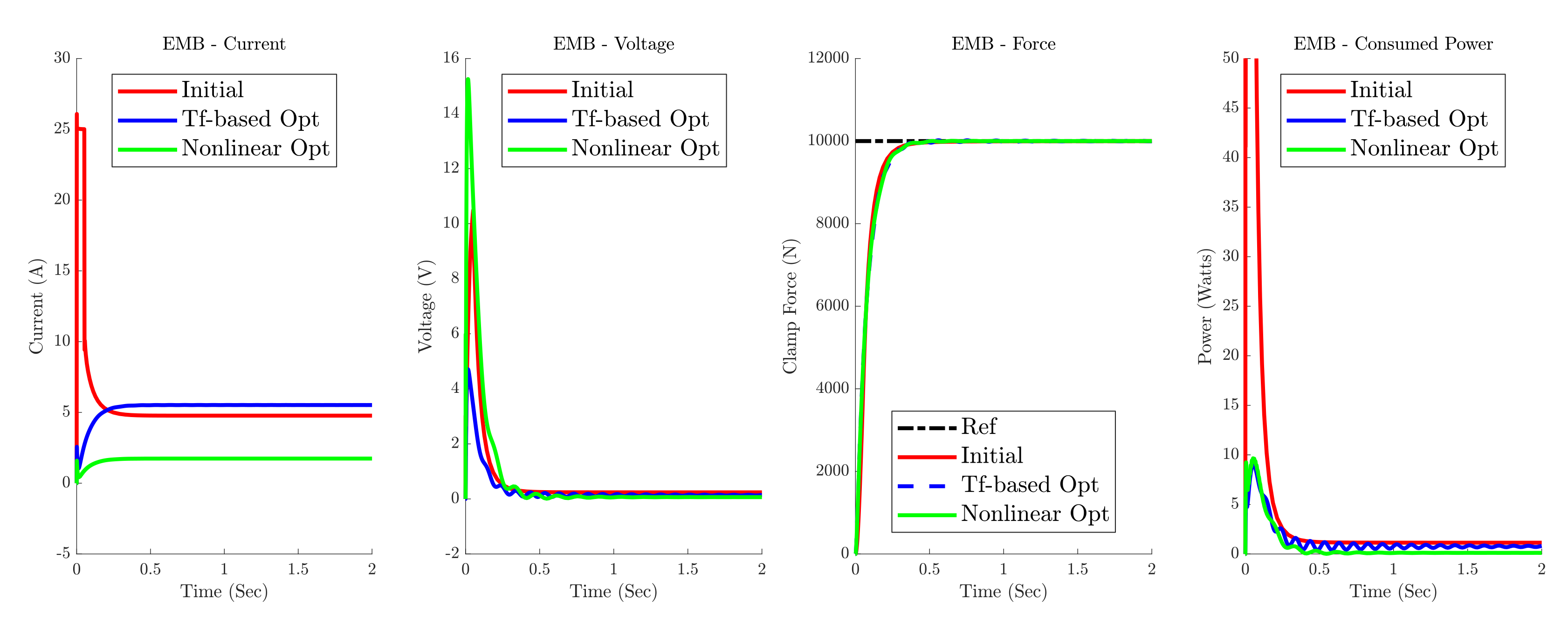
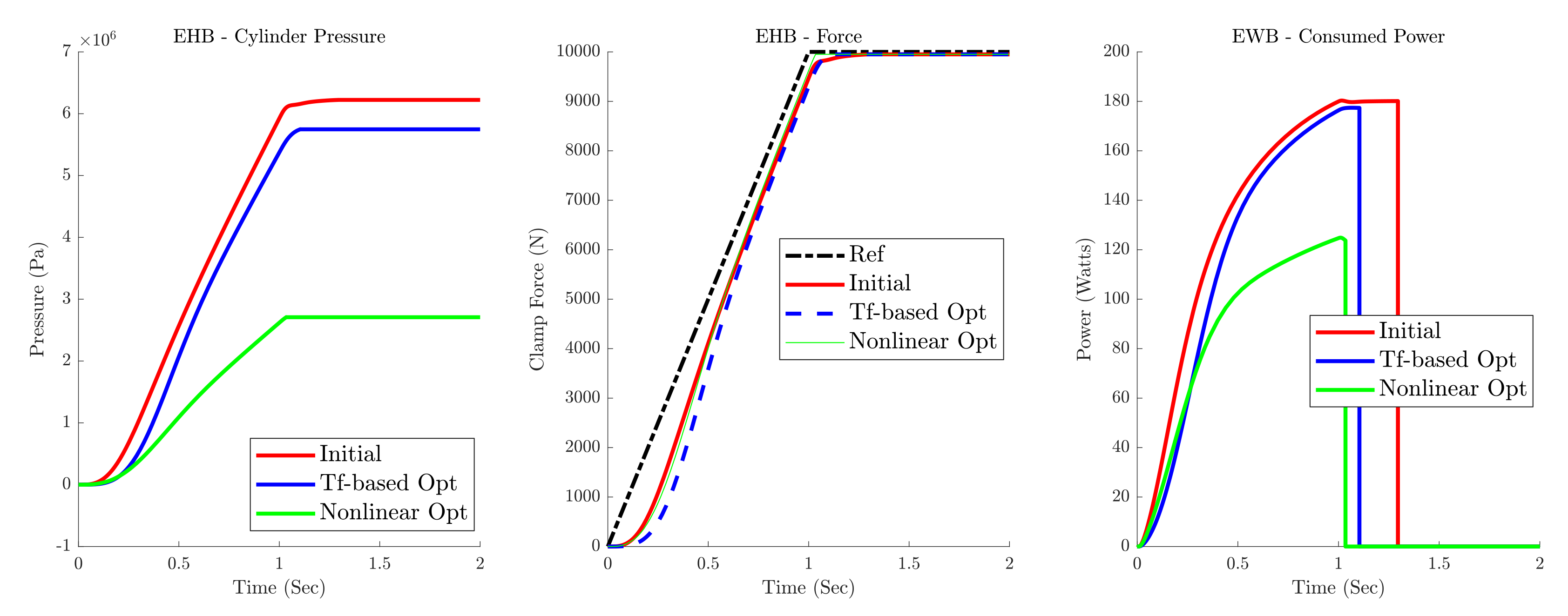
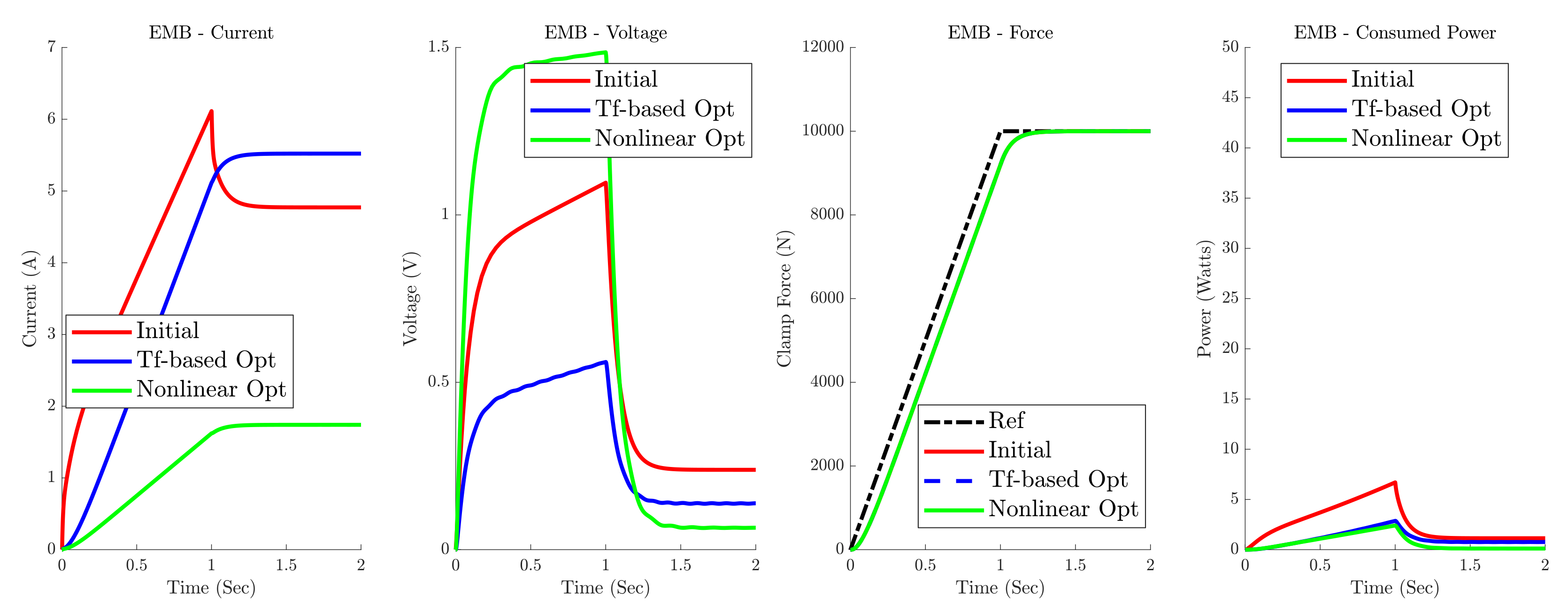
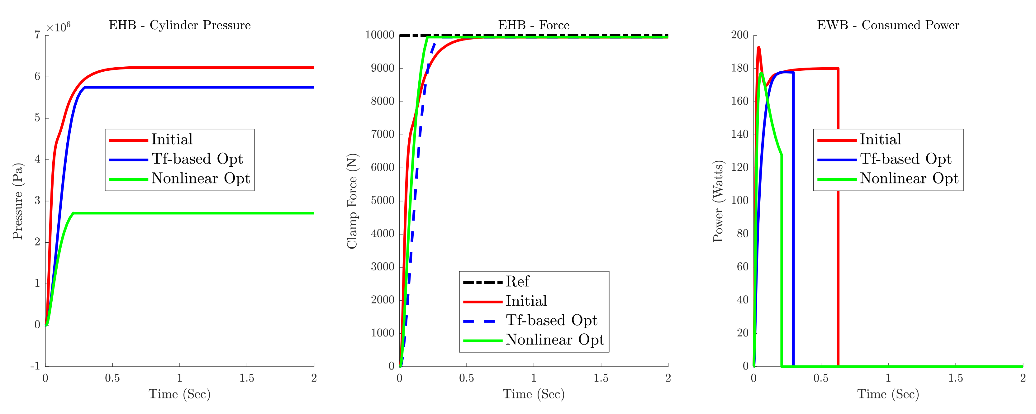
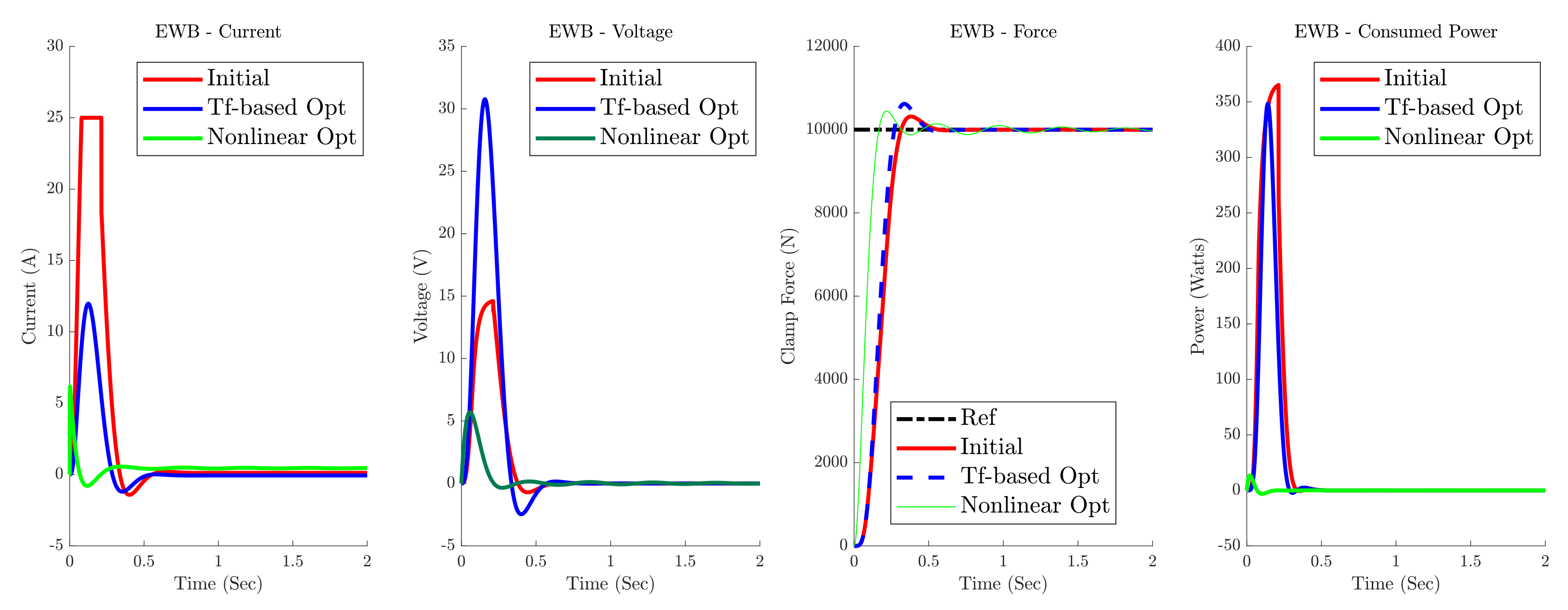
3. Results and Discussion

Figure 8, Figure 9 and Figure 10 show the results of a 10 k N clamp force step response and the linear and non-linear optimization of brake-by-wire actuators. These simulations are performed using the nonlinear plant of the actuators. The nonlinearities that exist in the EMB and EWB include motor current and voltage saturation, brake caliper saturation, and the Lugre friction model. The nonlinearities in the EHB include the valve nonlinearities and the dead-zone. The “Initial” represents the initial set of parameters of the plant before the optimization. The initial setting for each actuator is compared with a similar setting in the literature to make sure the results are sound and follow other researchers’ results. However, for the optimized plants’ results, since this is the first study that discusses optimization on these physical parameters, there are no other papers to compare the results with. The “TF-based Opt.” represents the linear transfer function optimization, and “Nonlinear Opt.” represents the results for the set of plant parameters after the optimization is performed using the nonlinear plants as discussed in Section 2.3.
For the EHB, Figure 8 shows that the transfer function-based and the nonlinear optimization both have reduced the cylinder pressure. It must be noted that the results for the initial set of parameters are consistent with [33]. The cylinder’s pressure in the Zhao et al. reaches steady-state around 0.3 s, similar to the results for this study. This shows that robust control along with the linearization is working for this EHB actuator. The readers have to note that the difference between the EHB model studied here is that the valves are considered to change continuously, and therefore, a continuous Youla control scheme is used to control the valves; however, in reality, this needs to be taken care of using a digital controller and pulse width modulation technique. The clamping force response time for the optimized simulation has also decreased from 0.5 s to around 0.3 s and 0.2 s for TF-based and nonlinear optimization, respectively. The power usage plot shows that, in all the cases, the power consumption stops once the actuators reach the steady-state target. This is because of the switching logic that closes both valves once they reach the steady-state value of the clamping force. Since the optimized plants reach the steady-state faster, and they use less actuation to do so, their energy and power usage is reduced (see Table 2).
For the EMB, Figure 9 illustrates that the clamping force step response is about the same for all plants. This is because the controllers are set to have the same bandwidth; they all have the same response. In this case, the nonlinearities are mitigated by robust controllers, and the current/voltage saturation is taken care of by the anti-windup compensator. As shown, the current reaches its saturation level for the initial EMB plant, and the gain anti-windup is shown to be working. However, the difference between the plants manifests itself in the power consumption plot. The initial plant uses a lot more power and energy to perform the same task as the optimized plants. Tf-based and nonlinear optimized plants both have a significantly smaller power usage, with the nonlinear optimized plant consuming a slightly lower amount of power. The overall energy consumption for these plants is summarized in Table 2. Comparing to Line et al., for the initial parameter setting, the clamping force also reaches the steady-state around 0.2 s [6]. The current is higher than the results shown in Line et al.; however, the voltage is not plotted for their results. One explanation is that a higher amount of current would result in lower voltage and vice versa.
For the EWB, Figure 10 shows the step response for all the plants. For the initial parameter setting, the clamping force reaches to steady-state in around 0.5 s. Compared to Che Hasan et al., which uses a PID controller, this is around 0.2 s faster [12]. Additionally, using the Youla parameterization along with cascaded control, the overshoot is also smaller. The voltage peak for both are around the same, although the voltage for this paper is slightly higher. The nonlinear optimized plant is showing a faster response than the transfer function optimized and the initial plant. The overshoot in the nonlinear optimization of the plant has also slightly decreased when compared with the Tf-based optimization plant. As shown, the current once again saturates for the initial plant. For this plant, the current was saturated for around 0.3 s, and the anti-windup compensation has taken care of this; however, this has negatively impacted the closed-loop response and made it slower. Looking at the power consumption, it is clear that the Tf-based opt. has used a slightly lower amount of power, and the nonlinear opt. has used a significantly lesser amount of actuation power. It should be noted that the voltage and current have undershot in all the plants, which comes from the fact that overshoots in the clamping force, as shown in Figure 10, are being compensated by these undershoots.
Similar to the step response, we have performed a ramp response of 10 kN/s with the saturation of 10 kN for the given plants. Figure 11, Figure 12 and Figure 13 show similar results to the ones of the step response as discussed previously. It should be noted that the ramp response is only discussed in this paper, and the cited papers above did not mention performing this test on the actuators.
Table 3 shows the amount of energy usage by each plant with a different set of parameters. Comparing the energy usage of brake-by-wire actuators in Table 2 and Table 3, we can conclude that EMB and EWB use significantly lower amounts of energy. However, looking once again at the Figure 8, Figure 9 and Figure 10, we can see that EHB has at least a 0.1–0.2 s faster response than the dry brake-by-wire actuators such as EMB and EWB.

4. Conclusions

In this paper, we presented the modeling and a new control strategy for three different brake-by-wire actuators. The physical optimization of these plants using linear transfer functions, and nonlinear plants were discussed, and the results were presented. The optimized results show a promising energy reduction when compared with the nominal parameters. EHB’s, EMB’s, and EWB’s energy consumption were reduced to around 10%, 3%, and 20% of their original sets of parameters, respectively. This method can be effectively utilized for other brake-by-wire actuators to reduce their energy consumption while increasing their dynamic response. It should be noted that in practice, other criteria such as structural, electrical, and heat transfer measures should be added to the optimization method. This can result in more constraints for the optimization problem, which in turn will alter the final results. However, the optimization framework and the objectives will stay the same. Usually, having more constraints will result in a lesser deviation from the initial results. However, as shown in the results, the gains in energy consumption and dynamic responsiveness are high enough to be considered even with added constraints to the optimization problem. This calls for more future studies.
This paper aims to create a framework for optimizing brake-by-wire actuators by considering the problem from the perspective of energy consumption and actuator dynamic response. This framework can be further expanded to add other measures such as cost, weight, and reliability.

Author Contributions

Conceptualization, E.A. and F.A.; methodology, E.A. and F.A.; software, E.A.; validation, E.A. and F.A.; formal analysis, E.A. and F.A.; supervision: F.A.; writing—original draft preparation, review and editing: E.A. and F.A.; funding acquisition: F.A. All authors have read and agreed to the published version of the manuscript.

Funding

This research received no external funding.

Institutional Review Board Statement

Not applicable.

Informed Consent Statement

Not applicable.

Data Availability Statement

Not applicable.

Conflicts of Interest

The authors declare no conflict of interest.

Abbreviations

The following abbreviations are used in this manuscript:
NotationDefinition
F c l Clamping force
q c y l Volumetric displacement of the cylinder fluid
p p Momentum of the caliper
x c a l Caliper displacement
P i n Pressure input
u b Duty ratio of the build valve
u d Duty ratio of the dump valve
C d Maximum flow coefficient of valve
S b Cross-sectional area of the build valve when fully open
S d Cross-sectional area of the dump valve when fully open
ρ Density of the brake fluid
β h f Bulk modulus of the brake fluid
V c y l Cylinder’s volume
S p Cylinder’s cross-section surface
b p Damping coefficient
m p Brake pad’s mass
x 0 Brake clearance
k c a l Caliper stiffness
I m Electric current
V i n Voltage input
ω m Angular velocity of the shaft
L m Inductance of the electric motor
R m Electrical resistance in the electric motor
K t Electromotive force constant
J m Total moment of inertia of the rotational parts
D m Axial viscous friction
N s Planetary gear reduction ratio
N p Ball-screw gear reduction ratio
NCombined gear reduction ( N s × N p )
q a x Shaft axial displacement
K a x Shaft axial stiffness
D a x Shaft axial viscous resistance
X w Wedge displacement
V w Wedge velocity
F m Motor force exerted to the wedge
α Wedge angle
μ c a l Friction coefficient between the pad and the wheel
τ f Lumped nonlinear frictions present in the actuator
σ 0 Contact (bristle) stiffness (Lugre friction model)
σ 1 Damping coefficient of the bristle (Lugre friction model)
σ 2 Viscous friction coefficient (Lugre friction model)
ω s Stribeck velocity (Lugre friction model)
jShape factor (Lugre friction model)
τ c Coulomb friction (Lugre friction model)
τ s Static friction (Lugre friction model)
T y ( s ) Complementary sensitivity transfer function
G p ( s ) Plant transfer function
S y ( s ) Sensitivity transfer function
Y ( s ) Youla transfer function
α p Unstable pole
α z Non-minimum phase zero
G c Controller transfer function
q c 0 The operating point of q c y l (for the purpose of linearization)
u 0 The operating point of u (for the purpose of linearization)
G p I Plant transfer function for the current loop ( I m V i n )
G p ω Plant transfer function for the omega loop ( ω I m )
G p F Plant transfer function for the Force loop ( F c l ω )
G p 2 Plant transfer function of the second loop without the s in the numerator
Y i Youla transfer function for the i-th loop
T i Closed-Loop transfer function of the i-th loop
W i Constants of the first order transfer functions added to Youla
ω n i Butterworth filters’ cut-off frequency
ξ Damping ratio of Butterworth filter
Y s y s Youla transfer function of the system ( Y 1 × Y 2 × Y 3 )
W Y Filter used to emphasize specific frequency region of Y s y s in the H2 norm
D C ( G p ) DC gain of plant tranfer function ( G p )
B a n d w i d t h { G p } Bandwidth of plant transfer function ( G p )
x m i n Minimum of the parameter set
x m a x Maximum of the parameter set
P b u i l d Amount of power loss in the build valve
P d u m p Amount of power loss in the dump valve
e b u i l d Effort in the build valve (refers to Figure 2a)
f b u i l d Flow in the build valve (refers to Figure 2a)
e d u m p Effort in the dump valve (refers to Figure 2a)
f d u m p Effort in the dump valve (refers to Figure 2a)
P u s a g e Power usage of the actuator
O S % Overshoot percentage
T s Settling time

References

  1. Lamnabhi-Lagarrigue, F.; Annaswamy, A.; Engell, S.; Isaksson, A.; Khargonekar, P.; Murray, R.M.; Nijmeijer, H.; Samad, T.; Tilbury, D.; Van den Hof, P. Systems & Control for the future of humanity, research agenda: Current and future roles, impact and grand challenges. Annu. Rev. Control 2017, 43, 1–64. [Google Scholar] [CrossRef]
  2. Yuan, Y.; Zhang, J.; Li, Y.; Lv, C. Regenerative Brake-by-Wire System Development and Hardware-In-Loop Test for Autonomous Electrified Vehicle. 2017. Available online: https://www.researchgate.net/publication/315859566_Regenerative_Brake-by-Wire_System_Development_and_Hardware-In-Loop_Test_for_Autonomous_Electrified_Vehicle (accessed on 7 January 2022). [CrossRef]
  3. Sinha, P. Architectural design and reliability analysis of a fail-operational brake-by-wire system from ISO 26262 perspectives. Reliab. Eng. Syst. Saf. 2011, 96, 1349–1359. [Google Scholar] [CrossRef]
  4. Gombert, B.D.; Schautt, M.; Roberts, R.P. The Development of alternative brake systems. In Encyclopedia of Automotive Engineering; Crolla, D., Foster, D.E., Kobayashi, T., Vaughan, N., Eds.; John Wiley & Sons, Ltd.: Chichester, UK, 2014; pp. 1–11. [Google Scholar] [CrossRef]
  5. Cheon, J.S. Brake by Wire System Configuration and Functions using Front EWB (Electric Wedge Brake) and Rear EMB (Electro-Mechanical Brake). Actuators 2010. [Google Scholar] [CrossRef]
  6. Line, C.; Manzie, C.; Good, M. Electromechanical Brake Modeling and Control: From PI to MPC. IEEE Trans. Control Syst. Technol. 2008, 16, 446–457. [Google Scholar] [CrossRef]
  7. Line, C.; Manzie, C.; Good, M. Robust control of an automotive electromechanical brake. IFAC Proc. Vol. 2007, 40, 579–586. [Google Scholar] [CrossRef]
  8. Sakamoto, T.; Hirukawa, K.; Ohmae, T. Cooperative control of full electric braking system with independently driven four wheels. In Proceedings of the 9th IEEE International Workshop on Advanced Motion Control, Istanbul, Turkey, 27–29 March 2006; pp. 602–606. [Google Scholar] [CrossRef]
  9. Hartmann, H.; Schautt, M.; Pascucci, A.; Gombert, B. eBrake®—The Mechatronic Wedge Brake. SAE Trans. 2002, 2146–2151. [Google Scholar] [CrossRef]
  10. Fox, J.; Roberts, R.; Baier-Welt, C.; Ho, L.M.; Lacraru, L.; Gombert, B. Modeling and Control of a Single Motor Electronic Wedge Brake. SAE Trans. 2007, 321–331. [Google Scholar] [CrossRef] [Green Version]
  11. Han, K.; Kim, M.; Huh, K. Modeling and control of an electronic wedge brake. Proc. Inst. Mech. Eng. Part C J. Mech. Eng. Sci. 2012, 226, 2440–2455. [Google Scholar] [CrossRef]
  12. Che Hasan, M.H.; Khair Hassan, M.; Ahmad, F.; Marhaban, M.H. Modelling and design of optimized electronic wedge brake. In Proceedings of the 2019 IEEE International Conference on Automatic Control and Intelligent Systems (I2CACIS), Selangor, Malaysia, 29 June 2019; pp. 189–193. [Google Scholar] [CrossRef]
  13. Cheon, J.S.; Kim, J.; Jeon, J. New Brake By Wire Concept with Mechanical Backup. SAE Int. J. Passeng. Cars Mech. Syst. 2012, 5, 1194–1198. [Google Scholar] [CrossRef]
  14. Emam, M.A.A.; Emam, A.S.; El-Demerdash, S.M.; Shaban, S.M.; Mahmoud, M.A. Performance of Automotive Self Reinforcement Brake System. J. Mech. Eng. 2012, 1, 7. [Google Scholar]
  15. Ahmad, F.; Hudha, K.; Mazlan, S.; Jamaluddin, H.; Aparow, V.; Yunos, M.M. Simulation and experimental investigation of vehicle braking system employing a fixed caliper based electronic wedge brake. Simulation 2018, 94, 327–340. [Google Scholar] [CrossRef]
  16. Ho, L.M.; Roberts, R.; Hartmann, H.; Gombert, B. The Electronic Wedge Brake—EWB; SAE International: Warrendale, PA, USA, 2006. [Google Scholar] [CrossRef]
  17. Putz, M.H. VE Mechatronic Brake: Development and Investigations of a Simple Electro Mechanical Brake; SAE International: Warrendale, PA, USA, 2010. [Google Scholar] [CrossRef]
  18. De Castro, R.; Todeschini, F.; Araújo, R.E.; Savaresi, S.M.; Corno, M.; Freitas, D. Adaptive-robust friction compensation in a hybrid brake-by-wire actuator. Proc. Inst. Mech. Eng. Part I J. Syst. Control Eng. 2014, 228, 769–786. [Google Scholar] [CrossRef]
  19. Gong, X.; Ge, W.; Yan, J.; Zhang, Y.; Gongye, X. Review on the Development, Control Method and Application Prospect of Brake-by-Wire Actuator. Actuators 2020, 9, 15. [Google Scholar] [CrossRef] [Green Version]
  20. Büchler, R. Future Brake Systems and Technologies-MK C1®-Continental’s brake system for future vehicle concepts. In 7th International Munich Chassis Symposium 2016; Pfeffer, P.D.P.E., Ed.; Springer Fachmedien Wiesbaden: Wiesbaden, Germany, 2017; pp. 717–723. [Google Scholar] [CrossRef]
  21. Shankar, R.; Marco, J.; Assadian, F. The Novel Application of Optimization and Charge Blended Energy Management Control for Component Downsizing within a Plug-in Hybrid Electric Vehicle. Energies 2012, 5, 4892–4923. [Google Scholar] [CrossRef]
  22. Yao, M.; Miao, J.; Cao, S.; Chen, S.; Chai, H. The Structure Design and Optimization of Electromagnetic-Mechanical Wedge Brake System. IEEE Access 2020, 8, 3996–4004. [Google Scholar] [CrossRef]
  23. Fengjiao, Z.; Minxiang, W. Multi-objective optimization of the control strategy of electric vehicle electro-hydraulic composite braking system with genetic algorithm. Adv. Mech. Eng. 2015, 7, 168781401456849. [Google Scholar] [CrossRef]
  24. Kwon, Y.; Kim, J.; Cheon, J.S.; Moon, H.; Chae, H.J. Multi-Objective Optimization and Robust Design of Brake By Wire System Components. SAE Int. J. Passeng. Cars Mech. Syst. 2013, 6, 1465–1475. [Google Scholar] [CrossRef]
  25. Hierlinger, T.; Dirndorfer, T.; Neuhauser, T. A method for the simulation-based parameter optimization of autonomous emergency braking systems. In Proceedings of the 25th International Technical Conference on the Enhanced Safety of Vehicles (ESV), Detroit, MI, USA, 5–8 June 2017; Available online: https://trid.trb.org/view/1483876 (accessed on 7 January 2022).
  26. Kelling, N.A.; Heck, W. The BRAKE Project—Centralized Versus Distributed Redundancy for Brake-by-WireSystems; SAE International: Warrendale, PA, USA, 2002. [Google Scholar] [CrossRef]
  27. Anwar, S. Anti-Lock Braking Control of a Hybrid Brake-by-Wire System. Proc. Inst. Mech. Eng. Part D: J. Automob. Eng. 2006, 220, 1101–1117. [Google Scholar] [CrossRef]
  28. Savaresi, S.M.; Tanelli, M. Active Braking Control Systems Design for Vehicles; Advances in Industrial Control; Springer: London, UK, 2010. [Google Scholar] [CrossRef]
  29. Khalil, H.K. Nonlinear control; Prentice Hall: Hoboken, NJ, USA, 2015. [Google Scholar]
  30. Soltani, A.; Assadian, F. New Slip Control System Considering Actuator Dynamics. SAE Int. J. Passeng. Cars Mech. Syst. 2015, 8, 512–520. [Google Scholar] [CrossRef] [Green Version]
  31. Arasteh, E.; Assadian, F. Advanced applications of hydrogen and engineering systems in the automotive industry. In New Robust Control Design of Brake-by-Wire Actuators; IntechOpen: London, UK, 2020. [Google Scholar] [CrossRef]
  32. Karnopp, D.; Margolis, D.L.; Rosenberg, R.C. System Dynamics: Modeling and Simulation of Mechatronic Systems, 5th ed.; Wiley: Hoboken, NJ, USA, 2012. [Google Scholar]
  33. Zhao, J.; Song, D.; Zhu, B.; Chen, Z.; Sun, Y. Nonlinear Backstepping Control of Electro-Hydraulic Brake System Based on Bond Graph Model. IEEE Access 2020, 8, 19100–19112. [Google Scholar] [CrossRef]
  34. Arasteh, E.; Assadian, F.; Filipozzi, L. Algorithm to Generate Target for Anti-Lock Braking System using Wheel Power. J. Mech. Aerosp. Eng. 2021, 2, 2–7. [Google Scholar]
  35. Wang, X.; Lin, S.; Wang, S. Dynamic Friction Parameter Identification Method with LuGre Model for Direct-Drive Rotary Torque Motor. Math. Probl. Eng. 2016, 2016, 1–8. [Google Scholar] [CrossRef] [Green Version]
  36. Assadian, F.; Mallon, K.R. Robust Control: Youla Parameterization Approach; John Wiley: Hoboken, NJ, USA, 2021. [Google Scholar]
  37. Zaccarian, L.; Teel, A.R. A common framework for anti-windup, bumpless transfer and reliable designs. Automatica 2002, 38, 1735–1744. [Google Scholar] [CrossRef]
  38. Todeschini, F.; Formentin, S.; Panzani, G.; Corno, M.; Savaresi, S.M.; Zaccarian, L. Nonlinear Pressure Control for BBW Systems via Dead-Zone and Antiwindup Compensation. IEEE Trans. Control Syst. Technol. 2016, 24, 1419–1431. [Google Scholar] [CrossRef]
Figure 1. Schematics of brake-by-wire actuators. (a) Electro-Hydraulic Brake [33]; (b) Electro-Mechanical Brake; (c) Electronic Wedge Brake [9].
Energies 15 00634 g001
Figure 2. Bond graphs of brake-by-wire actuators.
Energies 15 00634 g002
Figure 3. Cascaded control scheme for the EMB/EWB (a); The bottom Figure shows the decomposed system for control design (b).
Energies 15 00634 g003
Figure 4. Anti-windup gain used to compensate for the current saturation.
Energies 15 00634 g004
Figure 5. Control scheme for the EHB.
Energies 15 00634 g005
Figure 6. An example design of cascaded controllers for the EMB/EWB.
Energies 15 00634 g006
Figure 7. Band-pass filter, W Y , is used to emphasize specific frequency region of Youla transfer function in the H 2 norm optimization.
Energies 15 00634 g007
Figure 8. Comparison of the initial parameter sets vs. optimized in an EHB for a 10 kN step input. The clamp force plot for the initial parameter setting was consistent with Zhao et al. [33]. The optimized results are the novelty of this paper.
Energies 15 00634 g008
Figure 9. Comparison of the initial parameter sets vs. optimized in an EMB for a 10 kN step input. The clamp force plot for the initial parameter setting was consistent with Line et al. [6]. The optimized results are the novelty of this paper.
Energies 15 00634 g009
Figure 10. Comparison of the initial parameter sets vs. optimized in an EWB for a 10 kN step input. The clamp force plot for the initial parameter setting was consistent with Che Hassan et al. [12]. The optimized results are the novelty of this paper.
Energies 15 00634 g010
Figure 11. Comparison of the initial parameter sets vs. optimized in an EHB for a ramp input.
Energies 15 00634 g011
Figure 12. Comparison of the initial parameter sets vs. optimized in an EMB for a ramp input.
Energies 15 00634 g012
Figure 13. Comparison of the initial parameter sets vs. optimized in an EWB for a ramp input.
Energies 15 00634 g013
Table 1. Initial and optimized physical parameter values of EMB, EWB, and EHB and the range of the parameters.
ParameterUnitsLower BoundUpper BoundInitialTF-Based Opt.Nonlinear Opt.
L m H 4.48  × 10 5 × 10 3 5.6  × 10 5 6.36  × 10 5 2.8  × 10 3
R m Ω 2.50 × 10 2 × 10 1 × 10 2 2.5  × 10 2 3.76  × 10 2
J m k g m 2 s 2 6.0  × 10 5 5.8  × 10 4 2.9  × 10 4 7.19  × 10 5 1.03  × 10 4
D m N m s 2.0  × 10 4 1.5  × 10 2 × 10 3 2.02  × 10 4 9.0  × 10 4
EMB N s -7.96  × 10 5 1.3  × 10 3 6.37  × 10 4 1.3  × 10 3 1.2  × 10 3
N p -6/26618/2664.14  × 10 2 6.74  × 10 2 6.26  × 10 2
K c a l N m 1 2.3  × 10 7 4.3  × 10 7 3.35  × 10 7 4.3  × 10 7 4.19  × 10 7
K t N m A 1 5.0  × 10 2 5.2  × 10 1 6.97  × 10 2 1.59  × 10 1 4.3  × 10 1
L m H 4.48  × 10 5 × 10 3 5.6  × 10 5 4.7  × 10 3 4.48  × 10 5
R m Ω 2.50  × 10 2 × 10 1 × 10 2 2.5  × 10 2 2.6  × 10 2
J m k g m 2 s 2 6.0  × 10 5 5.8  × 10 4 2.9  × 10 4 5.8  × 10 4 9.26  × 10 5
D m N m s 2.0  × 10 4 1.5  × 10 2 × 10 3 2.0  × 10 4 2.1  × 10 4
EWB N s -7.96  × 10 5 7.96  × 10 4 4.77  × 10 4 7.96  × 10 4 7.89  × 10 4
N p -6/26618/2664.17  × 10 2 6.77  × 10 2 6.76  × 10 2
K c a l N m 1 2.3  × 10 7 4.3  × 10 7 3.35  × 10 7 4.3  × 10 7 4.29  × 10 7
K t N m A 1 5.0  × 10 2 5.2  × 10 1 6.97  × 10 2 5.0  × 10 2 5.88  × 10 2
α degrees1024.51024.524
m w k g 0.10.50.32.9  × 10 1 3.15  × 10 1
V c y l m 3 1.6  × 10 5 1.28  × 10 4 1.6  × 10 5 1.6  × 10 5 7.93  × 10 5
S b m 2 × 10 7 × 10 7 4.0  × 10 7 4.0  × 10 7 2.16  × 10 7
EHB S p m 2 6.38  × 10 4 1.02  × 10 2 1.6  × 10 3 1.7  × 10 3 3.7  × 10 3
m p k g × 10 1 21.9731.9671.25
K c a l N m 1 2.3  × 10 7 4.3  × 10 7 4.3  × 10 7 4.3  × 10 7 3.69  × 10 7
Table 2. Comparison of the amount of energy used in the 10 kN step response for 2 seconds (the amounts are in Joules).
EMBEWBEHB
Initial set15.560.13109.73
TF-Based optimized set2.731.9144.36
Nonlinear optimized set1.692.1429.70
Table 3. Comparison of the amount of energy used in the ramp response for 2 seconds (the amounts are in Joules).
EMBEWBEHB
Initial set5.1418.06174.42
TF-Based optimized set2.170.83128.67
Nonlinear optimized set1.410.8289.72
Publisher’s Note: MDPI stays neutral with regard to jurisdictional claims in published maps and institutional affiliations.

