Hydrodynamics of Moonpool-Type Floaters: A Theoretical and a CFD Formulation

Abstract

Moonpool-type floaters were initially proposed for applications such as artificial islands or as protecting barriers around a small area enabling work at the inner surface to be carried out in relatively calm water. In recent years, a growing interest on such structures has been noted, especially in relation to their use as heaving wave energy converters or as oscillating water column (OWC) devices for the extraction of energy from waves. Furthermore, in the offshore marine industry, several types of vessels are frequently constructed with moonpools. The present paper deals with the hydrodynamics of bottomless cylindrical bodies having vertical symmetry axis and floating in a water of finite depth. Two computation methods were implemented and compared: a theoretical approach solving analytically the corresponding diffraction problem around the moonpool floater and a computational fluid dynamics (CFD) solver, which considers the viscous effects near the sharp edges of the body (vortex shedding) as non-negligible. Two different moonpool-type configurations were examined, and some interesting phenomena were discussed concerning the viscous effects and irregularities caused by the resonance of the confined fluid.

1. Introduction

Moonpool-type floaters were initially proposed to be applied either as artificial islands or as structures enabling activities in their inner area, as they used their solid boundaries as protecting walls to the wave action. Nevertheless, in recent years, they have been associated with their use as wave energy converter (WEC) devices suitable for wave energy absorption, as well as floating pontoons for semi-submersible designs.

Several types of bottomless cylindrical hulls (known as moonpools) have been examined in the literature. The most common is a vertical cylinder with a vertical opening from the deck to keel through the hull [1], whereas square floaters with square moonpools have been also studied [2,3]. Additional types concern toroidal configurations consisting of a circular (core) section centered upon a large circle (ring) with an infinitesimally small [4] and finite [5] slenderness core-to-ring-radius ratio, as well as two coaxial surface piercing truncated circular cylinders [6]. The latter geometry was encompassed by an exterior partially immersed toroidal structure of finite volume and an interior coaxial free surface-piercing truncated cylinder. Thus, an internal annular free surface was developed, which was totally enclosed between the solid boundaries of the cylinders and open to the exterior fluid domain beneath the concentric bodies.

Hydrodynamics of the isolated truncated hollow cylindrical bodies have been investigated in the past. Garrett [7] presented an analytical solution of the wave scattering problem by a vertical bottomless partially immersed circular cylinder with infinitesimal wall thickness using matched axisymmetric eigenfunction expansions. Analytical computations of the exciting wave forces and moments on the hollow cylindrical shell structure, together with sway and pitch hydrodynamic coefficients, were derived by Miloh [8]. He also derived analytic expressions for the amplification ratios of heave (pumping) and pitch (seiche) modes of water motions inside the pond. The corresponding hydrodynamic characteristics of an open-ended vertically floating circular cylinder, as well as the induced water motion in the interior basin, accounting for the effect of the finite wall thickness, were presented by [1,9]. Furthermore, Liu et al. [10] investigated the second-order sum frequency wave loads on a hollow cylindrical shell structure in long crested irregular seas. Additionally, in [11,12] the solutions of the diffraction and radiation problems of a moonpool cylindrical body of infinite thickness and of a partially bottom-opened moonpool were presented. A moonpool with a restricted entrance was also studied. In [13], it was shown that the motion of the water inside the body was amplified as the size of the moonpool entrance was reduced. In addition, Liu et al. [14] measured the viscous effect of a moonpool cylindrical structure with a restricted entrance by introducing a quadratic dissipation assuming an additional dissipative disk at the moonpool entrance.

Regarding the two coaxial surface piercing truncated circular cylinder configuration, the solutions of the linearized diffraction and radiation problems around two independently moving concentric truncated cylinders were presented in [6,15]. Furthermore, the mean- and the time-dependent second-order wave loads on such a type of floating structures were evaluated in [16,17]. Recently, Chao and Kim [18] investigated the hydrodynamic performance of a two-body WEC by applying analytical solutions, whereas Kong et al. [19] examined a moonpool platform-wave energy buoy composed of an inner cylindrical buoy and an outer toroidal-cylinder for wave power extraction by the relative heave motions between the inner and outer buoys.

Apart from wave energy applications, concentric surface-piecing circular cylindrical bodies have also been investigated, combined with the trapped wave modes that they can develop, i.e., the localized oscillations of the enclosed formed free surface area, whereas the motion in the exterior fluid region decayed to zero. Abramson [20] presented a comprehensive review of liquid sloshing problems in moving containers, while Shipway and Evans [21] examined the wave trapping phenomena by two concentric circular cylindrical shells with a vertical axis and a zero thickness. As an extension of [21]’s work, McIver and Newman [22] studied the case of vertically axisymmetric trapping structures, of finite volumes, composed by two concentric interior free surfaces.

All the aforementioned research is based on potential flow methodologies concerning the hydrodynamic solutions of several types of bottomless cylindrical hulls. Nevertheless, over the last decade, there has been a significant interest in computational fluid dynamics (CFD) modelling due to its detailed results. CFD modelling solves the fluid flow problem using Navier–Stokes equations, where the hydrodynamics of random-shape floating structures can be calculated in detail, providing representative results of the flow physics. Several authors have studied the importance of including viscosity in moonpool problems using CFD modelling. Lu et al. [23] investigated the possibility of finding an artificial, empirically-based damping coefficient to the free surface condition inside a moonpool device applied to potential flow models. The latter exhibit overestimated magnitudes of wave forces as the fluid resonance takes place; hence, by introducing an artificial damping term, the potential flow model may work as well as the viscous fluid model. Lu et al. [24] extended the results from [23] on the wave elevation inside a moonpool body; whereas, in [25,26], the piston-mode in a 2D moonpool under forced heave oscillations was evaluated using a linear potential solver coupled to a viscous Navier–Stokes modelling. In addition, Fredriksen et al. [27] investigated, numerically and experimentally, how a low forward/incoming current speed influences the resonant piston-mode resonance in a moonpool. They concluded that the moonpool behavior was marginally reduced with a low forward velocity, whereas this reduction was dependent on the heave forcing amplitude. Recently, in [28] a viscous damping model for energy losses of a 2D fluid response in a moonpool due to wall friction and flow separation was proposed. Furthermore, the limitations of boundary element method solvers when viscous effects near floater’s sharp edges were taken into account and were exploited in [29] in the case of a moonpool type floater.

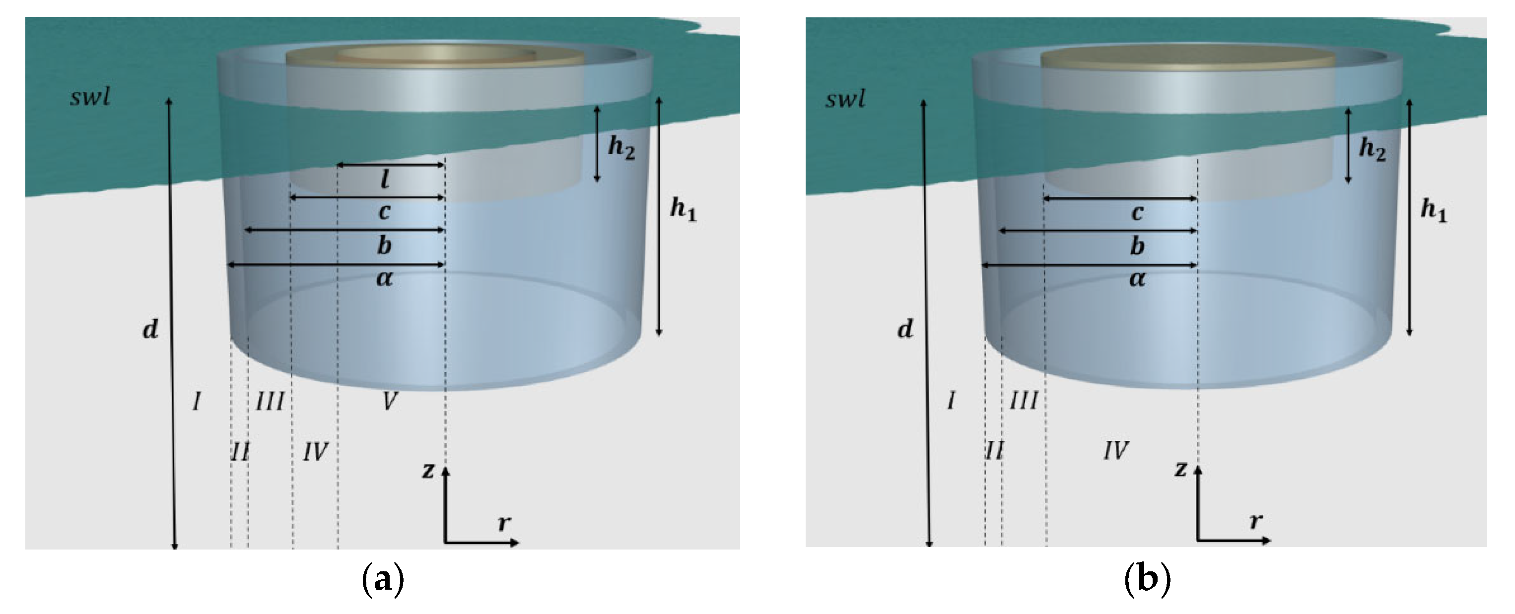
In the present article, two different geometric configurations of a moonpool-type floater were investigated; a floater encompassed by two coaxial, free-surface piercing toroidal cylinders with vertical symmetry axes (Configuration 1, see Figure 1a) and a floater consisting of an external toroidal cylinder and an internal coaxial surface piercing truncated circular cylinder (Configuration 2, see Figure 1b). In the annular and the cylindrical fluid areas formed between the cylinders’ vertical walls, oscillations of the enclosed water columns were developed. A semi-analytical model was used to solve the wave diffraction problem in the context of linear potential theory [30]. The method of matched axisymmetric eigenfunction expansions was applied to solve the relevant hydrodynamic problem, according to which the flow field around and inside the examined body was subdivided in coaxial ring-shaped fluid regions. Hence, appropriate series representations of the velocity potential can be established in each region, which were matched at the boundaries of adjacent fluid domains by enforcing the continuity conditions of the hydrodynamic pressure and the radial velocity in order to determine the unknown coefficients in the expressions of the diffraction potential. The exciting wave forces/moments and the wave elevation on both case studies were calculated and compared focusing on the resonant wave frequencies. Furthermore, the accuracy of the semi-analytical formulation was assessed in comparison to high fidelity CFD simulations.

The present work is structured as follows: in Section 2 the solution of the diffraction problem is formulated, along with the evaluation of the hydrodynamic forces and wave elevation around/inside the examined case studies. Section 3 is dedicated to the presentation of the used CFD solver, whereas, in Section 4, the outcomes of the two methods (i.e., semi-analytical and CFD solvers) are compared for the two moonpool arrangements. Finally, conclusions are drawn in Section 5.

2. Material and Methods

2.1. Velocity Potential Representation

Two coaxial, free-surface piercing toroidal cylinders with vertical symmetry axes are considered floating in constant water depth d. The cylinders are exposed to the action of a regular wave-train of wave frequency $\omega$ and amplitude $H/2$. The draughts of the moonpool bodies are denoted by $h_1$ and $h_2$, respectively. Cylindrical co-ordinates $\left(r,\theta ,z\right)$ are introduced with the $z$ axis positive upwards and with origin on the seabed (see Figure 1). In the present formulation, viscous effects were neglected, whereas the fluid was assumed incompressible. Furthermore, the fluid’s motions were assumed to be small, so that the linearized diffracted problem could be considered.

The fluid flow is described by the velocity potential expressed as:

$$\Phi \left(r,\theta ,z;t\right)=Re\left[\mathsf{\phi }\left(r,\theta ,z\right)e^{-i\omega t}\right]$$

(1)

with

$$\mathsf{\phi }\left(r,\theta ,z\right)={\mathsf{\phi }}_D\left(r,\theta ,z\right)={\mathsf{\phi }}_0\left(r,\theta ,z\right)+{\mathsf{\phi }}_7\left(r,\theta ,z\right)$$

(2)

Here, ${\mathsf{\phi }}_0$ is the velocity potential of the undisturbed incident harmonic wave and ${\mathsf{\phi }}_7$ is the diffraction potential for the restrained body in the wave impact. The diffraction potential is described by the velocity potential ${\mathsf{\phi }}_D$.

The undisturbed velocity potential of an incident wave train propagating along the positive axis can be expressed in cylindrical coordinates as:

$${\mathsf{\phi }}_0\left(r,\theta ,z\right)=-i\omega \frac{H}{2}\frac{Z_0\left(z\right)}{Z_0^{’}\left(d\right)}{\displaystyle \sum }_{m=0}^{\infty }{\epsilon }_m{i}^m{J}_m\left(kr\right)\cos \left(m\theta \right)$$

(3)

In Equation (3) $J_m$ stands for the mth order Bessel function of first kind, ${\epsilon }_m$ is the Neumann’s symbol, i.e., ${\epsilon }_0=1,{\epsilon }_m=2$ for $m\ge 1$, and $Z_0$ is derived by:

$$Z_0\left(z\right)={\left[\frac{1}{2}\left[1+\frac{\sin \mathrm{h}\left(2kd\right)}{2kd}\right]\right]}^{-\frac{1}{2}}\cos h\left(kz\right)$$

(4)

with $Z_0^{\prime }\left(d\right)$ being its derivative at z = d. The wave number k and the wave frequency $\omega$ are related by the dispersion equation i.e.,: ${\omega }^2=kg\tan \mathrm{h}\left(kd\right)$.

In accordance with Equation (3) the total diffracted potential of the flow field around the examined moonpool can be written in the form:

$${\mathsf{\phi }}_D\left(r,\theta ,z\right)=-i\omega \frac{H}{2}{\displaystyle \sum }_{m=0}^{\infty }{\epsilon }_m{i}^m{\mathsf{\Psi }}_{D,m}\left(r,z\right)\cos \left(m\theta \right)$$

(5)

The ${\mathsf{\Psi }}_{D,m}$ denote the principal unknowns of the problem. The subscript D stands for the diffraction problem, whereas the subscript m indicates the modes that should be taken into consideration within the solution of the corresponding problem.

The potential ${\mathsf{\phi }}_D$ must satisfy:

$$\Delta {\mathsf{\phi }}_D=\frac{{\partial }^2{\mathsf{\phi }}_D}{\partial r^2}+\frac{1}{r}\frac{\partial {\mathsf{\phi }}_D}{\partial r}+\frac{1}{r^2}\frac{{\partial }^2{\mathsf{\phi }}_D}{\partial {\theta }^2}+\frac{{\partial }^2{\mathsf{\phi }}_D}{\partial z^2}=0$$

(6)

with the linearized boundary conditions:

on the free surface z = d:

$${\omega }^2{\mathsf{\phi }}_D-g\frac{\partial {\mathsf{\phi }}_D}{\partial z}=0$$

(7)

on the seabed z = 0:

$$\frac{\partial {\mathsf{\phi }}_D}{\partial z}=0$$

(8)

on the body’s bottom ($z=d-h_1$, $b\le r\le a$ and $z=d-h_2,l\le r\le c$):

$$\frac{\partial {\mathsf{\phi }}_D}{\partial z}=0$$

(9)

on the body’s side walls ($d-h_1\le z\le d$, $r=a,b\mathrm{and}d-h_2\le z\le d,r=c,l$):

$$\frac{\partial {\mathsf{\phi }}_D}{\partial r}=0$$

(10)

It is also required that the scattered potential satisfies an appropriate radiation condition as $r\to \infty$ which has the form [1,31]:

$$\underset{r\to \infty }{\lim }\sqrt{r}\left(\frac{\partial }{\partial r}-ik\right){\mathsf{\phi }}_7=0$$

(11)

In addition, both the velocity potential and its derivatives $\frac{\partial {\mathsf{\phi }}_D}{\partial r}$ must be continuous at the boundaries $r=a,b,c,l$ of the neighboring ring elements shown in Figure 1a. This results in: for $0<z<d-h_1$, and $r=a$:

$$\begin{array}{c}{\Psi }_{D,m}^I\left(a,z\right)={\Psi }_{D,m}^{II}\left(a,z\right)\end{array}$$

(12)

$$\begin{array}{c}{\frac{\partial {\Psi }_{D,m}^I\left(r,z\right)}{\partial r}|}_{r=a}={\frac{\partial {\Psi }_{D,m}^{II}\left(r,z\right)}{\partial \mathit{r}}|}_{r=a}\end{array}$$

(13)

for $0<z<d-h_1$, and $r=b$:

$$\begin{array}{c}{\Psi }_{D,m}^{II}\left(b,z\right)={\Psi }_{D,m}^{III}\left(b,z\right)\end{array}$$

(14)

$$\begin{array}{c}{\frac{\partial {\Psi }_{D,m}^{II}\left(r,z\right)}{\partial r}|}_{r=b}={\frac{\partial {\Psi }_{D,m}^{III}\left(rz\right)}{\partial r}|}_{r=b}\end{array}$$

(15)

for $0<z<d-h_2$, and $r=c$:

$$\begin{array}{c}{\Psi }_{D,m}^{III}\left(c,z\right)={\Psi }_{D,m}^{IV}\left(c,z\right)\end{array}$$

(16)

$$\begin{array}{c}{\frac{\partial {\Psi }_{D,m}^{III}\left(r,z\right)}{\partial r}|}_{r=c}={\frac{\partial {\Psi }_{D,m}^{IV}\left(r,z\right)}{\partial r}|}_{r=c}\end{array}$$

(17)

for $0<z<d-h_2$, and $r=l$:

$$\begin{array}{c}{\Psi }_{D,m}^{III}\left(c,z\right)={\Psi }_{D,m}^{IV}\left(\mathbf{c},z\right)\end{array}$$

(18)

$$\begin{array}{c}{\frac{\partial {\Psi }_{D,m}^{III}\left(r,z\right)}{\partial r}|}_{r=c}={\frac{\partial {\Psi }_{D,m}^{IV}\left(r,z\right)}{\partial r}|}_{r=c}\end{array}$$

(19)

The superscripts I, II, III, IV, V imply quantities corresponding to respective types of ring elements.

The procedure for the determination of the velocity potential around a moonpool body that is exposed to the action of surface gravity waves has been presented thoroughly in previous studies: [1,5,6,9,15], to name a few. This procedure is extended here to the case of two coaxial surface piercing toroidal vertical cylinders. The following equations present proper series representations of the functions ${\mathsf{\Psi }}_{D,m}^i,i=I,II,III,IV,V$ in each fluid region around the body:

(a)

Infinite fluid domain, Type I ($a\le r,0\le z\le d$):

$$\frac{1}{d}{\Psi }_{D,m}^I=\left\{J_m\left(kr\right)-\frac{J_m\left(ka\right)}{H_m\left(ka\right)}{H}_m\left(kr\right)\right\}\frac{Z_0\left(z\right)}{d{Z}_0^{\prime }\left(d\right)}+{\displaystyle \sum }_{j=0}^{\infty }{F}_{mj}^I\frac{K_m\left(a_{j}r\right)}{K_m\left(a_{j}a\right)}{Z}_j\left(z\right)$$

(20)

where $H_m,K_m$ is the m-th order Hankel function of the first kind and the modified Bessel function of the second type, respectively. In addition, $Z_j\left(z\right)$ are orthonormal functions in $\left[0,d\right]$ defined by Equation (4) for $j=0$ and for j > 0:

$$Z_j\left(z\right)={\left[\frac{1}{2}\left[1+\frac{\sin \left(2a_{j}d\right)}{2a_{j}d}\right]\right]}^{-\frac{1}{2}}\cos \left(a_{j}z\right),j>0$$

(21)

The terms $a_j$ are the roots of the transcendental equation: ${\omega }^2+a_{j}g\tan \left(a_{j}d\right)=0$, which proposes one imaginary $a_0=-ik,k>0$ and infinite number of real roots.

(b)

Second fluid domain, Type II ($b\le r\le a,0\le z\le d-h_1$):

$$\frac{1}{d}{\Psi }_{D,m}^{II}={\displaystyle \sum }_{n=0}^{\infty }{\epsilon }_n\left[R_{mn}^{II}\left(r\right)F_{mn}^{II}+R_{mn}^{*II}\left(r\right)F_{mn}^{*II}\right]\cos \left(\frac{n\pi z}{d-h_1}\right)$$

(22)

where ${\epsilon }_n$ stands for the Neumann’s symbol and the functions $R_{mn}^{II}\left(r\right),R_{mn}^{*II}\left(r\right)$ are presented in Appendix A.

(c)

Third fluid domain, Type III ($c\le r\le b,0\le z\le d$):

$$\frac{1}{d}{\Psi }_{D,m}^{III}={\displaystyle \sum }_{i=0}^{\infty }\left[R_{mi}^{III}\left(r\right)F_{mi}^{III}+R_{mi}^{*III}\left(r\right)F_{mi}^{*III}\right]Z_i\left(z\right)$$

(23)

where $Z_i$ are orthonormal functions in $\left[0,d\right]$ defined by Equations (4) and (21) for $i=0,i>0$, respectively. The functions $R_{mi}^{III}\left(r\right),R_{mi}^{*III}\left(r\right)$ are presented in Appendix A.

(d)

Fourth fluid domain, Type IV ($l\le r\le c,0\le z\le d-h_2$):

$$\frac{1}{d}{\Psi }_{D,m}^{IV}={\displaystyle \sum }_{s=0}^{\infty }{\epsilon }_s\left[R_{ms}^{IV}\left(r\right)F_{ms}^{IV}+R_{ms}^{*IV}\left(r\right)F_{ms}^{*IV}\right]\cos \left(\frac{s\pi z}{d-h_2}\right)$$

(24)

Here ${\epsilon }_s$ stands for the Neumann’s symbol and the functions $R_{ms}^{IV}\left(r\right),R_{ms}^{*IV}\left(r\right)$ are defined in Appendix A.

(e)

Fifth fluid domain, Type V ($0\le r\le l,0\le z\le d$):

$$\frac{1}{d}{\Psi }_{D,m}^V={\displaystyle \sum }_{q=0}^{\infty }{F}_{mq}^V\frac{I_m\left(a_{q}r\right)}{I_m\left(a_{q}l\right)}{Z}_q\left(z\right)$$

(25)

where $Z_q$ are orthonormal functions in $\left[0,d\right]$ defined by Equations (4) and (21) for $q=0,q>0$, respectively, whereas the term $I_m$ is the mth order modified Bessel function of the first kind. We note that the modified Bessel function of second type $K_m\left(a_{q}r\right)$ does not appear in the velocity potential representation of this fluid domain type, as the function $K_m$ has a singular behavior at $r\to 0$. The latter has namely a contribution proportional to ${(l/r)}^m$ for $m\ne 0$ and $\log \left(r\right)$ for $m=0$ at $r\to 0$ [32].

Based on the derived velocity potentials in each fluid domain, the continuity requirements of the hydrodynamic pressure and radial velocity at the boundaries of neighboring fluid regions, expressed through Equations (12)–(19), along with the kinematic boundary conditions at the vertical walls of the body, are then to be fulfilled (see Equation (10)). Hence, the linear system of equations for the determination of the unknown Fourier coefficients $F_{mj}^l,l=I,II,III,IV,V$, and $F_{mj}^{*s},s=II,III,IV,$ in each fluid domain, was derived. The solution procedure is presented in the following Section 2.2.

2.2. Solution Procedure

In this subsection, the solution procedure for determining the unknown Fourier coefficients in each fluid domain is presented. Towards this goal, we first expressed the velocity potentials of the fluid domains at their vertical boundaries. To this end, by accounting for the values of the functions $R_{mn}^{II}\left(r\right),R_{mn}^{*II}\left(r\right),R_{mi}^{III}\left(r\right),R_{mi}^{*III}\left(r\right),R_{ms}^{IV}\left(r\right),R_{ms}^{*IV}\left(r\right)$ (see Appendix A) at $r=a,b,c\mathrm{and}r=l,$ the potential functions ${\mathsf{\Psi }}_{D,m}^i,i=I,II,III,IV,V$, see Equations (20), (22)–(25), can be reduced to the following simple series expressions at $r=a,b,c,l$:

$$\frac{1}{d}{\mathsf{\Psi }}_{D,m}^I\left(a,z\right)={\displaystyle \sum }_{j=0}^{\infty }{F}_{mj}^I{Z}_j\left(z\right)$$

(26)

$$\frac{1}{d}{\mathsf{\Psi }}_{D,m}^{II}\left(a,z\right)={\displaystyle \sum }_{n=0}^{\infty }{\epsilon }_n{F}_{mn}^{II}\cos \left(\frac{n\pi z}{d-h_1}\right)$$

(27)

$$\frac{1}{d}{\mathsf{\Psi }}_{D,m}^{II}\left(b,z\right)={\displaystyle \sum }_{n=0}^{\infty }{\epsilon }_n{F}_{mn}^{*II}\cos \left(\frac{n\pi z}{d-h_1}\right)$$

(28)

$$\frac{1}{d}{\mathsf{\Psi }}_{D,m}^{III}\left(b,z\right)={\displaystyle \sum }_{i=0}^{\infty }{F}_{mi}^{III}{Z}_i\left(z\right)$$

(29)

$$\frac{1}{d}{\mathsf{\Psi }}_{D,m}^{III}\left(c,z\right)={\displaystyle \sum }_{i=0}^{\infty }{F}_{mi}^{*III}{Z}_i\left(z\right)$$

(30)

$$\frac{1}{d}{\mathsf{\Psi }}_{D,m}^{IV}\left(c,z\right)={\displaystyle \sum }_{s=0}^{\infty }{\epsilon }_s{F}_{ms}^{IV}\cos \left(\frac{s\pi z}{d-h_2}\right)$$

(31)

$$\frac{1}{d}{\mathsf{\Psi }}_{D,m}^{IV}\left(l,z\right)={\displaystyle \sum }_{s=0}^{\infty }{\epsilon }_s{F}_{ms}^{*IV}\cos \left(\frac{s\pi z}{d-h_2}\right)$$

(32)

$$\frac{1}{d}{\mathsf{\Psi }}_{D,m}^V\left(l.z\right)={\displaystyle \sum }_{q=0}^{\infty }{F}_{mq}^V{Z}_q\left(z\right)$$

(33)

Next, by taking into consideration Equations (26)–(33), which represent the velocity potential at the vertical boundaries of the various fluid regions, as well as Equations (12), (14), (16), (18), which express the conditions for continuity of the potential function at $r=a,b,c,l$, we multiply both sides of Equations (12) and (14) by $1/\left(d-h_1\right)\cos \left(v\pi z/\left(d-h_1\right)\right)$, $v=0,1,2,\dots ,n\dots .$, and of Equations (16) and (18) by $1/\left(d-h_2\right)\cos \left(v\pi z/\left(d-h_2\right)\right)$, $v=0,1,2,\dots ,s\dots .$, and then we integrate the resulting expressions over their regions of validity. The resulting expressions relating the Fourier coefficients of adjacent fluid regions are:

$$F_{ms}^{*IV}={\displaystyle \sum }_{q=0}^{\infty }{L}_{sq}{F}_{mq}^V$$

(34)

$$F_{ms}^{IV}={\displaystyle \sum }_{i=0}^{\infty }{L}_{si}{F}_{mi}^{*III}$$

(35)

$$F_{mn}^{*II}={\displaystyle \sum }_{i=0}^{\infty }{L}_{ni}{F}_{mi}^{III}$$

(36)

$$F_{mn}^{II}={\displaystyle \sum }_{j=0}^{\infty }{L}_{nj}{F}_{mj}^I$$

(37)

The $L_{sq},L_{si},L_{ni},L_{nj}$ terms are defined in Appendix B.

Furthermore, the conditions for the continuity of the first derivatives of the potential at $r=a,b,c,l$ (see Equations (13), (15), (17) and (19)), as well as the kinematical boundary conditions at the body’s vertical boundaries (see Equation 10), must also be fulfilled. Hence, multiplying both sides of Equations (10), (13), (15), (17) and (19) by $(1/d)Z_v\left(z\right)$, $v=0,1,2,\dots ,q,\dots .$, integrating over the regions of their validity and adding the resulting expressions, the flowing set of equations can be obtained:

$$F_{mj}^I{\Lambda }_j^I=\frac{d-h_1}{d}{\displaystyle \sum }_{n=0}^{\infty }{\epsilon }_n{L}_{nj}\left[{\Lambda }_{mn}^{II}{F}_{mn}^{II}+{\Lambda }_{mn}^{*II}{F}_{mn}^{*II}\right],$$

(38)

$$\begin{gathered} \mathrm{for}r=a,0\le z\le d \\ {\Lambda }_{mi}^{III}{F}_{mi}^{III}+{\Lambda }_{mi}^{*III}{F}_{mi}^{*III}=\frac{d-h_1}{d}{\displaystyle \sum }_{n=0}^{\infty }{\epsilon }_n{L}_{ni}\left[D_{mn}^{II}{F}_{mn}^{II}+D_{mn}^{*II}{F}_{mn}^{*II}\right], \\ \mathrm{for}r=b,0\le z\le d \end{gathered}$$

(39)

$$\begin{gathered} D_{mi}^{III}{F}_{mi}^{III}+D_{mi}^{*III}{F}_{mi}^{*III}=\frac{d-h_2}{d}{\displaystyle \sum }_{s=0}^{\infty }{\epsilon }_s{L}_{si}\left[{\Lambda }_{ms}^{IV}{F}_{ms}^{IV}+{\Lambda }_{ms}^{*IV}{F}_{ms}^{*IV}\right], \\ \mathrm{for}r=c,0\le z\le d \end{gathered}$$

(40)

$$F_{mq}^V{\Lambda }_q^V=\frac{d-h_2}{d}{\displaystyle \sum }_{s=0}^{\infty }{\epsilon }_s{L}_{sq}\left[D_{ms}^{IV}{F}_{ms}^{IV}+D_{ms}^{*IV}{F}_{ms}^{*IV}\right],$$

(41)

$$\mathrm{for}r=l,0\le z\le d$$

The terms ${\Lambda }_j^I,{\Lambda }_q^V,{\Lambda }_{mn}^{II},{\Lambda }_{mn}^{*II},D_{mn}^{II},D_{mn}^{*II},{\Lambda }_{mi}^{III},{\Lambda }_{mi}^{*III},D_{mi}^{III},D_{mi}^{*III},{\Lambda }_{ms}^{IV},{\Lambda }_{ms}^{*IV},D_{ms}^{IV},D_{ms}^{*IV}$ in Equations (38)–(41) are described in Appendix B.

The solution of the infinite system described by the linear Equations (34)–(37) and (38)–(41) will provide the unknown Fourier coefficients, $F_{mj}^l,l=I,II,III,IV,V$, and $F_{mj}^{*s},s=II,III,IV,$ in each fluid domain. It should be noted that for the numerical implementation of the method, infinite series (20), (22)–(25), are truncated after J, N, I, S, Q terms, respectively. A similar procedure has also been used in [1,5,6].

2.3. Hydrodynamic Exciting Forces/Moment and Wave Elevation

Having evaluated the diffraction velocity potential, the hydrodynamic pressure in each fluid region could be estimated by the linearized Bernoulli equation. Hence, the exciting forces and moments on the moonpool cylindrical body could be determined by integrating the hydrodynamic pressure, $p$, over the body’s wetted surface, as follows:

$$\begin{gathered} F_k\left(t\right)=-\underset{S_0}{{\displaystyle \iint }}p{n}_{k}dS=-i\omega \rho e^{-i\omega t}\underset{S_0}{{\displaystyle \iint }}{\mathsf{\phi }}_D{n}_{k}dS \\ =-{\omega }^2\rho \frac{H}{2}{e}^{-i\omega t}{\displaystyle \sum }_{m=0}^{\infty }{\epsilon }_m{i}^m\underset{S_0}{{\displaystyle \iint }}{\mathsf{\Psi }}_{D,m}\left(r,z\right)\cos \left(m\theta \right)n_{k}dS,\hspace{1em}\mathrm{for}k=1,3 \end{gathered}$$

(42)

and

$$F_5\left(t\right)=M_1\left(t\right)+M_3\left(t\right)$$

(43)

where:

$$\begin{gathered} M_k\left(t\right)=-\underset{S_0}{{\displaystyle \iint }}p(r\times n_k)dS=-i\omega \rho e^{-i\omega t}\underset{S_0}{{\displaystyle \iint }}{\mathsf{\phi }}_D(r\times n_k)dS \\ =-{\omega }^2\rho \frac{H}{2}{e}^{-i\omega t}{\displaystyle \sum }_{m=0}^{\infty }{\epsilon }_m{i}^m\underset{S_0}{{\displaystyle \iint }}{\mathsf{\Psi }}_{D,m}\left(r,z\right)\cos \left(m\theta \right)(r\times n_k)dS, \\ \mathrm{for}k=1,3 \end{gathered}$$

(44)

Here $S_0$ is the mean wetted surface of the body; ρ is the water density; $n_k$ are the generalized normal components defined by $\mathrm{n}=\left(n_1,n_2,n_3\right);$ $r\times \mathrm{n}=\left(n_4,n_5,n_6\right)$, $r$ being the position vector of a point on the wetted surface with respect to the reference co-ordinate system of the body. Analytical representations of the exciting forces and moments on the body are presented in Appendix C.

The free surface elevation outside and in the annulus and moonpool areas inside the body is given by the linearized boundary condition on the free surface (see Equation (7)). It holds:

$$Z\left(r,\theta ,z;t\right)=Re\left\{\zeta \left(r,\theta ,d\right)e^{-i\omega t}\right\}=Re\left\{\frac{i\omega }{g}{\mathsf{\phi }}_D\left(r,\theta ,d\right)\left(\cos \left(\omega t\right)-i\sin \left(\omega t\right)\right)\right\}$$

(45)

3. Computation Fluid Dynamics—MaPFlow Solver

In this section, a brief description of the CFD modelling applied to the present bodies’ configurations is presented. For a more detailed review of the solver’s methodology, the reader may refer to [29,33]. In the previous mentioned publications, a series of test cases have been examined, including a moonpool configuration excited by incident waves that prove the liability of the solver in this type of simulations.

MaPFlow treats free surface flows as flows of two immiscible and incompressible fluids. The presence of the two fluids is described using the Volume of Fluid (VoF) approach [34], while the requirement of the incompressibility is satisfied using the artificial compressibility method (ACM) [35]. The governing equations are presented in Equation (46). The system of equations, in 3 dimensions, consists of 5 scalar equations. The equations are augmented by the pseudo-time derivatives of the variables. The aim of the numerical procedure is to drive these derivatives to zero; thus the original unsteady system of equations will be retrieved. The coupling of the equations is performed during the pseudo-time, where a relation between the density and the pressure field is assumed. The coupling is controlled through the relation $\frac{\partial \rho }{\partial p}{|}_{\tau }=\frac{1}{\beta }$, where β is a free parameter that in typical free surface flows ranges from 5 to 15 [33,36].

$$\begin{array}{c}\mathsf{\Gamma }\underset{\Omega }{{\displaystyle \int }}\frac{\partial \overrightarrow{Q}}{\partial \tau }d\Omega +{\mathsf{\Gamma }}_{\mathrm{e}}\underset{\Omega }{{\displaystyle \int }}\frac{\partial \overrightarrow{Q}}{\partial t}d\Omega +\underset{\partial \Omega }{{\displaystyle \int }}\left({\overrightarrow{F}}_c-{\overrightarrow{F}}_v\right)dS=\underset{\Omega }{{\displaystyle \int }}{\overrightarrow{S}}_{q}d\Omega \end{array}$$

(46)

In the above integral equation, $\Omega$ is a control volume with boundary $\partial \Omega$, $\overrightarrow{Q}={[p,\overrightarrow{u},a]}^T$ is the vector of the unknown variables (pressure $p$, velocity $\overrightarrow{u}$ and volume fraction $a$), vector ${\overrightarrow{S}}_q$ contains the various source terms of the equations such as the gravitational field, while $t$ and $\tau$ denote the real and fictitious time, respectively. The original ACM when applied to two-phase flows scales locally with the density field and this results to a stiff numerical behavior. In order to remedy this dependency, the preconditioner $\mathsf{\Gamma }$ of Kunz [37] is used; it is presented in Equation (47). Furthermore, to recover the conservative form of the equations, the unsteady terms of Equation (46) are supplemented with the matrix ${\mathsf{\Gamma }}_{\mathrm{e}}$, which is also presented in Equation (47).

$$\mathsf{\Gamma }=\left[\begin{array}{ccc}\frac{1}{{\mathsf{\beta }\mathsf{\rho }}_{\mathrm{m}}}& 0& 0\\ 0& {\mathsf{\rho }}_{\mathrm{m}}\mathrm{I}& \overrightarrow{\mathrm{u}}\mathsf{\Delta }\mathsf{\rho }\\ \frac{\alpha }{{\mathsf{\beta }\mathsf{\rho }}_{\mathrm{m}}}& 0& 1\end{array}\right],{\mathsf{\Gamma }}_{\mathrm{e}}=\left[\begin{array}{ccc}0& 0& 0\\ 0& {\mathsf{\rho }}_{\mathrm{m}}\mathrm{I}& \overrightarrow{\mathrm{u}}\mathsf{\Delta }\mathsf{\rho }\\ 0& 0& 1\end{array}\right]$$

(47)

Finally, ${\overrightarrow{F}}_c$ is the vector of the convective fluxes and ${\overrightarrow{F}}_v$ the vector of the viscous fluxes. The two vectors are given by Equation (48).

$$F_c=\left[\begin{array}{c}{V}_n\\ {\rho }_{m}u\Delta V+p{n}_x\\ \begin{array}{c}{\rho }_{m}v\Delta V+p{n}_y\\ \begin{array}{c}{\rho }_{m}w\Delta V+p{n}_z\\ a{V}_n\end{array}\end{array}\end{array}\right],F_v=\left[\begin{array}{c}0\\ {\tau }_{xx}{n}_x+{\tau }_{xy}{n}_y+{\tau }_{xz}{n}_z\\ \begin{array}{c}{\tau }_{yx}{n}_x+{\tau }_{yy}{n}_y+{\tau }_{yz}{n}_z\\ {\tau }_{zx}{n}_x+{\tau }_{zy}{n}_y+{\tau }_{zz}{n}_z\\ 0\end{array}\end{array}\right]$$

(48)

In Equation (48), $\Delta V$ is the velocity difference between the contravariant velocity $V_n=\overrightarrow{u}·\overrightarrow{n}$ and the grid face velocity due to the mesh motion $V_g={\overrightarrow{u}}_{vol}·\overrightarrow{n}$. In the present study, because the structures were considered fully restrained, the mesh was stationary; thus, $V_g=0$. Furthermore, the viscous fluxes are computed through the viscous stresses ${\tau }_{ij}$, which in turn were expressed using the Boussinesq approximation, by Equation (49).

$${\tau }_{ij}=\left({\mu }_t+{\mu }_m\right)\left(\frac{\partial u_i}{\partial x_j}+\frac{\partial u_j}{\partial x_i}\right)-\frac{2}{3}{\rho }_{m}k{\delta }_{ij}$$

(49)

In the above equation, ${\mu }_m$ is the viscosity of the mixture, ${\mu }_t$ is the turbulent viscosity, $k$ the turbulent kinetic energy and ${\delta }_{ij}$ the Kronecker’s symbol. Moreover, since here only small amplitude linear waves were investigated, the turbulence modelling was switched off (${\mu }_t=0,k=0$).

The generation and damping of the free surface waves were performed by adding source terms to the momentum equations in user-specified regions near the boundaries of the computational domain. The form of this source term is described by Equation (50). The source terms scale according to the coefficient $C_{nwt}$, which is controlled though the factor ${\alpha }_{nwt}\left[\frac{1}{s}\right]$ and the function $f(x_{nwt})$ defined inside the wave generation or damping zone. $f(x_{nwt})$ has typically an exponential or polynomial form [38]; ${\alpha }_{nwt}$ is a free parameter that depends on the flow itself (e.g., the waves entering the damping zone) and the discretization process. In [33], a parametric analysis of the effects of the coefficient $C_{nwt}$ is presented. The source term ${\overrightarrow{S}}_{nwt}$ drives the solution to the desired velocity field ${\overrightarrow{u}}_{tar}$. The target velocity in the case of generation zone was the velocity field provided by an analytical solution of free surface waves (linear, Stokes nth order waves, etc.); in the case of damping zone, the usual strategy was to set the normal velocity to the boundary equals to zero.

$${\overrightarrow{S}}_{nwt}=C_{nwt}{\rho }_m\left(\overrightarrow{u}-{\overrightarrow{u}}_{tar} \right), C_{nwt}={\alpha }_{nwt}f(x_{nwt})$$

(50)

The above system of equations was discretized using the finite volume method. In each cell of the computational mesh, a control volume ${\Omega }_I$ was defined, where the unknown variables had a constant value and the control volume was represented by the geometric center of the computational mesh (cell-centered approximation). The surface integrals were decomposed into a sum of constant surface integral over the faces that make up the cell. The semi-discretized form of the equations is presented in Equation (51). The source terms of the equations are considered constant in each cell.

$${\mathsf{\Gamma }}_{\mathrm{e}}\frac{\partial \left(\overrightarrow{Q}{\Omega }_I\right)}{\partial t}+\mathsf{\Gamma }{\Omega }_I\frac{\partial \overrightarrow{Q}}{\partial \tau }=-{\overrightarrow{R}}_{{\Omega }_I}$$

(51)

${\overrightarrow{R}}_{{\Omega }_I}$ is the spatial residual of the discretization process (see Equation (52)).

$${\overrightarrow{R}}_{{\Omega }_I}\simeq {\displaystyle \sum }_j^{N_f\left({\Omega }_I\right)}{\left({\overrightarrow{F}}_c-{\overrightarrow{F}}_v\right)}_j\Delta S_j+{\Omega }_I{\overrightarrow{S}}_q$$

(52)

The convective fluxes are computed using the approximate Riemann solver of Roe [39,40], whereas a second order interpolation scheme supplemented by a directional derivative to account for the skewness of the mesh has been applied for the computation of the viscous fluxes.

For the time discretization, a second order backwards differentiation scheme was used [41] for the real time derivatives, while, for the pseudo-time derivatives, a first order explicit Euler scheme was utilized. In order to facilitate convergence, the pseudo-timestep scales locally in each cell based on a given Courant-Friedrichs-Lewy (CFL) number and the characteristics of the flow. For an analytic description of the time discretization process the reader can refer to [33].

Finally, regarding the boundary conditions, at the wall boundaries, the no-slip boundary condition was applied; the symmetry plane was treated as a slip boundary, while the far field boundaries were approximated using ghost cells. At every far field boundary face, an approximate Riemann problem was solved between the state inside the domain and the far field conditions imposed by the ghost cell. It should be noted that, in the case of wave generation, the ghost cell’s values were given by the current wave solution.

The discretization of the equations led to a non-linear system of equations. The linearization process took places in pseudo-time. The resulting linear system was solved using a Gauss–Seidel iterative method, while it was permutated using the Reverse Cuthill-Mckee reordering scheme to accelerate convergence.

The above methodology was implemented as part of the CFD solver MaPFlow [42,43]; MaPFlow was developed in NTUA, solved the URANS equations in unstructured meshes and is capable of running up to 1000 parallel processes utilizing the MPI protocol.

4. Results

In accordance with the procedure presented in the previous sections, it is obvious that the accuracy of the method and the CPU time required was affected by the evaluation procedure of the Fourier coefficients in each fluid domain. In the present calculations, 80 terms were used for the series expansions of the velocity potential in the fluid domains of the I, III and V types, whilst 150 terms are retained for the velocity representation in the II, IV types.

Two different geometric configurations of a moonpool-type floater were investigated; a floater encompassed by two coaxial, free-surface piercing moonpool cylinders with vertical symmetry axes (Configuration 1, see Figure 1a) and a floater consisting of an external toroidal cylinder and an internal coaxial surface piercing truncated circular cylinder (Configuration 2, see Figure 1b) [30]. Specifically, for the Configuration 1 (i.e., coaxial hollow cylinders) it held: α = 13 m, b = 12 m, c = 9 m, l = 6.083 m, and h₁ = 14 m, h₂ = 5.5 m (see Figure 2a), whereas, for the Configuration 2 (i.e., coaxial truncated cylinder), it was assumed: α = 13 m, b = 12 m, c = 9 m, h₁ = 14 m and h₂ = 5.5 m (see Figure 2b). Both arrangements were considered restrained to the wave impact at a water depth of d = 70 m.

Regarding the numerical results that were produced by the in-house CFD solver, the two different configurations were excited by linear waves with wave frequencies ranging from 0.6 rad/s to 1.2 rad/s, with a constant wave height of 0.6 m. Based on the linear wave theory of Airy, the velocity field of the wave was imposed on the one end of the domain, while, at the other end, wave damping was used. The waves were propagated along the x-axis, while the free surface was placed perpendicular to the z-axis. In order to save computational resources, only the half domain was simulated by setting symmetry boundary conditions to the xz-plane. Due to the large deviation of the wave lengths, two different computational domains were used, for each case. For wave frequencies between 0.6 and 0.8 rad/s (which corresponds to wave lengths between 170 to 95 m, respectively) the domain had a total length of 600 m, while, for the wave frequencies between 0.85 and 1.20 rad/s (where the wave lengths range between 85 and 45 m), a domain of total length of 300 m is used.

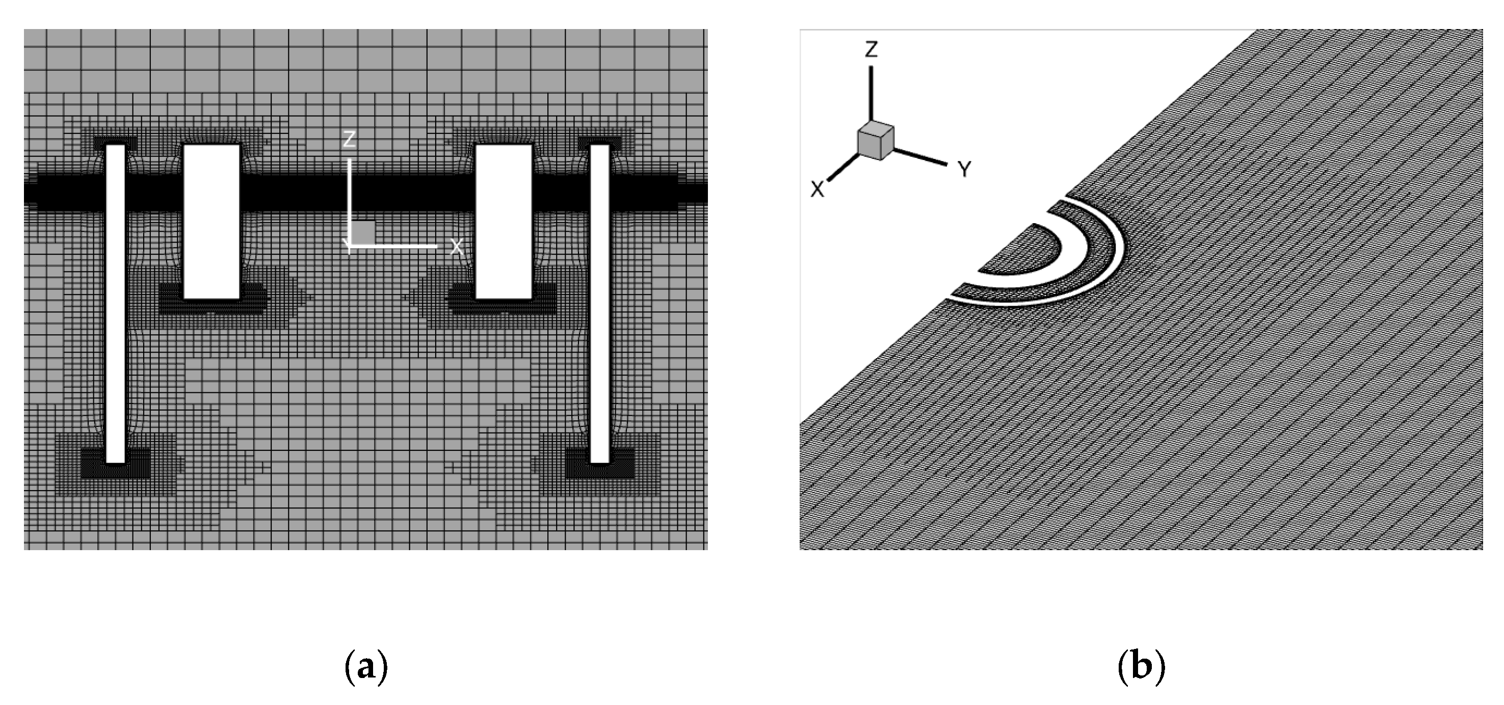
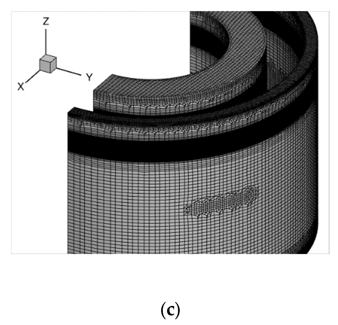
The domain discretization is depicted in Figure 3. The discretization of the domain upwind of the configuration was based on the wave characteristics. Near the free surface, the domain was uniform along the z-axis, with a length that corresponded to 18 cells per wave height. The mesh along the wave propagation was also uniform, with a discretization that corresponded to at least 100 cells per wavelength in each domain for the studied wave frequencies. Furthermore, special care was taken near the sharp edges of the structure, as illustrated in Figure 3a, to account for the flow separation that was expected in these regions. Finally, the mesh coarsened as it reached the lateral and the outflow boundary, to make sure that no wave reflections occurred. In order to capture the viscous effects close to the wall, the first point was placed at 0.5 mm normal to the wall.

Figure 4 presents the grid independency study. The M2 grid has the aforementioned mesh characteristics and a total size of approximately 5 million cells. Additionally, three more grids were examined. The M1 grid consisted of 1.6 million cells. The main difference compared to the M2 grid is that it had 8 cells along the wave height and 50 cells at the smallest wavelength. Furthermore, the characteristic size of the mesh close to the wall is two times larger, compared to the previous mesh. The M2-w mesh had the same characteristics as the M2 grid; however, the first node from the wall was placed at 1 mm normal to the wall. Finally, the M3 had a total size of 8.5 million cells. The M3 grid differed from M2 in the characteristics of the mesh near the structure, as well as upwind of the structure in the direction of the wave propagation. The cells per wave height were the same as M2; the total cells per smallest wavelength were 200; the mesh near the structure had two times smaller characteristic size. From the independency study, the M2, M2-w and M3 produced similar results. The characteristics of the M2 grid were chosen for all simulations. The time discretization was chosen as 1000 timesteps for the corresponding wave period [33].

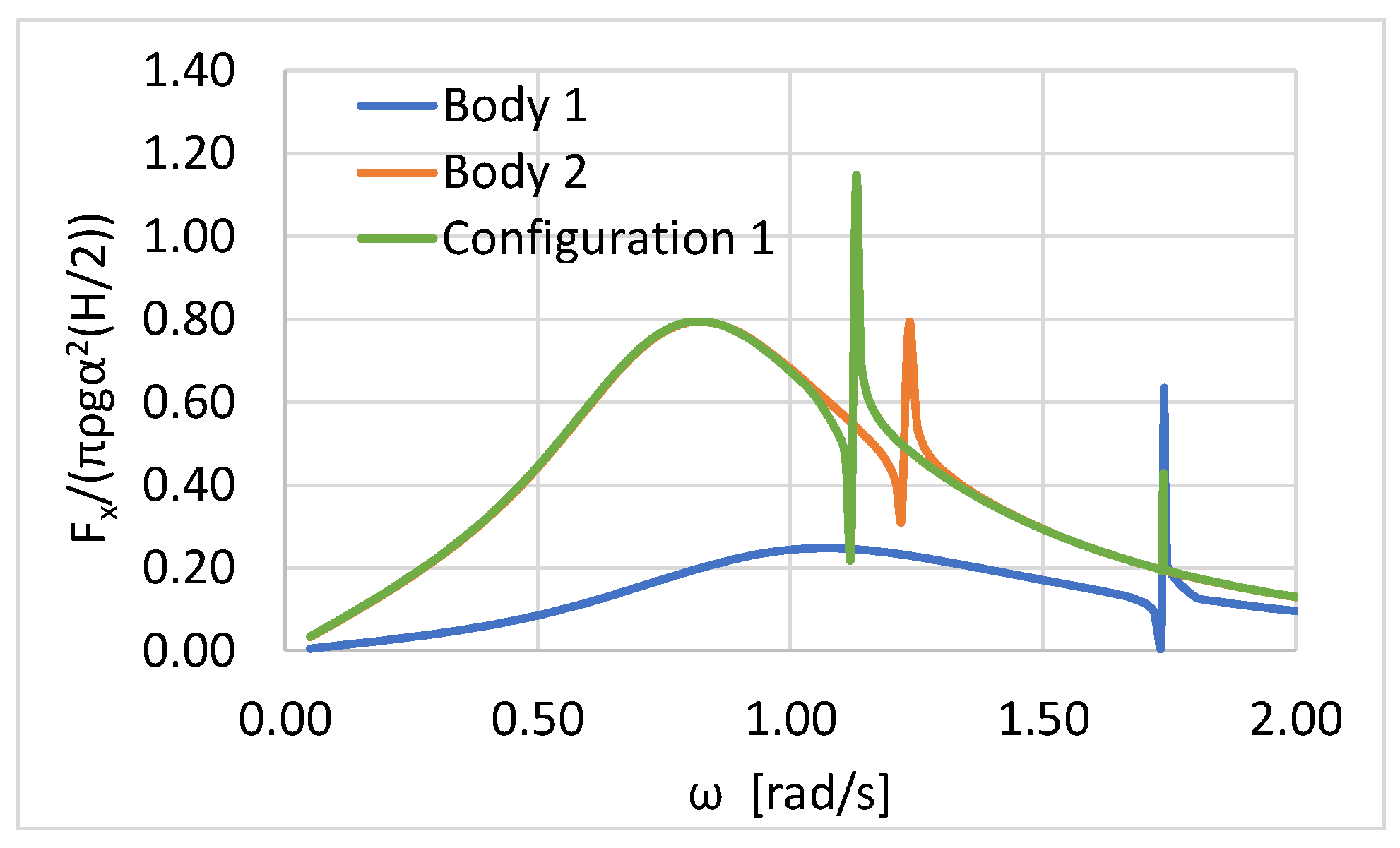
Figure 5 and Figure 6 depict the horizontal and vertical exciting forces on the moonpool floater of the 1st examined Configuration, derived by the presented potential flow formulation. The results are also compared with the corresponding exciting forces on the outer moonpool floater (i.e., Body 2) (see Figure 2a), without the presence of the inner moonpool floater (i.e., Body 1), as well as on Body 1, without the presence of Body 2 (i.e., isolated bodies). The results of the exciting forces are normalized by the term πρgα²(H/2).

The peculiar behavior of the horizontal exciting forces (see Figure 5) on the Body 1 and Body 2, in the neighborhood of ω ~ 1.74 rad/s and ω ~ 1.23 rad/s, respectively, was due to the resonance pitch oscillations of the interior water basin of each Body 1 and 2. The same behavior has been reported in [1] regarding moonpool floaters. It should be further noted that the peculiar behavior of the horizontal exciting force on the total Configuration 1 (i.e., floater of two coaxial, free-surface piercing toroidal cylinders) was moved at a lower wave frequency, i.e., ω ~ 1.13 rad/s. This transpose could be attributed to the annular water area that formed between the two toroidal cylinders, which resonated in a pitch at a lower wave frequency than the corresponding one of the independent moonpool floaters (i.e., Body 1 and Body 2). In addition, a secondary resonance of the horizontal exciting force on the total Configuration 1 was observed in the neighborhood of ω ~ 1.74 rad/s. In the latter wave frequency, the resonance pitch oscillations of the interior water basin inside the Body 1 occurred.

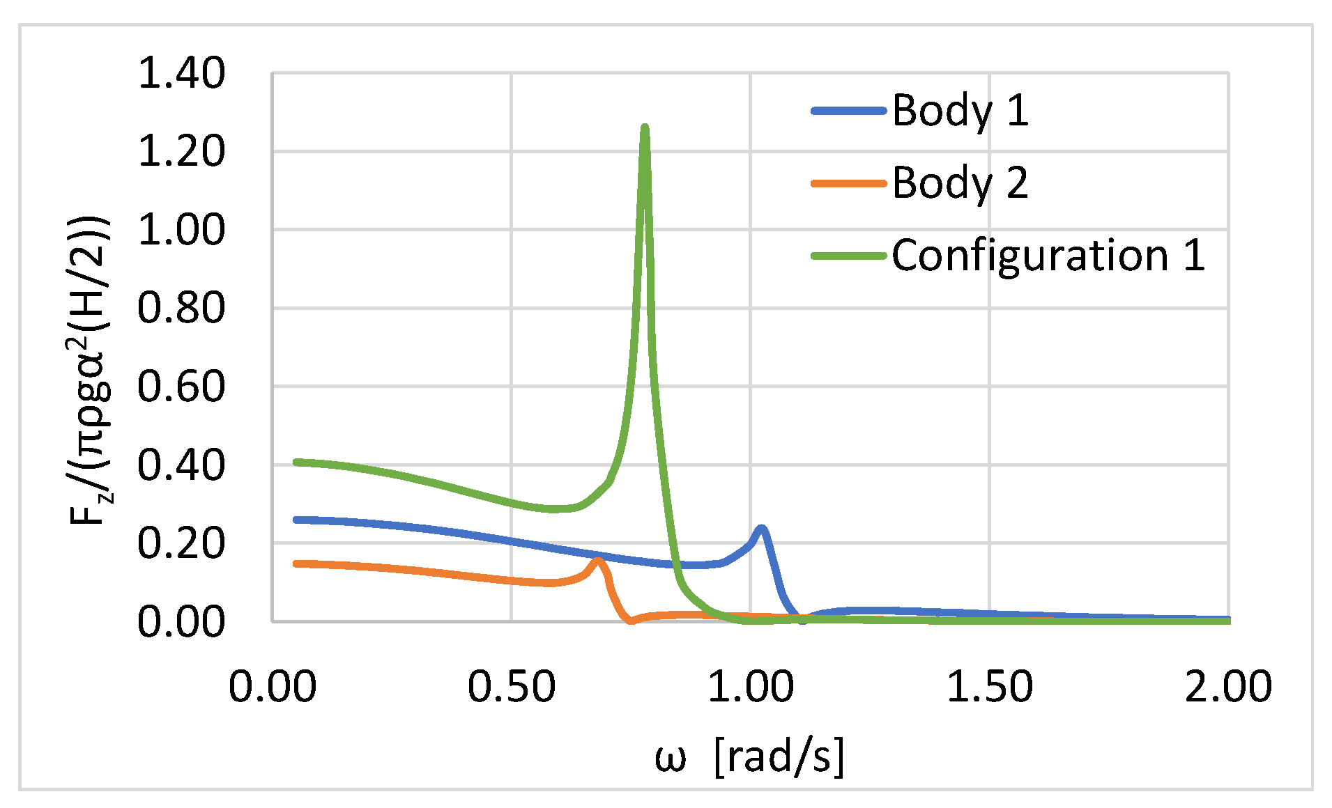
With regard to the vertical forces (see Figure 6) on Body 1 and Body 2, resonances appeared in the vicinity of ω ~ 1.05 rad/s and ω ~ 0.7 rad/s, respectively. These peaks were due to the pumping resonance of the fluid motion in the interior water area of the moonpools Body 1 and Body 2. Concerning the vertical exciting force on the total Configuration 1, it can be seen (Figure 6) that its pumping resonant wave frequency was located in between the corresponding pumping wave frequencies of Body 1 and Body 2 (i.e., ω ~ 0.8 rad/s).

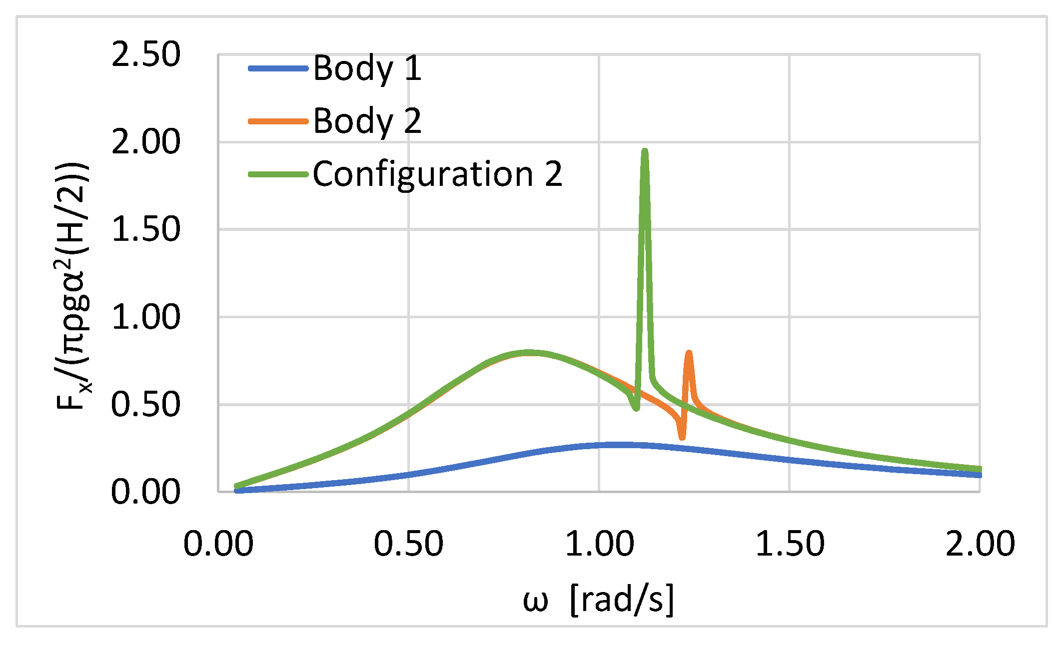
Next, the horizontal and vertical wave exciting forces on the examined Configuration 2 (see Figure 2b), derived from the theoretical formulation, are presented. Specifically, in Figure 7 and Figure 8 the values of F_x/(πρgα²(H/2)) and F_z/(πρgα²(H/2) on the Configuration 2 are depicted, respectively. The results are also compared with the corresponding exciting forces on the isolated Body 1 and Body 2, when the latter were considered alone in the wave field (i.e., Body 1 was assumed alone in the wave field without the presence of Body 2, and vice versa for Body 2).

The resonance of the horizontal exciting force on the Configuration 2 (see Figure 7), which occurred in the neighborhood of ω ~ 1.125 rad/s due to the pitch fluid motion in the annular fluid area between the interior cylinder and the exterior toroidal body, was moved to ω ~ 1.24 rad/s for the Body 2 case, when the latter was assumed isolated in the wave field. As far as the forces on the isolated Body 1 are concerned, it can be seen that they followed a smooth variation pattern at the examined wave frequency range, without any sharp maximizations.

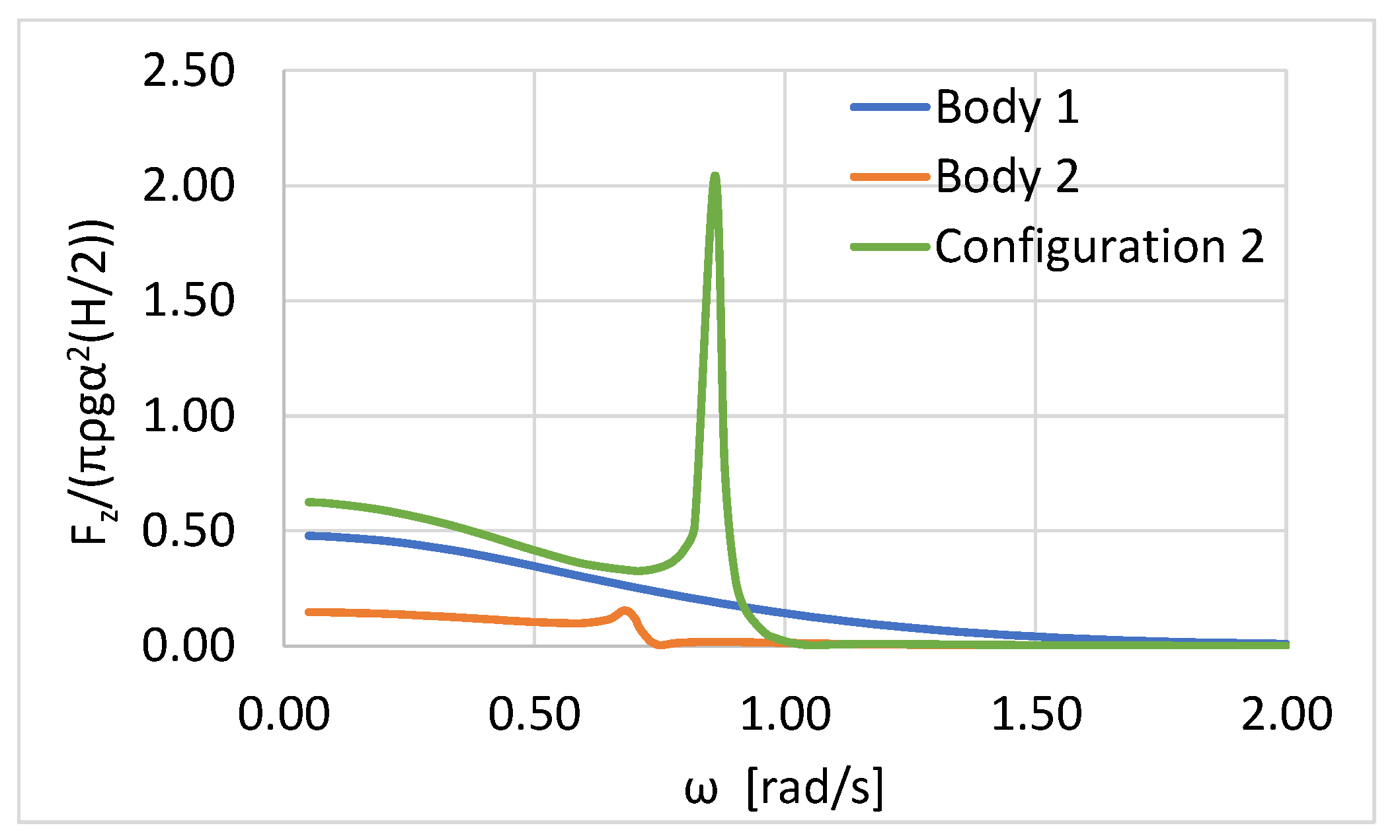
Regarding the vertical exciting forces on the Configuration 2 (see Figure 8), the pumping resonance of the fluid motion in the annular area was depicted at ω ~ 0.85 rad/s [20], whereas, for the isolated Body 2, this pumping resonance lied near ω ~ 0.7 rad/s (see discussion of Figure 5). It should also be noted that the smooth variation pattern of the vertical exciting force on the isolated cylinder follows (i.e., Body 1).

Comparing Figure 5 and Figure 7, it can be concluded that both configurations 1 and 2 attained, in the non-resonance regime, comparable results concerning the horizontal exciting wave forces. Furthermore, their resonance pitch oscillations occurred at the vicinity of ω ~ 1.13 rad/s. Hence, it could be derived that the wave motion inside the pond of Body 1 in the first configuration did not seem to affect the floater’s horizontal forces. On the other hand, the secondary resonance of the horizontal exciting wave force on the Configuration 1 (i.e., ω~1.74 rad/s) was not observed in the case of Configuration 2. Regarding the vertical exciting forces F_z/(πρgα²(H/2)), see Figure 6 and Figure 8; in the case of Configuration 2, due to the truncated inner cylindrical body, they attained higher values compared to the vertical loads on Configuration 1. Hence, assuming both Configurations as heaving point absorbers for wave energy exploitation, Configuration 2 seems to be more efficient compared to Configuration 1.

In the sequel, the results from the theoretical formulation were supplemented by numerical ones, which took into consideration the viscous effects near the sharp edges of the examined moonpool-type floaters. The numerical results presented follow the configuration terminology described in the previous section. A grid consisting of 5 million cells was employed with symmetry conditions (half of the moonpool is modelled). Since the moonpool was considered fixed and the waves were essentially in the linear region, the flow is assumed laminar [29,44].

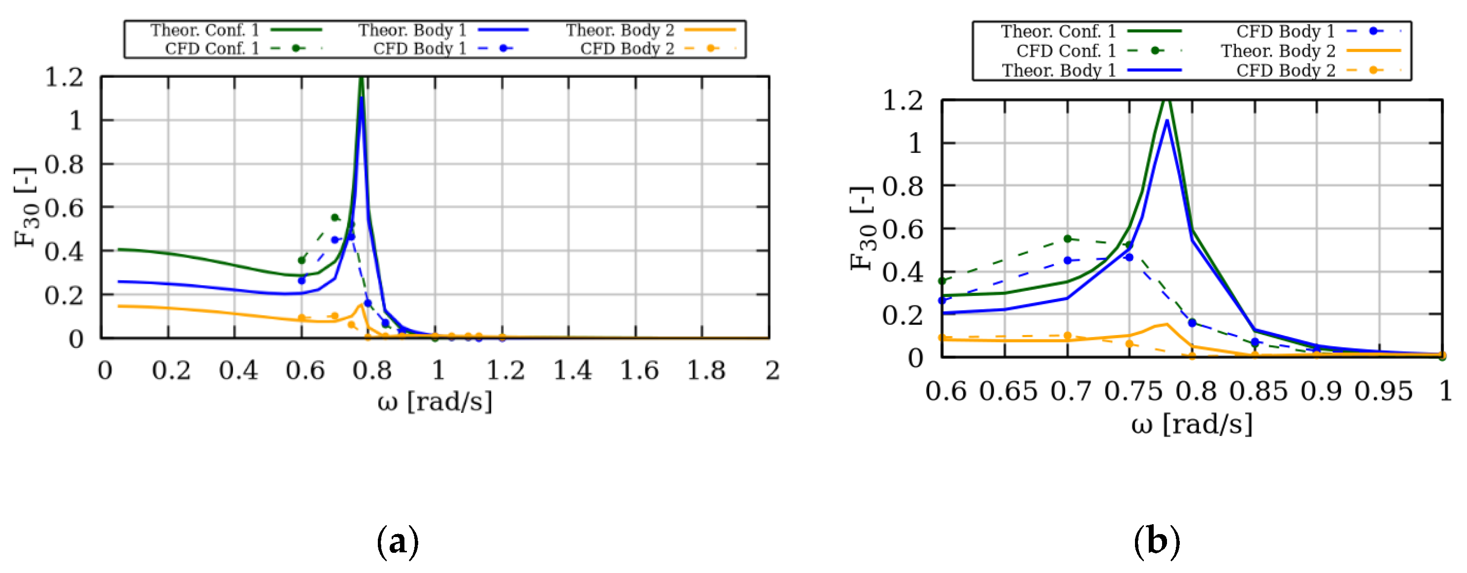
Regarding Configuration 1 the comparison of the non-dimensional horizontal and vertical exciting forces could be seen in Figure 9 and Figure 10. The illustration of the horizontal forces (Figure 9) suggested that the comparison was relatively good for both methods. CFD predictions follow the analytical method’s trends with minor discrepancies. In the proximity of the peak excitation frequency (between 1.0–1.2 rad/s), the differences between the predictions became larger. More specifically, in the near peak frequency region, CFD results predicted earlier the peak of the Body 1 than the analytical method, leading to a rise in total force. At 1.13 rad/s, both methods predicted the maximum horizontal excitation force. However, it was evident that the amplitude of the CFD predictions was significantly smaller. This could be justified by both the phase difference of the peak excitation loads between the two bodies in the CFD predictions (discussed in the following) induced by the viscous effects that were taken into account in the CFD computations.

Regarding the vertical excitation force in Figure 10, the comparison between the methodologies was fair, with the CFD simulations predicting smaller peak loads and shifted towards the lower frequencies. This has also been noted in [29]. Nevertheless, the qualitative comparison for both the total force and the individual body forces was considered to be in good agreement.

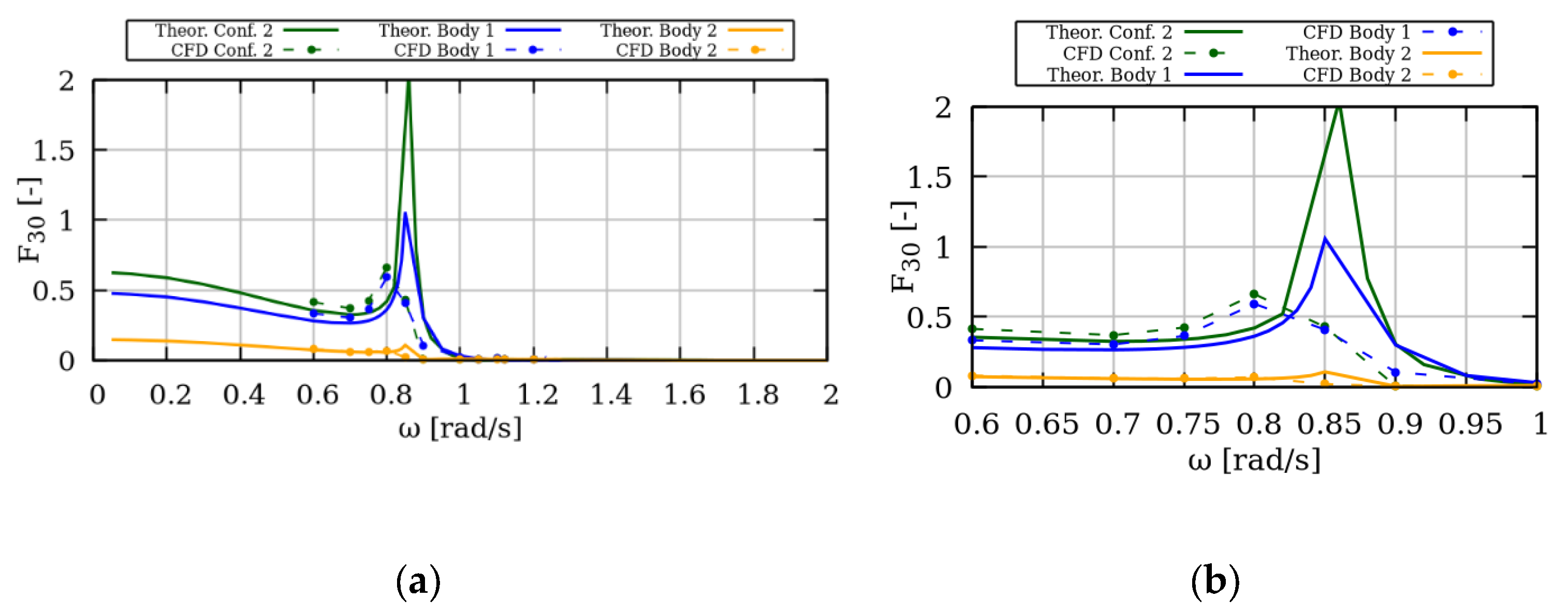
The respective comparison for Configuration 2 (external toroidal cylinder with internal coaxial truncated cylinder) can be found in Figure 11 and Figure 12. The agreement between the numerical results is good in both the horizontal and vertical forces. As Figure 11 suggests, CFD predictions followed the analytical method trends; nevertheless, the peak excitation frequency was predicted earlier. As opposed to Configuration 1, the individual body forces peak excitation frequencies were predicted in the same frequency, suggesting that the forces on the two bodies were in phase. This was also the case for the analytical method’s predictions. Finally, regarding the vertical force in Figure 12, again the CFD predicted the peak excitation frequency earlier; however, as in Configuration 1, the predicted trends were the same.

In order to gain a better insight of this phase difference between each body’s horizontal force in Configuration 1, instantaneous free surface elevation contours at four snapshots of the wave period are presented in Figure 13 at ω = 1.1 rad/s.

As Figure 13 suggests, the sloshing mode was excited between the outer (Body 1) and the inner (Body 2) cylinder, which explains the phase difference between the horizontal force of each individual body.

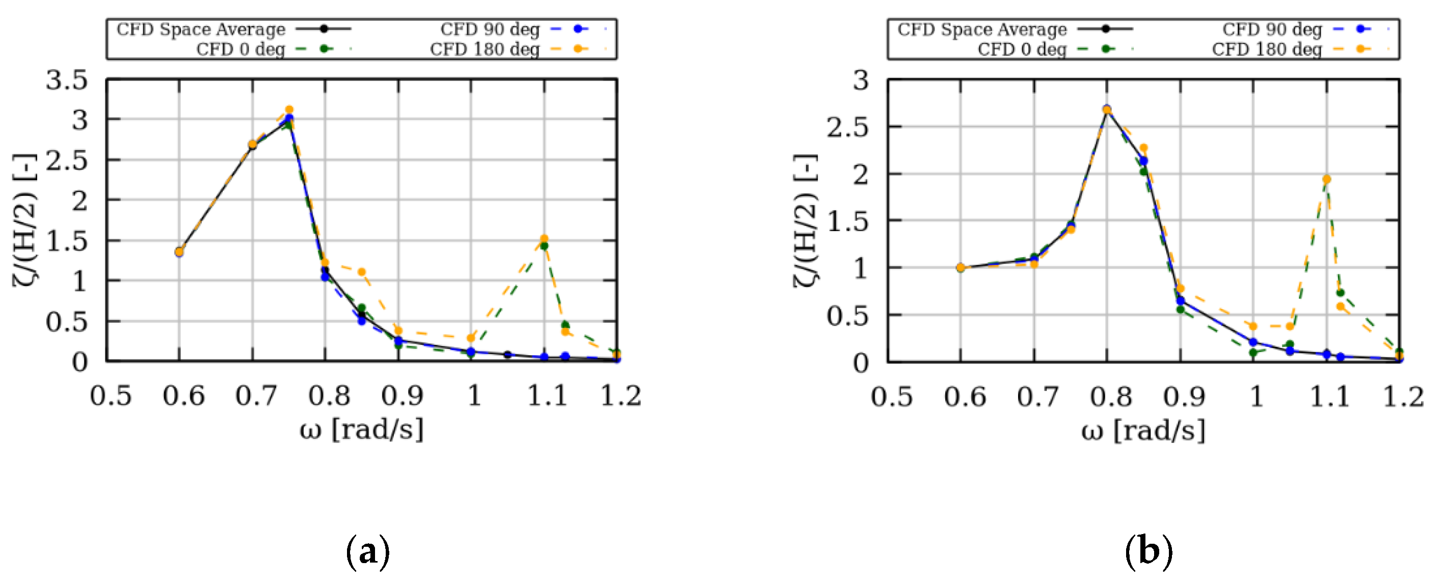
Figure 14 presents the free surface elevations inside the moonpool (between Body 1 and 2) for both configurations with respect to the incident wave frequency. The space averaged free surface elevation inside the moonpool is presented, as well as in three circumferential positions at 0, 90 and 180 degrees (as shown in Figure 13a). In both configurations up to ω = 1 rad/s, it was evident that the free surface elevation did not greatly vary between the various spatial positions, suggesting that the piston mode dominated the free surface elevation inside the moonpool. As the frequency increased beyond 1 rad/s the gauge at 90 degrees followed the spaced averaged elevation; however, the other two locations at 0 and 180 degrees clearly deviated (they increase in amplitude), thus indicating the appearance of a sloshing mode inside the moonpool. As the radial frequency was further increased, this mode dampens out. Furthermore, it is worth noting that peak frequencies of the piston mode resulted in an increase of the vertical forces, while the sloshing mode resulted in the resonance of the horizontal excitation forces.

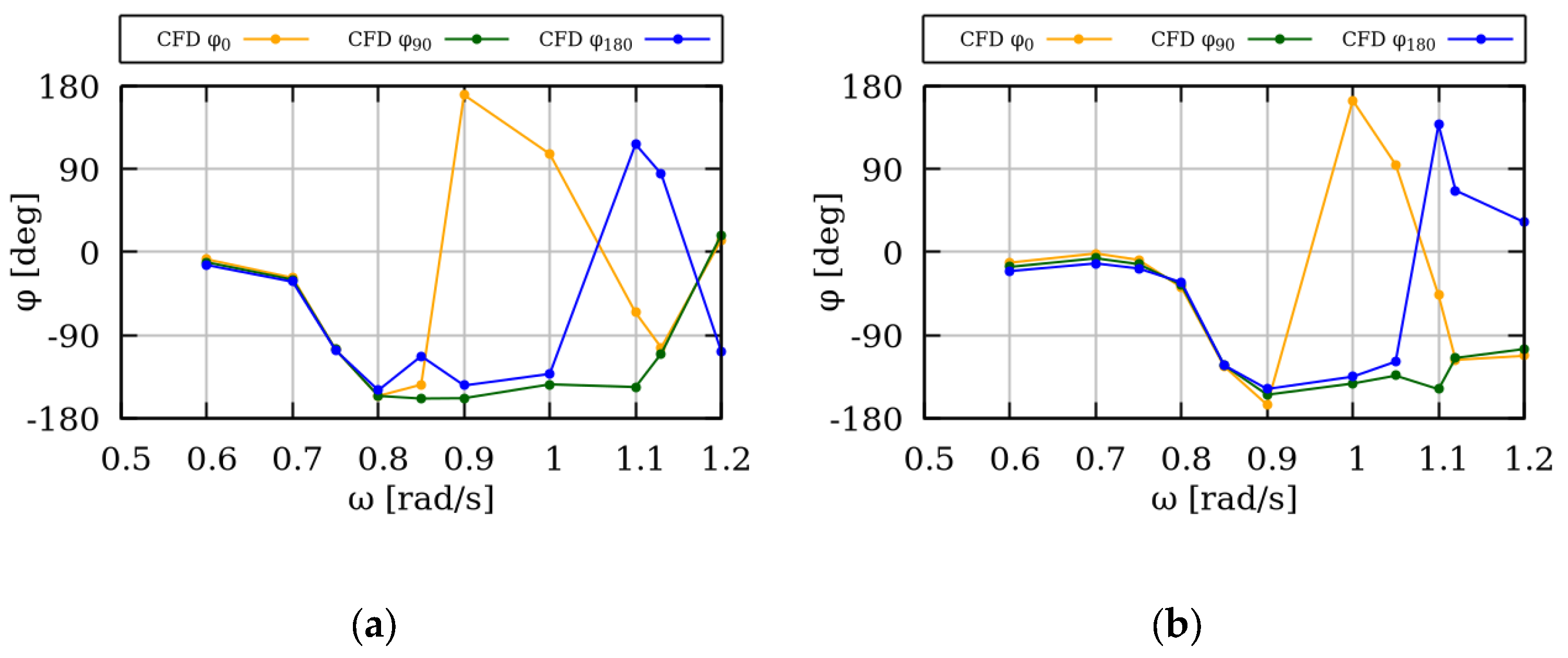
This is further illustrated in Figure 15, where the phase angle of the signal in the three wave gauges is presented. In smaller frequencies, the three signals had no phase difference; however, in larger frequencies, the phases started to deviate. In the case of ω = 1.1 rad/s, the signal in the upwind gauge (0 deg) and in the downwind gauge (180 deg) had a 90 degrees phase difference compared to the middle gauge (90 deg) and 180 degrees between them. In higher frequencies, there were still some phase differences; however, the amplitude of free surface was relatively small (see Figure 13).

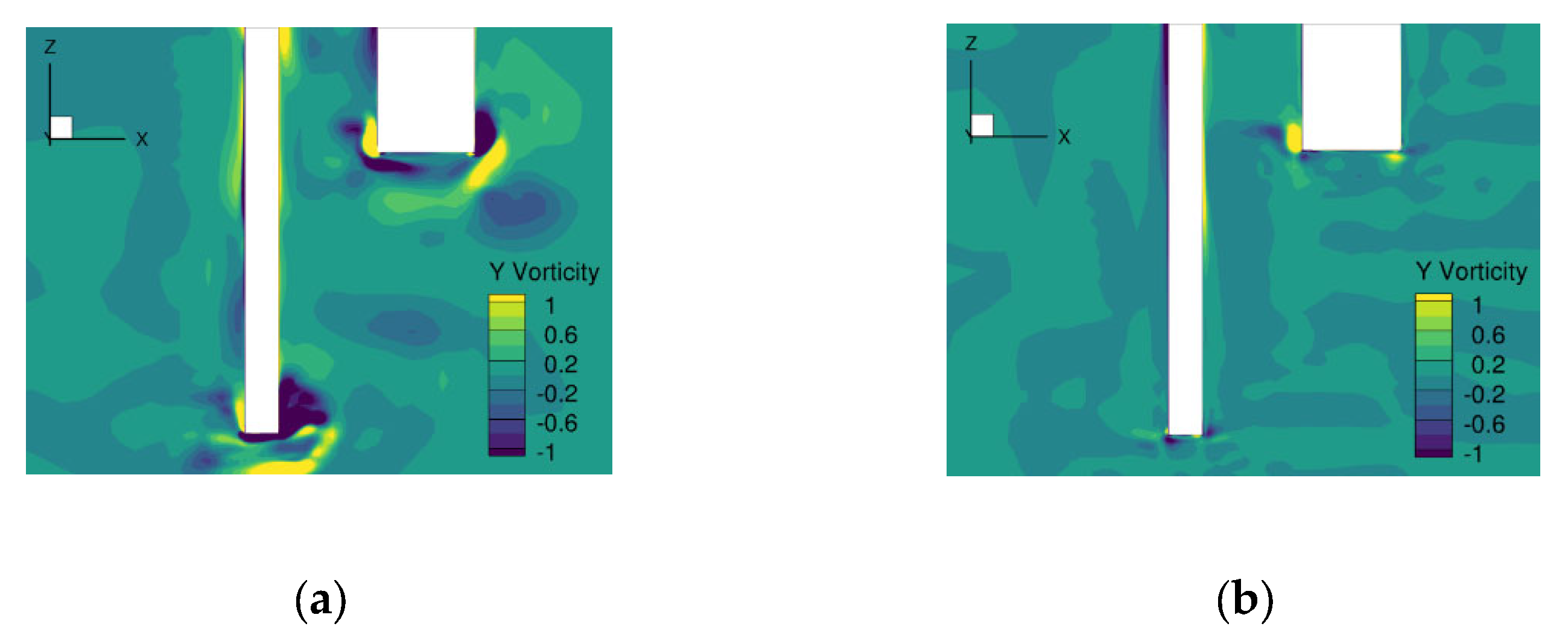
Lastly, Figure 16 presents the y-vorticity field in the symmetry plane in the case of the Configuration 1 for different wave frequencies. Close to the resonance of the piston mode, excessive flow separation was noted near the sharp edges of the structure (Figure 16b). Due to the loss of energy in this region of recirculating flow, the viscous solver predicted smaller amplitude of the piston mode (and thus of the vertical forces) compared to the one of the analytical solution. Contrary to Figure 16b, the vorticity field in larger frequencies (where the amplitude of the piston mode is reduced significantly), the vortex shedding was not significant; thus, minor discrepancies were noted between the two approaches. It was also noted that the performance of inviscid potential models is influenced by the radiation effect of the inner water area, leading to discrepancies between the viscous solver and the analytical solution.

5. Conclusions

A semi-analytical method has been developed to solve the linearized diffraction problem of two types of moonpool floaters, namely: (a) two coaxial toroidal cylinders configuration and (b) a floater encompassed by an external toroidal cylinder and a coaxial internal truncated cylinder. The potential flow theoretical formulation was supplemented by a numerical modelling that considered the viscous effects near the sharp edges of the body as non-negligible.

The accuracy of the two presented methods, the theoretical formulation and the numerical approximation, have been validated in both examined Configurations 1 and 2 and in a wide range of wave frequencies, i.e., 0.6 rad/s to 1.2 rad/s. It can be concluded that, in the non-resonance regime, the comparisons between the two methods were excellent; hence, both models predicted accurate results. However, in the critical wave frequencies near resonance, the CFD modelling predicted the peak excitation frequency earlier, whereas the amplitude of the predictions was significant smaller than the corresponding ones from the theoretical analysis. This can be traced back to the viscous effects that were taken into account in the CFD computations, which altered both the phase difference of the peak excitation loads between the two bodies in the CFD predictions. Specifically, an excessive flow separation was noted in the resonance regime, near the sharp edges of the structure; hence, the viscous solver predicted smaller force amplitudes. On the other hand, in larger frequencies the vortex shedding was negligible; thus, minor discrepancies were noted between the two approaches.

The present research will be continued further by comparing the accuracy of both methodologies to arrays of floating bodies in which the exciting forces on the structures are affected not only by the shape of the floaters but also from their position in the array towards the incoming waves.