Abstract
Hydrogen (H2) can be a promising energy carrier for decarbonizing the economy and especially the transport sector, which is considered as one of the sectors with high carbon emissions due to the extensive use of fossil fuels. H2 is a nontoxic energy carrier that could replace fossil fuels. Fuel Cell Electric Vehicles (FCEVs) can decrease air pollution and reduce greenhouse gases when H2 is produced from Renewable Energy Sources (RES) and at the same time being accessible through a widespread network of Hydrogen Refueling Stations (HRSs). In this study, both the sizing of the equipment and financial analysis were performed for an HRS supplied with H2 from the excess electrical energy of a 10 MW wind park. The aim was to determine the optimum configuration of an HRS under the investigation of six different scenarios with various numbers of FCEVs and monthly demands, as well as ascertaining the economic viability of each examined scenario. The effect of the number of vehicles that the installation can refuel to balance the initial cost of the investment and the fuel cost in remote regions was investigated. The results showed that a wind-powered HRS could be a viable solution when sized appropriately and H2 can be used as a storage mean for the rejected wind energy. It was concluded that scenarios with low FCEVs penetration have low economic performance since the payback period presented significantly high values.
1. Introduction
The ever-increasing needs of modern societies are based on fossil fuels such as oil, coal, and natural gas. Approximately 85% of the worldwide energy used originates from conventional fuels [1]. Thus, the optimal methods to utilize RES are some of the main targets in the energy field (i.e., 2018/2001/EU) to create regions with energy autonomy, sustainability, and a clean environment [2]. Consequently, energy cost is beginning to have a more intensively declining trend. Thus, projects or constructions with a different RES combination are examined to meet energy demand using the most efficient system with less energy deficit and low energy cost.
On the other hand, all countries aim to ensure energy autonomy and sustainability as a tendency to reduce the use of carbon-based fuels and depth in the economy (energy security). In this respect, H2 has been considered one of the best energy carriers as a storage mean for future energy systems. It is clean with high energy content and can be applied in the transportation sector, heating, and electricity generation.
By contrast, H2 does not exist in nature free of bonds. Thus, it is essential to be produced, utilizing existing electrolysis, pyrolysis, and gasification methods. Electrolysis is an electrochemical procedure in which chemical reactions occur with electrical energy as the input energy source [3]. H2 can be produced from low-emission energy sources, mainly by RES, constituting a potential alternative for replacing fossil fuels. On the other hand, HRSs have an important role regarding the distribution infrastructure required for FCEVs. There is to be substantial market penetration of H2-vehicles in transportation while introducing commercial FCEVs, and the corresponding HRSs network must take place simultaneously [4]. In Figure 1, the global electrolysis capacity is depicted, indicating a significant increase from 2018 and onward. In addition, recently announced projects involve utilizing H2 into the gas grid and reducing the emissions in existing installations such as refining and ammonia productions. In addition, it is worth mentioning that some technology developers are pilot-testing electrolysis applications in steel production, leading to a further increase in H2 share in the market. The data for Figure 1 has been derived from the study [5].
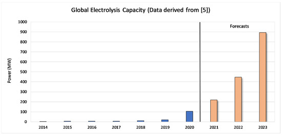
Figure 1.
Constructed HRS and an estimation until 2023 [5].
Worldwide, H2 stations have been built, managed, and designed by universities, research centers, governments, and non-government organizations [6]. Nonetheless, before scaling up the FCEVs market, HRSs should be available in a sufficient capacity supply to fill up the existing vehicles. At this point, a brief description of the HRS is overviewed. The global FCEVs have nearly doubled to 25,210 units at the end of 2019 with 12,350 new vehicles. The United States (US) sales slightly fell in 2019 (reduced to 2100 vehicles in 2019 compared with 2300 vehicles in 2018) (Figure 2). The US remains the world leader in FCEVs, with one in three vehicles being FCEVs, followed by China, Japan, and Korea. Asian countries expanded the number of FCEVs in 2019, reducing the gap with the US. In 2019, the number of new sales reached 700 compared to 600 in 2018. At the same time, the situation in China and Korea is dynamic, rising from a few units in 2017 to almost 5000 in 2019. China has made impressive progress by applying policies that support the adoption of fuel cell buses and light-duty trucks, reaching 4300 and 1800, respectively. Additionally, truck manufacturers are planning to expand these models and start deploying them around Europe and Japan. Figure 2 has been derived considering the data from the study [7].
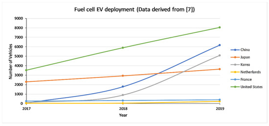
Figure 2.
FCEVs around the world from 2017–2019 [7].
Several studies have been published regarding the HRS and the corresponding H2 specific cost, focusing on these systems to determine the optimum condition for achieving minimum H2 cost. More specifically, Viktorsson et al. [8] proposed a method based on known modelling techniques and evaluated the levelized cost of H2 regarding the decentralization of an HRS located in Belgium. The data provided were attributed to data collection simultaneously with actual cost values. By applying the aforementioned methodology, it was shown that the levelized cost of H2 is 10.3 €/kg considering a lifetime for the HRS around 20 years and an average value of electricity cost of 0.04 €/kWh. Additionally, results regarding the scenario with 80% subsidy showed that the levelized cost of H2 drops to 6.7 €/kg approximately.
Reddi et al. [9] developed a refueling model (based on the Hydrogen Delivery Scenario Analysis Model (HDSAM) tool from the US Department of Energy) to assess the impact of different refueling configurations on the overall cost of HRSs. The study identified that many strategies could be applied to minimize the corresponding fuelling costs. Additionally, it concluded that suitable sizing of high-pressure buffer storage could significantly reduce the compression requirements and the corresponding refueling cost. According to the authors, the solutions that can minimize the refueling cost are: (1) the employment of a tube trailer that fills the vehicle’s tank, (2) the reduction of cut-off pressure of the tube trailer, and (3) the increase of the trailer’s return pressure.
Parks et al. [10] also used the HDSAM combined with the Hydrogen Analysis (H2A) (a model also from the US Department of Energy) to estimate the cost of an HRS consisting of three compressors, five low-pressure cascades (89 kg/unit), three high-pressure cascades (43 kg/unit), and two dispensers (2 hoses/unit). Nevertheless, additional source data were collected via telephone interviews, personal experience, open literature, and manufacturers’ websites. The analysis concluded that the cost of each component was 1.4 M$ for the compressors, 277,000 $ for the low-pressure cascades, 216,000 $ for the high-pressure cascades, and 36,000 $ for the dispensers. The authors compare the pipeline and transportation of cascades tanks by a truck as the main refilling method of HRS. The study concluded that tube trailers have a lower cost, approximately 1.12 $/kg-H2 lower than the pipeline, which costs 2.40 $/kg-H2.
Pratt et al. [11], based on the HRS Analysis Model (HSRAM), investigated different HRS’ scenarios to propose the optimum configuration considering different FCEVs demand profiles or penetration. More precisely, the HRSAM input parameters were overall kept at their default values, while a few parameters were changed for providing a more realistic overview of the problem under examination. From their study, the following conclusions were raised: (a) a significant cost reduction was achieved, when the capacity of HRS increased from 50 to 100 kg/day (estimated cost reduction around 0.93%; (b) for a specific number of hoses and station capacity, gas delivery cascade systems have the lowest cost, followed by liquid delivery cascade systems, while the most expensive equipment is the gas delivery booster systems; (c) the cost of one extra hose (from one to two hoses) is substantially higher for the booster fill systems than for cascade system (liquid or gas); and (d) HRS with a capacity of 300 kg/day and a system with liquid refilling has the lowest initial cost. More specifically, systems with a 200 kg/day capacity have a more increased initial cost than a system consisting of a single-hose dispenser. Furthermore, a configuration with two hoses has a high initial cost, while the gas H2 system is recommended compared to the liquid H2 system.
Rezaei et al. [12] investigated the economic potentials of producing electricity and hydrogen using different wind energy patterns. In their study, the most crucial economic parameters taken into consideration were the levelized cost of wind generated electricity (LCOWE) and levelized cost of wind-based hydrogen (LCOWH), payback period, and the rate of return. Considering the unknown nature of five degradation rates for the wind turbine as well as the five likely rates of future money values the following scenarios were studied: (1) utilization of wind electricity to replace fuel oil electricity, (2) replacement of natural gas electricity, and (3) without taking into account environmental penalties. The results indicated that the LCOWE ranges within 0.0325–0.0755 $/kWh, and the LCOWH ranges between 1.375–1.59 $/kg. Furthermore, the payback period ranges within 2.55–9.48 years throughout the lifetime of the wind power plant and 3.91–8.41 years in the course of the lifetime of a hydrogen production system. In addition, the rate of return for the already mentioned cases will range between 14.15–23.54% and 9.87–21.55$, respectively. The study revealed that electricity generation using wind energy could be a profitable solution, while renewable hydrogen production can offer even better results.
Carr et al. [13] developed an optimization routine to analyze the performance of HRS combined with wind power of total capacity at 225 kW. The system consisted of an electrolyzer with a power output of 270 kW. The refueling station model had been developed using MATLAB, while the time series for the wind power output has been assessed from the UK generic distribution system network. In addition, the time series for the H2 demand is derived from the modified Chevron profile in the H2A analysis. The performance of the optimization routine applied for different examined cases of H2 demand, and wind power has been assessed. Nonetheless, the effect of operating the electrolyzer to minimize wind curtailment in a grid constrained scenario was included. The study found that the optimization routine can increase profits when operating in the market. Still, it depends on various factors, such as the level of H2 demand and wind power.
Qadrdan and Shayegan [14] investigated the cost of building stations simultaneously with the levelized cost of H2 for two types of stations, Steam Methane Reforming (SMR) and electrolysis, with various sizes and capacity factors. In electrolysis, the H2 cost sensitivity to the price of electricity was examined. The analysis concluded that the H2 costs ($/kg) could differ based on station type, size, and capacity factor. H2 production from natural gas presents lower costs ($3–7/kg-H2) compared to electrolysis ($6–10/kg-H2). H2 cost would drop by increasing the capacity factor, but in the case of electrolysis, from a specific capacity factor, H2 cost begins to increase due to the trade-off between the capacity factor and the price of electricity in various load zones.
Considering the already existing work conducted in the specific scientific field, it is concluded that the vast variety of the studies focuses on examining HRS from medium-to-large scale installations. However, a gap in knowledge is identified regarding the HRS in remote regions, a case that will extensively be examined in the current work in terms of refueling capabilities and the corresponding economic viability of each scenario. Moreover, the developed model is separated into two submodels. The first concerns the calculations that should be considered for sizing each component of the system, providing the corresponding mathematical equations and assumptions. The second concerns the economic calculations for evaluating the financial performance for each examined scenario.
2. Research Methodology
The scope of the current work is to evaluate the penetration of FCEVs in remote regions. Prior to this, it is essential to carefully size the HRS to achieve optimal performance in terms of refueling capabilities. The project’s rationale is to utilize the energy surplus from RES (Figure 3) to produce H2 for achieving maximum autonomy in the region (e.g., green island). The stored H2 is used for refueling FCEVs. More specifically, the energy surplus of a 10 MW wind farm, estimated at 81,500 kWh/year, feeds an electrolyzer with a nominal power of 8 MW, producing 47,810 kg-H2 per year [15]. In the problem encountered, it was assumed that the HRS would be refilled once per month. Thus, the storage tank size and the refilling method were determined, assuming a truck transporting liquid H2 to the HRS. The main reason for choosing the specific transportation method relies on the fact that larger amounts of hydrogen can be transported in this form, which is more valid considering the restricted accessibility of a remote region where the construction of pipelines is economically intensive. The methodology developed is separated into two parts. The first one corresponds to the sizing procedure for the various components of HRS. The second part concerns the economic model applied to investigate the economic viability of the installation under different scenarios.
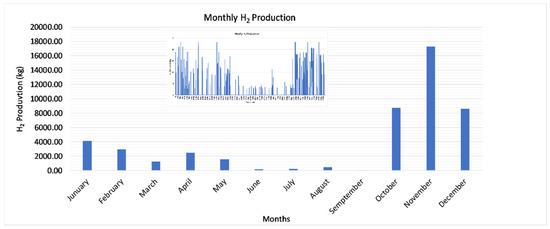
Figure 3.
H2 production from the energy surplus of the wind park on an hourly basis (upper right) and monthly production.
In Figure 3, the monthly H2 production from the wind park’s energy surplus is depicted along with the hourly production pattern derived from the monthly data. The monthly production is used in the sizing procedure since the periods of high demand can be determined for adapting the capabilities of HRS providing a clear view regarding the supply capabilities of the station considering the FCEVs penetration scenarios. The operation of this type of system relies on the utilization of surplus electrical energy rejected by RES in an electrolysis system for the generation of H2 which can be stored in high-pressure tanks or metal hydride canisters for future use. Thus, seasonal demands on H2 could be covered when the overall H2 is insufficient (i.e., the period within June–September).
2.1. Sizing Model
The sizing procedure followed was mainly based on the study of Dikeos et al. [16] and Elgowainy et al. [17] concerning the actual operation of HRS, the various components of the installation, and the model development. Considering the available H2 produced from the excess electricity of the 10 MW wind park, the optimum storage and buffer tank size should be determined to estimate the maximum number of FCEVs that could be refueled. For this purpose, the sizing model of the HRS was based on the tank capacity, the number of dispensers, the buffer capacity, the evaporator capacity, and the pump’s power (see Figure 4). More specifically, the tank capacity depends on the fuel demand; the mass flow rate of the evaporator depends on the demand and the operation hours of the HRS; the pump size is based on the same parameters with the evaporator but also on the size of the evaporator; and the buffer tanks and the dispensers depend on the HOFs number or similarly the number of the FCEVs during the peak hour.
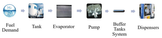
Figure 4.
Main parts of HRS system.
The storage tank capacity (kg) for the HRS to compensate with the demand profile is calculated as:
where is the FCEV’s monthly demand (kg/mo), is the number of FCEVs, and is the scaling factor of tank capacity equal to 1.5. The last parameter is important for avoiding deficits due to an unexpected demand increase since the HRS is supplied once per month. Additionally, tanks are traded with specific capacities (sizes) in the market. Thus, the calculated tank capacity should be close to the available market tank capacity.
The number of buffer tanks (cascades) considers the number of FCEV served under normal time (operation efficiency). Additionally, tanks must be refilled under 700 bar before a FCEV visits the HRS. Cases of refueling simultaneously more than one vehicle should also be considered. Consequently, the Hose Occupied Factor (HOF) is a crucial parameter for the calculation of cascades capacity. The HOF indicates the efficient operation of the HRS, by which the number of dispensers can be estimated. The proper values for HOF are equal to or below 50% (~30 min/h). For this purpose, HOF for each scenario is calculated for determining the optimum number of dispensers by using the equation:
where are the maximum refueled vehicles per hour, is the total occupied hose time (min), and is the number of available hoses at HRS. Considering that dispensers with two hoses were investigated in the six scenarios, half the number of hoses’ dispensers are needed, setting HOF lower than 50% for each scenario (examining ad hoc each case).
The buffer tanks’ capacity is calculated as:
where is the total capacity of all cascades (kg), is the number of available hoses at HRS, and is the capacity of each cascade (buffer tank, kg). The selected capacity of tanks equals 9.4 kg, which is the smallest in the market. However, if we consider that the average FCEV tank capacity is 5 kg, the buffer is able to refuel approximately 2 FCEV. As a result, HRS can deal with even a difficult situation (e.g., islands with high tourism interest).
The evaporator transforms the liquid H2 to gas, while at the same time, it should feed the buffer tanks at an optimum rate. The optimum mass flow rate is evaluated through a minimum flow rate to meet the average demand. During peak hours, the maximum fuel quantity is calculated as an average of the optimal choice to avoid oversizing.
Τhe maximum mass flow rate of the evaporator is calculated as:
where is the number of dispensers of the HRS, is the number of hoses (per dispenser), is the maximum storage capacity of a FCEV, and is the peak hour (s), which equals 1 h as a peak hour/worst case scenario in the particular study.
Accordingly, the minimum mass flow rate is considered as:
where is the mean daily dispensing rate calculated on an annual basis (kg/day) and is the operating hours of the refueling station (h/day).
Pumps are also an important component of the system in which H2 is circulated and stored at a specific pressure range into the cascades. The required power depends on the pressure, the mass flow rate, and the density at operational conditions. The capacity of the evaporators defines the exact specifications of the pump (s). Thus, the power of the pump in conjunction with the flow rate is calculated as:
where is the power requirement of the pump (kW), is the total evaporator mass flow rate (kg/h), is the maximum pressure of cascade storage vessel (kPa), is the H2 supply pressure from the storage tank (kPa), is the density of H2 (kg/m3), and is the pump’s total efficiency.
2.2. Economic Model
The HRS’s economic evaluation considers the initial cost of the investment, the fixed maintenance and operation cost, and the expected annual revenues for calculating the payback period, the Net Present Value (NPV), and the Internal Rate of Return (IRR). The economic model was developed by combining the models proposed by Elgowainy et al. [17] and Kaldellis et al. [18]. Table 1 presents the values of the economic parameters taken into consideration for the case study application.

Table 1.
Economic parameters.
As already mentioned, H2 is transported via trucks in liquid form, which is energy intensive due to low-temperature requirements. Thus, the cost of cryogenic storage tanks includes the installation cost, the transportation cost, the verification of standards, and the regular operation. Therefore, the initial cost for each part of the expenses is given as [17]:
where is the initial cost of the storage tank (€), is the specific cost of the storage tank (€/kg), is the available storage tank capacity (kg), and CEPCI refers to the Chemical Engineering Plant Cost Index, which includes the installation cost, planning, and other costs required for each part of the equipment [17].
where is the initial cost of dispensers (€), is the number of dispensers, is the specific cost of the dispenser (€/unit), and is the level of technological improvement of the components with moderate industry experience [17].
where is the initial cost of cascade system (€), is the total required cascade capacity at a refueling station (kg), and is the specific cost of cascade system (€/kg) [17].
where is the initial cost of an evaporator (€), is the number of evaporators, is the specific cost of an evaporator (€/(kg/h)), is the evaporator’s basic parts’ cost (electric systems, valves, cell, etc., in €), is the total mass flow rate of the evaporator (kg/h), and is the level of technological improvement about components with significant industry experience [17].
where is the initial cost of the pump (€), is the number of pumps, is the specific cost of the pump (€/unit), and is the level of technological improvement about components with limited industry experience.
Considering Equations (7)–(11), the initial cost required for the investment is calculated as:
The fixed operation and maintenance (M&O) costs includes the annual expenses required of the operation of the HRS, i.e., labor, energy, maintenance requirements of the components, the hydrogen supply cost, etc. More precisely, the fixed M&O cost is calculated as:
where is the annual fixed cost of the HRS, is the annual labor cost, is the energy consumption cost, is the H2 selling price from the H2 production station owner, is the cost concerning the fuel losses during HRS operation and refilling, is the insurance costs of HRS, is the O&M cost of the pump, is the O&M cost of storage means, is the O&M cost of the electrical equipment, is the fixed cost of dispensers from O&M, and is the fixed cost of the remainder system from O&M.
More precisely, is calculated by taking into consideration the number of employees, the mean hourly labor cost, and the annual man-hours required. As for the calculation of , the energy consumption of the pump as a major consumption is mainly considered and calculated as:
where is the annual H2 dispensed (kg/year) and is the energy cost purchased from the local electricity network (€/kWh).
The depends on the H2 purchased cost from the H2 production station. The cost from fuel losses is calculated as [19].
where is the purchase price of H2 (€/kg), is the annual fuel losses (kg) due to boil-off (taken as 6% for each refilling), and is the annual fuel losses (kg) during pump operation (calculated as 0.25% per day) [17].
The is considered 1.05% of the initial cost and the 4% of the initial cost. The , , , and are taken as equal to 1% of the initial cost [17]. The present value of the operation and maintenance cost () for years of operation is calculated as [18]:
where is the inflation rate of maintenance and operation cost.
The revenues of the HRS consider the quantity of H2 finally refueling cars, excluding fuel losses, the selling price of fuel, the fuel escalation rate, and the discount rate. Thus, the revenues are calculated as:
where is the annual net income in (€/year), is the annual H2 price escalation rate, and is the discount rate. Specifically, the annual revenues are equal to:
where is the annual H2 sales (kg), is the sale price of H2 (€/kg), and is municipality taxes in euros (taken as 3% of revenues).
By considering the above, the Net Present Value of the investment is calculated as [18]:
where is the obtained subsidies and is the residual value of the investment at the end of its life span (n years).
The profit ratio is related to the growth of the invested capital; thus, it is calculated as [18]:
Finally, the Internal Rate of Return (IRR), used in capital budgeting to estimate the profitability of the potential investments [20], is calculated from the NPV equation defined as the ratio for .
3. Results
3.1. Description of Scenarios
Six scenarios were considered for sizing and evaluating the cost–benefit of an HRS in a remote region. On each occasion, different penetrations of FCEVs and monthly demands were taken into consideration. The values of the parameters presented in Table 2 are what resulted, assuming a fuel consumption of 1.2 kg/100 km [21] with an estimated average covering a distance of ~5000 km/year in remote regions of Greece [22].
Table 2.
Scenarios of demand based on FCEVS penetration.
3.2. Brief Summary of the Main Results
By applying the sizing model for the six different scenarios, the results regarding the tank capacity, the number of dispensers, buffers and evaporators’ capacity, and the required pump’s power are presented in Table 3. Obviously, as the number of FCEVs increases, the corresponding tank capacity should also increase. More specifically, within scenarios 1–3, the tank’s capacity is doubled. Furthermore, between 200 and 250 vehicles, the tank capacity remains the same, as it is able to serve the same number of vehicles. Considering the number of dispensers, there is not any increase in scenarios 1–3, while in scenario 4, two dispensers are required, three dispensers for scenario 5, but four for scenario 6. The buffer’s capacity for scenarios 1–3 is calculated at 18.8 kg, while for scenario 4, it is at 37.6 kg. Additionally, scenarios 5 (Mc = 56.3 kg) and 6 (Mc = 75.1 kg) require essentially higher capacity, as they refer to bigger communities (regions). In the case of evaporators’ capacity, the values range from 42 to 45 kg/h, with scenarios 5 and 6 presenting the same capacity. Concerning the required pump, the power ranges within 69–73 kW. In more detail, scenarios 1 and 2 require pumps of 69 kW power, and scenarios 3 and 4 need pumps of 70 and 71 kW, respectively, while scenarios 5 and 6 require pumps of 73 kW.
Table 3.
Equipment sizing for each scenario.
In this respect, and by considering both the sizing and economic results in Table 3 and Table 4, it is concluded that scenarios 1 and 2 are not economically viable even with 50% subsidy. Nevertheless, the subsidy is a vital prerequisite for constructing an HRS for the rest of the scenarios. One of the parameters that should be considered is the estimated FCEV number (or monthly demand), which is in function with HR’s size, cost, and income. More specifically, when the number of FCEVs increases, so does the specific cost. Thus, it is concluded that HRS should supply a higher number of FCEVs to reduce overall costs. In this sense, the same results are ascertained regarding the rest parameters of the economic model. For example, in scenario 6, in all four subsidy cases, the payback period presents better values than the rest scenarios. In addition, the profit ratio has higher values (equal or above 1) in the cases presenting increased FCEVs penetration. Thus, the economic parameters indicate that high FCEV penetration is necessary to achieve an efficient and economically viable HRS.
Table 4.
Economic results for the six scenarios.
3.3. Discussion
The economic criteria of an investment are the most significant for the discussion and the final decision. Additionally, the minimum size of the equipment required to efficiently service FCEV is another parameter discussed in this section. Isenstadt and Lutsey [23] state that most of the governments invest 2–3 Μ$; however, in their study, they concluded that the overall cost of HRS will drop to 1 M$ approximately. They estimate that the specific cost of H2 production fluctuates from 4 to 10 $/kg. Obviously, an increase in fuel demand affects the initial cost (see Figure 5), but it has the opposite result to specific costs. Additionally, some basic parameters that can cause cost reduction are the H2 market spread and technology evolution. Comparing this range of costs with the results of the current study, it can be concluded that the results are in good agreement with the results obtained by other researchers for most of the examined scenarios. The values of Figure 5 has been derived from the study [23].
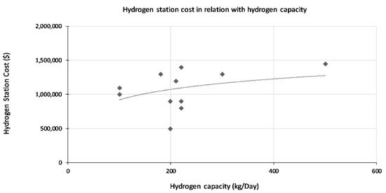
Figure 5.
Effect of H2 demand on initial investment cost [23].
There are three HRS types: Gas-H2 refills, the first HRS type, dispense (or store) 180 kg/day (average price), and the total cost of HRS construction is 2 M$ (1.7 M€). The second type is the Liquid-H2 (LH2) delivery, and the differences in the equipment of HRS reduce the cost of the station. This kind of station can dispense 350 kg/day, but ICo is higher than the first one (2.8 M$). Nevertheless, the high capacity of HRS, with liquid-H2, causes a significantly lower ratio of cost per kg of H2. The most cost intensive kind of station is the HRS with onsite production of H2. Capacity is limited, but the equipment is also more complicated and extraordinary (cost intensive). The capacity is only 120 kg/day, and the total cost equals 3.2 Μ$ [24].
Taking into consideration the above average values, a ratio of cost per kg can be calculated to compare with the results of this research. Especially, HRS with gas-H2 has a capacity equal to 65,700 kg annually (maximum). Based on cost and capacity, the specific cost is estimated at 14.42 €/kg. As for HRS, which stores LH2 in its tank, IC equals 2.38 M€ (2.8 M$), but its capacity is 350 kg/day or 127,750 kg/year. Consequently, the specific cost is significantly lower than gas-H2 (10.63 €/kg). The most cost intensive project is HRS with onsite production, as it is already mentioned. The tank of this station can refuel FCEV with 120 kg/day or 43,200 kg/year due to the production part, which restrains the required space. As a result, the specific cost equals 30.51 €/kg, which is considered very high. Nevertheless, it is an objective discussion to consider which type of HRS is optimal since many factors and indicators should be estimated and evaluated.
Comparing the above values with the last scenario (indicatively) of this research is compelling for determining the meaning of results and ensuring credibility, as it has the highest capacity (or demand). Based on the results of the sixth scenario, the annual fuel demand equals 16,900 kg/year (or annual H2 stored 26,600 kg/year), and the capital cost is ~€694,000 (no subsidy). Consequently, the specific cost of HRS is 12.8 €/kg for this occasion. In case there is a subsidy, the specific cost can be essentially reduced, and it would be equal to 11.5 €/kg with 50% subsidy. Compared with 10.6 €/kg of relative example with LH2 (above), there is an essential declination between the two values (without subsidy). However, it should be considered that this HRS was considered to be constructed in a remote region of Greece, which means that transfer of equipment would be cost intensive. In addition, low fuel demand is the main cause of this project’s low income, and the H2 production station was considered to be far from HRS, close to the wind park. Consequently, these factors affect the cost degree of HRS during its construction (and operation); therefore, there is a +14% burden. On the other hand, it is still an alluring investment compared to the average price of the three examples (above), which is 18.3 €/kg. Last but not least, the first project in an upcoming field is usually subsidized by a government and as a result possibility for profitability (viable investment) and motivation of an investor are considerable in a Greek remote region.
On the other hand, the cost for the vehicle owners is crucial for the spread of “green vehicles” in the market, as it indicates the ability of H2 to compete with fossil fuels and motivates the market to purchase FCEV. Additionally, it is essential for the investment risk, which is high for investments in remote regions (in general). Based on the Shell H2 study [25], petrol vehicles seem to be the most cost intensive due to fuel efficiency. Especially, Battery Electrical Vehicles (BEV) cost the owner about ~6 € per 100 km in contrast with a conventional car, which demands approximately 9 € per 100 km. As for FCEV, they cost 6.1 € per 100 km (forecasting for 4.5 €/100 km). According to Kolb et al. [26], diesel is the only fuel that approaches the cost of FCEV and BEV. Specifically, 6.3 € per 100 km are required for a diesel vehicle. Nevertheless, emissions indicate a decreasing usage of fossil fuels (mainly diesel). Additionally, their price is vulnerable to unexpectancies, i.e., wars, accidents, COVID-19, etc. Additionally, Shell hydrogen study [25] states a future projection (2030) of fuel cost for vehicles, which indicates that declination between petrol vehicles and FCEV-EV will be increased by a factor of 2.5 times. That said, the cost for FCEV and EV owners will be equal (approximately), as FCEVs have a greater fuel range (see Figure 6). Figure 6 has been derived considering the data from the study [25].
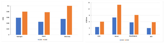
Figure 6.
Fuel cost per 100 km for petrol vehicles, hybrid vehicles, EV, and FCEV in 2020–2030 [26].
Considering the results of this research, Table 4 indicates the fluctuation of cost per 100 km among six scenarios. Focusing on scenarios 3–6, which will have capital growth, fuel costs are ~7 €/100 km (average). There is a considerable decline (~13% burden) when the average value of these scenarios is compared with 6.1 €/100 km [25]. Another parameter, which configures the weight of subsidization in the spread of H2 in Greece, is the cost/100 km which indicates the advantage of H2 compared to other conventional fossil fuels, especially in the remote rural regions. Even if the first discussion for HRS’s construction (LH2) in a remote Greek region seems to be profitable at some point (petrol: 14.8 €/100 km), more aspects should be considered, such as cost for vehicle owners. Thus, the role of the Greek government (consider an economic crisis) is to finance HRS construction and acquisition of FCEV (or reduce cost by another method) to motivate investors and habitants of remote regions.
From an economic perspective, the cost/100 km constitutes a reliable parameter for determining which is the most economically viable solution. More precisely, the average cost for a remote user is 7 €/100 km approximately while the average world values are at 6.1 €/100 km, ensuring that H2 is a competitive fuel even if HRS locates in remote regions. Consequently, it can motivate the replacement of conventional vehicles, considering the cost of the fossil fuels for vehicles owners (9–14.5 €/100 km). Focusing on the investor’s cost, the energy cost of HRS (from a pump) is 0.25 €/kg vs. 0.23 €/kg (world average). Especially, the total cost for the investor (specific cost of HRS) equals 12.9 €/kg in a remote region, which is 19% higher than the world average cost (future projection: 6.2 €/kg). Thus, there is a considerable difference, mainly from the obstacles of a remote location, such as the equipment transportation in a distanced location. Additionally, the number of FCEVs is confined in a remote region compared to a city, which can cause low income for an HRS and a high cost of fuel.
As for the sizing results, monthly demand determines the size of equipment. Consequently, the storage tank is the main component that can vary in each scenario to meet the refueling requirements. As previously mentioned, the storage tank is increased by 50% approximately when the number of FCEVs is doubled. In addition, the buffer tanks capacity between 25 and 100 FCEVs is about 18.8 kg. In the fourth scenario, a buffer tank with a capacity of around 37.6 kg is required, indicating that the size is doubled over 100 vehicles. For scenarios 5 and 6, the capacity is increased by about 25% compared with scenarios 3 and 4. The main tool for HRS sizing and evaluation of its operational efficiency is HOF. More precisely, the first case examined was with one dispenser for scenarios 1, 2, and 3. More specifically, in scenarios 1 and 2, HOF is 16% and 33%, respectively. In the third scenario, HOF equals 65%, indicating that two dispensers would be a proper solution for reducing the HOF index below or equal to 50%. However, economic indicators can significantly affect the final choice regarding the equipment that is applied. Overall, installing one dispenser seems to be the optimum solution for scenarios 1 and 2 (Figure 7).
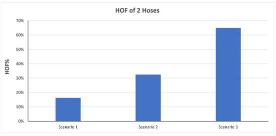
Figure 7.
HOF indicator for 1 dispenser.
In Figure 8, the case with two dispensers for all six scenarios was examined. Nonetheless, the application of two dispensers seems to be an oversized solution for scenarios 1 and 2 since HOF is about 8% and 16%, respectively. In addition, scenario 3 presented an improvement reaching HOF around 30%, while scenario 4 presents HOF at 49%. Moreover, scenarios 5 and 6 present HOF at 65% and 81%, indicating that more dispensers are required.
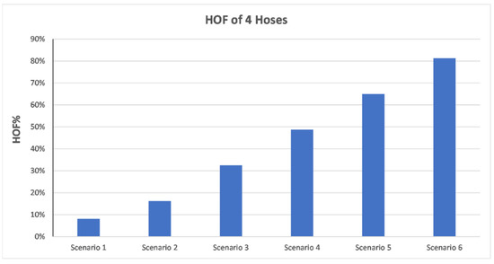
Figure 8.
HOF indicator for 2 dispensers.
In Figure 9, three dispensers for all six scenarios were examined, and it is concluded that the system in scenarios 1, 2, and 3 have been oversized. However, a significant improvement is noted in scenarios 4 and 5, reducing the HOF index from 49% to 33% and from 65% to 43%. However, scenario 6 presents a high HOF index indicating that a solution with four dispensers could be more appropriate.
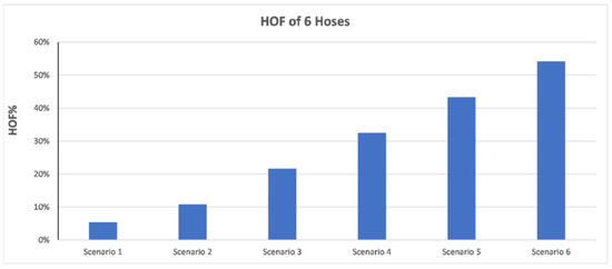
Figure 9.
HOF indicator for 3 dispensers.
Finally, four dispensers for all six scenarios were examined. From Figure 10, it is concluded that the HOF index has been within legitimate limits. Thus, this solution can be characterized as economically viable since the specific cost has not increased significantly. Nevertheless, in scenario 6, the HOF index was reduced to 41%. However, as mentioned previously, this scenario could be economically viable in developing regions with higher FCEV penetration.
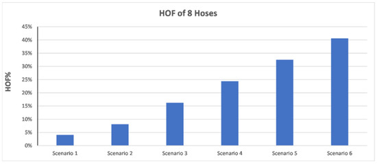
Figure 10.
HOF indicator for 4 dispensers.
The cryopumps are the most cost intensive part of the equipment reaching almost 32% of the total invested capital. Thus, due to the low number of FCEVs in remote regions, one pump is suggested. In this respect, the optimum tank capacity in relation to the number of vehicles that will be refueled can be determined. It should be considered that vessels can be found in the market in standard specific volumes, usually resulting in an oversized tank. Moreover, the number of dispensers is a crucial selection because this component balances the service time of FCEV, the cost of the equipment, and the forecasting for the fuel demand on a life cycle basis. The main criterion for this decision is the HOF, which should remain lower than 50%. However, this study focuses on remote regions where an increase in fuel demand seems to be impossible based on population and market capabilities.
The cost of fuel, the selling price, and the corresponding payback period, IRR, and profit ratio for all six different scenarios considering various subsidy values were also investigated. By taking into consideration Figure 11, it is concluded that increasing the demand reduces the cost of H2. This implies that the size of the equipment applied in the HRS can affect the corresponding revenues. One thing that should also be considered is that, as the subsidy increases, the cost of H2 decreases, highlighting that novel technologies should be supported.
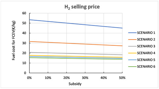
Figure 11.
Effect of subsidy on the final selling price of H2.
The analysis of initial cost, maintenance and operation costs, and the revenues on 20 years base can ensure the possibilities for the profitability of each scenario. However, it should be considered that the long-term evaluation can have significant deviations, which depend on the assumptions, reliability of data, and unexpected changes in the economy (market) and technology. Thus, a comparison between costs and revenues is beneficial (Figure 12) in which the payback period is indicated with bullets.
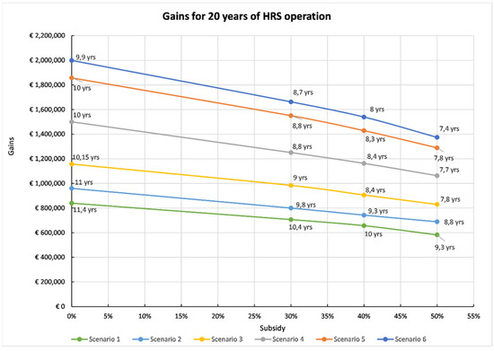
Figure 12.
Effect of subsidy on payback period. Text on the bullets presents the payback period for each scenario and case examined.
In scenario 1, the payback period ranges between 9.3 and 11.4 years (approximately), while the subsidy significantly affects the repayment of invested capital. In scenario 2, higher revenues are presented, and the payback period ranges from 8.8 to 11 years. Additionally, the economic support by the government has a vital role in minimizing the payback period. In scenario 3, the payback period is about 10.2 years without subsidy. Despite that, the payback period can be reduced to 7.8 years, with a subsidy at 50% approximately, motivating the investor for the specific scenario. Similar results are presented in scenario 4, while in scenarios 5 and 6, revenues are significantly increased compared to the third and fourth scenarios. Further evaluation should be conducted considering the values of IRR and PR for providing more accurate results. Scenario 1 presents low IRR and profit ratio values, indicating that the specific solution is not economically viable even if the subsidy reaches 50%, as presented in Figure 13 and Figure 14. Furthermore, similar results are obtained for scenario 2, although it presents slightly improved economic performance.
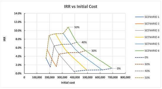
Figure 13.
Effect of subsidy to IRR and the initial cost of the HRS.
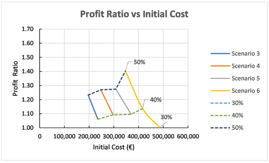
Figure 14.
Effect of subsidy to PR and the initial cost of the HRS.
On the other hand, scenario 3 is the first one to be considered as a profitable one. However, at least a 35–40% subsidy is required to increase the initial value of the investment. In scenario 3, there is 6% capital growth when the subsidy reaches 40% (IRR = 6.4%). On the other hand, with a 50% subsidy, the growth increases by 2%. In addition, the profit ratio takes values above 1, indicating the economic viability of the specific scheme (Figure 13). In the fourth scenario, a growth of the invested capital is presented compared with the third scenario, starting when the subsidy reaches 40%. Specifically, there is a 27% increase in PR value in conjunction with IRR (50% subsidize), which equals 9.3%, while the PR presents higher values than scenario 3. In scenario 5, there are slight differences in comparison with scenarios 3 and 4; thus, it can be considered as equal. Finally, in scenario 6, significant outcomes are presented considering a subsidy of 30% or less, presenting a maximum PR value around 1.40, indicating that the specific solution is the most economically viable.
As for the future of investments in remote regions, estimations could only be made. Because this technology is becoming more efficient (year by year) in all parts of its life cycle, the cost has significant possibilities to be reduced. Additionally, the spread and the evolution of other technologies affect the cost of H2. For example, more and more wind turbines are installed with high efficiency in many remote regions. This study also proves that the burden is the initial cost of the investment and, under appropriate conditions/arrangements, can be affordable (economic efficiency and penetration in the market).
4. Conclusions
The current work focuses on the examination of the performance of an HRS located in a remote region. For this scope, six different scenarios with various FCEVs penetration values and monthly demand were studied to determine the optimum equipment size and economic viability performance. Considering the results regarding the equipment size, demand is a crucial parameter that specifies the size of the equipment. In this respect, tanks capacity is one of the system’s most critical components that should be considered when sizing HRS. The study results showed that the storage tank capacity was increased by 50% when the number of FCEVs doubled. In the case of the buffer storage tank, a demand between 25 and 100 FCEVs (scenarios 1–3), a capacity of 18.8 kg, is appropriate. By contrast, in the case of 150 vehicles (scenario 4), a capacity of 37.6 kg is required. In addition, by comparing the last two scenarios (5 and 6) with a demand of 200 and 250 FCEVs, a 33% higher capacity is required. However, one of the most major parameters used for evaluating the refueling performance of the HRS was the HOF, which should be equal to or below 50%. In this regard, various scenarios were examined considering different dispensers’ quantities.
In this context, an economic analysis was conducted to examine the HRS’s economic viability for the payback period, IRR, and profit ratio. More precisely, the payback period (Figure 12) presented a better performance for scenarios 3–6, amortizing the initial cost of the investment on the (~10 years) with no subsidy. Nevertheless, the percentage of subsidy in which the installation will be financed has a vital role. Thus, installations of this type should be encouraged. Consequently, the results presented regarding the initial cost and IRR (Figure 13) are significant, considering the results provided in the payback period analysis. Nonetheless, better economic performances are introduced at subsidy levels around 30%. Moreover,, the profit ratio has better performance for scenarios 3–6, especially when the subsidy percentage is at 30% approximately. In more detail, scenario 3, in the case of subsidy at 30%, presents a profit ratio around 0.9 which is not into the accepted values. However, scenarios 4–6 present significant good profit ratio values at 30% subsidy. On the other hand, scenarios 1 and 2 have substantially low profit ratio values even when the subsidy reaches 50%, indicating that scenarios 1 and 2 should be rejected. More specifically, the average fixed cost and revenues values for all six scenarios with 0% subsidy were presented. Scenario 1 has an FC of 76.064 € and R around 135.746 €. Scenario 2 has an FC of 94.696 € and R around 160.887 €. Scenario 3 has an FC of 131.761 € and R around 210.055 €. Scenario 4 has an FC of 170.888 € and R around 270.732 €. Scenario 5 has an FC of 213.084 € and R around 335.588 €. Scenario 6 has an FC of 246.336 € and R around 376.423 €. Considering the data derived from the aforementioned analysis, it has been shown that scenario 3 is the most suitable compared to all six scenarios. This statement results from the fact that the number of FCEVs penetration in scenario 3 reflects the conditions occurring in a remote region more realistically. At the same time, economic efficiency considering the parameters of the payback period, profit ratio, and internal rate of return is improved. HRS is a novel technology that can significantly contribute to minimizing conventional vehicles, turning the transportation sector into a green one. For this purpose, HRS should be supported for achieving a higher share in the market. For accomplishing deployment on HRS, some major drawbacks should be resolved. Continuous efforts are made to address these challenges and can be separated into four levels. The first one concerns the HRS equipment technology developments to provide more efficient and cost-effective station operation. The main drawback is the significantly high cost to procure the equipment and the fact that individual HRS are facing issues maintaining high levels of reliability. However, scaling up can improve the economy and reduce cost. Thus, subsidy is a parameter of relatively high importance. The influence of subsidy on IRR and profit ratio can be obtained in Figure 13 and Figure 14. The second level concerns the optimization of supply chain and logistical operation improvements to deliver more cost-effective station capital, operating cost, and lower cost of fuel supply. One popular solution that has been developed relies on high-capacity HRS based on liquid H2 distribution and on-site bulk storage. With this method, a single trailer can carry much more hydrogen than conventional compressed gas transportation. However, the HRS should be carefully balanced to achieve a virtuous equilibrium between demand and supply with liquid H2. The third level issues the policies that should be applied to support HRS and enable demand growth to minimize financial risk. In this respect, programs that support this industry should be prioritized. It is worth mentioning that there is a constantly increased consensus that concerted focus followed with support for H2 infrastructure development at the early steps of the market can lead to a financially self-sustaining industry. The last and fourth level relies on the development of awareness and acceptance with HRS and FCEVs. Furthermore, local permits and governing structures vary from country to country. Thus, the lack of acceptance with hydrogen technologies (i.e., electrolysis and fuel cell systems) due to fear and absence of knowledge can cause delays in the station development. For this purpose, efforts are made to address this gap in knowledge for either electrolysis, fuel cell systems, or FCEVs.
Author Contributions
Conceptualization, K.A.K.; methodology, K.A.K. and V.K.; software, K.A.K. and V.K.; validation; K.A.K. and V.K.; formal analysis, K.A.K. and V.K.; investigation, K.A.K. and V.K.; resources, K.A.K. and V.K.; data curation, K.A.K. and V.K.; writing—original draft preparation, K.A.K., V.K. and S.T.; writing—review and editing, K.A.K., V.K. and S.T.; visualization, K.A.K., V.K. and S.T.; supervision, K.A.K.; project administration K.A.K.; funding acquisition, K.A.K. All authors have read and agreed to the published version of the manuscript.
Funding
This research received no external funding.
Institutional Review Board Statement
Not applicable.
Informed Consent Statement
Not applicable.
Data Availability Statement
The study did not report any data.
Conflicts of Interest
The authors declare no conflict of interest.
Abbreviations
| CEPCI | Chemical Engineering Plant Cost Index |
| EV | Electric Vehicle |
| FCEV | Fuel Cell Electric Vehicles |
| H2A | Hydrogen Analysis |
| HDSAM | Hydrogen Delivery Scenario Analysis Model |
| HOF | Hose Occupied Fraction |
| HRS | Hydrogen Refueling Station |
| HSRAM | Hydrogen Refueling Station Analysis Model |
| IRR | Internal Rate of Return |
| LCOWE | Levelized Cost of Wind Generated Electricity |
| LCOWH | Levelized Cost of Wind Based Hydrogen |
| NPV | Net Present Value |
| PR | Profit Ratio |
| RES | Renewable Energy Sources |
| SMR | Steam Methane Reforming |
Nomenclature
| cb,e | evaporator’s basic parts’ cost | € |
| ce | energy cost | €/kWh |
| purchase price of H2 | €/kg | |
| cs | selling price or specific cost | €/kWh |
| cmunic. | municipal taxes | € |
| co | specific cost of H2 | €/kg |
| e | annual H2 price escalation rate | |
| FC | present value of the operation and maintenance cost | € |
| FC0 | annual fixed cost of the HRS | €/year |
| FCDIS | fixed cost of dispensers from O&M | €/year |
| FCE | energy cost | €/year |
| FCEM | O&M cost of the electrical equipment | €/year |
| FCFC | H2 selling price from the H2 production station owner | €/year |
| FCFCL | cost concerning the fuel losses during HRS operation and refilling | €/year |
| FCIN | insurance of HRS | €/year |
| FCL | annual labor cost | €/year |
| FCPUMP | O&M cost of pumps | €/year |
| FCR | fixed cost of the remainder system from O&M | €/year |
| FCST | O&M cost of storage means | €/year |
| ft | scaling factor of tank capacity | |
| g | inflation rate of maintenance and operation cost | |
| i | discount rate | |
| ic,c | specific cost of cascade system | €/kg |
| ic,d | specific cost of the dispenser | €/unit |
| ic,e | specific cost of an evaporator | €/(kg/h) |
| ic,p | specific cost of pump | €/unit |
| ic,t | specific cost of the storage tank | €/kg |
| IC0 | initial cost | |
| ICc | initial cost of cascade system | € |
| ICdis | initial cost of dispensers | € |
| ICevap | initial cost of an evaporator | € |
| ICpump | initial cost of a pump | € |
| ICst | initial cost of storage tank | € |
| Lb | fuel losses due to boil-off | kg |
| Lp | fuel losses during pump operation | kg |
| Mannual | annual dispensed H2 | kg/year |
| Mc | total capacity of all cascades | kg |
| mc | capacity of each cascade | |
| Mc,tot | total required cascade capacity | kg |
| Md,y | annual daily dispensing rate | kg/day |
| maximum evaporator mass flow rate | kg/h | |
| minimum evaporator mass flow rate | kg/h | |
| total evaporator mass flow rate | kg/h | |
| Mf,mo | monthly demand from FCEV | kg/mo |
| Mt | storage tank capacity | kg |
| Mt,c | available storage tank capacity | kg |
| Mv,max | maximum storage capacity of a FCEV | kg |
| n | time-period | years |
| nd | number of dispensers | |
| ne | number of evaporators | |
| nFCEV | number of FCEV | |
| nh | number of available hoses at HRS | |
| Np | power requirement of the pump | kW |
| np | number of pumps | |
| nv | maximum refueled vehicles per hour | |
| Pc,max | maximum pressure of cascade storage vessel | kPa |
| Psup | H2 supply pressure | kPa |
| q1 | level of technological improvement of the components with moderate industry experience | |
| q2 | level of technological improvement about components with significant industry experience | |
| q3 | level of technological improvement about components with limited industry experience | |
| R | revenues | € |
| R0 | annual net income | €/year |
| to | operating hours of HRS | h |
| tp | peak hour (s) | h |
| ttot | total occupied hose time | min |
| Yn | residual value of the investment at the end of its life span | € |
| ηp | pump’s total efficiency | |
| ρH2 | density of H2 | kg/m3 |
| γ | obtained subsidies |
References
- Peighambardoust, S.J.; Rowshanzamir, S.; Amjadi, M. Review of the proton exchange membranes for fuel cell applications. Int. J. Hydrogen Energy 2010, 35, 9349–9384. [Google Scholar] [CrossRef]
- Banshwar, A.; Sharma, N.K.; Sood, Y.R.; Shrivastava, R. Optimal approach for efficient utilization of renewable energy sources in power system. In Proceedings of the 2016 IEEE Students’ Conference on Electrical, Electronics and Computer Science (SCEECS), Bhopal, India, 5–6 March 2016; pp. 1–6. [Google Scholar]
- Sundén, B. Hydrogen, Batteries and Fuel Cells; Elsevier: Amsterdam, The Netherlands, 2019; pp. 1–13. [Google Scholar]
- Alazemi, J.; Andrews, J. Automotive hydrogen fuelling stations: An international review. Renew. Sustain. Energy Rev. 2015, 48, 483–499. [Google Scholar] [CrossRef]
- Global Electrolysis Capacity Becoming Operational Annually, 2014–2023, Historical and Announced—Charts—Data & Statistics IEA. Available online: https://www.iea.org/data-and-statistics/charts/global-electrolysis-capacity-becoming-operational-annually-2014-2023-historical-and-announced (accessed on 13 July 2021).
- Fuel Cell EV Deployment, 2017–2019, and National Targets for Selected Countries—Charts—Data & Statistics IEA. Available online: https://www.iea.org/data-and-statistics/charts/fuel-cell-ev-deployment-2017-2019-and-national-targets-for-selected-countries (accessed on 13 July 2021).
- California Fuel Cell Partnership. A California Road Map: The Commercialization of Hydrogen Fuel Cell Vehicles. Available online: https://cafcp.org/sites/default/files/A%20California%20Road%20Map%20June%202012%20(CaFCP%20technical%20version).pdf (accessed on 13 July 2021).
- Viktorsson, L.; Heinonen, J.; Skulason, J.; Unnthorsson, R. A Step towards the Hydrogen Economy—A Life Cycle Cost Analysis of a Hydrogen Refueling Station. Energies 2017, 10, 763. [Google Scholar] [CrossRef]
- Reddi, K.; Elgowainy, A.; Sutherland, E. Hydrogen refueling station compression and storage optimization with tube-trailer deliveries. Int. J. Hydrogen Energy 2014, 39, 19169–19181. [Google Scholar] [CrossRef] [Green Version]
- Parks, G.; Boyd, R.; Cornish, J.; Remick, R. Hydrogen Station Compression, Storage, and Dispensing Technical Status and Costs: Systems Integration; National Renewable Energy Laboratory: Golden, CO, USA, 2014. [Google Scholar]
- Pratt, J.; Terlip, D.; Ainscough, C.; Elgowainy, A. H2FIRST Reference Station Design Task: Project Deliverable 2-2; National Renewable Energy Laboratory: Golden, CO, USA, 2015. [Google Scholar]
- Rezaei, M.; Khalilpour, K.R.; Mohamed, M.A. Co-production of electricity and hydrogen from wind: A comprehensive scenario-based techno-economic analysis. Int. J. Hydrogen Energy 2021, 46, 18242–18256. [Google Scholar] [CrossRef]
- Carr, S.; Zhang, F.; Liu, F.; Maddy, J. Optimal operation of a hydrogen refuelling station combined with wind power in the electricity market. Int. J. Hydrogen Energy 2016, 41, 21057–21066. [Google Scholar] [CrossRef]
- Qadrdan, M.; Shayegan, J. Economic assessment of hydrogen fueling station, a case study for Iran. Renew. Energy 2008, 33, 2525–2531. [Google Scholar] [CrossRef]
- Kavadias, K.A.; Apostolou, D.; Kaldellis, J.K. Modelling and optimisation of a hydrogen-based energy storage system in an autonomous electrical network. Appl. Energy 2018, 227, 574–586. [Google Scholar] [CrossRef]
- Dikeos, J.; Haas, J.; Maddaloni, J.; Owen, T.; Smolak, T.; Songprakorp, R.; Sodouri, P.; Germain, L.S.; Tura, A. Hydrogen Refueling Station. Available online: http://www.hydrogencontest.org/pdf/2004/uvictoria_2004.pdf (accessed on 13 July 2021).
- Elgowainy, A.; Reddi, K.; Mintz, M. H2A Delivery Scenario Analysis Model Version 3.0* (Hdsam 3.0) User’s Manual. Available online: https://www.hydrogen.energy.gov/docs/12022c_hdsam2-31_2020_case.xls (accessed on 13 July 2021).
- Kaldellis, J.K.; Zafirakis, D.; Kavadias, K. Techno-economic comparison of energy storage systems for island autonomous electrical networks. Renew. Sustain. Energy Rev. 2009, 13, 378–392. [Google Scholar] [CrossRef]
- Luo, Z.; Hu, Y.; Xu, H.; Gao, D.; Li, W. Cost-Economic Analysis of Hydrogen for China’s Fuel Cell Transportation Field. Energies 2020, 13, 6522. [Google Scholar] [CrossRef]
- Fern, J. O Investopedia, Internal Rate of Return (IRR). Available online: https://www.investopedia.com/terms/i/irr.asp (accessed on 13 July 2021).
- Kurtz, J.M.; Sprik, S.; Saur, G.; Onorato, S. Fuel Cell Electric Vehicle Driving and Fueling Behavior; National Renewable Energy Laboratory: Golden, CO, USA, 2019. [Google Scholar]
- Passenger Mobility per Capita|Odyssee-Mure. Available online: https://www.odyssee-mure.eu/publications/efficiency-by-sector/transport/passenger-mobility-per-capita.html (accessed on 13 July 2021).
- Isenstadt, A.; Lutsey, N. Developing Hydrogen Fueling Infrastructure for Fuel Cell Vehicles: A Status Update. Available online: https://theicct.org/sites/default/files/publications/Hydrogen-infrastructure-status-update_ICCT-briefing_04102017_vF.pdf (accessed on 13 July 2021).
- Costs and Financing|H2 Station Maps. Available online: https://h2stationmaps.com/costs-and-financing (accessed on 13 July 2021).
- Adolf, J.; Balzer, C.H.; Louis, J.; Schabla, U. Energy of the Future? Shell Deutschland Oil GmbH: Hamburg, Germany, 2017. [Google Scholar]
- Kolb, O.; Siegemund, S.; Aizpún, A.T. Study on the Implementation of Article 7(3) of the “Directive on the Deployment of Alternative Fuels Infrastructure”: Fuel Price Comparison; Publications Office of the European Union: Luxembourg, 2017. [Google Scholar]
Publisher’s Note: MDPI stays neutral with regard to jurisdictional claims in published maps and institutional affiliations. |
© 2022 by the authors. Licensee MDPI, Basel, Switzerland. This article is an open access article distributed under the terms and conditions of the Creative Commons Attribution (CC BY) license (https://creativecommons.org/licenses/by/4.0/).