
Understanding Power Market Dynamics by Reflecting Market Interrelations and Flexibility-Oriented Bidding Strategies


Abstract
1. Introduction
- An open-source agent-based Python framework that allows the user to set up market configurations easily.
- A novel approach of including multiple interrelated markets, allowing better understanding of agents’ behavior in such complex environment. The three default market configurations cover an energy-only, control reserve (covering capacity and energy market schemes) and district heat markets.
- A modular structure that allows users to develop and implement new classes (sub-classes) and units.
- Low system requirements due to iterative design (All simulations presented in Section 4 were performed using an Intel(R) Core(TM) i5-7300U CPU 2.60 GHz, 12 GB RAM computer. The simulation of a complete year required 20 min). The iterative design also allows modeling any period of interest, which can range from a few weeks to several consecutive years.
2. Related Work
3. Materials and Methods
3.1. Model Architecture
- The World class serves as a container for all other components and functions that control the simulation.
- The Market class simulates a market operator, and contains functions for bid collection and market clearing. The attributes of the class also specify properties such as gate closure times or minimum bid sizes. This class currently has three instances for representing different markets: the energy-only market, the control reserve market, and a district heat market.
- The Unit class is a generic class representing any generation unit. It can be instantiated as a thermal power plant, a VRE power plant, or a storage unit.
- The Agent class represents the market participants, who are generation companies (GenCos). The agent class has access to all the assets (from the Unit class) owned by the company, and it manages the bid formulation and can also perform portfolio optimization if one GenCo owns several assets.
- The Bid class represents the communication method between the different classes. The agent (GenCo) collects bids formulated from its assets and sends them to the respective market instances. The markets will send the feedback to the bid issuer, containing the information on whether the bid was accepted, rejected, or partially accepted.
3.2. Bidding Strategies
3.2.1. Variable Renewable Energy Power Plants
3.2.2. Thermal Power Plants
3.2.3. Energy Storage Units
4. Results
4.1. Input Data
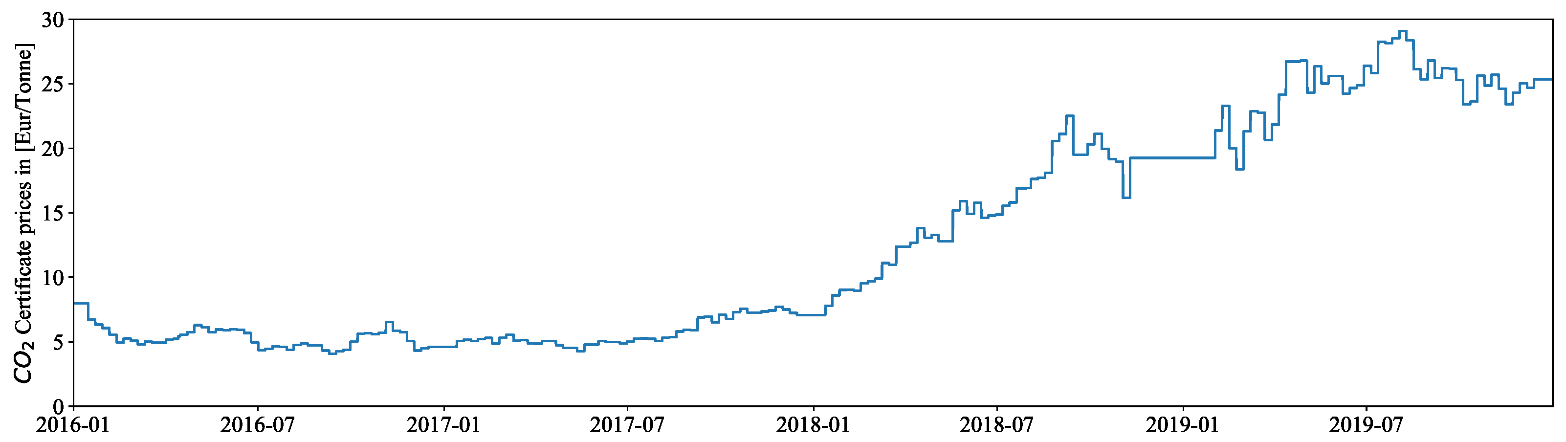
4.1.1. Fuel and CO Prices
4.1.2. Thermal Power Plant Parameters
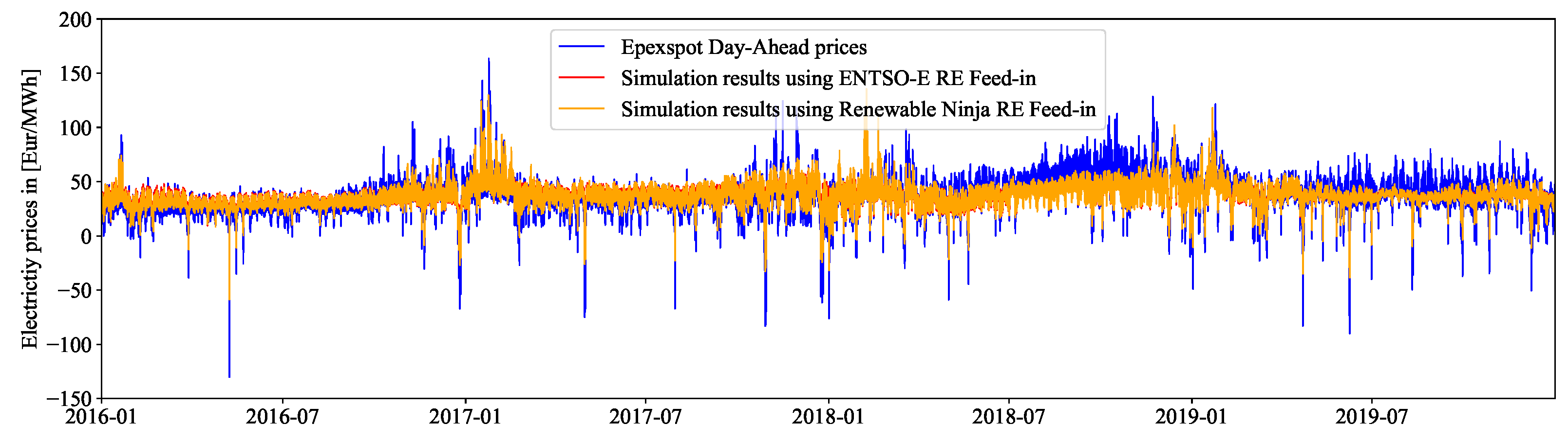
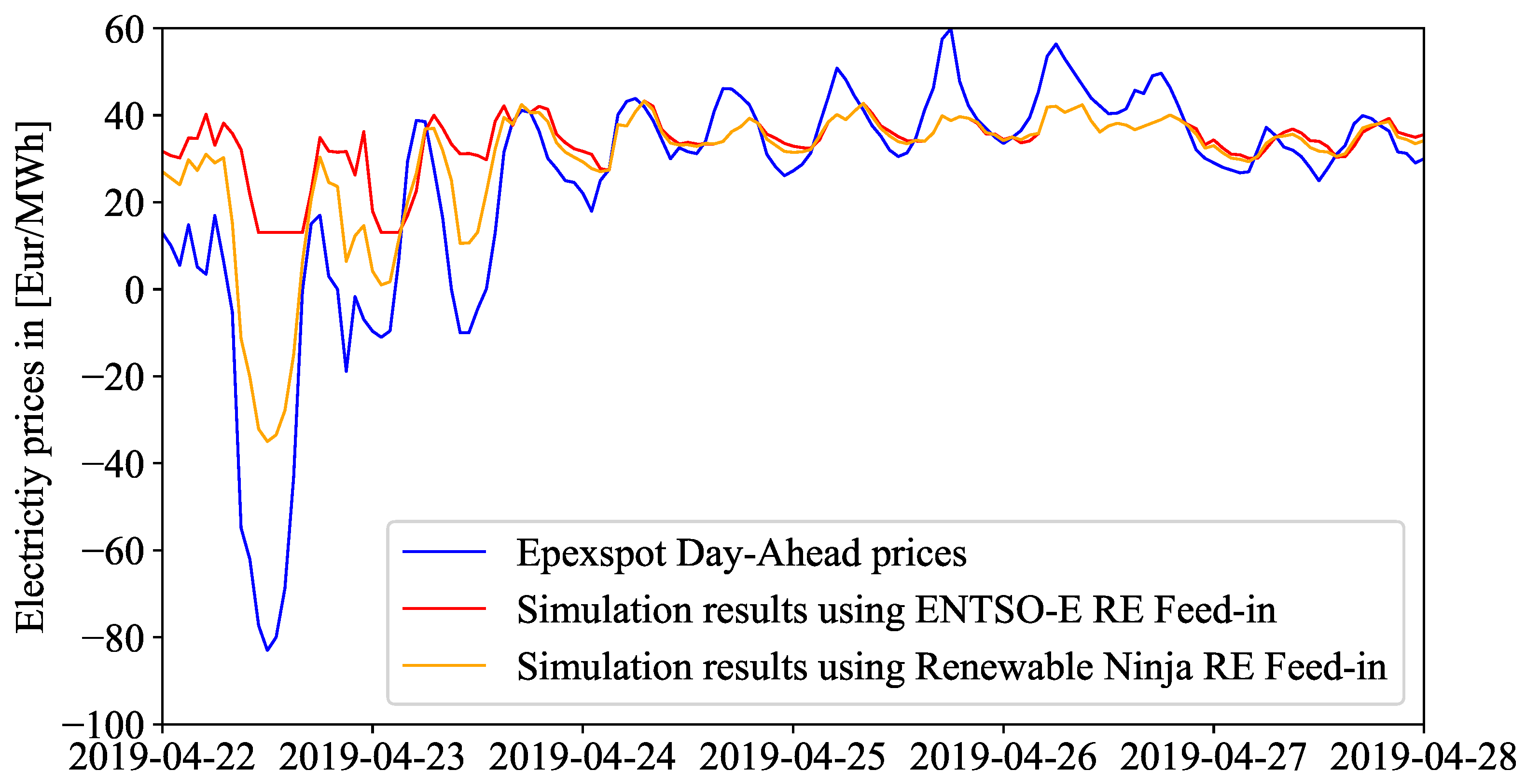
4.1.3. VRE Installed Capacities and Capacity Factors
4.1.4. Storage Units
4.1.5. Electricity and Control Reserve Demand
4.1.6. Heat Demand
4.1.7. Cross-Border Exchange
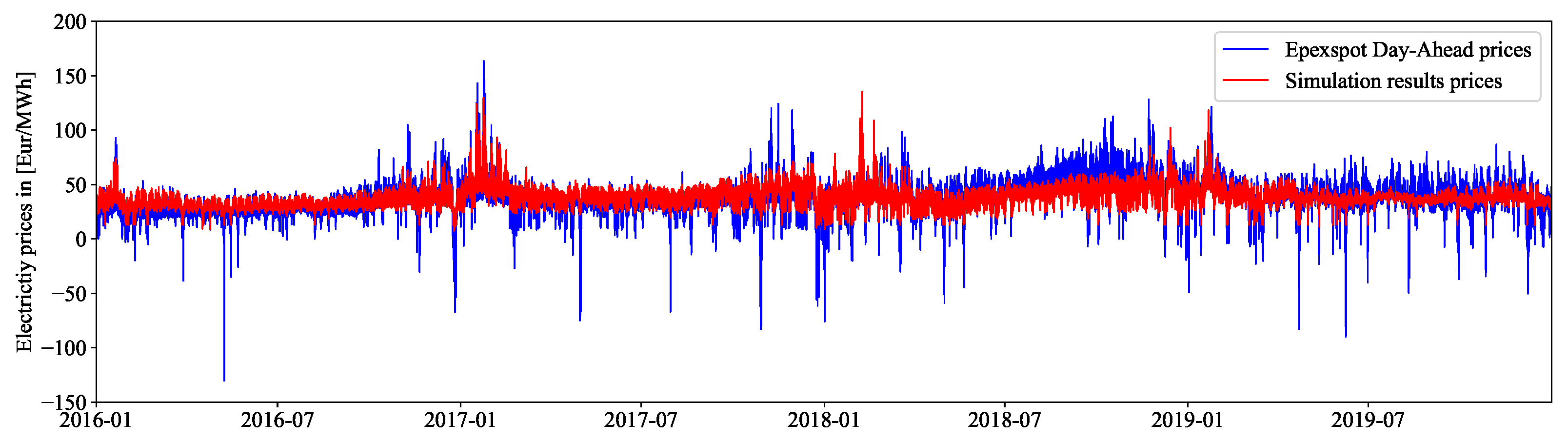
4.2. Modeled Prices and Generation Profiles
5. Conclusions and Outlook
Author Contributions
Funding
Data Availability Statement
Acknowledgments
Conflicts of Interest
Nomenclature
| Abbreviation | Description |
| EOM | Energy-only market |
| CRM | Control reserve market |
| DHM | District heating market |
| FERC | U.S. Federal Energy Regulatory Commission |
| LP | Linear problem |
| SFE | Supply function equilibrium |
| GPL | General Public License |
| GenCo | Generation company |
| OPF | Optimal power flow |
| UBA | German environment agency |
| BNetzA | German federal network regulation agency |
| VRE | Variable renewable energy |
| Symbols | Description |
| P | Power |
| PFC | Price forward curve |
| cm | Contribution margin |
| ep | Energy delivery price |
| cp | Capacity bid price |
| hp | Heat bid price |
| p | Fuel price |
| M | Market price |
| Power loss ratio | |
| Efficiency | |
| d | Average operation duration of the power plant |
| Subscripts | Description |
| t | Time interval in the EOM and DHM markets |
| Time interval in the CRM market | |
| theo | Theoritically available power |
| poss | Maximum possible power |
| ng | Natural gas |
| th | Thermal power delivered by the unit |
| el | Electrical power delivered by the unit |
| Superscripts | Description |
| hpp | Heat-power process |
| auxFi | Auxiliary firing |
| hp | Maximum possible heat extraction at the location |
| sd | Shut-down |
| su | Startup |
| inflex | Inflexible capacity |
| flex | Flexibile capacity |
| sup | Supply bid |
| dem | Demand bid |
| ES | Energy storage unit |
| TPP | Thermal power plant |
| pos | Positive reserve capacity/energy |
| neg | Negative reserve capacity/energy |
| max | Unit maximum technical capacity |
| min | Unit minimum technical capacity |
| ru | Ramp-up |
| rd | Ramp-down |
| con | Confirmed quantity |
References
- Joskow, P.L. Challenges for wholesale electricity markets with intermittent renewable generation at scale: The US experience. Oxf. Rev. Econ. Policy 2019, 35, 291–331. [Google Scholar] [CrossRef]
- Kell, A.; Forshaw, M.; McGough, A.S. ElecSim: Monte-Carlo Open-Source Agent-Based Model to Inform Policy for Long-Term Electricity Planning. In Proceedings of the Tenth ACM International Conference on Future Energy Systems, Phoenix, AZ, USA, 25–28 June 2019. [Google Scholar] [CrossRef]
- Weidlich, A.; Veit, D. A critical survey of agent-based wholesale electricity market models. Energy Econ. 2008, 30, 1728–1759. [Google Scholar] [CrossRef]
- Pfenninger, S.; Hawkes, A.; Keirstead, J. Energy systems modeling for twenty-first century energy challenges. Renew. Sustain. Energy Rev. 2014, 33, 74–86. [Google Scholar] [CrossRef]
- Ventosa, M.; Baíllo, Á.; Ramos, A.; Rivier, M. Electricity market modeling trends. Energy Policy 2005, 33, 897–913. [Google Scholar] [CrossRef]
- Boland, L. Equilibrium Models in Economics; Oxford University Press: New York, NY, USA, 2017. [Google Scholar] [CrossRef]
- Böhringer, C.; Rutherford, T. Combining Top-Down and Bottom-Up in Energy Policy Analysis: A Decomposition Approach. SSRN Electron. J. 2006. [Google Scholar] [CrossRef]
- Helgesen, P.I. Top-Down and Bottom-Up: Combining Energy System Models and Macroeconomic General Equilibrium Models: Working Paper; Norwegian University of Science and Technology: Trondheim, Norway, 2013. [Google Scholar]
- Ghersi, F. Hybrid Bottom-up/Top-down Energy and Economy Outlooks: A Review of IMACLIM-S Experiments. Front. Environ. Sci. 2015, 3, 74. [Google Scholar] [CrossRef]
- Hourcade, J.C.; Jaccard, M.; Bataille, C.; Ghersi, F. Hybrid Modeling: New Answers to Old Challenges Introduction to the Special Issue of The Energy Journal. Energy J. 2006, 27, 1–12. [Google Scholar] [CrossRef]
- European Commission. Joint Research Centre. Modelling Future EU Power Systems under High Shares of Renewables: The Dispa SET 2.1 Open Source Model; Joint Research Centre Publications Office: Ispra, Italy, 2017. [Google Scholar] [CrossRef]
- Leuthold, F.U.; Weigt, H.; von Hirschhausen, C. A Large-Scale Spatial Optimization Model of the European Electricity Market. Netw. Spat. Econ. 2012, 12, 75–107. [Google Scholar] [CrossRef]
- Brown, T.; Hörsch, J.; Schlachtberger, D. PyPSA: Python for Power System Analysis. J. Open Res. Softw. 2018, 6, 4. [Google Scholar] [CrossRef]
- Hilpert, S.; Kaldemeyer, C.; Krien, U.; Günther, S.; Wingenbach, C.; Plessmann, G. The Open Energy Modelling Framework (oemof)—A new approach to facilitate open science in energy system modelling. Energy Strategy Rev. 2018, 22, 16–25. [Google Scholar] [CrossRef]
- Hirth, L. The European Electricity Market Model EMMA Model Documentation; Neon Neue Energieökonomik GmbH: Berlin, Germany, 2017; pp. 1–17. [Google Scholar]
- Wiese, F.; Bökenkamp, G.; Wingenbach, C.; Hohmeyer, O. An open source energy system simulation model as an instrument for public participation in the development of strategies for a sustainable future. Wiley Interdiscip. Rev. Energy Environ. 2014, 3, 490–504. [Google Scholar] [CrossRef]
- Koch, M.; Bauknecht, D.; Heinemann, C.; Ritter, D.; Vogel, M.; Tröster, E. Modellgestützte Bewertung von Netzausbau im europäischen Netzverbund und Flexibilitätsoptionen im deutschen Stromsystem im Zeitraum 2020–2050. Z. Energiewirtschaft 2015, 39, 1–17. [Google Scholar] [CrossRef]
- Sun, N. Modellgestützte Untersuchung des Elektrizitätsmarktes: Kraftwerkseinsatzplanung und -Investitionen. Ph.D. Thesis, Universität Stuttgart, Stuttgart, Germany, 2013. [Google Scholar] [CrossRef]
- Gils, H.; Scholz, Y.; Pregger, T.; de Tena, D.L.; Heide, D. Integrated modelling of variable renewable energy-based power supply in Europe. Energy 2017, 123, 173–188. [Google Scholar] [CrossRef]
- Huppmann, D.; Egging, R. Market power, fuel substitution and infrastructure–A large-scale equilibrium model of global energy markets. Energy 2014, 75, 483–500. [Google Scholar] [CrossRef]
- Deissenroth, M.; Klein, M.; Nienhaus, K.; Reeg, M.; Varga, L. Assessing the Plurality of Actors and Policy Interactions: Agent-Based Modelling of Renewable Energy Market Integration. Complexity 2017, 2017, 7494313. [Google Scholar] [CrossRef]
- Abrell, J.; Kunz, F. Integrating Intermittent Renewable Wind Generation - A Stochastic Multi-Market Electricity Model for the European Electricity Market. Netw. Spat. Econ. 2015, 15, 117–147. [Google Scholar] [CrossRef]
- Gerbaulet, C.; Lorenz, C. dynELMOD: A Dynamic Investment and Dispatch Model for the Future European Electricity Market: Data Documentation; Deutsches Institut für Wirtschaftsforschung (DIW): Berlin, Germany, 2017. [Google Scholar]
- Kunz, F.; Zerrahn, A. Benefits of coordinating congestion management in electricity transmission networks: Theory and application to Germany. Util. Policy 2015, 37, 34–45. [Google Scholar] [CrossRef]
- Orgaz, A.; Bello, A.; Reneses, J. Multi-area electricity market equilibrium model and its application to the European case. In Proceedings of the 2017 14th International Conference on the European Energy Market (EEM), Dresden, Germany, 6–9 June 2017; pp. 1–6. [Google Scholar] [CrossRef]
- Liu, X.; Conejo, A.J. Single-Level Electricity Market Equilibrium with Offers and Bids in Energy and Price. IEEE Trans. Power Syst. 2021, 36, 4185–4193. [Google Scholar] [CrossRef]
- Gao, F.; Sheble, G. Electricity market equilibrium model with resource constraint and transmission congestion. Electr. Power Syst. Res. 2010, 80, 9–18. [Google Scholar] [CrossRef]
- Niu, H. Models for Electricity Market Efficiency and Bidding Strategy Analysis. Ph.D. Thesis, The University of Texas at Austin, Austin, TX, USA, 2005. [Google Scholar]
- Nitsch, F.; Schimeczek, C.; Frey, U.; Deissenroth-Uhrig, M.; Fuchs, B. FAME-Io. 2021. Available online: https://zenodo.org/record/4314338#.Yd0XD1kRXVg (accessed on 23 December 2021). [CrossRef]
- Cincotti, S.; Gallo, G. Gapex: An Agent-Based Framework for Power Exchange Modeling and Simulation. In Proceedings of the 4th International Conference on Agents and Artificial Intelligence, Algarve, Portugal, 6–8 February 2012; pp. 33–43. [Google Scholar] [CrossRef]
- Tesfatsion, L.; Battula, S. Analytical SCUC/SCED Optimization Formulation for AMES V5.0: ISU General Staff Papers; Iowa State University, Department of Economics: Ames, IA, USA, 2020. [Google Scholar]
- Andrade, R. A Multi-Agent System Simulation Model for Trusted Local Energy Markets. Master’s Thesis, Polytechnic of Porto—School of Engineering, Porto, Portogal, 2019. [Google Scholar]
- Conzelmann, G.; Boyd, G.; Koritarov, V.; Veselka, T. Multi-agent power market simulation using EMCAS. In Proceedings of the IEEE Power Engineering Society General Meeting, San Francisco, CA, USA, 16 June 2005; pp. 917–922. [Google Scholar] [CrossRef]
- Weidlich, A.; Sensfuß, F.; Genoese, M.; Veit, D. Studying the effects of CO2 emissions trading on the electricity market: A multi-agent-based approach. In Emissions Trading; Antes, R., Hansjürgens, B., Letmathe, P., Eds.; Springer: New York, NY, USA, 2008; pp. 91–101. [Google Scholar] [CrossRef]
- European Power Exchange SE–Epexspot. Trading Products; European Power Exchange: Paris, France, 2021. [Google Scholar]
- Borowski, P.F. Zonal and Nodal Models of Energy Market in European Union. Energies 2020, 13, 4182. [Google Scholar] [CrossRef]
- Abdel-Khalek, H.; Schäfer, M.; Vásquez, R.; Unnewehr, J.F.; Weidlich, A. Forecasting cross-border power transmission capacities in Central Western Europe using artificial neural networks. Energy Inform. 2019, 2, 12. [Google Scholar] [CrossRef]
- Weidlich, A.; Künzel, T.; Klumpp, F. Bidding Strategies for Flexible and Inflexible Generation in a Power Market Simulation Model: Model Description and Findings. In Proceedings of the Ninth International Conference on Future Energy Systems, Karlsruhe, Germany, 12–15 June 2018; Association for Computing Machinery: New York, NY, USA, 2018; pp. 532–537. [Google Scholar] [CrossRef]
- Schröder, A.; Kunz, F.; Meiss, J.; Mendelevitch, R.; Hirschhausen, C.V. Current and Prospective Costs of Electricity Generation Until 2050; DIW Data Documentation 68; Deutsches Institut für Wirtschaftsforschung (DIW): Berlin, Germany, 2013. [Google Scholar]
- Künzel, T. Entwicklung eines agentenbasierten Marktmodells zur Bewertung der Dynamik am deutschen Strommarkt in Zeiten eines steigenden Anteils erneuerbarer Energien. Ph.D. Thesis, KIT Scientific Publishing, Karlsruhe, Germany, 2019. [Google Scholar] [CrossRef]
- Konstantin, P. Praxisbuch Energiewirtschaft-Energieumwandlung, -Transport und -Beschaffung, Übertragungsnetzausbau und Kernenergieausstieg; Springer: Berlin/Heidelberg, Germany; New York, NY, USA, 2017. [Google Scholar]
- EEX. Market Data—EEX Group DataSource—Power—Natural Gas; EEX: Leipzig, Germany, 2019. [Google Scholar]
- EEX. Market Data—Environmental Markets—Auction Market; EEX: Leipzig, Germany, 2019. [Google Scholar]
- Statistische Bundesamt. Data on Energy Price Trends—Long-Time Series from January 2005 to June 2021; Statistische Bundesamt: Wiesbaden, Germany, 2021. [Google Scholar]
- S&P Global. World Electric Power Plants Database (WEPP); S&P Global: New York, NY, USA, 2016. [Google Scholar]
- Umwelt Bundesamt. Datenbank: Kraftwerke in Deutschland; Umwelt Bundesamt: Dessau-Rosslau, Germany, 2020. [Google Scholar]
- Bundesnetzagentur. BNetzA List of Power Plants; Bundesnetzagentur: Bonn, Germany, 2021. [Google Scholar]
- ENTSO-E. ENTSO-E Transparency Platform; ENTSO-E: Brussels, Belgium, 2021. [Google Scholar]
- SMARD Strommarktdaten. Available online: https://www.smard.de/en/downloadcenter/download-market-data (accessed on 15 April 2021).
- Pfenninger, S.; Staffell, I. Long-term patterns of European PV output using 30 years of validated hourly reanalysis and satellite data. Energy 2016, 114, 1251–1265. [Google Scholar] [CrossRef]
- Staffell, I.; Pfenninger, S. Using bias-corrected reanalysis to simulate current and future wind power output. Energy 2016, 114, 1224–1239. [Google Scholar] [CrossRef]
- Giesecke, J.; Mosonyi, E. Wasserkraftanlagen; Springer: Berlin/Heidelberg, Germany, 2009. [Google Scholar] [CrossRef]
- Arbeitsgemeinschaft Energiebilanzen e.V. Energie in Zahlen: Primärenergieverbrauch; Arbeitsgemeinschaft Energiebilanzen e.V.: Berlin, Germany, 2021. [Google Scholar]
- Deutscher Wetterdienst. Open Data area of the Climate Data Center; Deutscher Wetterdienst: Offenbach am Main, Germany, 2021. [Google Scholar]
- Grid Control Cooperation. Tender Overview and Results; Grid Control Cooperation. Available online: https://www.regelleistung.net/ext/tender/ (accessed on 15 April 2021).
- Koch, M.; Flachsbarth, F.; Bauknecht, D.; Heinemann, C.; Ritter, D.; Winger, C.; Timpe, C.; Gandor, M.; Klingenberg, T.; Tröschel, M. Dispatch of Flexibility Options, Grid Infrastructure and Integration of Renewable Energies Within a Decentralized Electricity System. In Advances in Energy System Optimization; Bertsch, V., Fichtner, W., Heuveline, V., Leibfried, T., Eds.; Springer International Publishing: Cham, Switzerland, 2017; pp. 67–86. [Google Scholar]
- Hellwig, M. Entwicklung und Anwendung Parametrisierter Standard-Lastprofile. Ph.D. Thesis, Technische Universität München, München, Germany, 2003. [Google Scholar]
- Genoese, F. Modellgestützte Bedarfs- und Wirtschaftlichkeitsanalyse von Energiespeichern zur Integration Erneuerbarer Energien in Deutschland; KIT Scientific Publishing: Karlsruhe, Germany, 2013. [Google Scholar] [CrossRef]
- Brand, H.; Weber, C.; Meibom, P.; Barth, R.; Swider, D. A stochastic energy. In Modelling in Energy Economics and Policy (CD-ROM); Swiss Federal Institute of Technology: Zürich, Switzerland, 2004. [Google Scholar]
- Möst, D.; Fichtner, W.; Rentz, O. Analysis of alpine hydropower with an optimising energy system model. In Proceedings of the ECOS 2005—The 18th International Conference on Efficiency, Cost, Optimization, Simulation, and Environmental Impact of Energy Systems, Trondheim, Norway, 20–22 June 2005; Tapir Academic Press: Trondheim, Norway, 2005; Volume 2, pp. 561–568. [Google Scholar]


| Model | Approach | Dispatch | Sectors | Spatial Resolution | Temporal Resolution | Reserves | Network | Open-Source | Reference |
|---|---|---|---|---|---|---|---|---|---|
| Dispa-Set | Optimization | Unit | Electricity, heat | Country | Hour | ✓ | Cross-border | ✓ | [11] |
| ELMOD | Optimization | Unit | Electricity, heat | Transmission network node | Hour | ✓ | DC-OPF | ✓ | [12] |
| PyPSA | Optimization | Unit | Cross-sectoral | Nodal | Hour | – | DC-OPF, LPF | ✓ | [13] |
| Oemof | Optimization | Unit | Cross-sectoral | Nodal | Hour | – | Transport model | ✓ | [14] |
| EMMA | Optimization | Type | Electricity | Country (North-Western Europe) | Hour | Minimum spinning reserve constraint | Cross-boder trades (ATC) | ✓ | [15] |
| Renpass | Optimization | Type | Electricity | Germany: 21 regions other countries: country | Hour | – | net transfer capacities | ✓ | [16] |
| PowerFlex | Optimization | Unit | Electricity, heat | Transmission network node | Hour | ✓ (as baseload) | DC-OPF | – | [17] |
| E2M2 | Optimization | Unit | Electricity, heat | Country | Hour | ✓ | – | – | [18] |
| REMix | Optimization | Type | Electricity, heat | Nodal | Hour | – | DC-OPF | – | [19] |
| AMIRIS | Simulation | Type | Electricity | Federal states (Germany) | 15 min | – | – | – | [20] |
| GAPEX | Simulation | Genco agents | Electricity | Power exchange markets | – | Net transfer capacities | – | [21] | |
| flexABLE | Simulation | Unit | Electricity, heat | Nodal | 15 min | ✓ | Linked to PyPSA | ✓ |
| Type | Data Description | Resolution Temporal, Spatial | Reference |
|---|---|---|---|
| Fuel and CO prices | Gas prices CO EU-ETS certificates Other energy carriers | 15 min, country-wise daily, country-wise 15 min, country-wise | [42] [43] [44] |
| Agents | Thermal power plants VRE power plants Storage units | -, unit-wise 15 min, country-wise -, unit-wise | [45,46,47] [48,49,50,51] [47,52] |
| Demand | Heat demand Weather data Inelastic demand Control reserve demand | 15 min, 16 regions hourly, 16 stations 15 min, 1 region 15 min, country-wise | [53] [54] [48] [55] |
| Imports and exports | Scheduled commercial exchanges | 15 min, country-wise | [48] |
| Simulation Period | MAE in €/MWh | RMSE in €/MWh |
|---|---|---|
| Year 2016 | 6.54 | 8.83 |
| Year 2017 | 9.44 | 13.01 |
| Year 2018 | 8.88 | 11.69 |
| Year 2019 | 6.69 | 10.91 |
| Total period | 7.89 | 11.21 |
Publisher’s Note: MDPI stays neutral with regard to jurisdictional claims in published maps and institutional affiliations. |
© 2022 by the authors. Licensee MDPI, Basel, Switzerland. This article is an open access article distributed under the terms and conditions of the Creative Commons Attribution (CC BY) license (https://creativecommons.org/licenses/by/4.0/).
Share and Cite
Qussous, R.; Harder, N.; Weidlich, A. Understanding Power Market Dynamics by Reflecting Market Interrelations and Flexibility-Oriented Bidding Strategies. Energies 2022, 15, 494. https://doi.org/10.3390/en15020494
Qussous R, Harder N, Weidlich A. Understanding Power Market Dynamics by Reflecting Market Interrelations and Flexibility-Oriented Bidding Strategies. Energies. 2022; 15(2):494. https://doi.org/10.3390/en15020494
Chicago/Turabian StyleQussous, Ramiz, Nick Harder, and Anke Weidlich. 2022. "Understanding Power Market Dynamics by Reflecting Market Interrelations and Flexibility-Oriented Bidding Strategies" Energies 15, no. 2: 494. https://doi.org/10.3390/en15020494
APA StyleQussous, R., Harder, N., & Weidlich, A. (2022). Understanding Power Market Dynamics by Reflecting Market Interrelations and Flexibility-Oriented Bidding Strategies. Energies, 15(2), 494. https://doi.org/10.3390/en15020494