Cost Efficient GPU Cluster Management for Training and Inference of Deep Learning

Abstract

Expanding the scale of GPU-based deep learning (DL) clusters would bring not only accelerated AI services but also significant energy consumption costs. In this paper, we propose a cost efficient deep learning job allocation (CE-DLA) approach minimizing the energy consumption cost for the DL cluster operation while guaranteeing the performance requirements of user requests. To do this, we first categorize the DL jobs into two classes: training jobs and inference jobs. Through the architecture-agnostic modeling, our CE-DLA approach is able to conduct the delicate mapping of heterogeneous DL jobs to GPU computing nodes. Second, we design the electricity price-aware DL job allocation so as to minimize the energy consumption cost of the cluster. We show that our approach efficiently avoids the peak-rate time slots of the GPU computing nodes by using the sophisticated mixed-integer nonlinear problem (MINLP) formulation. We additionally integrate the dynamic right-sizing (DRS) method with our CE-DLA approach, so as to minimize the energy consumption of idle nodes having no running job. In order to investigate the realistic behavior of our approach, we measure the actual output from the NVIDIA-based GPU devices with well-known deep neural network (DNN) models. Given the real trace data of the electricity price, we show that the CE-DLA approach outperforms the competitors in views of both the energy consumption cost and the performance for DL job processing.

1. Introduction

Recently, the Artificial Intelligence (AI) services based on deep learning (DL) have been dramatically expanded over the various area (e.g., image processing, computer vision, natural language processing, game learning, and self-driving system), while the non-negligible cost by the AI infrastructures have not been studied in detail yet. Most of the cost for DL application processing is caused from the energy consumption for GPU-based cluster operation [1]. For example, the maximum thermal design power (TDP) of state-of-the-art Ampere-based A100 GPU device (7 nm) is 400 W, which is higher than the older architecture of Volta-based V100 (12 nm, TDP-300 W) [2]. Generally, the GPU computing nodes in DL clusters, bring two types of energy consumption: idle energy consumption and active energy consumption [3]. The idle energy consumption is occurred when the node is turned on but has no running DL jobs. The active energy consumption is required when the node executes the assigned DL job. The active energy consumption is determined based on both the characteristics of the DL jobs (i.e., the number of deep neural network (DNN) model parameters and the input data size) and the hardware specification of the deployed GPU devices (i.e., the number of multi-processing units and core/memory clock rate) in the node [4]. Due to the complex mixture of such factors, the unsophisticated DL job allocation might bring the undesirable energy consumption cost for the cluster operation.

In order to reduce the energy consumption of the cluster operation, lots of studies have been presented so far. For reducing the energy consumption and carbon emission by clusters, refs. [5,6,7,8,9] have proposed the related approaches. Ghamkhari, M. et al. [5] propose the energy portfolio optimization for data center management. They present the linear mixed-integer stochastic programming approach with considering both the Internet workload data and the electricity market. They utilize the comprehensive energy options to maximize the energy efficiency of the cluster operation. Kwon, S. [6] proposes the renewable energy utilization based approach in order to achieve the energy efficient data center operations. The author designs the two-stage stochastic program with chance constraints to solve the energy usage optimization of clusters. Han, Z. et al. [7] propose the dynamic virtual machine (VM) management approach for energy efficient data centers. They formulate the large-scale Markov decision process (MDP) based problem to derive the energy-optimal decision making of VM allocation. They exploit the real trace data of user requests from the Google Cluster and PlanetLab to evaluate the practicality of their proposed approach. Hu, Q. et al. [8] propose the historical data based scheduling for DL workloads so as to improve the processing performance and achieve the sufficient energy saving. They design a Quasi-Shortest-Service-First scheduling approach in order to reduce the entire job completion time. Wang, Y. et al. [9] present sBEET that is the real-time energy efficient GPU scheduler, to maximize the performance of multitasking and achieve the energy optimization. They show the performance improvement by their proposed approach on the modern embedded GPU devices (e.g., NVIDIA Jetson Xavier AGX).

For energy efficient GPU-based cluster operation, refs. [10,11,12,13,14] have proposed the dynamic voltage and frequency scaling (DVFS)-based optimization techniques. Mei, X. et al. [10] propose the energy efficient online job scheduling on GPU-based clusters. They exploit the DVFS method so as to tune the energy efficient setting for GPU core/memory frequency values, according to the characteristics of the batch jobs. Guan, H. et al. [11] propose the virtual machine (VM) control architecture to achieve the energy-efficient SLA guarantees for cloud gaming in GPU-based clusters. They design the proportional-integral (PI) controller to adjust the GPU frequency for energy reduction. Zou, P. et al. [12] propose the quality of service (QoS) aware dynamic power management for GPU-based clusters by using the DVFS method. They present the online dynamic power-performance management (ODPP) system to maximize the energy efficiency given machine learning (ML) workloads. Bharadwaj, S. et al. [13] propose the DVFS-based technique, dynamic underclocking and bypassing (DUB) to enable the performance tuning for heterogeneous GPU workloads (bandwidth-intensive and latency-intensive), and achieve the power saving. Kandiah, V. et al. [14] design the power models for modern GPU device architectures based on various data including DVFS. They propose an AccelWattch, the configurable power modeling framework which is suitable for cluster environments consist of heterogeneous GPU devices.

Recently, modern DL based approaches have been proposed to maximize the energy efficiency of clusters. Ran, Y. et al. [15] propose the deep reinforcement learning (DRL) approach to achieve the joint optimization of job allocation and the data center cooling control. Instead of the conventional optimization methods, they present the parameterized deep Q-network (PADQN) to solve the control complexity of cluster operation. Gao, J. [16] proposes the neural network framework that leverages the multiple sensor data so as to estimate the data center performance and improve the associated energy efficiency. The proposed framework achieves the power usage effectiveness (PUE) of almost 1.1, for modern data centers. Wang, B. et al. [17] propose the DRL model-based QoS feature learning approach in order to decrease the energy consumption of cloud data centers while guaranteeing the low service-level-agreement (SLA) violation rate. Chi, C. et al. [18] present the model-free DRL based joint optimization method instead of using conventional optimization techniques, so as to achieve the data center energy optimization with the acceptable computation complexity.

However, even though existing works show the impressive results, the studies of the explicit energy efficient GPU-based cluster operation for DL job processing are still at an early stage. They have following several drawbacks.

First, they do not consider the heterogeneity of DL jobs. Without loss of generality, we can categorize the usual DL jobs into two classes: training jobs and inference jobs [19]. The DL training jobs require both of the feed-forward and back-propagation computations for DNN model parameter updating. The back-propagation computation needs longer duration than the feed-forward computation because of the diffusion of the chained gradient calculation. Usually, the DL training jobs require hours or days to get the acceptable estimation accuracy from the constructed DNN model. The DL training job is kind of batch workload, so we should pre-define the deadline for each DL training job. As long as satisfying the deadline, we are able to freely halt and restart the DL training jobs. The DL inference jobs require only the feed-forward computation for DNN model estimation. Contrast to the DL training jobs, the inference jobs require only few milliseconds or seconds to be completed. The DL inference job is kind of transactional workload, and the involved performance metric is the response latency which is commonly used for service quality evaluation. Consequently, the clusters handling DL training and inference jobs should do double duty like as the high performance computing (HPC) cluster for scientific applications and the data center (DC) for Internet workloads.

Second, the previous studies do not consider the heterogeneity of GPU device architectures. Generally, the deployed multiple GPU devices in clusters have different architectures due to the continuous upgrade [20]. The different GPU devices have the different computing capacity and derive the different power usage. In this case, it is not easy to design the common bottom-up model that is applicable for various GPU device architectures in general. Therefore, we need to design the generalized statistical models to estimate the GPU device power usage and the DL job performance, instead of using the certain model dedicated to the specific GPU architecture. Finally, the previous studies for GPU-based cluster operation do not consider the dynamic electricity price of the grid market. They commonly focus on only the training acceleration and the estimation accuracy, but not the electricity price-aware DL job allocation. Even with the same amount of energy consumption, the actual energy consumption cost for DL job processing may differ according to the variation of the electricity price [21]. For example, the energy consumption cost of the DL training job during the day-time may be higher than the one during the early hours of the morning.

In this paper, we propose a novel approach of cost efficient deep learning job allocation (CE-DLA), that minimizes the energy consumption cost of GPU-based cluster operation with DL job processing while guaranteeing the performance requirements of user requests. To do this, we categorize all the DL jobs into two classes of training and inference jobs, and formulate the deadline and the response latency as performance metrics. Our proposed CE-DLA approach is able to cover the allocation for heterogeneous DL jobs on the cluster. Furthermore, we exploit the statistical modeling approach to accommodate the heterogeneous GPU computing nodes in the cluster. Regardless of the GPU architecture diversity, our approach can be applied to common GPU-based clusters with DL job processing. Furthermore, we consider the dynamic electricity price of the grid market to reduce the energy consumption cost for cluster operation in practice. We conduct the DL job allocation with fine-granularity (i.e., time slot based delicate allocation) in the light of the electricity price variation, so as to enable the additional cost reduction even for the same energy consumption. The contributions of this work are as follows:

• To the best of our knowledge, this paper is the first work that conducts electricity price-aware allocation for both the DL training and inference jobs on the GPU-based cluster. Corresponding to the variation of the grid market price, our proposed approach automatically derives the cost optimal DL job allocation given workloads of user requests.
• The statistical power and performance models used in our formulation can be applied to general GPU-based clusters consist of heterogeneous GPU devices. At the cost of negligible estimation error, our approach efficiently estimates the GPU device power usage and the running DL job performance without the entire profiling of various GPU architectures.
• In order to reduce the energy consumption of idle GPU computing nodes, we exploit the dynamic right-sizing (DRS) method that temporarily turns the nodes having no DL jobs off. When the workloads of user requests are low, we can achieve the maximum cost efficiency via the DRS method.
• Through the sophisticated mixed integer nonlinear problem (MINLP) formulation, our approach easily finds the optimal solution considering all the aspects presented above.
• We exploit real trace data of GPU computing nodes and the grid market price, so as to establish the practical simulation experimental environments.

In order to evaluate the performance of our work practically, we first extract the real output data from the actual GPU computing nodes and the well-known DNN models. We deployed four types of GPU devices: GTX1060 (3 GB), GTX1060 (6 GB), 1080 (8 GB), and RTX2060 (6 GB) [2]. For DNN models, we exploit ResNet152 [22], VGG19Net [23], and InceptionV3 [24]. For input raw data, we exploit the ImageNet as the large-scale dataset [25]. Based on the framework of MS Computation Network Toolkit (CNTK) [26], we develop the Windows Powershell-based scripts to parse the output from the DL job processing. Second, we exploit the real trace data of dynamic electricity price from the Federal Energy Regulatory Commission (FERC) [27]. By using all the retrieved real data, we establish the practical simulation environment and conduct the various experiments. We demonstrate that our proposed CE-DLA approach outperforms other competitors for GPU-based cluster operation in views of energy consumption cost and the performance for DL job processing.

2. Main

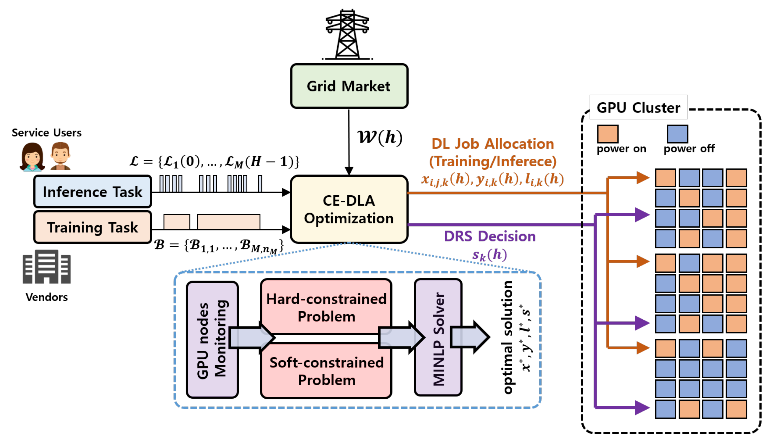
2.1. Proposed System Structure

Figure 1 shows the system structure with our proposed cost efficient deep learning allocation (CE-DLA) approach. The public service users and vendors continuously send the requests of DL training ($\mathcal{B}$) and inference jobs ($\mathcal{L}$) to our system. The requests of the DL training jobs contain the specification of the target DNN model, the dataset, the number of epochs to be trained, and the deadline. The requests of the DL inference jobs contain the specification of the target DNN model, the (single) input data, and the bound of acceptable response latency. At the same time, our system retrieves the trajectories of electricity price $\mathcal{W}$ from the grid market. In the work, we consider only the real-time electricity price, not the day-ahead one. Based on $\mathcal{B}$, $\mathcal{L}$, and $\mathcal{W}$, the system conducts both the DL job allocation and the GPU-based cluster operation. We present the the allocation procedures as follows.

• Step 1: The system begins to calculate the allocation decisions x and $(y,l)$ for the DL training and inference jobs, respectively.
• Step 2: For DL training jobs, the system maps the partial epochs of the jobs to the multiple time slots of GPU computing nodes. Each DL training job requires the feed-forward and back-propagation computations. In the feed-forward computation, user input data is sequentially passed over the DNN model weight parameters, and the output is derived from the last layer in the DNN model. After that, in the back-propagation computation, the model gradients are derived layer by layer based on the loss function value. After the calculation of all the gradients is done based on the chain-rule, the DNN model parameters are updated. The system iteratively conducts these procedures for all the pre-defined epochs.
• Step 3: For DL inference jobs, the system carries out the load-balancing for the input workloads on the available GPU computing nodes. In contrast to DL training jobs, each DL inference job requires only the feed-forward computation. Therefore, the DL inference jobs can be handled immediately. The system takes the DL inference jobs as the base workloads, and allocates them into the time slots right after they arrived.
• Step 4: If DL training jobs are deferrable, the system tries to halt-and-resume the assigned training jobs with considering the variation of the electricity price, as long as the deadline is not violated.
• Step 5: The system derives the DRS decision s for the GPU computing nodes in the cluster. The system turns idle nodes that have no running jobs off until it needs to deploy more available time slots for workload increasing. The system circumspectly conducts the turning-on/turning-off for nodes because the power state transition requires the non-negligible overheads [28].

The system formulates the optimization problems in order to make sophisticated allocation and operation decisions. By using the data (i.e., power usage and DL job processing time) measured by the GPU node parser, the system constructs two optimization problems: hard-constrained and soft-constrained problems. In the hard-constrained problem, the system tightly tries to satisfy the requirements of deadline and response latency bound for DL training and inference jobs. In this case, if the available time slots of nodes are not enough to accommodate all the jobs, then the system simply rejects some of the requests. In the soft-constrained problem, the system just penalizes the violation of the deadline and the response latency bound. In this case, the system tries to find the optimal trade-off between the service quality of user requests and the financial benefit of the cluster owner. After the problem formulation, the MINLP solver finds the optimal solution $x^{*}$, $y^{*}$, $l^{*}$, $s^{*}$ given workloads and electricity prices. The system applies the derived optimal solution to the cluster. We assume that our system accurately predicts the requests of the DL jobs and the grid market electricity prices during the control horizon. The detailed forecasting methods and the associated prediction error are not presented in this paper, and we will study such issues in the future work.

2.2. Proposed System Model

The goal of our work is to derive the optimal decision for DL training job scheduling, DL inference job balancing and computing node right-sizing in order to achieve the cost-efficient GPU-based cluster. To formulate the optimization problems, we consider K GPU computing nodes, and M DNN models. Let h and H denote the index of the certain time slot and the length of control horizon, respectively. We assume that the duration for a single time slot is 15 min. The notations used in the work are summerized in

Table 1. Notations used in Formulation.

Notation	Description
$\mathcal{B}=\{{\mathcal{B}}_{1,1},\cdots ,{\mathcal{B}}_{M,n_M}\}$	set of DL training jobs
${\mathcal{B}}_{i,j}=\{{\mathcal{A}}_{i,j},{\mathcal{E}}_{i,j},{\mathcal{Q}}_{i,j}^T\}$	individual j-th DL training job of i-th DNN model
${\mathcal{A}}_{i,j}$	arrived time slot index of ${\mathcal{B}}_{i,j}$
${\mathcal{E}}_{i,j}$	total count of epochs required to be trained in ${\mathcal{B}}_{i,j}$
${\mathcal{Q}}_{i,j}^T$	deadline index for ${\mathcal{B}}_{i,j}$
$\mathcal{L}=\{{\mathcal{L}}_1\left(0\right),\cdots ,{\mathcal{L}}_M(H-1)\}$	set of DL inference jobs
${\mathcal{L}}_i\left(h\right)$	number of DL inference jobs of i-th DNN model arrived
	at time slot h
${\mathcal{Q}}_i^I$	response latency bound for i-th DNN model
$\delta$	duration for a single time slot
${\mu }_{i,j,k}^T$	training completion time per an epoch
${\mu }_{i,k}^I$	response latency
${\lambda }_{i,k}$	arrival rate of partial workloads
$p_{i,j,k}^T$	power consumption for DL training jobs
$p_{i,k}^I$	power consumption for DL inference jobs
$\alpha ,\mathcal{F}$	statistical model coefficients
$e_k$	energy consumption of k-th GPU computing node
$\mathcal{W}\left(h\right)$	electricity price by grid market at time slot h
${\mathcal{O}}_{i,j,k}^{\mathrm{hr}},{\mathcal{O}}_k^{\mathrm{drs}}$	switching cost
${\mathcal{O}}^{\mathrm{T}},{\mathcal{O}}^I$	additional penalty cost for soft-constrained problem
$x_{i,j,k}\left(h\right)$	decision variable for DL training job allocation
$y_{i,k}\left(h\right)$	decision variable for DL inference job distribution
$l_{i,k}\left(h\right)$	decision variable for partial workloads in $L_i\left(h\right)$
	distributed to k-th GPU computing node
$s_k\left(h\right)$	decision variable for DRS method

.

2.2.1. Training and Inference Job Model

The characteristics of DL training and inference jobs are totally different. Generally, the number of invoked training jobs (e.g., tens to hundreds) is much less than the number of inference jobs during the day (e.g., ≈millions) [29]. The required processing time for DL training jobs is relatively long (i.e., hours to days) while the response latency of each DL inference job is very short (i.e., about milliseconds). Therefore the DL training jobs generally occupy multiple time slots to be completed while the DL inference jobs should be done within the allocated single time slot.

Let ${\mathcal{B}}_{i,j}$ denote the j-th training job for the i-th DNN model. Each job ${\mathcal{B}}_{i,j}$ involves the request specification $\{{\mathcal{A}}_{i,j},{\mathcal{E}}_{i,j},{\mathcal{Q}}_{i,j}^T\}$. The element ${\mathcal{A}}_{i,j}$ denotes the arrived time slot index of ${\mathcal{B}}_{i,j}$. The element ${\mathcal{E}}_{i,j}$ denotes the total number of epochs required to be trained in ${\mathcal{B}}_{i,j}$. The element ${\mathcal{Q}}_{i,j}^T$ denotes the time slot index of deadline for ${\mathcal{B}}_{i,j}$. Therefore, the number of remaining available time slots for ${\mathcal{B}}_{i,j}$ is ${\mathcal{Q}}_{i,j}^T-{\mathcal{A}}_{i,j}$. Let ${\mathcal{L}}_i\left(h\right)$ denote the number of DL inference jobs of i-th DNN model arrived at the time slot h, while the DL training job that is kind of a batch job considering the deadline, the DL inference job is in the category of transaction workload considering the response latency [30]. The upper-bound of acceptable response latency for DL inference jobs of i-th DNN model is defined as ${\mathcal{Q}}_i^I$. In the work, we assume that the response latency bound for DL inference jobs depends on the target DNN model type (i.e., the DL service type). That is, all the DL inference jobs of i-th DNN model have the same value ${\mathcal{Q}}_i^I$.

We define the request sets of DL training and inference jobs as follows:

$$\begin{array}{cc}\hfill \mathcal{B}& =\{{\mathcal{B}}_{1,1},{\mathcal{B}}_{1,2},\cdots ,{\mathcal{B}}_{1,n_1},{\mathcal{B}}_{2,1},{\mathcal{B}}_{2,2},\cdots ,{\mathcal{B}}_{2,n_2},\cdots ,{\mathcal{B}}_{M,n_M}\},\hfill \end{array}$$

(1)

$$\begin{array}{cc}\hfill \mathcal{L}& =\{{\mathcal{L}}_1\left(0\right),{\mathcal{L}}_2\left(0\right),\cdots ,{\mathcal{L}}_M\left(0\right),{\mathcal{L}}_1\left(1\right),{\mathcal{L}}_2\left(1\right),\cdots ,{\mathcal{L}}_M\left(1\right),\cdots ,{\mathcal{L}}_M(H-1)\}.\hfill \end{array}$$

(2)

Here, $n_i$ represents the number of invoked DL training jobs of i-th DNN model. From the viewpoint of the performance, for DL training jobs, the only thing we need to consider is the deadline compliance. This indicates that we are able to conduct the flexible scheduling for DL training jobs as long as the deadline is not violated. We freely postpone the partial epochs of the DL training jobs within the deadline. Meanwhile, for DL inference jobs, we should consider the short-term response latency, not the long-term deadline. Obviously, we cannot conduct the flexible scheduling approach for DL inference jobs due to the requirement of prompt execution. All the DL inference jobs should be done within their arrived time slots. In this case, we may regard DL inference jobs as the base workloads in each time slot.

2.2.2. Performance Model

The processing performance of DL training and inference jobs is affected by two factors: the characteristics of the assigned GPU device and the size of DNN model. The compute capability of processing units, core and memory clock rates, and the memory bandwidth of GPU device may affect the processing time of DL jobs [4]. Note that the GPU architectures deployed in modern clusters are commonly heterogeneous [20], and the processing time of DL jobs might be different according to the allocated GPU device types. Generally, it is not easy to establish the general bottom-up performance model for various commercial GPU devices. Instead, we exploit the statistical model to estimate the processing time of DL jobs allocated to heterogeneous GPU devices [31].

Let ${\mu }_{i,j,k}^T$ denote the training completion time per an epoch for j-th DL training jobs of i-th DNN model allocated to k-th GPU computing node. Then, the number of train-completed epochs per a time unit (i.e., a minute) is the reciprocal of ${\mu }_{i,j,k}^T$. Let $\delta$ denote the duration for a single time slot (i.e., 15 min). Then, the number of train-completed epochs during a time slot is calculated as follows:

$$\begin{array}{c}\hfill \frac{\delta }{{\mu }_{i,j,k}^T},\forall i,j,k.\end{array}$$

(3)

Let ${\mu }_{i,k}^I$ denote the service rate for DL inference jobs of i-th DNN model allocated to k-th computing GPU node. We assume that the probability that the GPU computing node is busy, is always 1 [32]. Then, we can derive the average response latency as follows:

$$\begin{array}{c}\hfill \frac{1}{{\mu }_{i,k}^I-{\lambda }_{i,k}}+\frac{1}{{\mu }_{i,k}^I},\forall i,k.\end{array}$$

(4)

where ${\lambda }_{i,k}$ represents the arrival rate of partial workloads in ${\mathcal{L}}_i$, distributed to k-th GPU computing node. Let $l_{i,k}$ denote the amount of partial workloads in ${\mathcal{L}}_i$, distributed to k-th GPU computing node by the load-balancing decision of our CE-DLA approach. Then, the arrival rate ${\lambda }_{i,k}$ can be derived as follows:

$$\begin{array}{c}\hfill {\lambda }_{i,k}=\frac{l_{i,k}}{\delta },\forall i,k.\end{array}$$

(5)

Obviously, we can exploit Equations (3) and (4) to construct the DL job performance constraints. We present the details in Section 2.2.6.

2.2.3. Power Consumption Model

If the GPU computing node is powered-on state and it is active, then its power consumption is proportional to the load of the running DL jobs. Let $p_{i,j,k}^T$ denote the power consumption for j-th DL training job of i-th DNN model allocated to k-th GPU computing node. The constants ${\alpha }_{i,j,k,1}^T$ and ${\alpha }_{i,j,k,2}^T$ represent the power model coefficients to derive $p_{i,j,k}^T$, respectively. They can be estimated the statistical modeling approach such as recursive least square (RLS) method [33]. Then we can derive the power consumption $p_{i,j,k}^T$ at time step h as follows:

$$\begin{array}{c}\hfill p_{i,j,k}^T\left(h\right)=\left\{\begin{array}{cc}{\alpha }_{i,j,k,1}^T{\mathcal{F}}_k+{\alpha }_{i,j,k,2}^T,\hfill & \mathrm{if}{x}_{i,j,k}\left(h\right)=1\hfill \\ 0,\hfill & \mathrm{if}{x}_{i,j,k}\left(h\right)=0\hfill \end{array}\right.\end{array}$$

(6)

where ${\mathcal{F}}_k$ is the performance factor of k-th GPU computing node. We set this value by including the compute capability and the clock rate of the GPU device. Here, $x_{i,j,k}\left(h\right)$ is the decision variable indicates whether the partial epochs of the DL training job ${\mathcal{B}}_{i,j}$ is allocated to k-th GPU computing node at time slot h or not (i.e., allocated = 1, not allocated = 0).

For DL inference jobs, we design the power consumption model based on the utilization of processing units [34]. Let $p_{i,k}^I$ denote the power consumption for DL inference jobs of i-th DNN model distributed to k-th GPU computing node. Similar to Equation (6) above, ${\alpha }_{i,k,1}^I$, ${\alpha }_{i,k,2}^I$, ${\alpha }_{i,k,3}^I$, and ${\alpha }_{i,k,4}^I$ are associated power model coefficients to estimate $p_{i,k}^I$. Let $u_{i,k}$ denote the average utilization of k-th GPU computing node with the partial workloads of ${\mathcal{L}}_i$. Then we define the power consumption $p_{i,k}^I$ at time step h as follows:

$$\begin{array}{c}\hfill p_{i,k}^I\left(h\right)=\left\{\begin{array}{cc}{\alpha }_{i,k,1}^I{\mathcal{F}}_k{u}_{i,k}\left(h\right)+{\alpha }_{i,k,2}^I{\mathcal{F}}_k+{\alpha }_{i,k,3}^I{u}_{i,k}\left(h\right)+{\alpha }_{i,k,4}^I,\hfill & \mathrm{if}{l}_{i,k}\left(h\right)>0,\hfill \\ 0,\hfill & \mathrm{if}{l}_{i,k}\left(h\right)=0,\hfill \end{array}\right.\end{array}$$

(7)

where $l_{i,k}\left(h\right)$ is the amount of partial workloads in ${\mathcal{L}}_i\left(h\right)$, distributed to k-th GPU computing node at time step h.

We can reformulate the average utilization of the node $u_{i,k}\left(h\right)$ as follows:

$$\begin{array}{c}\hfill u_{i,k}\left(h\right)=\frac{{\lambda }_{i,k}\left(h\right)}{{\mathcal{F}}_k},\forall i,k.\end{array}$$

(8)

Then, by integrating Equations (7) and (8), we can derive the reformulated power consumption model, in term of ${\lambda }_{i,k}$ as follows:

$$\begin{array}{c}\hfill p_{i,k}^I\left(h\right)=\left\{\begin{array}{cc}{\alpha }_{i,k,1}^I{\lambda }_{i,k}\left(h\right)+{\alpha }_{i,k,2}^I{\mathcal{F}}_k+{\alpha }_{i,k,3}^I\frac{{\lambda }_{i,k}\left(h\right)}{{\mathcal{F}}_k}+{\alpha }_{i,k,4}^I,\hfill & \mathrm{if}{l}_{i,k}\left(h\right)>0,\hfill \\ 0,\hfill & \mathrm{if}{l}_{i,k}\left(h\right)=0.\hfill \end{array}\right.\end{array}$$

(9)

Let $y_{i,k}\left(h\right)$ denote the indicator represents whether the DL inference jobs distributed to the GPU computing node or not. That is, $y_{i,k}\left(h\right)$ is defined as follows:

$$\begin{array}{c}\hfill y_{i,k}\left(h\right)=\left\{\begin{array}{cc}1,\hfill & \mathrm{if}{l}_{i,k}\left(h\right)>0,\hfill \\ 0,\hfill & \mathrm{if}{l}_{i,k}\left(h\right)=0.\hfill \end{array}\right.\end{array}$$

(10)

Based on Equations (5)–(10), we define the total power consumption of the k-th GPU computing node at time slot h as follows:

$$\begin{array}{cc}\hfill p_k\left(h\right)=& \sum _{\forall i}^{}\sum _{\forall j}^{}{x}_{i,j,k}\left(h\right)·({\alpha }_{i,j,k,1}^T{\mathcal{F}}_k+{\alpha }_{i,j,k,2}^T)\hfill \\ \hfill & +\sum _{\forall i}^{}{y}_{i,k}\left(h\right)·({\alpha }_{i,k,1}^I\frac{l_{i,k}\left(h\right)}{\delta }+{\alpha }_{i,k,2}^I{\mathcal{F}}_k+{\alpha }_{i,k,3}^I\frac{l_{i,k}\left(h\right)}{\delta ·{\mathcal{F}}_k}+{\alpha }_{i,k,4}^I)\hfill \\ \hfill & +p_k^{\mathrm{idle}},\forall k,h.\hfill \end{array}$$

(11)

where $p_k^{\mathrm{idle}}$ is the static power consumption when the k-th GPU computing node has no DL jobs. Consequently, our proposed CE-DLA approach can tune the power consumption for GPU computing nodes by adjusting decision variables x, y, and l, based on Equation (11) above.

2.2.4. Energy Consumption Model

Now, we are able to derive the energy consumption model based on both the performance and the power model defined above. Let $e_k\left(h\right)$ denote the energy consumption of the k-th GPU computing node at time slot h. The power state variable $s_k\left(h\right)$ indicates whether the k-th node is powered-on or powered-off state at time slot h. The energy consumption $e_k\left(h\right)$ is formulated as follows:

$$\begin{array}{c}\hfill e_k\left(h\right)=s_k\left(h\right)·p_k\left(h\right)·\delta ,\forall k,h.\end{array}$$

(12)

If the GPU computing node goes into the powered-off state at time slot h ($s_k\left(h\right)=0$), then the involved static power consumption is 0 W. In this paper, we exploit the linear electricity pricing model for implementation simplicity. Let $\mathcal{W}\left(h\right)$ denote the electricity price presented by the grid market at time slot h. Then the energy consumption cost for the entire cluster at time slot h is defined as follows:

$$\begin{array}{c}\hfill c_k\left(h\right)=e_k\left(h\right)·\mathcal{W}\left(h\right),\forall k,h.\end{array}$$

(13)

Finally, the total energy consumption cost for the entire cluster during all the time slots $h=1,\cdots ,H$ is formulated as follows:

$$\begin{array}{c}\hfill c=\sum _{\forall k}^{}\sum _{\forall h}^{}{c}_k\left(h\right)\end{array}$$

(14)

In order to reduce the energy consumption cost of the cluster, the CE-DLA approach prefers to assign the partial epochs of DL training jobs to the time slots at which the electricity price is low. Owing to the fine-grained structure (i.e., consists of multiple short-term iterations), we freely halt and restart running DL training jobs on the nodes. Furthermore, for time slots at which the electricity price is high, we can temporarily turn some of idle GPU computing nodes off by using the DRS method, so as to avoid the unnecessary static power consumption.

Note that there are non-negligible overheads for conducting halting-and-restarting the DL training jobs and the turning the nodes on again. In next section, we present the undesirable state transition cost occurred by those controls.

2.2.5. State Transition Cost Model

The first state transition cost is occurred by the halting-and-restarting process for DL training jobs. When the stopped DL training jobs resume, the node re-activates the library of the GPU device, re-uploads the trained DNN model parameters to the GPU global memory and reads the input dataset from the disk again. The associated cost is simply defined as follows:

$$\begin{array}{c}\hfill \sum _{\forall i}^{}\sum _{\forall j}^{}\sum _{\forall k}^{}\sum _{\forall h}^{}{\mathcal{O}}_{i,j,k}^{\mathrm{hr}}·max(x_{i,j,k}\left(h\right)-x_{i,j,k}(h-1),0).\end{array}$$

(15)

Here, the constant ${\mathcal{O}}_{ijk}^{\mathrm{hr}}$ represents the pre-measured overhead price for restarting the halted DL training job. For implementation simplicity, we do not consider the DL training job migration between different GPU computing nodes. Nevertheless, it is easy to modify or extend the equation above if we want to allow the DL training job migration.

The second state transition cost is occurred by the switching of DRS process. Obviously, we may see the additional overheads when the GPU computing node transits to the powered-off state from the powered-on state. According to [28], the cost generally contains the additional power consumption cost, reboot time consuming cost, and the wear-and-tear cost. Similar to Equation (15), the associated cost is defined as follows:

$$\begin{array}{c}\hfill \sum _{\forall k}^{}\sum _{\forall h}^{}{\mathcal{O}}_k^{\mathrm{drs}}·max(s_k\left(h\right)-s_k(h-1),0),\end{array}$$

(16)

where the constant ${\mathcal{O}}_k^{\mathrm{drs}}$ represents the cost for turning the GPU computing node on. This value only depends on the characteristics of the node.

2.2.6. Constraints

This section introduces the involved constraints for our problem formulation. The defined decision variables are x, y, l and s. Note that x, y and s are binary variables. The constraints for binary decision variables are defined as follows:

$$x_{i,j,k}\left(h\right)\in \{0,1\},\forall i,j,k,h.$$

(17)

$$y_{i,k}\left(h\right)\in \{0,1\},\forall i,k,h.$$

(18)

$$s_k\left(h\right)\in \{0,1\},\forall k,h.$$

(19)

We present the additional constraints for allowable job allocation as follows:

$${\mathcal{A}}_{i,j}\le x_{i,j,k}\left(h\right)\le s_k\left(h\right),\forall i,j,k,h.$$

(20)

$$\sum _{\forall i}^{}\sum _{\forall j}^{}\sum _{\forall k}^{}{x}_{i,j,k}\left(h\right)=1,\forall h.$$

(21)

$$x_{i,j,k}\left(h\right)·l_{i,k}\left(h\right)=0,\forall i,j,k,h.$$

(22)

$$0\le l_{i,k}\left(h\right)\le {\mathcal{L}}_i\left(h\right),\forall i,k,h.$$

(23)

$$\sum _{\forall k}^{}{l}_{i,k}\left(h\right)={\mathcal{L}}_i\left(h\right),\forall i,h.$$

(24)

$$l_{i,k}\left(h\right)\le s_k\left(h\right)·{\mathcal{L}}_i\left(h\right),\forall i,k,h.$$

(25)

$$y_{i,k}\left(h\right)\le l_{i,k}\left(h\right),\forall i,k,h.$$

(26)

The constraints (20) imply two conditions. The arbitrary DL training job cannot be allocated to the node before it arrives at the node. Furthermore, the DL training and inference jobs cannot be allocated to the nodes that are powered-off state. The constraints (21) imply that the arbitrary DL training job should be allocated to the single GPU computing node. The DL training job cannot be executed without the assigned node and it cannot be executed on more than two nodes in parallel. The constraints (22) imply that the common single node cannot accommodate both of the DL training and inference jobs simultaneously. The constraints (23) imply that the partial workloads $l_{i,k}\left(h\right)$ cannot exceed the entire workloads $l_i\left(h\right)$. The constraints (24) imply that the total sum of partial workloads of the DL inference jobs should be matched to the amount of entire requests. The constraints (25) imply that the DL inference jobs cannot be distributed to the GPU computing nodes that are powered-off state. The constraints (26) imply that $y_{i,k}\left(h\right)=1$ only when $L_{i,k}\left(h\right)>0$.

We present the constraints for acceptable performance for DL job processing as follows:

$$\sum _{\forall h}^{}\sum _{\forall k}^{}{x}_{i,j,k}\left(h\right)·\frac{\delta }{{\mu }_{i,j,k}^T}\ge {\mathcal{E}}_{i,j},\forall i,j.$$

(27)

$$h·x_{i,j,k}\left(h\right)\le {\mathcal{Q}}_{i,j}^T,\forall i,j,k,h.$$

(28)

$${\mu }_{i,k}^I-{\lambda }_{i,k}^I\left(h\right)\ge \frac{{\mu }_{i,k}^I}{{\mathcal{Q}}_i^I·{\mu }_{i,k}^I-1},\forall i,k,h.$$

(29)

The constraints (27) imply that all the epochs of the DL training jobs should be able to be trained within the allocated time slots. The constraints (28) imply that the DL training jobs cannot be allocated to the time slots that are after the deadline. The constraints (29) imply that the response latency for the distributed DL inference jobs should be below than the upper bound ${\mathcal{Q}}^I$. Contrast to DL training jobs, the DL inference jobs are not allowed to be postponed to later time slots. By reformulating Equations (4), we can derive the constraints (29).

If there is no feasible solution that satisfies the constraints (27)–(29) due to lack of GPU computing nodes, then the hard-constrained problem formulated in next Section 2.2.7 is infeasible. In this case, we should reject some of requests. In order to mitigate this risk, we additionally formulate the soft-constraint problem in Section 2.2.8.

2.2.7. Hard Constrained Problem Formulation

Based on the model and constraints presented above, we formulate the problem with the hard constraints as follows:

Problem 1.

(Hard-constrained Problem)

$$\begin{array}{cc}\hfill \underset{x,y,l,s}{minimize}& \sum _{\forall k}^{}\sum _{\forall h}^{}{c}_k\left(h\right)+\sum _{\forall i}^{}\sum _{\forall j}^{}\sum _{\forall k}^{}\sum _{\forall h}^{}{\mathcal{O}}_{i,j,k}^{\mathrm{hr}}·max(x_{i,j,k}\left(h\right)-x_{i,j,k}(h-1),0)\hfill \\ \hfill & +\sum _{\forall k}^{}\sum _{\forall h}^{}{\mathcal{O}}_k^{\mathrm{drs}}·\max (s_k\left(h\right)-s_k(h-1),0)\hfill \\ \hfill \mathit{subject}\mathit{to}.& \left(17\right)–\left(29\right).\hfill \end{array}$$

The advantages of the hard-constrained Problem 1 is that we can tightly ensure the acceptable performance of the DL jobs. However, there are several drawbacks at the same time. First, we may miss the opportunity to find the trade-off between the cost and the performance. We are inevitable to reject the some of requests despite the slight violation of the deadline and the response latency bound. For example, the requested DL training job should be completed within 10 h and the estimated deadline violation is only 15 min but nevertheless the system may reject that request. Second, the defined deadline and the response latency bound are sometimes just recommendations, not critical constraints. In this case, the strict enforcement of the performance constraints rather cause the degradation of the service quality due to too frequent request rejection. To solve such issues, we present the additional soft-constrained problem formulation in next section.

2.2.8. Soft Constrained Problem Formulation

In the soft-constrained problem formulation, we convert the constraints (17)–(29) to the additional cost terms for the objective function. In this approach, we flexibly accommodate the violation of the deadline and the response latency bound. By scaling the size of the attached weight values, we are able to gradually adjust the acceptable level for the DL job processing performance. Additionally, we can increase the cluster owner’s benefit at the minor cost of the slight performance degradation, and reduce the undesirable frequent request rejection. We formulate the problem with the soft constraints as follows:

Problem 2.

(Soft-constrained Problem)

$$\begin{array}{cc}\hfill \underset{x,y,l,s}{minimize}& \sum _{\forall k}^{}\sum _{\forall h}^{}{c}_k\left(h\right)+\sum _{\forall i}^{}\sum _{\forall j}^{}\sum _{\forall k}^{}\sum _{\forall h}^{}{\mathcal{O}}_{i,j,k}^{\mathrm{hr}}·max(x_{i,j,k}\left(h\right)-x_{i,j,k}(h-1),0)\hfill \\ \hfill & +\sum _{\forall k}^{}\sum _{\forall h}^{}{\mathcal{O}}_k^{\mathrm{drs}}·max(s_k\left(h\right)-s_k(h-1),0)\hfill \\ \hfill & +\sum _{\forall i}^{}\sum _{\forall j}^{}\sum _{\forall k}^{}\sum _{\forall h}^{}{\mathcal{O}}_{i,j,k}^{\mathrm{T}}·max(h·x_{i,j,k}\left(h\right)-{\mathcal{Q}}_{i,j}^T,0)\hfill \\ \hfill & +\sum _{\forall i}^{}\sum _{\forall k}^{}\sum _{\forall h}^{}{\mathcal{O}}_{i,k}^{\mathrm{I}}·max(\frac{{\mu }_{i,k}^I}{{\mathcal{Q}}_i^I·{\mu }_{i,k}^I-1}-\left({\mu }_{i,k}^I-{\lambda }_{i,k}^I\left(h\right)\right),0)\hfill \\ \hfill \mathit{subject}\mathit{to}.& \left(17\right)–\left(27\right).\hfill \end{array}$$

Here, ${\mathcal{O}}_{i,j,k}^{\mathrm{T}}$ and ${\mathcal{O}}_{i,k}^{\mathrm{I}}$ are the weight values for the violation of the deadline and the response latency bound, respectively. Note that if they are positive infinite values, then the soft-constrained Problem 2 is equivalent to the hard-constrained Problem 1. The max terms in the objective function can be converted to the linear forms. For details, see Appendix in [28]. In addition, the energy consumption model (i.e., Equation (12)) used in the problem formulation contains the product terms of decision variables x, y, l and s. We need to reformulate these terms in order to make the Problems 1 and 2 the convex ones. To do this, we can apply the exponential-transformation technique to the problem. For details, see [35].

2.2.9. Job Allocation Algorithm

The DL job allocation algorithm of the CE-DLA approach is presented in the Algorithm 1. The system receives the specifications of arrived DL training and inference job requests, and checks the involved parameters. According to the cluster operation policy, the system properly constructs the problem $\mathcal{P}$ (lines 01–05). If we want to ensure the acceptable performance of the DL job processing, then the system sets $\mathcal{P}$ as the hard-constrained problem (line 02). Otherwise, the system sets $\mathcal{P}$ as the soft-constrained problem (line 03). After then, the system checks the status of deployed CPU computing nodes in the cluster, and extracts the available time slots (line 06). If the feasible solution exists, then the system solve the problem $\mathcal{P}$ by using the MINLP solver (line 07). We exploit the well-known GUROBI optimizer to do this [36]. If the feasible solution does not exist, then the system rejects some of requests according to each priority value attached to the DL jobs (line 09). In this work, we do not present the details for establishing the priority policy. After the rejection, the system checks the feasibility of the problem $\mathcal{P}$ again (line 10). Finally, the system actuates the control for the cluster by using derived optimal solution $x^{*}$, $y^{*}$, $l^{*}$, and $s^{*}$.

Algorithm 1 DL Job Allocation based on the CE-DLA approach

INPUT: parameters $\alpha$, ${\mu }^T$, ${\mu }^I$, $\mathcal{W}$, H           request set of DL training jobs $\mathcal{B}=\{{\mathcal{B}}_{1,1},\cdots ,{\mathcal{B}}_{M,n_M}\}$           request set of DL inference jobs $\mathcal{L}=\{{\mathcal{L}}_1\left(0\right),\cdots ,{\mathcal{L}}_M(H-1)\}$           weight values ${\mathcal{O}}^{\mathrm{hr}}$, ${\mathcal{O}}^{\mathrm{drs}}$, ${\mathcal{O}}^{\mathrm{T}}$, ${\mathcal{O}}^{\mathrm{I}}$ OUTPUT: optimal solution ($x^{*}$, $y^{*}$, $l^{*}$, $s^{*}$) 01: ifEnsure acceptable performance then 02:  $\mathcal{P}⟵$ Hard-constrained Problem (1); 03: else if Find optimal trade-off then 04:  $\mathcal{P}⟵$ Soft-constrained Problem (2); 05: end if 06: if feasible solution exists in $\mathcal{P}$  then 07:   $x^{*}$, $y^{*}$, $l^{*}$, $s^{*}$ = solve $\mathcal{P}$ by using the MINLP solver [36]; 08:  else 09:   reject some of requests from $\mathcal{B}$ and $\mathcal{L}$ according to priorities; 10:   goto 06; 11: end if 12: actuate the cluster control by ($x^{*}$, $y^{*}$, $l^{*}$, $s^{*}$)

3. Experiments

For the experiments, we measure the actual data from our GPU devices, and the real trace data of the grid market electricity price. After then, we establish the simulation environment, so as to investigate the practical performance of our proposed CE-DLA approach compared to other competitors.

3.1. Experimental Setup

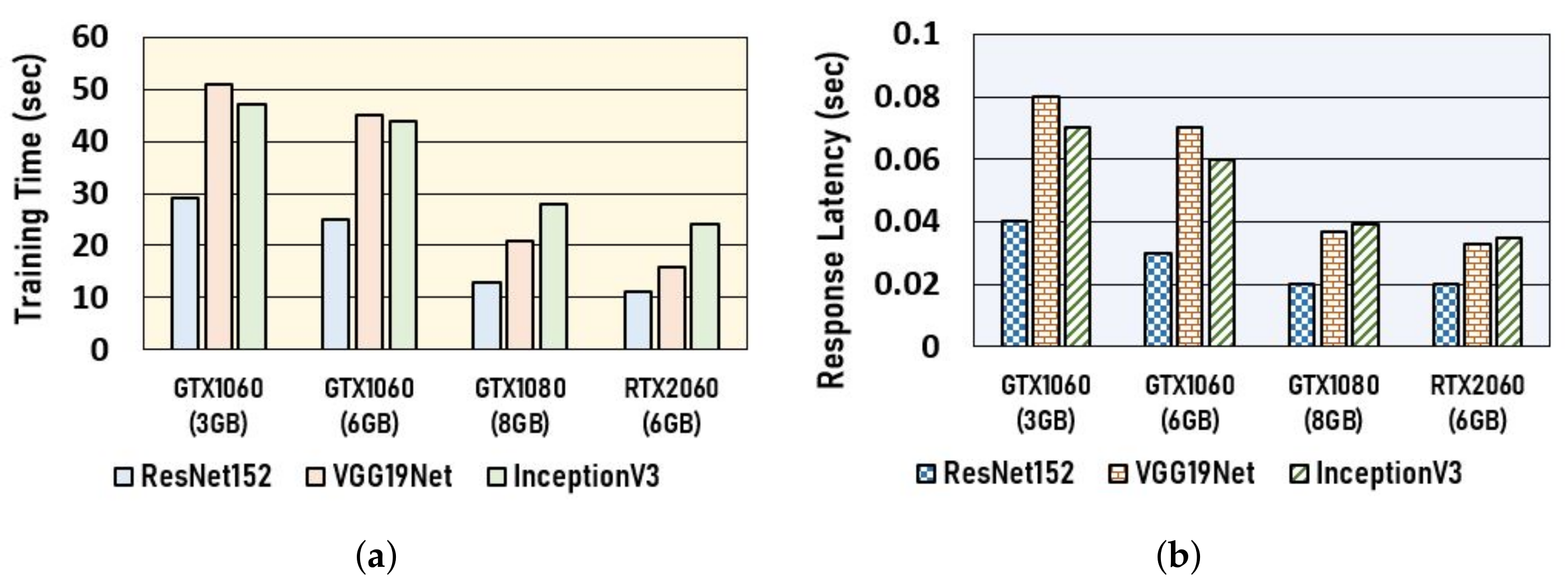
3.1.1. Deep Learning Job Setup

In order to establish the experimental testbed, we develop the Windows Powershell-based script codes by using the DL framework, MS Computation Network Toolkit (CNTK) [26]. For generating the DL training and inference jobs, we exploit three well-known DNN models: ResNet152 [22], VGG19Net [23], and InceptionV3 [24]. In this paper, for experimental simplicity, we only focus on the DL jobs for image processing. In order to construct the requests of the DL jobs, we exploit the open large-scale dataset [25]. We set the data batch size as 32 for each DL training job. For the DL inference job requests, we generate each request that contains the raw data of the single image. We develop the console-based output parser to collect the training time and the inference response latency from each DL job. All the codes are executed based on the Anaconda framework [37] that is the virtual environment with various python packages.

3.1.2. GPU Computing Node Setup

We measure the actual power and performance output from the real GPU computing nodes. We consider four types of the NVIDIA GPU devices: GTX1060 (3 GB), GTX1060 (6 GB), RTX2060 (6 GB), and the GTX1080 (8 GB) [2]. In order to measure the power consumption for each DL job, we use the utility, NVIDIA-SMI [38] that provides the monitoring data of the NVIDIA-based GPU device architectures. By using our implemented parser, we collect the power usage and the DL job processing time for each pair of GPU devices-DNN models. We exploit these actual data to establish our simulation environment. We assume that the average CPU utilization is always full (that is, almost 100%), and the involved power consumption of the CPU device is maximum during DL job processing.

3.1.3. Simulation Testbed Setup

Based on derived actual data from the GPU devices with three DNN models, we establish the practical simulation environment. We consider the cluster that contains 160 GPU computing nodes (i.e., GTX1060 (3 GB)-40 EA, GTX1060 (6 GB)-40EA, RTX2060 (6 GB)-40 EA, and GTX1080 (8 GB)-40 EA). For simplicity, we assume that the number of deployed GPU device within each node is only 1. The length of the entire horizon H is set as 7 days (i.e., $=168\left(\mathrm{h}\right)=\mathrm{10,080}\left(\min \right)=672(\mathrm{time}\mathrm{slots})$). Similar to the experimental setup of [4], the amount of DL training and inference jobs, and the involved deadline and the response latency, are generated by using the real job-trace and Gaussian distribution (avg = 50%, and std = 7.5% of possible shortest completion time/response latency).

We exploit the real trace data of the Federal Energy Regulatory Commission (FERC) [27] in order to draw the trajectory of the grid market electricity price. Especially, we use the locational based marginal price (LBMP) data ($/Wh) from the Syracuse power generator in New York Independent System Operator (NYISO) from 1 to 7 June 2018. Figure 2 shows the associated curve. We see that the regular pattern that the electricity price is high during the daytime (10 a.m.–6 p.m.) while it is low during the night.

3.1.4. Evaluation Metric

In order to evaluate our proposed CE-DCM system, we measure four metrics as follows:

(1) Deadline violation: For the DL training job ${\mathcal{B}}_{i,j}$, this performance metric is defined as $\mathit{m}\mathit{a}\mathit{x}({\overline{h}}_{i,j}^T-{\mathcal{Q}}_{i,j}^T,0)$ where ${\overline{h}}_{i,j}^T$ is the index of last allocated time slot to ${\mathcal{B}}_{i,j}$. The average deadline violation for all DL training jobs is defined as $\frac{{\sum }_{\forall i}^{}{\sum }_{j=0}^{n_i}\mathit{m}\mathit{a}\mathit{x}({\overline{h}}_{i,j}^T-{\mathcal{Q}}_{i,j}^T,0)}{{\sum }_{\forall i}^{}{n}_i}$. If we want to differentiate the priority of each DL training job, then we attach the weight parameters to the metric. Obviously, the ideal value of the deadline violation is 0.

(2) Latency bound violation: For the partial workloads of the DL inference job $l_{i,k}\left(h\right)$, this performance metric is defined as $l_{i,k}\left(h\right)·\mathit{m}\mathit{a}\mathit{x}({\mu }_{i,k}^I-{\lambda }_{i,k}^I\left(h\right)-\frac{{\mu }_{i,k}^I}{{\mathcal{Q}}_i^I·{\mu }_{i,k}^I-1},0)$. The average latency bound violation for all DL inference jobs is defined as

$\frac{{\sum }_{\forall i}{\sum }_{\forall k}{\sum }_{\forall h}{l}_{i,k}\left(h\right)·\mathit{m}\mathit{a}\mathit{x}({\mu }_{i,k}^I-{\lambda }_{i,k}^I\left(h\right)-\frac{{\mu }_{i,k}^I}{{\mathcal{Q}}_i^I·{\mu }_{i,k}^I-1},0)}{{\sum }_{\forall i}{\sum }_{\forall h}{\mathcal{L}}_i\left(h\right)}$. If we want to differentiate the priority of each DL inference job, then we attach the weight parameters to the metric. Similar to the deadline violation, the ideal value of the latency bound violation is also 0.

(3) Energy consumption: For the entire cluster, the total energy consumption is derived as ${\sum }_{\forall k}{\sum }_{\forall h}{e}_k\left(h\right)$.

(4) Energy consumption cost: For the entire cluster, the total energy consumption cost is derived as $c={\sum }_{\forall k}{\sum }_{\forall h}{e}_k\left(h\right)·\mathcal{W}\left(h\right)$. Note that the energy consumption cost is determined by both of the amount of energy consumption and the electricity price. Therefore the curve of energy consumption cost is not always same to the one of energy consumption. Obviously, the lower this value, the better the cost efficiency.

(5) Cost-to-performance ratio: For the entire cluster, the cost-to-performance ratio is defined as $\frac{(1-\mathrm{violation}\mathrm{ratio})\ast \#\mathrm{of}\mathrm{requests}}{c}$. This metric presents the number of DL (training and inference) jobs that we can ensure the involved performance requirements (deadline and latency bound), given the unit energy consumption cost (i.e., per 1 USD).

3.2. Competitors

We implement the existing approaches below, in order to compare them with our proposed CE-DLA approach.

(1) Baseline: This naive approach uses the first-input-first-output (FIFO) based job allocation for both the DL training and inference jobs. This approach does not consider the detailed job specification that contains the deadline and the response latency bound. For the implementation simplicity, we sometimes prefer to deploy this approach to the small-scale clusters. We exploit this approach to draw the worst bound of the derived performance and the cost to evaluate other approaches.

(2) EPRONS [39]: This approach proposes the job allocation for energy proportional network and server (EPRONS) in the cluster (e.g., data centers) by using the linear programming model. The authors focus on minimizing the energy consumption of latency-sensitive applications, i.e., DL inference jobs. This approach tries to find the optimal DRS decision while guaranteeing the response latency bound of the DL inference jobs. However, this approach does not consider the deadline-sensitive long-term applications, i.e., DL training jobs. In addition, the authors does not explicitly reflect the dynamic electricity price to the job allocation. In the EPRONS approach, we optimize $minN\ast P_{\mathrm{server}}\mathrm{s}.\mathrm{t}.K=K^{*}$, where N is the number of active (powered-on) servers, $P_{\mathrm{server}}$ is the amount of power consumption, and K is the scale factor ($K^{*}$ = optimal scale factor) for the latency-aware packet allocation. In this paper, we exploit $l_{i,k}$ as K to implement the EPRONS approach. In addition, we do not consider the cost for network links and switches defined in [39] in our model.

(3) PA-MBT [30]: The authors in this work present the performance aware allocation of mixed batch and transactional (PA-MBT) jobs, i.e., DL training and inference jobs. They propose the performance metric, relative performance functions (RPFs) to find the trade-offs between heterogeneous job requests. Their proposed method successfully achieves the acceptable deadline and response latency, however it does not consider the amount of energy consumption by each job and the associated electricity payment. Moreover, their approach cannot avoid the unnecessary energy consumption caused by the idle GPU computing nodes because of the absence of the DRS method. In the PA-MBT approach, we optimize $max{min}_m{u}_m\left(w_m\right)$ where m is the index of job, u is the RPF that measures the relative distance of the actual job processing time w from its requirement. The RPF value and the involved parameters can be determined based on the workload characteristics (i.e., training-batch or inference-transactional). In this paper, we exploit $\mu$ as w to implement the PA-MBT approach.

3.3. Evaluation

Figure 3 shows the DL job training time and inference latency according to our deployed GPU device types. Figure 3a shows the average completion time for training 10 iterations in an epoch of each pair of GPU devices-DNN models. Obviously, the GPU device, RTX2060 (6 GB) has the best performance (≈15 s in average) compared to other devices, due to its state-of-the-art architecture for parallel processing. Owing to the bigger memory size, the GTX1060 (6 GB) derives the better performance (≈36 s in average) than the GTX1060 (3 GB) (≈42 s in average) in spite of the same core architecture. Figure 3b shows the average response latency of DL inference jobs of each pair of GPU devices-DNN models. Similar to Figure 3a, the RTX2060 (6 GB) has the best performance for the latency (≈0.025 s in average) while the GTX1060 (3 GB) has the worst one (≈0.062 s in average). In view of the response latency, there is not a huge difference between the GTX1080 and RTX2060 because the feed-forward computation of the DL inference job is not heavy compared to the back-propagation computation. We exploit the data shown in Figure 3 to construct our simulation experiments.

Figure 4 compares the proposed CE-DLA approach with others in views of the violation of deadline and response latency bound. Figure 4a shows the average DL training job deadline violation (%) of the CE-DLA approach and others when the average DL inference job workload is (=${10}^5(\mathrm{reqs}/\min )$ (moderate)). The baseline approach has the worst result (≈7% at # of training jobs = 280) because it naively assigns the DL training jobs to time slots of the GPU computing nodes without consideration to the job specification. Except the baseline approach, the others derive the deadline violation about 2%, in average. This is because the total workload of the DL inference jobs is low, and the available time slots of the GPU computing nodes are enough to accommodate all the requests. Figure 4b shows the average DL training job deadline violation (%) when the average DL inference job workload is (=${17.5}^5(\mathrm{reqs}/\min )$ (high)). Due to the high workload of the DL inference job, the deadline violation of all the approaches is relatively large compared to Figure 4a. Especially, the EPRONS approach derives the deadline violation about (12% $\mathrm{at}\#\mathrm{of}\mathrm{training}\mathrm{jobs}=280$), and that result is worse than the PA-MBT and the CE-DLA approaches. This is because the EPRONS approach prefers to assign the DL jobs to the certain nodes that require the low energy consumption regardless of the compute capability. Similar to the CE-DLA approach, the PA-MBT approach shows the low deadline violation even at the high workload, because it finds the available earliest time slots of the nodes without considering the energy consumption. Figure 4c shows the average DL inference job latency violation (%) according to the workloads ($\mathrm{at}\#\mathrm{of}\mathrm{training}\mathrm{jobs}=175$ (moderate)). Obviously, when the workload of the DL inference jobs is low (=${10}^5(\mathrm{reqs}/\min )$), then the associated latency violation is not serious (≈2% in average) in all the approaches. Figure 4d shows the latency violation ($\mathrm{at}\#\mathrm{of}\mathrm{training}\mathrm{jobs}=280$ (high)). Similar to Figure 4b, the baseline and the EPRONS approaches derive the worse latency compared to the PA-MBT and the CE-DLA approaches, because they do not explicitly consider the performance of DL job processing. For all the cases, the PA-MBT approach shows the good performance compared to our proposed CE-DLA approach. Note that these results by the PA-MBT approach can be achieved at the non-negligble cost of the energy consumption.

Figure 5 compares the proposed CE-DLA approach with others in views of both the energy consumption and the energy consumption cost. The total energy consumption (kWh) occurred by the CE-DLA approach and the others when the average DL inference job workload is (=${10}^5(\mathrm{reqs}/\min )$), is shown in Figure 5a. The baseline approach derives the worst energy consumption about (3500 kWh $\mathrm{at}\#\mathrm{of}\mathrm{training}\mathrm{jobs}=280$) because it assigns the DL training jobs according to the arrival ordering, not the energy consumption. The EPRONS and our proposed CE-DLA approaches derive almost same the energy consumption (≈600 kWh in average) along all the cases, because both of them try to find the energy optimal time slots for the DL job allocation. Contrast to results of the performance in Figure 4, the PA-MBT approach has the worse energy consumption (≈1300 kWh in average) compared to the EPRONS and the CE-DLA approaches. The PA-MBT approach tries to properly balance both the batch (training) and transaction (inference) workloads with considering the heterogeneous performance requirements similar to our CE-DLA approach, however it does not consider the amount of the involved energy consumption. Figure 5b shows the energy consumption according to the DL inference job workloads ($\mathrm{at}\#\mathrm{of}\mathrm{training}\mathrm{jobs}=175$). Similar to Figure 5a, both the baseline and the PA-MBT approaches derive relatively the high energy consumption for DL job allocation compared to the EPRONS and the CE-DCM approaches. Figure 5c shows the energy consumption cost ($) for all the approaches when the average DL inference job workload is (=${10}^5(\mathrm{reqs}/\min )$), with the real trace data of the FERC. The bar shapes of the energy consumption cost in Figure 5c are similar to the ones in Figure 5a, however the EPRONS approach has the worse energy consumption cost compared to our proposed CE-DLA approach. This is because the EPRONS approach only considers the amount of energy consumption, not the grid market electricity price. As mentioned earlier, the energy consumption cost can be different even for the same amount of energy consumption by the variation of the electricity price. Our proposed CE-DLA approach directly reflects the dynamic electricity price to the DL job allocation, so as to minimize the energy consumption cost as shown in Figure 5c. Figure 4d shows the energy consumption cost according to the DL inference job workloads ($\mathrm{at}\#\mathrm{of}\mathrm{training}\mathrm{jobs}=175$). Concurrent with the results of Figure 5c, our proposed CE-DLA approach outperforms the competitors in view of the energy consumption cost.

Figure 6 compares the cost-to-performance ratio of all the methods. We can find that our proposed CE-DLA method outperforms other competitors in view of the cost efficiency. In Figure 6a, the soft-constrained modeling approach of the CE-DLA method achieves the cost-to-performance ratio (5.26/1 $) about 2.5 times of the ratio (2.09/1 $) of PA-MBT method. Although the cost-to-performance ratio of the hard-constrained modeling approach is slightly worse than the soft-constrained modeling approach, it still outperforms all of other competitors. In Figure 6, we also see the superiority of the CE-DLA method for DL inference jobs over others, similar to Figure 6a.

Table 2. The ratio of DL training job allocation on 3 pricing ranges [USD 0–20], [USD 20–30], and [USD 30–50].

	CE-DLA	EPRONS	PA-MBT
USD 0–20	0.59	0.31	0.28
USD 20–30	0.40	0.63	0.59
USD 30–50	0.01	0.09	0.13

shows the ratio of DL training job allocation of each method on three pricing ranges: [USD 0–20], [USD 20–30], and [USD 30–50]. Contrast to others, in the CE-DLA method, more than half of all the DL training jobs is allocated to the cheapest pricing range [USD 0–20]. Obviously, our proposed CE-DLA method outperforms other competitors (including EPRONS) in view of cost-efficiency. These results support the experimental results shown in Figure 5c,d.

Additionally, we try to investigate the rejection ratio of our proposed CE-DLA method when the workload is extremely high (400 training jobs, 2500 inference requests/min). For implementation simplicity, we assume that only the training jobs are rejected (the inference jobs are not).

Table 3. Number of rejected DL training jobs for workloads of (280 training jobs, 1700 inference reqs/min) and (400 training jobs, 2500 inference reqs/min).

	Soft-Constrained	Hard-Constrained	PA-MBT
280, 1700	3 jobs (1%)	9 jobs (3.2%)	9 jobs (3.2%)
400, 2500	45 jobs (11.2%)	98 jobs (24.5%)	97 jobs (24.2%)

shows the results. The hard-constrained modeling approach of the CE-DLA method derives the high rejection ratio (98 DL training jobs, 24.5%) similar to the PA-MBT (97 DL training jobs, 24.2%). In contrast, the soft-constrained modeling approach achieves the reduced rejection ratio (45 DL training jobs, 11.2%) with the slight violation of the performance requirement of DL jobs. If we set the weight constants ${\mathcal{O}}_{i,j,k}^{\mathrm{T}}$ and ${\mathcal{O}}_{i,j}^{\mathrm{I}}$ by large values, then the soft-constrained modeling approach may achieve the better cost efficiency than others, but it may also bring the undesirable performance degradation (by the violation allowance). Note that both the hard and soft-constrained modeling approaches derive the high rejection ratio when the workload is extremely high (400 training jobs/2500 inference reqs/min). If the workload is too high and the available nodes are lack to accommodate all the requests, then it is inevitable to reject a lot of requests regardless of the allocation algorithm design. Our proposed method achieves the financial benefit only when the workload is not too tight to process. We think that almost algorithms targeting to cost-efficient resource allocation, have the same issue. This problem is not from the weakness of the algorithm design, but from the lack of available resources. If we want to solve such issues, we should deploy more servers into the cluster.

4. Conclusions

In this paper, we propose the energy consumption cost efficient deep learning job allocation (CE-DLA) method for GPU-based cluster operation. To the best of our knowledge, this is the first work conducts the performance- and the cost-driven allocation for both the DL training and inference jobs given the dynamic electricity price. We design the mixed integer nonlinear programming (MINLP) formulation based on the statistical modeling which is not dedicated for certain GPU device architectures and DL jobs. We present the deferrable DL training job scheduling and integrate it with the dynamic right-sizing (DRS) method. Our sophisticated approach enables both the ensurance of the performance requirements (deadline and latency bound) and the energy consumption cost svaing for DL job processing. Through the large-scale simulation results based on real data of NVIDIA-based GPU cards and the execution profiling, we show that our method is practical for modern GPU-based clusters. The soft-constrained modeling approach of the CE-DLA method achieves the cost-to-performance ratio about 2 times on average, than previous performance-driven approach (PA-MBT) and energy-driven approach (EPRONS). In view of energy consumption cost, our CE-DLA method improves the cost saving of 29% than the competitors (43% than PA-MBT, and 15% than EPRONS) while guranteeing the acceptable performance. In future work, we will explore the cost-efficient framework covering the entire steps of DL jobs, i.e., including data preprocessing, data transmission between nodes in cluster, DNN model training/inferencing and the response submission to users.

References

1. Gawande, N.A.; Daily, J.A.; Siegel, C.; Tallent, N.R.; Vishnu, A. Scaling deep learning workloads: Nvidia dgx-1/pascal and intel knights landing. Future Gener. Comput. Syst. 2020, 108, 1162–1172. [Google Scholar] [CrossRef]
2. NVIDIA. Available online: https://www.nvidia.com/en-us/ (accessed on 6 December 2021).
3. Gu, C.; Li, Z.; Huang, H.; Jia, X. Energy efficient scheduling of servers with multi-sleep modes for cloud data center. IEEE Trans. Cloud Comput. 2018, 8, 833–846. [Google Scholar] [CrossRef]
4. Kang, D.K.; Ha, Y.G.; Peng, L.; Youn, C.H. Cooperative Distributed GPU Power Capping for Deep Learning Clusters. IEEE Trans. Ind. Electron. 2021. [Google Scholar] [CrossRef]
5. Ghamkhari, M.; Wierman, A.; Mohsenian-Rad, H. Energy portfolio optimization of data centers. IEEE Trans. Cloud Comput. 2016, 8, 1898–1910. [Google Scholar] [CrossRef]
6. Kwon, S. Ensuring renewable energy utilization with quality of service guarantee for energy-efficient data center operations. Appl. Energy 2020, 276, 115424. [Google Scholar] [CrossRef]
7. Han, Z.; Tan, H.; Wang, R.; Chen, G.; Li, Y.; Lau, F.C.M. Energy-efficient dynamic virtual machine management in data centers. IEEE/ACM Trans. Netw. 2019, 27, 344–360. [Google Scholar] [CrossRef]
8. Hu, Q.; Sun, P.; Yan, S.; Wen, Y.; Zhang, T. Characterization and Prediction of Deep Learning Workloads in Large-Scale GPU Datacenters. In Proceedings of the International Conference for High Performance Computing, Networking, Storage and Analysis (SC), St. Louis, MO, USA, 16–18 November 2021; pp. 1–15. [Google Scholar]
9. Wang, Y.; Karimi, M.; Xiang, Y.; Kim, H. Balancing Energy Efficiency and Real-Time Performance in GPU scheduling. In Proceedings of the 2021 IEEE Real-Time Systems Symposium (RTSS), Virtual Event, 7–10 December 2021; pp. 110–122. [Google Scholar]
10. Mei, X.; Chu, X.; Liu, H.; Leung, Y.W.; Li, Z. Energy efficient real-time task scheduling on CPU-GPU hybrid clusters. In Proceedings of the IEEE Conference on Computer Communications (INFOCOM), Atlanta, GA, USA, 1–4 May 2017; pp. 1–9. [Google Scholar]
11. Guan, H.; Yao, J.; Qi, Z.; Wang, R. Energy-efficient SLA guarantees for virtualized GPU in cloud gaming. IEEE Trans. Parallel Distrib. Syst. 2014, 26, 2434–2443. [Google Scholar] [CrossRef]
12. Zou, P.; Ang, L.P.; Barker, K.; Ge, R. Indicator-Directed Dynamic Power Management for Iterative Workloads on GPU-Accelerated Systems. In Proceedings of the 20th IEEE/ACM International Symposium on Cluster, Cloud and Internet Computing (CCGRID), Melbourne, Australia, 11–14 May 2020; pp. 559–568. [Google Scholar]
13. Bharadwaj, S.; Das, S.; Eckert, Y.; Oskin, M.; Krishna, T. DUB: Dynamic underclocking and bypassing in nocs for heterogeneous GPU workloads. In Proceedings of the 2021 15th IEEE/ACM International Symposium on Networks-on-Chip (NOCS), Virtual Event, 14–15 October 2021; pp. 49–54. [Google Scholar]
14. Kandiah, V.; Peverelle, S.; Khairy, M.; Pan, J.; Manjunath, A.; Rogers, T.G.; Aamodt, T.M.; Hardavellas, N. AccelWattch: A Power Modeling Framework for Modern GPUs. In Proceedings of the 54th Annual IEEE/ACM International Symposium on Microarchitecture (MICRO), Athens, Greece, 18–22 October 2021; pp. 738–753. [Google Scholar]
15. Ran, Y.; Hu, H.; Zhou, X.; Wen, Y. Deepee: Joint optimization of job scheduling and cooling control for data center energy efficiency using deep reinforcement learning. In Proceedings of the IEEE 39th International Conference on Distributed Computing Systems (ICDCS), Dallas, TX, USA, 7–9 July 2019; pp. 645–655. [Google Scholar]
16. Gao, J. Machine Learning Applications for Data Center Optimization (Google, 2014). Available online: https://research.google/pubs/pub42542/ (accessed on 6 December 2021).
17. Wang, B.; Liu, F.; Lin, W. Energy-efficient VM scheduling based on deep reinforcement learning. Elsevier Future Gener. Comput. Syst. 2021, 125, 616–628. [Google Scholar] [CrossRef]
18. Chi, C.; Ji, K.; Song, P.; Marahatta, A.; Zhang, S.; Zhang, F.; Qiu, D.; Liu, Z. Cooperatively Improving Data Center Energy Efficiency Based on Multi-Agent Deep Reinforcement Learning. Energies 2021, 14, 2071. [Google Scholar] [CrossRef]
19. Wu, S.; Li, G.; Chen, F.; Shi, L. Training and inference with integers in deep neural networks. arXiv 2018, arXiv:1802.04680. [Google Scholar]
20. Chaudhary, S.; Ramjee, R.; Sivathanu, M.; Kwatra, N.; Viswanatha, S. Balancing efficiency and fairness in heterogeneous GPU clusters for deep learning. In Proceedings of the Fifteenth European Conference on Computer Systems (EuroSys), Heraklion, Crete, Greece, 27–30 April 2020; pp. 1–16. [Google Scholar]
21. Wu, W.; Wang, W.; Fang, X.; Junzhou, L.; Vasilakos, A.V. Electricity price-aware consolidation algorithms for time-sensitive vm services in cloud systems. IEEE Trans. Serv. Comput. 2019. [Google Scholar] [CrossRef] [Green Version]
22. He, K.; Zhang, X.; Ren, S.; Sun, J. Deep residual learning for image recognition. In Proceedings of the IEEE Conference on Computer Vision and Pattern Recognition (CVPR), Las Vegas, NV, USA, 26 June–1 July 2016; pp. 770–778. [Google Scholar]
23. Simonyan, K.; Zisserman, A. Very deep convolutional networks for large-scale image recognition. In Proceedings of the Ninth International Conference on Learning Representations (ICLR), San Diego, CA, USA, 7–9 May 2015; pp. 770–778. [Google Scholar]
24. Szegedy, C.; Vanhoucke, V.; Ioffe, S.; Shlens, J.; Wojna, Z. Rethinking the inception architecture for computer vision. In Proceedings of the IEEE Conference on Computer Vision and Pattern Recognition (CVPR), Las Vegas, NV, USA, 26 June–1 July 2016; pp. 2818–2826. [Google Scholar]
25. Krizhevsky, A.; Sutskever, I.; Hinton, G.E. Imagenet classification with deep convolutional neural networks. In Proceedings of the Advances in Neural Information Processing Systems (NIPS), Lake Tahoe, NV, USA, 3–8 December 2012; Volume 25, pp. 1097–1105. [Google Scholar]
26. Microsoft Computation Network Toolkit (CNTK). Available online: https://github.com/Microsoft/CNTK (accessed on 6 December 2021).
27. Federal Energy Regulatory Commission (FERC). Available online: https://www.ferc.gov/ (accessed on 6 December 2021).
28. Lin, M.; Wierman, A.; Andrew, L.L.; Thereska, E. Dynamic right-sizing for power-proportional data centers. IEEE/ACM Trans. Netw. 2013, 21, 1378–1391. [Google Scholar] [CrossRef]
29. Wu, C.J.; Brooks, D.; Chen, K.; Chen, D.; Choudhury, S.; Dukhan, M.; Hazelwood, K.; Isaac, E.; Jia, Y.; Jia, B.; et al. Machine learning at facebook: Understanding inference at the edge. In Proceedings of the 2019 IEEE International Symposium on High Performance Computer Architecture (HPCA), Washington, DC, USA, 16–20 February 2019; pp. 331–344. [Google Scholar]
30. Carrera, D.; Steinder, M.; Whalley, I.; Torres, J.; Ayguade, E. Autonomic placement of mixed batch and transactional workloads. IEEE Trans. Parallel Distrib. Syst. 2012, 23, 219–231. [Google Scholar] [CrossRef]
31. Abe, Y.; Sasaki, H.; Kato, S.; Inoue, K.; Edahiro, M.; Peres, M. Power and performance characterization and modeling of GPU-accelerated systems. In Proceedings of the 2014 IEEE 28th International Parallel and Distributed Processing Symposium (IPDPS), Phoenix, AZ, USA, 19–23 May 2014; pp. 113–122. [Google Scholar]
32. Cheng, D.; Zhou, X.; Ding, Z.; Wang, Y.; Ji, M. Heterogeneity aware workload management in distributed sustainable datacenters. IEEE Trans. Parallel Distrib. Syst. 2018, 30, 375–387. [Google Scholar] [CrossRef]
33. Yao, J.; Liu, X.; Gu, Z.; Wang, X.; Li, J. Online adaptive utilization control for real-time embedded multiprocessor systems. J. Syst. Archit. 2018, 56, 463–473. [Google Scholar] [CrossRef]
34. Horvath, T.; Skadron, K. Multi-mode energy management for multi-tier server clusters. In Proceedings of the 2008 International Conference on Parallel Architectures and Compilation Techniques (PACT), Toronto, ON, Canada, 25–29 October 2008; pp. 270–279. [Google Scholar]
35. Belotti, P.; Kirches, C.; Leyffer, S.; Linderoth, J.; Luedtke, J.; Mahajan, A. Mixed-integer nonlinear optimization. Acta Numer. 2013, 22, 1–131. [Google Scholar] [CrossRef] [Green Version]
36. GUROBI Optimization. Available online: https://www.gurobi.com/ (accessed on 6 December 2021).
37. ANACONDA. Available online: https://www.anaconda.com/ (accessed on 6 December 2021).
38. NVIDIA System Management Interface (NVIDIA-SMI). Available online: https://developer.nvidia.com/nvidia-system-management-interface (accessed on 6 December 2021).
39. Zhou, L.; Chou, C.H.; Bhuyan, L.N.; Ramakrishnan, K.K.; Wong, D. Joint server and network energy saving in data centers for latency-sensitive applications. In Proceedings of the 2018 IEEE International Parallel and Distributed Processing Symposium (IPDPS), Vancouver, BC, Canada, 21–25 May 2018; pp. 700–709. [Google Scholar]
Figure 1. The system structure with the proposed cost efficient deep learning allocation (CE-DLA) approach.
Energies 15 00474 g001
Figure 2. Locational Based Marginal Price of the generator, Syracuse Power on 1–7 June 2018.
Energies 15 00474 g002
Figure 3. Deep learning (DL) (a) training time and (b) inference latency according to types of GPU devices.
Energies 15 00474 g003
Figure 4. Deep learning (DL) training job deadline violation and inference job response latency bound violation. Inference workload of (a) = 1 × 10 5 and (b) = 1.75 × 10 5 ( reqs / min ) . Training jobs of (c) = 175 and (d) = 280 .
Energies 15 00474 g004
Figure 5. Energy consumption and cost. (a,c): for inference = 1 × 10 5 ( reqs / min ) . (b,d): for training = 175 ( jobs ) .
Energies 15 00474 g005
Figure 6. Cost-to-Performance of (a) DL training and (b) inference jobs.
Energies 15 00474 g006